malonguemfo teagho amandine - u-bordeaux.fr

Algorithms for Isometries of Lattices

Malonguemfo Teagho Amandine

Supervised by: Dr. Aurel Page

Institut de Mathematiques de Bordeaux (IMB), France

14 June 2018

A thesis submitted in Partial Fulfillement of the Requirements for the Masters Degree of Science at the University of Bordeaux

Contents

Table of contents . . . . . . . . . . . . . . . . . . . . . . . . . . . . . . . . . . . 1

1 Introduction 4

2 Background 6

2.1 Quadratic and bilinear forms . . . . . . . . . . . . . . . . . . . . . . . . . . . . . 7

2.2 Matrix Decomposition . . . . . . . . . . . . . . . . . . . . . . . . . . . . . . . . 8

2.2.1 The Cholesky decomposition . . . . . . . . . . . . . . . . . . . . . . . . . 9

2.2.2 LDLT -decomposition . . . . . . . . . . . . . . . . . . . . . . . . . . . . . 9

2.2.3 LLL-reduction . . . . . . . . . . . . . . . . . . . . . . . . . . . . . . . . . 10

2.3 Automorphisms and isometries . . . . . . . . . . . . . . . . . . . . . . . . . . . 10

3 Computing Short vectors 12

3.1 Algorithm to Generate short vectors . . . . . . . . . . . . . . . . . . . . . . . . 13

3.1.1 Idea of the algorithm . . . . . . . . . . . . . . . . . . . . . . . . . . . . . 13

3.1.2 Description of the algorithm . . . . . . . . . . . . . . . . . . . . . . . . . 15

3.2 Complexity Analysis . . . . . . . . . . . . . . . . . . . . . . . . . . . . . . . . . 18

3.2.1 The number of vectors x ∈ Zn generated by the algorithm . . . . . . . . 18

3.3 Runtime of algorithms . . . . . . . . . . . . . . . . . . . . . . . . . . . . . . . . 26

4 Automorphisms of lattices 27

1

4.1 Candidate Images . . . . . . . . . . . . . . . . . . . . . . . . . . . . . . . . . . . 29

4.1.1 Algorithm to find SNi . . . . . . . . . . . . . . . . . . . . . . . . . . . . 29

4.1.2 Algorithm to find Cki . . . . . . . . . . . . . . . . . . . . . . . . . . . . . 29

4.2 Background on automorphisms search . . . . . . . . . . . . . . . . . . . . . . . . 30

4.2.1 Algorithm to find the number of extensions . . . . . . . . . . . . . . . . . 31

4.2.2 Fingerprint . . . . . . . . . . . . . . . . . . . . . . . . . . . . . . . . . . 33

4.3 Naive algorithm for automorphisms of lattices . . . . . . . . . . . . . . . . . . . 35

4.4 Computing Automorphisms of lattices with the fingerprint . . . . . . . . . . . . 38

4.5 Computation time measurement of algorithms . . . . . . . . . . . . . . . . . . . 41

5 Isometries of lattices 43

5.1 Algorithm to find SN2i . . . . . . . . . . . . . . . . . . . . . . . . . . . . . . . 45

5.2 Algorithm to find Cki . . . . . . . . . . . . . . . . . . . . . . . . . . . . . . . . . 46

5.3 Naive algorithm . . . . . . . . . . . . . . . . . . . . . . . . . . . . . . . . . . . . 46

5.4 Isometries search with fingerprint . . . . . . . . . . . . . . . . . . . . . . . . . . 49

5.4.1 Algorithm to find the number of extensions . . . . . . . . . . . . . . . . . 49

5.5 Search for Isometries of lattices . . . . . . . . . . . . . . . . . . . . . . . . . . . 52

5.6 Runtime of algorithms described . . . . . . . . . . . . . . . . . . . . . . . . . . . 52

5.6.1 Construction of isometrics lattices . . . . . . . . . . . . . . . . . . . . . . 52

5.6.2 Computation time . . . . . . . . . . . . . . . . . . . . . . . . . . . . . . 54

6 Conclusion 56

References . . . . . . . . . . . . . . . . . . . . . . . . . . . . . . . . . . . . . . . . . . 57

2

Abstract

In this essay, we study, describe and implement in Sage 8.1 algorithms to compute short vectors,automorphisms and isometries of lattices. Concerning the short vectors of lattices, we present amethod of computation and we study the complexity analysis. Then, we compute of the groupof automorphisms of lattices. For this purpose, we give the naive algorithm, the algorithm usingthe fingerprint and a computation time measurement of these algorithms. Finally, we presentthree methods for computing isometries between lattices followed by a runtime of these methodson an example.

3

Chapter 1

Introduction

A lattice is an abelian group L isomorphic to Zn and given together with a positive definitebilinear form Φ : L×L → Z. Lattices have been used in Mathematics for many years. This dateback to the 18th century when Mathematicians such as Gauss and Lagrange used lattices innumber theory. Lagrange considered lattice basis reductions in dimension two in [6] and Gaussstudied what is known as the Gauss’ Circle in [7]. After that, many contribution on the fieldwere made namely in 1910, Minkowski greatly advanced the study of lattices in his ”Geometryof numbers” [8], after which other texts followed in this field. Then early in 1980s, Lenstra,Lenstra and Lovasz discovered their famous LLL basis-reduction algorithm [9] to reduce latticebases. The applications of this method include factoring integer polynomials and breakingseveral cryptosystems. Lattices have many applications in computer science and mathematics,including the solution of integer programming problems, the design of secure cryptographicsystems and others. Many computational problems and algorithms highly use the enumerationof short vectors of lattices. In 1985, the Mathematicians Finke and Pohst published a method[4] for computing all lattice elements whose norm was less than a given constant. In 1997,Plesken and Souvignier published an algorithm [1] for computing the group of automorphismsof Euclideans lattices using these short vectors. The main point of this project is to study thisalgorithm and make a slightly modified version to find isometries between lattices. Being ableto test whether two lattices are isometric or not allows to construct the genus of lattices thatare useful in the study of modular forms, arithmetic groups and others. This essay is organisedas follows: in chapter 2, we will give a background information on lattices; The third chapterdeals with the description of an algorithm to compute short vectors of lattices, the study ofthe complexity analysis of these algorithms and a computation time of these algorithms onan example; The enumeration of these short vectors is used in chapter 4 and 5; Chapter 4covers algorithms for computing the group of automorphisms of a given lattice; It also presentsa computation time measurement of these algorithms; Chapter 5 illustrates how to adapt themethod from chapter 4 to compute isometries between two lattices; It also covers the mainalgorithm for computing isometries of lattices using automorphisms of the first lattice and onlyone isometry between the lattices involved; We end with a general conclusion. We describe eachalgorithm by assembling several simpler sub-algorithms. We write all code in Sage 8.1.

Conventions Let M be an arbitrary element of some set. In the whole work:

• We denote by MT the transpose of M and by M−1 its inverse M ;

• 〈u, v〉 denotes the inner product between two vectors u and v;

4

• We denote by either |C| or card(C) the cardinal of an arbitrary set C;

• We use only symmetric bilinear forms.

5

Chapter 2

Background

The term ’lattice’ is used in many contexts and has many definitions. One may consider alattice as a regular arrangement of points on an n-dimensional grid. We might also describeit as a discrete subgroup of Rn with a basis. This section presents an overview not only onlattice, but also on the key words that will be used later on. We start with some definitionsand examples. To study the elements of lattices, we consider the following definitions.

Definition 1 A lattice L is the set of all integer linear combinations of a basis of an R-vectorspace. Letting B = (b1, · · · , bn) be a matrix (with column the bi) of linearly independent vectorsin Zm with integer coefficients, the lattice L generated by B is expressed as:

L = {Bx : x ∈ Zn} ={ n∑

i=1

xibi : xi ∈ Z}

If L is a lattice generated by B, we have the following:

a) The matrix B is called a basis matrix for the lattice L.

b) The rank of the lattice L is the number of basis vectors generating L; it is the integer nin this case.

c) If n = m, then L is called a full rank lattice.

Definition 2 Let L = {Bx : x ∈ Zn} be a lattice (with B defined as above). An element v ofL is a vector of the form v = Bx. Here:

• v is called the embedded vector,

• x is called the coordinate vector (as it is the coordinates of v in the basis vector B).

Example 3 Consider the lattice L generated by the basis B =

(0 1 02 0 10 −1 1

). We have the

following:

6

• rk(L) = 3;

• The coordinate vectors of b1 = (0, 2, 0)T , b2 = (1, 0,−1)T and b3 = (0, 1, 1)T are respectively(1, 0, 0)T , (0, 1, 0)T , and (0, 0, 1)T .

• (1, 1, 1)T is coordinate vector of the embedded vector (1, 3, 0)T . Indeed,(0 1 02 0 10 −1 1

)(111

)=

(130

)

2.1 Quadratic and bilinear forms

Definition 4 A bilinear form on a lattice L is a map Φ : L × L → Z that is linear in eachvariable. More precisely, ∀u, v, w ∈ L and for any scalar α ∈ Z:

• Φ(u, v + w) = Φ(u, v) + Φ(u,w);

• Φ(u+ v, w) = Φ(u,w) + Φ(v, w);

• Φ(αu, v) = αΦ(u, v);

• Φ(u, αv) = αΦ(u, v).

A bilinear form is symmetric if Φ(x, y) = Φ(y, x) ∀x, y ∈ L.

Definition 5 • Φ is said to be positive definite if Φ(x, x) > 0 ∀x 6= 0;

• Throughout this work, for (L,Φ) a lattice equipped with a symmetric positive definitebilinear form Φ, with L = {Bx : x ∈ Zn, n ∈ N}, the bilinear form Φ will be defined asfollows:For u = Bx, v = By, two embedded vectors, with x and y the coordinate vectors of u andv respectively, we define:

Φ(x, y) = xTBTBy

Notice that, if Ψ is the bilinear form (used for embedded vectors) associated to L, thenone has:

Ψ(u, v) = 〈u, v〉 = 〈(Bx)T , (By)〉 = xTBTBy = Φ(x, y)

.

Definition 6 A quadratic form is a map Q : x 7→ Φ(x, x), where Φ is a bilinear form.

• A quadratic form Q is said to be positive definite if Q(x) > 0 ∀x 6= 0;

• A lattice L equipped with a quadratic form Q is a said to be positive definite if Q ispositive definite;

7

• For Q a quadratic form defined as above, one has: Φ(x, y) = 12(Q(x+ y)−Q(x)−Q(y)).

Example 7 Using the lattice defined on the first example, for x, y ∈ Z3 arbitrary coordinate

vectors, we have: Φ(x, y) = xTBTBy, with B =

(0 1 02 0 10 −1 1

).

Definition 8 In the context of lattices, the norm is simply the quadratic form of the lattice. Inorder words, the norm of an embedded vector v = Bx is given by Ψ(v, v) := 〈v, v〉; Hence thenorm of its coordinate vector x is Φ(x, x) = xTBTBx.

Example 9 Consider the basis B =

(0 1 02 0 10 −1 1

)defined as in the first example, then the

norm of the embedded vector (1, 3, 0)T is 10 and the norm of its coordinate vector x = (1, 1, 1)T

computed using the formula Φ(x, x) = xTBTBx equals 10.

Remark 10 • The definition of Φ, the norm of an embedded vector is the same as the normof its associated coordinate vector;

• In general cases, the norm is the square root of the quadratic form.

Definition 11 Let (L,Φ) be a lattice generated by a basis B = (b1, · · · , bn). The Gram matrixof L with respect to Φ is the matrix F with coefficients Fij = Ψ(bi, bj) for 1 ≤ i, j ≤ n (whereΨ is the bilinear form of L used for embedded vectors). In other words, F = BTB.The determinant of a lattice is the determinant of its Gram matrix.

Example 12 The Gram matrix of the lattice given with the basis B =

(0 1 02 0 10 −1 1

), is:

F = BTB =

(0 2 01 0 −10 1 1

)(0 1 02 0 10 −1 1

)=

(4 0 20 2 −12 −1 2

).

Remark 13 Using the Gram matrix F of a lattice (L,Φ) with basis vector B, we can generalisethe expression of Φ by setting:

Φ(x, y) = xTFy where x, y are coordinate vectors.

While working on the algorithm, we will use this definition of Φ.

2.2 Matrix Decomposition

In linear algebra, a matrix decomposition or matrix factorisation is a factorisation of a matrixinto a product of matrices. There are many matrix decompositions. In this section, we presentsome methods of decompositions for matrices.

8

2.2.1 The Cholesky decomposition

The reference for this section is [3].

Definition 14 The Cholesky decomposition of a real-valued symmetric positive definitematrix A is a decomposition of the form A = LLT , where L is a lower triangular matrix withreal and strictly positive diagonal entries, and LT denotes the transpose of L. The matrix L iscalled the Cholesky factor of A.

We consider the Cholesky decomposition of n by n matrix A = (aij)1≤i,j≤n. In terms ofcoordinates, if L = (lij)1≤i,j≤n (with lij = 0 for i < j) then we have:ljj =

(ajj −

∑j−1k=1 l

2jk

) 12

lij = 1ljj

(aij −

∑j−1k=1 likljk

)Remark 15 • This decomposition is very useful to solve linear equation of the form Ax = b

when A is a symmetric and positive definite matrix; b is a column vector and x is theindeterminate vector. This is done by first writing A as A = LLT , then solving theequation Ly = b for y, finally solving the equation LTx = y for x. Solving these equationwill be easier as L and LT are respectively lower and upper triangular matrices.

• The computation of the Cholesky factor of a matrix requires the use of the square roots asthe Cholesky factor of a matrix may contain entries that are square roots. But this is notthe case for the following decomposition.

2.2.2 LDLT -decomposition

A closely related variant of the Cholesky decomposition is the LDLT -decomposition.

Definition 16 The LDLT -decomposition of a real-valued symmetric positive definite matrixA is a decomposition of the form A = LDLT , where L is a lower unit triangular matrix (i.etriangular matrix with 1’s on the diagonal entries) with real entries, LT is the transpose of L,and D is a diagonal matrix.

We consider the LDLT -decomposition of n by n matrix A = (aij)1≤i,j≤n. In terms ofcoordinates, if L = (lij)1≤i,j≤n (with lij = 0 for i < j and lii = 1 for 1 ≤ i ≤ n) and D has asdiagonal entries (djj)1≤j≤n then we have:{

djj = ajj −∑j−1

k=1 l2jkdkk

lij = 1djj

(aij −

∑j−1k=1 likljkdkk

)Remark 17 • If a matrix has a LDLT -decomposition then it has also a Cholesky decom-

position; But the converse is not always true.

9

• If it is efficiently implemented, the LDLT -decomposition requires the same space and com-putational complexity to construct and to use, but avoids extracting square roots. For thesereasons, one may prefer the LDLT -decomposition.

2.2.3 LLL-reduction

Gram-Schmidt orthogonalisation : Let (b1, · · · , bn) be linearly independent vectors. TheirGram-Schmidt orthogonalisation (GSO) (b∗1, · · · , b∗n) is the orthogonal family defined recursivelyas follows:

a) The vector b∗i is the component of the vector bi that is orthogonal to the linear span ofthe vectors b1, · · · , bi−1;

b) b∗i = bi −∑i−1

j=1 µijb∗j , where µij =

〈bi,b∗j 〉||b∗j ||2

;

c) For i ≤ n, we let µii = 1.

Notice that the GSO family depends on the order of the vectors. If the bi’s are integer vectors,then the b∗i ’s and the µij’s are rational.

Definition 18 A basis (b1, · · · , bn) is size reduced if its GSO family satisfies

|µij| ≤1

2, ∀ 1 ≤ j ≤ i < n.

Definition 19 A basis (b1, · · · , bn) is LLL-reduced if it is size reduced and if its GSO satisfiesthe (n− 1) Lovasz conditions:

3

4||b∗k−1||2 ≤ ||b∗k + µkkb

∗k−1||2.

Remark 20 The LLL reduction algorithm provide an orthogonal basis whose vectors’ normsare bounded. This algorithm is often used to reduce large basis to smaller basis. Such a basisreduces the computation such as sums and products of the column vectors of the matrix formedby that basis. See [5] for more explanations of the LLL-reduction.

2.3 Automorphisms and isometries

What follows is an outline on the definitions of automorphisms and isometries of a lattice.

10

Definition 21 An automorphism of a lattice (L,Φ) is a Z-linear bijection θ : L → L satis-fying:

Φ(x, y) = Φ(θ(x), θ(y)) ∀x, y coordinate vectors in L.

The automorphism group of a lattice (L,Φ) is the set Aut(L) of all automorphismsdefined on L.

Lemma 22 let ◦ be the composition law. (Aut(L), ◦) is a group.

Proof. Indeed, (Aut(L), ◦) satisfies:

• The identity map of L is by definition an automorphism on L, so it belongs to Aut(L);

• For all θ1, θ2 ∈ Aut(L), we have θ1◦θ2 ∈ Aut(L), as θ1◦θ2 is a Z−linear bijection; moreoversince θ1 and θ2 are automorphisms on L, then for all x, y coordinate vectors in L, we have:

Φ(θ1 ◦ θ2(x), θ1 ◦ θ2(y)) = Φ(θ2(x), θ2(y)) = Φ(x, y);

• For all θ1, θ2, θ3 ∈ Aut(L), θ1 ◦ (θ2 ◦ θ3) = (θ1 ◦ θ2) ◦ θ3;

• For all θ ∈ Aut(L), θ−1 is also an automorphism of L ; so θ−1 ∈ Aut(L).

Definition 23 Let us consider two lattices (L,Φ) and (D,Ψ) with basis B and D respectively.An isometry is a Z-linear bijection g from (L,Φ) to (D,Ψ) that preserves the bilinear formsΦ and Ψ. More precisely,

Φ(x, y) = Ψ(g(x), g(y)) ∀x, y coordinate vectors in L.

Two lattices are said to be isometric if there exists an isometry between them.The set of all isometries on a given lattice L is called the orthogonal group of L.

Proposition 24 The composition of two isometries is an isometry.

Proof. Let us consider three lattices (L1,Φ1), (L2,Φ2) and (L3,Φ3); let g1 and g2 be twoisometries from (L1,Φ1) to (L2,Φ2) and from (L2,Φ2) to (L3,Φ3) respectively. We have:

• By definition g2 ◦ g1 is Z-linear bijection;

• Moreover, for all x, y coordinate vectors in L1, we have:

Φ(g2 ◦ g1(x), g2 ◦ g1(y)) = Φ(g1(x), g1(y)) = Φ(x, y).

So g2 ◦ g1 is an isometry.

11

Chapter 3

Computing Short vectors

The method of computation of isometries between two lattices that we will describe relies onthe use of the set of short vectors of these lattices. A short vector of a lattice (L,Φ) with basisB is a vector v of the lattice L with norm less than or equal to the maximal norm of the basisvectors of L. All short vectors of a given lattice (L,Φ) with basis B, form a set called the setof short vector of L. We denote this set by S, and it is defined by:

S = {v ∈ L : Φ(v, v) ≤M},

where M is the maximum norm of the basis vector of L; More precisely, considering B =(b1, · · · , bn) as the basis vector of L and F the associated Gram matrix, then

M = max1≤i≤n

(Φ(bi, bi)) = max1≤i≤n

Fii.

Remark that set S depends not only on the lattice but also on the basis of this lattice. Inthis section, we present an algorithm to determine S, i.e all the short vectors of a given lattice(L,Φ). Before going through this algorithm, we have to be sure that if any lattice L has a finitenumber of short vectors. If it is the case, then we are sure that our algorithm will terminate.

Proposition 25 Consider as above the set S of short vectors of a given lattice (L,Φ) with basisB = (b1, · · · , bn), Gram matrix F , and maximal norm of the basis vectors M .Then the set S is finite.

Proof. Let x be the coordinate vector of an element of S, suppose x 6= 0. As F is positivedefinite, all its eigenvalues are strictly positive. Let α ∈ R+ be the minimum eigenvalue of F .

12

By definition of x, and since αx < Fx, then we have:

Φ(x, x) = xTFx ≤M ⇒ α||x||2 < xTFx ≤M,

⇒ α||x||2 < M,

⇒ ||x|| ≤√M

α,

⇒ x ∈ BRn

(0,

√M

α

),

As x is the coordinate vector of an element of S then x ∈ Zn,

⇒ {x = (x1, · · · , xn) ∈ Zn :n∑i=1

xibi ∈ S} ⊆ Zn ∩ BRn

(0,

√M

α

);

Set C = {x = (x1, · · · , xn) ∈ Zn :∑n

i=1 xibi ∈ S} and E =[−⌊√

Mα

⌋,⌊√

Mα

⌋]n.

We have:

C ⊆ Zn ∩ BRn

(0,

√M

α

)⇒ C ⊆ Zn ∩ E,

But card(Zn ∩ E) = (2⌊√M

α

⌋+ 1)n <∞,

⇒ card(C) ≤ (2⌊√M

α

⌋+ 1)n <∞,

Since the sets S and C are in bijection (as S = BC) then card(S) = card(C),

⇒ card(S) ≤ (2⌊√M

α

⌋+ 1)n.

Hence S is finite. Now, let us describe the algorithm.

3.1 Algorithm to Generate short vectors

Here, we describe an algorithm to compute the list of all short vectors of a given lattice lattice(L,Φ) with basis B = (b1, · · · , bn), Gram matrix F , and maximum norm of the basis vectorsM . Since any embedded vector v of S can be expressed by v = Bx and the norm of v is Φ(x, x),with x its corresponding coordinate vector, therefore to find each vector v ∈ S it suffices to findall possible coordinate vector x of v, satisfying Φ(x, x) ≤ M . The algorithm to described usesthe Cholesky decomposition.

3.1.1 Idea of the algorithm

Considering the same notation as above, let us notice that we are reduced to solve the inequalityΦ(x, x) ≤M for x. Let x = (x1, · · · , xn) be the coordinate vector of a short vector v. The ideais to use the inequality Φ(x, x) ≤M to determine each time, a bound on each xk (for 1 ≤ k ≤ n)

13

and consider the solutions x as the different vectors formed by the xk, that are obtained whileeach xk takes integer values in between its bounds.In order to bound each xk for 1 ≤ k ≤ n, we first find the LLL-reduced matrix F ∗ of F . Thisis done in order to reduce the large basis form by the columns of the matrix F into a basis F ∗

whose vectors’ norms are bounded. Such a basis reduces the computation such as sums andproducts of the column vectors of the matrix formed by that basis. After finding the LLL-reduced matrix F ∗ of F , we compute the Cholesky decomposition of F ∗. More precisely, wewrite F ∗ as F ∗ = LLT , where L is a lower triangular matrix with positive and non zero diagonalentries.

Bounds of the xk, 1 ≤ k ≤ n

Assuming that F ∗ = LLT , let L be defined by:

L =

l11 0 · · · · 0l21 l22 · · · · ·... · · · ...· · · · 0ln1 · · · · · lnn

, so LT =

l11 l21 · · · · ln10 l22 · · · · ln2... · · · ...· · · · ·0 · · · · · lnn

Using the fact that F = LLT , we have: Φ(x, x) = xTLLTx = (LTx)T .(LTx) = ||LTx||2,

LTx =

l11 l21 · · · · ln10 l22 · · · · ln2... · · · ...· · · · ·0 · · · · · lnn

x1x2...·xn

=

∑ni=1 li1xi

...∑ni=k likxi

...lnnxn

As x satisfies Φ(x, x) ≤M , then:( n∑

i=1

li1xi

)2+ · · ·+

( n∑i=k

likxi

)2+ · · ·+

(lnnxn

)2≤M (3.1)

First, this inequality implies that:(lnnxn

)2≤M ⇒ −

√M

lnn≤ xn ≤

√M

lnn

14

So the lower bound and upper bound of xn are Lbn =⌈−√Mlnn

⌉and Ubn =

⌊√Mlnn

⌋respectively.

The inequality (3.1) implies that for all 1 ≤ k ≤ n− 1, at the step k, we have:( n∑i=k

likxi

)2+ · · ·+

(lnnxn

)2≤M ⇔

( n∑i=k

likxi

)2≤M −

[( n∑i=k+1

lik+1xi

)2+ · · ·+

(lnnxn

)2],

Set Uk =n∑

j=k+1

( n∑i=j

lijxi

)2, and Un = 0, (3.2)

⇔∣∣∣lkkxk +

n∑i=k+1

likxi

∣∣∣ ≤√M − Uk,

Set Yk =n∑

i=k+1

likxi, Yn = 0 (3.3)

⇔ 1

lkk

[−√M − Uk − Yk

]≤ xk ≤

1

lkk

[√M − Uk − Yk

].

So for 1 ≤ k ≤ n− 1 the lower bound and upper bound on xk are Lbk and Ubk respectively.Lbk =⌈

1lkk

[−√M − Uk − Yk

]⌉Ubk =

⌊1lkk

[√M − Uk − Yk

]⌋ (3.4)

Notice that, from (3.2), we have Uk−1 = Uk −∑n

i=k+1 li,k+1x2i for k = n − 1, n − 2, · · · , 1 and

Un = 0. Hence, one may compute Uk using this expression for each 1 ≤ k ≤ n− 1.

Remark 26 Notice that for 1 ≤ k ≤ n, Lbk ≤ xk ≤ Ubk is equivalent to Φ(x, x) ≤ M . So onthe algorithm, for any integer value of xk between its bounds, the corresponding x must satisfiesthe inequality Φ(x, x) ≤M .

3.1.2 Description of the algorithm

Considering the same notation as above, our algorithm works as follows:

a) We first find the LLL-reduced matrix F ∗ of F by applying the LLL-reduction algorithmto F (See [3]);

b) We compute the Cholesky factor L of the matrix F ∗ ( i.e L satisfies F ∗ = LLT ) using theCholesky decomposition of F ∗ (See [3]);

c) We compute Lbn =⌈−√Mlnn

⌉, Ubn =

⌊√Mlnn

⌋, we initialise xn = Lbn, and we set Nn = lnnxn,

Un = 0, and Yn = 0;

d) Using the value of xn, we compute starting from k = n − 1 going down to k = 1, Uk,Yk, Lbk and Ubk(using the formulas (3.2), (3.3) and (3.4)) and set xk = Lbk(in order tocompute the next coordinate xk+1);

15

e) When we reach k = 1(it means that we have found one element of S) we keep the firstvector x found; Then we increment x1(x1 = x1 + 1) and we keep the vectors x found untilx1 = Ub1;

f) When x1 > Ub1, we first increment x2(x2 = x2 + 1); Secondly, we compute again x1 usingU1, Y1, Lb1 and Ub1 (which are computed now using the new value of x2), then we go tod). x2 will be incremented until x2 = Ub2; The step f) will be done for each k = 1, · · · , n.Therefore this step can be generalised by the step f’) as follows;

f’) If xk > Ubk, then we first increment xK(xk = xk+1; This is done each time xk+1 ≤ Ubk+1);Secondly, we compute again xj using Uj, Yj, Lbj and Ubj(which are computed now usingthe new value of xj+1) for j = k going down to j = 1.

Remark 27 • The steps c) up to f ’) will be done until xn = Ubn or whenever we found xequals to the zero vector.

• Since if Φ(x, x) = Φ(−x,−x), if x belong to S, then −x belongs also to S. So each timewe will find a solution x of the inequality Φ(x, x) ≤ M using our algorithm, we will alsoadd its opposite −x to the list of the solutions.

16

Pseudocode

We consider the lattice (L,Φ) as above.Input: F (the Gram matrix of the lattice) and M (the maximum of the norm of the basis vectorof the lattice)Output: S (the list of coordinates of short vectors of the lattice)

Algorithm 1 Set of short vectors with Cholesky decomposition

1: procedure S − elements(F,M)2: F ∗ ← LLL-reduction(F )3: L← Cholesky-decomposition(F ∗)4: n← number of columns of L5: x← [x1, · · · , xn], f illxn ← 0

6: Compute Lbn ←⌈−√Mlnn

⌉, Ubn ←

⌊√Mlnn

⌋7: Initialise xn ← Lbn, Nn ← lnnxn8: Initialise Un ← 0, Yn ← 0, and k ← n− 19: while xn ≤ Ubn do

10: if fillxk = 0 then11: Compute Nk, Uk and Yk(using the formulas (3.2), (3.3) and (3.4))12: Set xk ← Lbk13: fillxk ← 114: else15: xk ← xk + 116: if xk <= Ubk then17: k ← k − 118: else19: fillxk ← 020: k ← k + 121: if k = 0 then22: while x1 ≤ Ub1 do23: if x = zero− vector then24: append(x, S)25: return S26: else27: append(x, S)28: append(−x, S)

29: x1 ← x1 + 130: fillx1 ← 031: k ← 1

17

Remark 28 One may follows the same steps to describe a method for computing short vectorsusing the LDLT -decomposition instead of the Cholesky decomposition. This method will bebetter as it help to avoid the square root used in the Cholesky decomposition, and to work onwith approached values. Moreover, it is better to use it in case one uses matrices that are notpositive definite.

3.2 Complexity Analysis

In this section, we study the complexity analysis of the algorithm to compute short vectors ofa lattice using the Cholesky decomposition. This study follows the method from [4], but wereorganised the proof and added the details that were omitted by Fincke and Pohst. Recall thatto find the short vectors of the lattice L (defined as above) using the Cholesky decomposition,we were reduced to find all vectors x = (x1, · · · , xn) ∈ Zn satisfying Q(x) ≤ M , where Q(x) =∑n

i=1

(∑nj=i lijxj

)2and M is the maximal norm of the basis vectors (b1, · · · , bn). To study the

complexity analysis of our algorithm, we start by finding an upper bound for the number ofvectors x = (x1, · · · , xn) ∈ Zn generated by the algorithm; Then, we look for the number ofarithmetic operations required for the other steps of the algorithm and we deduce the result.Throughout this section, we count each multiplication, addition, extraction to squared root,and the extraction of the ceiling (or the floor) of a real number as one operation.

3.2.1 The number of vectors x ∈ Zn generated by the algorithm

Here, we are looking for an upper bound for the number of vectors x = (x1, · · · , xn) ∈ Zngenerated by the algorithm. We first find an upper bound for the number of x = (x1, · · · , xn)(i ≥ 1) satisfying T (x) ≤M ; then we deduce form it the number x = (x1, · · · , xn) of generatedby the algorithm. For 1 ≤ i ≤ n, we define:

Ti(xi, · · · , xn) =n∑k=i

( n∑j=k

lijxj

)2=

n∑k=i

(liixi + Yi)2

where Yi =∑n

j=i+1 lijxj, and Yn = 0.

Wi(r) = card({x = (xi, · · · , xn) ∈ Zn−i+1 : Ti(xi, · · · , xn) ≤ r}

),

for every positive real number r;Our first aim is find an upper bound for the number of (xi, · · · , xn) (i ≥ 1) satisfyingTi(xi, · · · , xn) ≤ M ; in other words, we want to find an upper bound of Wi(M). This will bededuced from the following proposition.

Proposition 29 Considering the same notation as above, assume that 1e

is a lower bound of lii(1 ≤ i ≤ n). Therefore, one has:

Wi(r) ≤4brec∑j=0

Wi+1(r −j

4)

18

To prove this proposition, we need the following lemma.

Lemma 30 Considering the above notation and the assumption of the above proposition. If wehave found using the algorithm (xi+1, · · · , xn) ∈ Zn−i such thatTi+1(xi+1, · · · , xn) ≤ r, then there exists at most ε xi say xi1 , · · · , xiε (with ε := 2b

√rec + 1 )

such that Ti(xi, xi+1, · · · , xn) ≤ r and for each xij , one has |liixij + Yi| ≤ j2

(1 ≤ j ≤ ε).

Proof. To prove this lemma, we proceed as follows.

a)For i = n, one has: Wi(r) = card({xn ∈ Z : (lnnxn)2 ≤ r}

)= 2⌊√

rlnn

⌋+ 1.

b)Now, we suppose that we have found (xi+1, · · · , xn) ∈ Zn−i such thatTi+1(xi+1, · · · , xn) ≤ r with the algorithm and let us find the number of xi such that Ti(xi, xi+1, · · · , xn) ≤r.By definition,

Ti(xi, · · · , xn) =n∑k=i

( n∑j=k

lijxj

)2= (liixi + Yi)

2 +n∑

k=i+1

( n∑j=k

lijxj

)2= (liixi + Yi)

2 + Ti+1(xi+1, · · · , xn)

Set Ui = Ti+1(xi+1, · · · , xn).

So Ti(xi, xi+1, · · · , xn) = (liixi + Yi)2 + Ui ≤ r.

Using this expression and the assumption on xi, we get:

Ti(xi, xi+1, · · · , xn) ≤ r ⇒ (liixi + Yi)2 ≤ r − Ui ≤ r

⇒ |liixi + Yi| ≤√re.

Thus the number of xi such that Ti(xi, xi+1, · · · , xn) ≤ r is ε := 2η + 1, with η = b√rec.

c)Using the result obtained in b), we know that we have at most ε possibilities for xi ∈ Z,say xi1 , xi2 , · · · , xiε , such that Ti(xi, xi+1, · · · , xn) ≤ r. We order the xij for 1 ≤ j ≤ ε accordingto

|liixi1 + Yi| ≤ |liixi2 + Yi| ≤ · · · ≤ |liixiε + Yi|.We claim that for all 1 ≤ j ≤ ε,

j − 1

2≤ |liixij + Yi| ≤

j

2.

To prove this, we use the inequality |liixij + Yi| ≤ η (for 1 ≤ j ≤ ε) and we distinguish threecases (since from the ordering, |liixi2p +Yi| and |liixi2p+1 +Yi| have the same value namely p, for0 ≤ p ≤ η):

19

case 1: For j = 1, we have 0 ≤ |liixi1 + Yi| ≤ 12

(as |liixi1 + Yi| = 0;

case 2: For j = 2p (with 1 ≤ p ≤ η), we have:2p−12≤ |liixij + Yi| ≤ p

2(as |liixij + Yi| = p);

case 3: For j = 2p+ 1 (with 0 ≤ p ≤ η), we have:p ≤ |liixij + Yi| ≤ 2p+1

2(as |liixij + Yi| = p).

Hence for all 1 ≤ j ≤ ε,j − 1

2≤ |liixij + Yi| ≤

j

2.

This conclude the proof of the lemma.

Now, let us proof the proposition.

Proof. Recall that we would like to show that Wi(r) ≤∑4brec

j=0 Wi+1(r − j4).

From the previous lemma, we know that if we have found using the algorithm (xi+1, · · · , xn) ∈Zn−i such thatTi+1(xi+1, · · · , xn) ≤ r, then there exists at most ε xi say xi1 , · · · , xiε (with ε := 2b

√rec + 1)

such that Ti(xi, xi+1, · · · , xn) ≤ r and for each xij , one has |liixij + Yi| ≤ j2

(1 ≤ j ≤ ε).This implies that for xi = xij , we have:

Ti(xij , xi+1, · · · , xn) = (liixij + Yi)2 + Ti+1(xi+1, · · · , xn)

=j2

4+ Ti+1(xi+1, · · · , xn) (3.5)

(3.6)

From (3.5), notice that if Ti+1(xi+1, · · · , xn) ≤ r − j2

4, then Ti(xij , xi+1, · · · , xn) ≤ r.

For j = 1, · · · , ε, this implies that :

each tuple (xi+1, · · · , xn) such that Ti+1(xi+1, · · · , xn) ≤ r− j2

4correspond to one tuple (xi, xi+1, · · · , xn)

such that Ti(xi, xi+1, · · · , xn) ≤ r.Therefore, we have:

Wi(r) ≤2b√rec+1∑j=1

Wi+1(r −j2

4)

≤2b√rec+1∑j=0

Wi+1(r −j2

4)

=

2b√rec∑

j=0

Wi+1(r −j2

4) (3.7)

As r < (2b√rec+1)2

4and by definition Wi(γ) = 0 if γ < 0.

Hence, by a change of variable in (3.7), we get:

Wi(r) ≤4brec∑j=0

Wi+1(r −j

4).

20

This conclude the proof of the proposition.

From the above proposition, we can deduce that Wi(M) ≤∑4brec

j=0 Wi+1(M − j4). Hence,

an upper bound for the number of (xi, · · · , xn) (i ≥ 1) satisfying Ti(xi, · · · , xn) ≤ M is∑4bMcj=0 Wi+1(M − j

4).

Now, let us compute an upper bound of the total number of vectors x generated by thealgorithm. We denoted it by W 1(M), where Wi(M) =

∑nj=iWj(M). This is will be deduced

by the following proposition. In general W i(r) =∑n

j=iWj(r).

Proposition 31 Considering the same notation, one has:

W 1(r) ≤ (2b√rec+ 1)

(4brec+ n− 1

4brec

).

Proof. 1)We start by defining an induction on W i(M). From the above proposition, weknow that

Wk(r) ≤4brec∑j=0

Wk+1(r −j

4).

This implies that:

W i(r) =n∑k=i

Wk(r)

≤n∑k=i

4brec∑j=0

Wk+1(r −j

4)

=

4brec∑j=0

n∑k=i

Wk+1(r −j

4)

=

4brec∑j=0

W i+1(r −j

4)

So

W i(r) ≤4brec∑j=0

W i+1(r −j

4) (3.8)

21

For i = 1, (3.8) says that: W 1(r) ≤∑4brec

j=0 W 2(r − j4). Replacing W 2(r) by it corresponding

upper bound, we get:

W 1(r) ≤4brec∑j=0

W 2(r −j

4)

≤4brec∑j=0

4brec∑k=0

W 3(r −j

4− k

4)

=

4brec∑j=0

4brec∑l=j

W 3(r −l

4)

=

4brec∑l=0

l∑j=0

W 3(r −l

4)

=

4brec∑l=0

(l + 1)W 3(r −l

4).

Continuing this way up to n, we get:

W 1(r) ≤4brec∑l=0

λijW i(r −l

4), (3.9)

where λij ∈ N.

2) Let us compute the λij for 1 ≤ i ≤ n and j =, · · · , 4brec.

a) For i = 1, since W 1(r) ≤ W 1(r) then λi0 = 1 and λij = 0 for j > 0.

b) In general, as W i(r − j4) ≤

∑4breck=0 W i+1(r − j+k

4) then we have:

4brec∑j=0

λijW i(r −j

4) ≤

4brec∑j=0

λij

4brec∑k=0

W i(r −j + k

4)

=

4brec∑l=0

( l∑j=0

λij

)W i(r −

l

4)

4brec∑j=0

λijW i(r −j

4) =

4brec∑l=0

( l∑j=0

λi+1,l

)W i(r −

l

4)

with λi+1,l =∑l

j=0 λij.In general, {

λi+1,j =∑j

k=0 λikλ1,0 = 1, λ1,j = 0 for j > 0.

22

From a lemma (see [4], page 468), one can show by induction that λi+1,j =∏i−1

k=1j+kk

. So

λnj =∏n−2

k=1j+kk

. Using the binomial properties, we have:

λnj =n−2∏k=1

k + j

k

=(1 + j)(2 + j) · · · (n+ j − 2)

(n− 2)!

=(n+ j − 2)!

j!(n− 2)!

λnj =

(n+ j − 2

j

)(3.10)

c)Let us now deduce our result. By definition, we have:

W n(r − j

4=

n∑k=n

Wn(r − j

4)

= Wn(r − j

4).

And using the fact that elε,ε ≥ 1 (1 ≤ ε ≤ n), we get:

Wn(r − j

4) = card

({xn ∈ Z : (lnnxn)2 ≤ r − j

4})

= 2⌊√r − j

4

lnn

⌋+ 1

≤ 2b√rec+ 1 as elnn ≥ 1.

Finally using (3.9) and (3.10), one may deduce that

W 1(r) = (2b√rec+ 1)

4brec∑j=0

(n+ j − 2

j

).

Using the binomial property∑n

k=0

(k+nk

)=(n+m+1

n

), for m ∈ N, we get:

W 1(r) ≤ (2b√rec+ 1)

(4brec+ n− 1

4brec

).

This conclude the proof of our proposition.

From this proposition, by taking r = M , we deduce thatW 1(M) ≤ (2b√Mec+1)

(4bMec+n−1

4bMec

).

Hence, the number of vectors x generated by the algorithm is at most

(2b√Mec+ 1)

(4bMec+ n− 1

4bMec

). Now, let us give an upper bound for the total number of operations used by our algorithm.

23

Theorem 32 [4] Let L be a lattice with Gram matrix F = (Fij)1≤i,j≤n.Let e−1 be the lowerbound for the entries lε,ε (1 ≤ ε ≤ n). Let M be the maximal norm of the basis vectors of L.Then the algorithm for computation of short vectors of L (using the Cholesky decomposition)uses at most

O(n2(

(2b√Mec+ 1)

(4bMec+ n− 1

4bMec

)+ 1))

arithmetic operations.

Proof. We would like to find an upper bound the number of arithmetic operations usedby our algorithm for computing all x = (x1, · · · , xn) ∈ Zn satisfying T (x) ≤ M ; where

T (x) =∑n

i=1

(∑nj=i lijxj

)2and L = (lij)1≤i,j≤n is the Cholesky factor of F ∗ computed in

step b) of the algorithm.To find this number, let us study the complexity analysis of all the steps of our algorithm.

• In step a), we compute the LLL-reduced matrix F ∗ of F . From [3], the LLL-reductionalgorithm computes F ∗ in time O(n6(logM)3);

• In step b), we computes the Cholesky decomposition of F ∗ and find F ∗ = LLT . From [3],the computational complexity of the Cholesky algorithm is O(n3);

• In step c), we compute the bound of xn using at most 6 operations; In step d), thecomputation of Yk and Uk takes at most O(n2) operations; Thus the transition fromone vector to the next takes at most O(n2). Recall that in our algorithm, each timewe find a vector x that is a solution, we add x and −x to the set of solutions. Hence,

the execution of our algorithm from step d) to step f’) produces at most 12

((2b√Mec +

1)(4bMc+n−1

4bMec

)+ 1)

; Therefore the execution of the algorithm from step c) to step f’) uses

at most O(

12n2(

(2b√Mec+ 1)

(4bMec+n−1

4bMec

)+ 1))


Hence, we can conclude that our algorithm uses at most

O(n2(

(2b√Mec+ 1)

(4bMec+ n− 1

4bMec

)+ 1))


Theorem 33 Let L be a lattice with Gram matrix F = (Fij)1≤i,j≤n. Suppose that lii ≥ 1

(1 ≤ i ≤ n). Assume that n is large enough (n�⌊√

M⌋

). Let M be the maximal norm of the

basis vectors of L. Then the algorithm for computation of short vectors of L (using the Cholesky

24

decomposition) uses at most

O((

1 +n− 1

4bMc

)4bMec)arithmetic operations.

Proof. Notice that for n large enough (n�⌊√

M⌋), Stirling’s formula (namely for k, m ∈

N,(mk

)∼ mk

k!) yields that W 1(M) increases at most like O

((1 + n−1

4bMc

)4bMc)(i.e W 1(M) ∼ O

(1+ n−1

4bMc

)4bMc). Indeed, for k = 4bMc, and m = n−1, one has

(nk

)= (k+m)k

k!=

kk

k!(1 + m

k)k.

Corollary 34 Let L be a lattice with Gram matrix F = (Fij)1≤i,j≤n. Suppose that lii ≥ 1(1 ≤ i ≤ n). Assume that n is fixed. Let M be the maximal norm of the basis vectors of Land suppose that M tends to infinity. Then the algorithm for computation of short vectors of L(using the Cholesky decomposition) uses at most

O(M

n2

)arithmetic operations.

Proof. We use the above theorems and the assumptions of this corollary to get the follow-ing:If n is fixed then n is considered as a constant. So n2 = O(1). Also (2b

√Mc+1) = O(b

√Mc) =

O(√M). Moreover (

4bMc+ n− 1

4bMc

)=

(4bMc+ n− 1

n− 1

)= O

((4bMc+ n− 1)n−1

)= O(M

n−12 )

as M tends to infinity.Hence we get the result.

Remark 35 One may proceed similarly for to study the complexity analysis for computing shortvectors of a lattice using the LDLT -decomposition.

25

3.3 Runtime of algorithms

The purpose of this section is to give the computation time of the two algorithms describedabove on an example. We consider the root lattice An for n = 2, 3, 4, 5, 6, 7, 8 with Gram matrixFAn defined with 2 on the diagonal entries, −1 under and over the diagonal entries and the 0elsewhere. It is given by:

FAn =

2 −1 0 · · · 0−1 · · · · · ·0 · · · ...... · · · 0· · · · −10 · · · 0 −1 2

we execute the cputime() Sage function and our Sage code for computing short vectors usingthe Cholesky on a personal computer core I3. We get the following results.

n time(s) Card(S)2 0 73 0.063 134 0.156 215 0.765 316 3.728 437 21.06 578 135.986 73

Table result of the runtime of our algorithm

From these results, we observed that we obtain the computation time of this algorithmincreases with the dimension n of the Gram matrix.

26

Chapter 4

Automorphisms of lattices

We recall from chapter 2 that an automorphism on a lattice (L,Φ) is a Z-linear bijectionθ : L → L satisfying:

Φ(x, y) = Φ(θ(x), θ(y)) ∀x, y ∈ L.Let B = (b1, · · · , bn) be the basis matrix of the lattice (L,Φ). To specify an automorphism θon a lattice L, it suffices to determine images of the vector basis. More precisely, we have todetermine a basis (v1, · · · , vn) from the vectors of L satisfying:

Φ(vi, vj) = Φ(bi, bj) ∀1 ≤ i, j ≤ n;

We shall call such a list of vectors, good image of the basis vectors. Having found this goodimage, we can find the image of any lattice element under the automorphism θ (as each latticeelement is a linear combination of the basis vectors). Indeed, if we consider Bx and By twolattice elements with x = (x1, · · · , xn), y = (y1, · · · , yn) , and we suppose that (v1, · · · , vn) is agood image of the basis vectors then as θ is a Z-linear map, we have:θ(x) = θ(

∑ni=1 xibi) =

∑ni=1 xiθ(bi) =

∑ni=1 xivi; similarly, θ(y) =

∑nj=1 yjvj;

Φ(θ(x), θ(y)) = (n∑i=1

xivi).(n∑j=1

yjvj)

=n∑i=1

n∑j=1

xiyiΦ(vi, vj)

=n∑i=1

n∑j=1

xiyiΦ(bi, bj) as Φ(vi, vj) = Φ(bi, bj )

= Φ(x, y)

Hence, our aim is to build up the set of all bases (v1, · · · , vn) that are good images of the basisvectors (b1, · · · , bn). So we can identify the group Aut(L) of automorphisms on L by the set:{(v1, · · · , vn) : (v1, · · · , vn) is good image of the basis vectors(b1, · · · , bn)}. These good imageswill be determined by using the candidate images of the basis vectors. Before going throughthese candidate images, let us precise that if we proceed as explained above we really get anautomorphism.

Lemma 36 We consider the same notation as above. Let S be the set of short vectors of L.

27

If we find vectors (v1, · · · , vn) in S such that Φ(vi, vj) = Φ(bi, bj) for 1 ≤ i, j ≤ n, then we havedefined an automorphism.

Proof. We consider the lattice L as above. Let F be the Gram matrix of the lattice L.We consider (v1, · · · , vn) in S. We assume that Φ(vi, vj) = Φ(bi, bj) for 1 ≤ i, j ≤ n. We wouldlike to show that there exists an endomorphism θ on L such that θ(L) = L.a)Since (v1, · · · , vn) belongs S, then vi ∈ L ∀ 1 ≤ i ≤ n. As Φ(vi, vj) = Φ(bi, bj) for 1 ≤ i, j ≤ n,therefore there exists an endomorphism θ on L such that θ sends the basis vectors (b1, · · · , bn)to the list of vectors (v1, · · · , vn). This implies that θ(L) ⊆ L.

b) Let us show that L ⊆ θ(L).Let M = (Mij) be the matrix associated with θ in B, then θ(bj) =

∑nk=1Mkjbk. We have:

Φ(θ(bi), θ(bj)) = Φ(bi, bj)⇒n∑l=1

n∑k=1

MliMkjbkΦ(bi, bj) = Φ(bi, bj)

⇒n∑l=1

n∑k=1

MliMkjbkFij = Fij

⇒MTFM = F

⇒ det(MTFM) = det(F )

⇒ det(MT )× det(F )× det(M) = det(F )

⇒ (det(M))2 = 1 as det(MT ) = det(M)

⇒ det(M) = ±1

Hence det(M) 6= 0; so M is invertible.Let M−1 be the inverse matrix of M . By definition, M−1 = 1

det(M)×Com(M), where Com(M)

is the co-matrix of M . As M ∈Mn(Z), then Com(M) ∈Mn(Z).Since det(M) = ±1, from the formula of M−1, we can express M−1 as:M−1 = ±N with N ∈Mn(Z).Let ψ be the morphism associated to the matrix N . We have:

N ∈Mn(Z)⇒ ψ(L) ⊆ L⇒ θ ◦ ψ(L) ⊆ θ(L)

As ψ is an inverse of θ then L ⊆ θ ◦ ψ(L)

⇒ L ⊆ θ(L).

Hence θ(L) = L.

Now, we are sure that if we find vectors (v1, · · · , vn) in S such that Φ(vi, vj) = Φ(bi, bj) for1 ≤ i, j ≤ n, then we have defined an automorphism.Let us focus on the candidate images of the basis vectors.

28

4.1 Candidate Images

A candidate image of a basis vector is a vector of L that is susceptible to be its image underthe automorphism involved. At the step k, the set Cki(for each 1 ≤ i, k ≤ n) is the set of allcandidate images of a basis vector bi. This set is defined using the set of short vectors S definedin the previous chapter. To construct the set Cki, we first collect all vectors from a certainsubset SNi of the set S. For 1 ≤ i ≤ n, SNi is the set of all vectors from S with same norm asthe basis vector bi. It is defined by:SNi = {v ∈ S : Φ(v, v) = Φ(bi, bi)}.

Definition 37 We say that a vector v ∈ SNi(for some 1 ≤ i ≤ n fixed) satisfies the innerproduct conditions with respect to a list of vectors (v1, · · · , vk)(with k ≤ n), if Φ(v, vj) =Φ(bi, bj) for j = 1, · · · , k and j 6= i.

Definition 38 A candidate vector at the step k of a basis vector bi(for 1 ≤ i ≤ n) is alattice element c with same norm as bi, satisfying the inner product conditions with respect tothe list of good images (v1, · · · , vk) of basis vectors (b1, · · · , bk)(with k ≤ n). More precisely, itis a vector c ∈ SNi such that Φ(c, vj) = Φ(bi, bj) for j = 1, · · · , k and j 6= i.

Before determining the set Cik (for some 1 ≤ k, i ≤ n), Let us first write an algorithm tofind the set SNi.

4.1.1 Algorithm to find SNi

What follows is an algorithm to compute the list SN of the sets SNi of lattice elements withsame norm as the basis vector bi. We consider the lattice (L,Φ) as above.

Pseudocode

Input: F (the Gram matrix of the lattice) and S (the list of coordinates of short vectors of thelattice)Output: SN (the list SN of the sets SNi )

4.1.2 Algorithm to find Cki

Here is an algorithm to find at a step k the list of candidates images Cki of lattice elementswith same norm as the basis vector bi. We consider the lattice (L,Φ) as above. We assumethat the good image (v1, · · · , vk−1) of the list of k-vectors (b1, · · · , bk−1) has been found already.So we set their list of candidate images to be the empty list, and we determine the remainingcandidate using the above description of Cki.

29

Algorithm 2 the list SN of the sets SNi

1: procedure same− norm(F, S)2: D ← Diagonal(F )3: n← number of columns of F4: for u in S do5: if Φ(u, u) ∈ D then6: K ← list− indices(Φ(u, u) in D)7: for i ∈ K do8: append(u, SNi)

9: return SN

Pseudocode

input: F (the Gram matrix of the lattice), SNi (as defined above), [v1, · · · , vk)1] a (k − 1)-partial automorphism and the index k, i.output: Cki (the list of candidates images)

Algorithm 3 the list of candidates images Cki1: procedure cand− vect(F, SN, [v1, · · · , vk−1], k, i)2: n ← number of columns of F3: if i < k then4: return [ ]5: else6: for u ∈ SNi do7: if Φ(u, vj) = Fkj (∀j = 1, · · · , k − 1) then8: append(u, Ci)

9: return Ci

4.2 Background on automorphisms search

Here, we present some background informations for the automorphisms search of lattices. Recallthat we would like to describe an algorithm (based on [1]), to compute the group of automor-phisms of a given lattice. In general not all list of vectors (v1, · · · , vn) (obtained from the setof candidate images) are good images of the basis vectors. Also, one may find a list of vectors(v1, · · · , vn) such that there exists a rank k such that the list of k vectors (v1, · · · , vk) are goodimages of the basis vectors (b1, · · · , bk), but the vector vk+1 is not a good image of bk+1. Sucha list (v1, · · · , vk) of vector is called a k−partial automorphism.

Definition 39 A k−partial automorphism is a partial map (v1, · · · , vk) that sends bi to vifor 1 ≤ i ≤ k, satisfying Φ(vi, vj) = Fij for all 1 ≤ i, j ≤ k. When k = n, it is called anautomorphism.

Example 40 The trivial k-partial automorphism is the list of first k-basis vector (b1, · · · , bk)for any k ≤ n. It comes from the identity automorphism, that sends bi to bi for 1 ≤ i ≤ k .

30

In the case described above, we say that this k-partial automorphism cannot be extended intoa (k+1)-partial automorphism. Also, not every k-partial automorphism can be extended into a(k+ 1)-partial automorphism. Hence, to rule out as soon as possible a k-partial automorphismthat will never be an automorphism, one may test whether the number of extensions is preserved.

Definition 41 The number of extensions of a k-partial automorphism (v1, · · · , vk) is the num-ber of vector v ∈ S satisfying:{

Φ(v, v) = Φ(bk+1, bk+1)

Φ(v, vj) = Φ(bk+1, bj), for j = 1, · · · , k.

This number is denoted by nbExt. It is defined by:nbExt(v1, · · · , vk) = |{v ∈ SNk+1 : Φ(v, vj) = Φ(bk+1, bj), for j = 1, · · · , k}|.

If (v1, · · · , vk) is a k-partial automorphism, then we set this number to be zero since allvectors in the k-partial automorphism are already good images of the basis vector b1 up to bk .Therefore, for any 1 ≤ i, k ≤ n and any k-partial automorphism (v1, · · · , vk), we may considerthe following:

nbExt([v1, · · · , vk], k, i) =

{0 if i < k∣∣∣{v ∈ SNi : Φ(v, vj) = Φ(bi, bj), for j = 1, · · · , k − 1}

∣∣∣ otherwise.

Remark from above that this number of extensions is exactly the number of candidate imagesCki for each fixed i and k. To compute this number, we will use the following algorithm.

4.2.1 Algorithm to find the number of extensions

Here is an algorithm to find the list of candidates images Cki of lattice element with same normas the basis vector bi. We consider the lattice (L,Φ) as above.

Pseudocode

input: F (the Gram matrix of the lattice), SNi (defined as above), kpartial (the k-partialautomorphism [v1, · · · , vk]) and the index k, i.output: nExt(the number of extensions)

Algorithm 4 the list of candidates images Cki1: procedure nbExt(F, SN, kpartial, k, i)2: n← number of columns of F3: nExt← length(cand− vect(F, SN, kpartial, k, i))4: return nExt

31

Recall that, our goal is to construct the set

{(v1, · · · , vn) : (v1, · · · , vn) is a good image of (b1, · · · , bn)}.

To determine each such list of vectors (v1, · · · , vn), the idea of the naive algorithm is to firstchoose the first k- good images (v1, · · · , vk) (for k ≤ n) using the set of candidate images; thencheck if (v1, · · · , vk) is a k-partial automorphism; next, we choose a vector v in Ck+1, checkif (v1, · · · , vk, v) is a (k + 1)-partial automorphism; if so, then v is a good image for bk+1;wekeep the new list of (k + 1)-partial automorphism and we continue this way up to k = n andget one automorphism if all the above checks are satisfied. Each time that one of these checksis not satisfied, we take another vector in the set Ck+1 until this set is empty. To find allautomorphisms, we proceed as above for any possible partial list of good images (v1, · · · , vk)(for 1 ≤ k ≤ n).However [1] claims that the number of extensions must be preserved under isometries. This isstated in the following proposition.

Proposition 42 Let (L1,Φ1) and (L2,Φ2) two lattices with basis B1 and B2 respectively. Letg be an isometry from L1 to L2. Let k be an integer. Suppose that g sends (b1, · · · , bk) to(v1, · · · , vk).Then NbExt[(b1, · · · , bk) 7→ (b1, · · · , bk)] = Nbext[(b1, · · · , bk) 7→ (v1, · · · , vk)].

To simplify the notation, we set:NbExt((b1, · · · , bk)) := NbExt[(b1, · · · , bk) 7→ (b1, · · · , bk)],and NbExt((v1, · · · , vk)) := Nbext[(b1, · · · , bk) 7→ (v1, · · · , vk)].

Proof. Consider the sets:E = {u ∈ L1 : Φ1(u, u) = Φ1(bk+1, bk+1) and Φ1(u, bj) = Φ1(bk+1, bj) for j = 1, · · · , k},D = {v ∈ L2 : Φ2(v, v) = Φ1(bk+1, bk+1) and Φ2(u, vj) = Φ1(bk+1, bj) for j = 1, · · · , k},By definition NbExt((b1, · · · , bk)) = card(E) and NbExt((v1, · · · , vk)) = card(D), wherecard(E) and card(D) denote the cardinal of E and D respectively.We want to show that card(E) = card(D). In order to do this, we prove that the sets E andD are in bijection.We may consider the map φ as follows:

φ : E → D

u 7→ g(u)

• The map φ is well defined (as g is a well defined isometry: indeed ∀ u ∈ E, Φ2(g(u), g(u)) =Φ1(u, u) = Φ1(bk+1, bk+1); so φ(u) ∈ D);

• Moreover, the map ψ : D → E that sends any v in D to g−1(v) is well defined and is aninverse of φ.

Therefore, φ is a bijection and card(E) = card(D).

Notice that an automorphism on a lattice L is an isometry from L to L. Hence, the aboveproposition remains true for automorphisms.

32

The statement of this proposition is helpful to detect earlier a k-partial automorphism thatwill never be an automorphism. To take this into account in our algorithm, we consider thenaive algorithm described above; in that algorithm, before checking if the list (v1, · · · , vk, v)is a (k + 1)-partial automorphism, we first check if the number of extensions of (v1, · · · , vk, v)corresponds to the number of extensions of (b1, · · · , bk, bk+1). The number of extensions of thetrivial k-partial automorphism (b1, · · · , bk, bk+1) will be stored in a matrix called the fingerprint.

4.2.2 Fingerprint

The fingerprint stores at each entry(of index k, i) the number of vectors from SNi satisfying theinner product conditions with respect to the first (k− 1)−basis vectors (b1, · · · , bk−1). As thesefirst (k − 1)-basis vectors form a (k − 1)−partial automorphism, the good images of the basisvectors (b1, · · · , bk−1) are already known. As we are looking for the good image of bk, we maysuppose that each entry (of index k, i) of the fingerprint equals zero for 1 ≤ i < k ≤ n. Hence,we may defined the fingerprint as follows.

Definition 43 The fingerprint of given lattice is an upper-triangular matrix denoted by f =(fki)1≤k,i≤n and defined by:

fki =

{0 if i < k

|{v ∈ SNi : Φ(v, bj) = Φ(bi, bj) for j = 1, . . . , k − 1}| if i ≥ k.

Each entry fki is exactly the number of candidates vectors that can be good images of the basisvector bi.

From the definition of the entries of the fingerprint, a different ordering of the basis vectorswill give a different fingerprint. The method to find automorphisms that we are going to describeis a backtrack search. For a fast backtrack search, it is better to reorder the matrix of the basisvectors with respect to the number of candidate vectors of each basis vector. More precisely, wewill order B starting form the basis vector with the lowest possible candidate images up to theone with the biggest possible candidate image. Indeed, if there is a vector that only have a fewpossible images under any automorphism(or isometry), this will help us to first find the imageof that vector. To optimize our ordering, we may reorder our matrix basis while computing ourfingerprint. After computing each k-th row of the fingerprint f , we test if the entry fkk is theminimal non-zero entry in the row. If so, we do nothing. Otherwise, we swap the k-th columnof the fingerprint with any column containing the minimal non-zero entry in the row involved.While doing this, we will swap the corresponding basis vectors, compute the new Gram matrix;and we will also swap the corresponding sub-lists of the list of same norm SN (computed above)as well as the entries in any coordinates vector of SN .

Assume that the first row of our fingerprint is [6, 7, 1]. This tells us that there are six smallvectors whose norm matches b1, seven small vectors whose norm matches b2 and only one smallvectors whose norm matches b3. From this, we realise that b3 has less possible candidate imagethan b1 and b2. Hence, if we start our search with b3 instead of b1, then we will have less possiblepartial maps to verify.

Here, we have an outline of how to compute the fingerprint of a given lattice with basis B,Gram matrix F and list of same norm SN .

33

Pseudocode

Input: F (the Gram matrix of the lattice) and SN (as defined above).Output: f (the fingerprint)

Algorithm 5 The fingerprint f

1: procedure fingerprint(F, SN)2: n← number of columns of F3: for k = 1, · · · , n do4: for i = 1, · · · , n do5: if i < k then6: fki ← 07: else8: fki ← nbExt(F, SN, kpartial, k, i)

9: return f

Here are some examples of fingerprints of lattices matrix basis, where the ordering explainedabove is take into account. these fingerprints are computed using our Sage code.

Example 44 Consider the lattice generated by the basis B =

(2 0 01 2 11 0 1

). Its Gram matrix is

F =

(5 2 12 4 21 2 2

). Using the Sage code of the algorithms explained above, we found it set of small

vectors:

S =[(0, 1,−2), (0,−1, 2), (0, 0,−1), (0, 0, 1), (1, 0,−1), (−1, 0, 1),

(−1, 1,−1), (1,−1, 1), (0, 1,−1), (0,−1, 1), (0,−1, 0), (0, 1, 0),

(1,−1, 0), (−1, 1, 0), (−1, 0, 0), (1, 0, 0), (0, 0, 0].

This lattice has 17 small vectors. We also compute:SN1 = [(1, 0,−1), (−1, 0, 1), (−1, 1,−1), (1,−1, 1), (1,−1, 0), (−1, 1, 0), (−1, 0, 0), (1, 0, 0)],SN2 = [(0, 1,−2), (0,−1, 2), (0,−1, 0), (0, 1, 0)]and SN3 = [(0, 0,−1), (0, 0, 1), (0, 1,−1), (0,−1, 1)]. Hence SN = [SN1, SN2, SN3] So we have eight elements with same norm as b1, and four withsame norm as b2 and b3. We know from the ordering of the basis vectors explained that aftercomputing our fingerprint, we are suppose to have a basis where the first and the second vectorare swapped. And this is the case, since after computing the fingerprint with our Sage code, weget:

• The fingerprint of this matrix is: f =

(4 8 40 2 20 0 2

);

• The matrix basis becomes: B =

(0 2 02 1 10 1 1

);

34

• The list SN becomes SN = [SN2, SN1, SN3]. Also the first and the second entriesof each coordinates vectors in SN are swapped. For instance, SN3 becomes SN3 =[(0, 0,−1), (0, 0, 1), (1, 0,−1), (−1, 0, 1)].

Having computed the fingerprint, we can now test whether the number of extensions a k-partialautomorphism into a (k + 1)-partial automorphism is preserved. To test this, we consider ak-partial automorphism (v1, · · · , vk) and we check if the number of extensions of this k-partialautomorphism is the same as the entry fk+1,k+1 of the fingerprint f . More precisely, since:nbExt(v1, · · · , vk) = |{v ∈ SNk+1 : Φ(v, vj) = Φ(bk+1, bj) for j = 1, . . . , k}| andfk+1,k+1 = |{v ∈ SNk+1 : Φ(v, bj) = Φ(bk+1, bj) for j = 1, . . . , k}|,then we have to check if nbExt(v1, · · · , vk) = fk+1,k+1. This is called the fingerprint test. In theautomorphism search’ algorithm, this will be done at each step k.Before the description of the algorithm for finding automorphisms with the fingerprint, let usgive the naive algorithm of this computation.

4.3 Naive algorithm for automorphisms of lattices

Recall that, our aim is to construct the set

{(v1, · · · , vn) from L : (v1, · · · , vn) is a good image of (b1, · · · , bn)}.

To determine such a list of vectors (v1, · · · , vn), the idea of the naive algorithm is to firstchoose a partial list of good images (v1, · · · , vk)(for 1 ≤ k ≤ n) using the set of candidateimages(we will start with k = 1 and take v1 in SN1); then check if (v1, · · · , vk) is a k-partialautomorphism; if it is the case, then we choose a v vector in Ck+1, check if (v1, · · · , vk, v) is a(k + 1)−partial automorphism; if so, then v is a good image for bk+1; we keep the new list of(k+1)−partial automorphism and we continue this way up to k = n and get one automorphismif all the above checks are satisfied. Each time that one of these checks is not satisfied, wetake another vector in the set Ck+1 until this set is empty. To find all automorphisms, weproceed as above for every possible partial list of good images (v1, · · · , vk)(for 1 ≤ k ≤ n).Indeed, having found an automorphism (v1, · · · , vn−1, v), to find others automorphisms, we firstkeep the (n − 1)−partial automorphism (v1, · · · , vn−1); next, we test if this (n − 1)−partialautomorphism together with each candidate image v of bn form an automorphism. We keep theautomorphism (v1, · · · , vn−1, v) found. Once all candidate images of bn have been tested, we goback to the index k = n− l(starting from l = 1 up to l = n− 1). For each l, while the set Cn−lis non empty, we choose another candidate image of bn−l, we increase the index k = n − l tok = n− l + 1 and we proceed as above.The algorithm will stop whenever the set of candidate images of the first basis vector b1 isempty.

pseudocode

To find all automorphism, we need the procedure is− i−partial automorphism. This procedurechecks whether the list of vectors [v1, .., vi−1] preserves the inner product with the [b1, .., bi−1]; i.e[v1, .., vi−1, vi] is again a i−partial when we add a vector vi−1 to a (i−1)−partial [v1, .., vi−1](thevi are vectors from the lattice L). This function returns True if so and False otherwise.

35

Input: F (the Gram matrix of our lattice L) and the list of vectors [v1, · · · , vk] to test.Output: True or False

Algorithm 6 is-i-partial-automorphism

1: procedure is− i− partial − auto(F, [v1, .., vi−1, vi])2: n← number of columns of F3: ans← True4: for j = 1, · · · , i do5: if Φ(v, vj) 6= Φ(bi, bj) then6: ans← False7: break8: return ans

The following procedure computes all automorphisms on our lattice L described as above(withbasis vectors (b1, · · · , bn)). To make our naive backtrack search, we consider the sets of n ele-ments ind(list of horizontal index on the tree formed by the vectors images), k(the number ofcandidate images of the basis vector bi), and V (current list of vectors images); we initialise thecells of these sets at zero. We also consider the current list Stp of candidates of vectors images(start with i = 1 i.e vectors having same norm with b1).

Input:F (the Gram matrix of the lattice L) and SN (defined as above).Output: sol (the list of all automorphisms of a lattice)

36

Algorithm 7 Naive algorithm for computing automorphisms of a lattice

1: procedure naive− auto(F, SN)2: n ← number of columns of F3: Stp ← SN1, k1 ← len(Stp), i← 14: while i ≤ n and ind1 < k1 do5: ki ← len(Stp), f ind− vi ← False6: if i < n then7: for j = indi, · · · , ki do8: kpartial← [V1, · · · , Vi], append(Stp[j], kpartial)9: L← cand− vect(F, SN, kpartial, i+ 1, i+ 1)

10: if is− i− partial(F, [v1, .., vi−1, vi]) then11: Vi ← Stp[j], Stp ← L, find− vi ← True12: break13: else14: if j < ki − 1 then15: indi ← indi + 116: if find− vi then17: i← i+ 118: else19: while indi = ki − 1 and i > 1 do20: indi ← 0, i← i− 1

21: indi ← indi + 122: Stp← NbExt(F, SN, [V1, · · · , Vi], i, i)23: else24: for j = 1, · · · , ki do25: if is− i− partial − auto(F, [v1, .., vn−1, Stp[j]]) then26: Vn ← Stp[j]27: append(V, sol)

28: i← n− 129: while indi = ki − 1 and i > 1 do30: indi ← 0, i← i− 1

31: indi ← indi + 132: if i = 1 and indi > ki − 1 then33: return sol34: break the while loop

35: if i = 1 then36: Stp ← SN1

37: else38: Stp ← NbExt(F, SN, [V1, · · · , Vi], i, i)39: return sol

37

This algorithm will terminates as the group Aut(L) of all automorphisms on L) is finite.Indeed, if θ ∈ Aut(L) then θ(bi) ∈ S for every 1 ≤ i ≤ n and the list (θ(b1), · · · , θ(bn))determines the automorphism θ; This implies that |Aut(L)| ≤ |S|n which is finite since the setof short vectors S (shown in chapter 3) is finite.

Now, let us describe the algorithm that uses the fingerprint.

4.4 Computing Automorphisms of lattices with the fin-gerprint

To determine all automorphisms of a given lattice(using our algorithm), the idea is to make abacktrack search around the set of candidate images of each basis vector and use the fingerprinttest to rule out as soon as possible k-partial automorphisms that cannot be extended.To explain how the algorithm to compute our fingerprint work, let us assume that the basisB of our lattice have 5 vectors. Say we are looking for an automorphism θ. We would like todetermine the good image of each basis vector in B = (b1, b2, b3, b4, b5) under θ. Suppose thegood image of b1 and b2 are known say : v1 and v2(this is always possible as we may take theidentity partial map namely v1 = b1 and v2 = b2). So θ sends b1 to v1 and b2 to v2. We supposealso that our fingerprint is computed using the ordering explained. In order to determine thegood images of v3, v4 and v5 through θ, we proceed as follows.

1) We check if (v1, v2) is a 2-partial auto(True in this case asv1 and v2 are supposed to begood images of b1 and b2);

2) If so, we compute the set C3 of all candidate images of b3;

3) We test for each vector v in C3, whether nbExt(v1, v2, v) = f3,3;

4) If 3) is satisfied, we set v3 = v, and we go to 2).

Now we search for the image of b4 and b5 by following the above steps 1) up to 4) (but replacingthe index 3 of the vector involved by 4 and 5 respectively). Proceeding this way, we will getone automorphism θ.

In general to find all automorphism of a given lattice, at each step k, we do the following.

Description of the algorithm

1) We start with a list of k-potential image (v1, · · · , vk) of the first k−basis vectors (b1, · · · , bk);

2) We check if (v1, · · · , vk) is a k-partial automorphism;

3) If so, we compute the set Ck+1 of all candidate images of bk+1;

4) We take a vector v in Ck+1, and test if nbExt(v1, · · · , vk, v) = fk+1,k+1;

38

5) If so, we set vk+1 = v, k = k + 1 and we go to 2); otherwise, we go to 4 and take anothervector in Ck+1 until Ck+1 is empty;

6) When we reach the last basis vector (i.e at k = n), we test for each vector in Cn if(v1, · · · , vn−1, v) is an n− partial map; If so we set vn = v. Hence we found our automor-phism; Otherwise, we do the same for another vector in Cn until Cn is empty;

Pseudocode

To find all automorphisms, we need the following procedure (called ’is−partial’) to test if the(n− 1) vectors of a list L together with a vector Vn form an automorphism.Input: L (a list of a (n − 1)-partial automorphism: [V1, ..., Vn−1]), a vector Vn and the Grammatrix F of L.Output: True(if it is an automorphism) or False(otherwise)

Algorithm 8 is-partial

1: procedure is− partial(L, Vn, F )2: n← number of columns of F3: ans← True4: for j = 1, · · · , length(L) do5: if Φ(Vn, L[j]) 6= F [n− 1, j] then6: ans← False7: break8: return ans

The following procedure computes the list of all automorphisms of a lattice with basis vectorB = (b1, · · · , bn), and set of small vector S. To make our backtrack search, we consider thesets of n elements ind(list of horizontal index on the tree formed by the vectors images), k(thenumber of candidate images of the basis vector bi), and V (current list of vectors images); weinitialise the cells of these sets at zero. We also consider the current list Stp of candidates ofvectors images(start with i = 1 i.e vectors having same norm with b1).Input: F (the Gram matrix of the lattice), SN (defined as above) and f (the computedfingerprint).Output: sol (the list of all automorphisms of a lattice)

39

Algorithm 9 The list of all automorphisms of a lattice computed using the fingerprint

1: procedure auto(F, SN, f)2: n← number of columns of F3: Stp ← SN1, k1 ← len(Stp), i← 14: while i ≤ n and ind1 < k1 do5: ki ← len(Stp), f ind− vi ← False6: if i < n then7: for j = indi, · · · , ki do8: kpartial← [V1, · · · , Vi], append(Stp[j], kpartial)9: L← nbExt(F, SN, i+ 1, i+ 1, kpartial)

10: if L = fi+1,i+1 then11: Vi ← Stp[j], Stp ← L, find− vi ← True12: break13: else14: if j < ki − 1 then15: indi ← indi + 116: if find− vi = True then17: i← i+ 118: else19: while indi = ki − 1 and i > 1 do20: indi ← 0, i← i− 1

21: indi ← indi + 122: Stp← nbExt(F, SN, i, i, [V1, · · · , Vi])23: else24: for j = 1, · · · , ki do25: if is− partial([V1, · · · , Vn−1], Stp[j], F ) then26: Vn ← Stp[j]27: append(V, sol)

28: i← n− 129: while indi = ki − 1 and i > 1 do30: indi ← 0, i← i− 1



37: else38: Stp ← nbExt(F, SN, i, i, [V1, · · · , Vi])39: return sol

40

Remark 45 This algorithm will terminate as the set Aut(L) is finite. Indeed, if θ ∈ Aut(L)then θ(bi) ∈ S for every 1 ≤ i ≤ n and the list (θ(b1), · · · , θ(bn)) determines θ; hence |Aut(L)| ≤|S|n which is finite since the set of short vectors S is finite (proof in chapter 3).

4.5 Computation time measurement of algorithms

The purpose of this section is to compare the computation time of the two algorithms usedto compute the automorphisms of some lattices: the naive algorithm and the algorithm withthe fingerprint. In this following table, these algorithms are respectively called auto-naif andauto-fingerprint. We consider the identity lattice (whose Gram matrix is the identity matrixIdn) and the root lattice An for n = 2, 3, 4, 5, 6, 7, 8 with Gram matrix FAn defined with 2 onthe diagonal entries, −1 under and over the diagonal entries and the 0 elsewhere. It is given by:

FAn =

2 −1 0 · · · 0−1 · · · · · ·0 · · · ...... · · · 0· · · · −10 · · · 0 −1 2

,

We execute the cputime() Sage function and our Sage code for computing automorphisms usingthese algorithms. In order to be sure of our results, we also use the Sage function to computeautomorphisms in order to check if we get the same number of automorphisms. We get thefollowing results.

1) Results obtained by using the identity lattice Idn:

n time(s) My Card(Aut(Idn)) Sage Card(Aut(Idn))2 0 8 83 0.016 48 484 0.109 384 3845 1.888 3840 38406 32.682 46080 460807 716.341 645120 645120

Table result of auto-naif

n time(s) My Card(Aut(Idn)) Sage Card(Aut(Idn))2 0 8 83 0.016 48 484 0.125 384 3845 1.935 3840 38406 31.496 46080 460807 663.206 645120 645120

Table result of auto-fingerprint

2) Results obtained by using the root lattice An:

41

n time(s) My Card(Aut(An)) Sage Card(Aut(An))2 0 12 123 0.016 48 484 0.234 240 2405 2.792 1440 14406 35.99 10080 100807 477.769 80640 80640

Table result of auto-naif

n time(s) My Card(Aut(An)) Sage Card(Aut(An))2 0 12 123 0.031 48 484 0.234 240 2405 2.683 1440 14406 33.026 10080 100807 464.742 80640 80640

Table result of auto-fingerprint

From these tables, we observed that the number of automorphisms computed with each ofmy functions is the same. This number is the same as the number of automorphisms computedwith the Sage function. Also, the auto-fingerprint function is faster than the auto-naif functionstarting from n = 6. For n ≤ 5, the computation time is almost the same for the two functions.

42

Chapter 5

Isometries of lattices

An isometry is a Z-linear bijection g between two lattices (L,Φ) and (D,Ψ) that preserves thebilinear forms Φ and Ψ. More precisely ,

Φ(x, y) = Ψ(g(x), g(y)) ∀x, y coordinate vectors in L.

In this work, we will consider two lattices (L,Φ) and (D,Ψ)) with basis B = (b1, · · · , bn) andD = (d1, · · · , dn) respectively.We also consider the set Iso(L,D) = {g : (L,Φ)→ (D,Ψ) : g is an isometry} of all isometryform L to D. What follows is a description of a method of computation of the set of allisometries between two arbitrary lattices. The general idea of this algorithm is based on thefollowing proposition.

Proposition 46 Let h ∈ Iso(L,D), and consider the set H = {hγ : γ ∈ Aut(L)}.Then Iso(L,D) = H.

Proof. Iso(L,D) ⊇ H : Let hγ ∈ H then:

a) hγ is a bijection as h and γ are bijections.

b) Moreover, since by definition h and γ preserve their corresponding bilinear forms, therefore∀Bx,By ∈ L, Ψ(hγ(x), hγ(y)) = Φ(γ(x), γ(y)) = Φ(x, y).

This implies that hγ ∈ Iso(L,D);Iso(L,D) ⊆ H : Let g ∈ Iso(L,D). Let us find γ ∈ Aut(L) such that g = hγSet γ = h−1g;

i) γ : (L,Φ)→ (L,Φ) is a bijection since g and h−1 are both bijection by definition.

ii) again by definition of g and h−1, we have:∀Bx,By ∈ L, Φ(γ(x), γ(y)) = Φ(h−1g(x), h−1g(y)) = Ψ(g(x), g(y)) = Φ(x, y).

43

i) and ii) imply that γ ∈ Aut(L).Moreover, γ = h−1g ⇒ g = hγ ∈ H.So g ∈ H.Hence Iso(L,D) = H.

Remark 47 From this proposition, we realise that to determine the set of all isometries betweentwo arbitrary lattices, it suffices to first determine only one isometry h(∈ Iso(L,D)) betweenthe two lattices, then find all the automorphisms of the first lattice L, and deduce Iso(L,D) bytaking the composition of h with each of the automorphism found of L.

To determine all automorphisms between 2 lattices, we will use the algorithm presented inchapter 4. We start by describing the naive algorithm to compute either one or all isometries,then we present an algorithm that is faster than the naive one. Finally, we use them to describethe algorithm presented in the above remark.In what follows, we consider the following notations:

• A lattice (L1,Φ1) with matrix basis B1 = (b1, · · · , bn), Gram matrix F1 and maximal normof basis vector M1

• A second lattice (L2,Φ2) with matrix basis B2 = (b′1, · · · , b′n), Gram matrix F2 and maxi-mal norm of basis vector M2

• The set Iso(L1,L2) defined as above.

To find an isometry g between two lattices L1 and L1, it suffices to determine good imagesof the vector basis. More precisely, we have to determine a basis (v1, · · · , vn) from the set ofshort vectors S2 of the lattice L2 satisfying:

Φ2(vi, vj) = Φ1(bi, bj) ∀1 ≤ i, j ≤ n;

As we are looking for vector in L2 whose norm matches those of the basis vector, then we defineS2 by:

S2 = {v ∈ L2 : Φ2(v, v) ≤M1}The algorithm to determine S2 is similar as the one describe in chapter 3. We only have to usethe bilinear form of the second lattice Φ2 instead of the one of the first lattice.As in the automorphism case, we need the candidate images in order to find good images of thesebasis vectors. To find the candidate images, we enumerate all element from the sets SN2i for all1 ≤ i ≤ n. These sets form the list of vectors from S2 with same norm as the basis vectors of L1.This list is called the list of same norm 2 and it is denoted : SN2 = {SN2i, for i = 1, · · · , n}.The set SN2i are defined for every 1 ≤ i ≤ n by

SN2i = {v ∈ S2 : Φ2(v, v) = Φ1(bi, bi)}We can now define the candidate images in the isometry case.

44

Definition 48 We say that a vector v ∈ SN2i(for some 1 ≤ i ≤ n fixed) satisfies the innerproduct conditions(in the isometry case) with respect to a list of vectors (v1, · · · , vk)(withk ≤ n) from L2, if Φ2(v, vj) = Φ1(bi, bj) for j = 1, · · · , k and j 6= i.

Definition 49 A candidate vector at a step k of a basis vector bi(for 1 ≤ i ≤ n) is a latticeelement c with same norm as bi, satisfying the inner product conditions with respect to a listof vectors (v1, · · · , vk) (with k ≤ n) from the second lattice L2. More precisely, it is a vectorc ∈ SNi such that Φ2(c, vj) = Φ1(bi, bj) for j = 1, · · · , k and j 6= i. For each i, the set Cki isthe set of all candidate images of the basis vector bi.

Before determining the set Cki (for some 1 ≤ i, k ≤ n), Let us first write an algorithm todefine the set SN2i.

5.1 Algorithm to find SN2i

What follows is an algorithm to define the list SN2 of the sets SN2i of lattice element withsame norm as the basis vector bi.

Pseudocode

Input: F1 (the Gram matrix of the lattice L1), F2 (the Gram matrix of the lattice L2) and S2

(the list of coordinates of short vectors of the lattice L2)Output: SN2 (the list SN2 of the sets SN2i )

Algorithm 10 the list SN of the sets SN2i1: procedure same− norm(F1, F2, S2)2: D1 ← Diagonal(F1)3: n← number of columns of F1

4: for u ∈ S2 do5: if Φ2(u, u) ∈ D1 then6: K ← list− indices(Φ2(u, u) ∈ D1)7: for i ∈ K do8: append(u, SN2i)

9: return SN2

45

5.2 Algorithm to find Cki

Here is an algorithm to find at a step k the list of candidates images Cki of a lattice elementwith same norm as the basis vector bi. We consider the two lattices as above. We assume thatthe good image of the list of k-vectors (b1, · · · , bk−1) has been found already. This means thatwe have a k-partial isometry. A k-partial isometry is a partial map (v1, · · · , vk) of vectorsfrom the lattice L2 that sends bi to vi for 1 ≤ i ≤ k, satisfying Φ2(vi, vj) = Φ1(bi, bj) for all1 ≤ i, j ≤ k. When k = n, it is called an isometry. So we set the list of candidate images of thelist of (k−1)-vectors (b1, · · · , bk−1) to be the empty list (as their good images are (v1, · · · , vk−1)), and we determine the remaining candidate.

Pseudocode

input: F1 (the Gram matrix of the lattice L1), F2 (the Gram matrix of the lattice L2), S2(thelist of coordinates of short vectors of the lattice L2), a (k − 1)−partial isometry [v1, · · · , vk−1]and the index k, i.output: Cki (the list of candidates images)

Algorithm 11 the list of candidates images Cki1: procedure cand− vect− iso(F1, F2, SN2, [v1, · · · , vk−1], k, i)2: n← number of columns of F1

3: if i < k then4: return [ ]5: else6: for u in SN2i do7: if Φ2(u, vj) = Φ1(bk, bj) (∀j = 1, · · · , k − 1) then8: append(u, Ci)

9: return Ci

Recall that, our aim is to construct the set

{(v1, · · · , vn) from L2 : (v1, · · · , vn) is a good image of (b1, · · · , bn)}.

We start by the naive algorithm of the search of elements of this set.

5.3 Naive algorithm

To determine such a list of vectors (v1, · · · , vn), the idea of the naive algorithm is to first choosea partial list of good images (v1, · · · , vk)(for 1 ≤ k ≤ n) using the set of candidate images(wewill start with k = 1 and take v1 in SN21); then check if (v1, · · · , vk) is a k-partial isometry;if it is the case, then we choose a v vector in Ck+1, check if (v1, · · · , vk, v) is a (k + 1)−partialisometry; if so, then v is a good image for bk+1; we keep the new list of (k+ 1)−partial isometryand we continue this way up to k = n and get one isometry if all the above checks are satisfied.

46

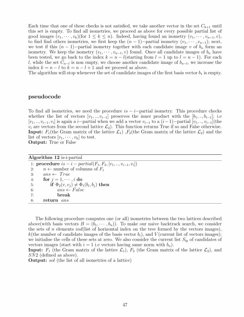
Each time that one of these checks is not satisfied, we take another vector in the set Ck+1 untilthis set is empty. To find all isometries, we proceed as above for every possible partial list ofgood images (v1, · · · , vk)(for 1 ≤ k ≤ n). Indeed, having found an isometry (v1, · · · , vn−1, v),to find find others isometries, we first keep the (n − 1)−partial isometry (v1, · · · , vn−1); next,we test if this (n − 1)−partial isometry together with each candidate image v of bn form anisometry. We keep the isometry (v1, · · · , vn−1, v) found. Once all candidate images of bn havebeen tested, we go back to the index k = n− l(starting from l = 1 up to l = n− 1). For eachl, while the set Cn−l is non empty, we choose another candidate image of bn−l, we increase theindex k = n− l to k = n− l + 1 and we proceed as above.The algorithm will stop whenever the set of candidate images of the first basis vector b1 is empty.

pseudocode

To find all isometries, we need the procedure is − i−partial isometry. This procedure checkswhether the list of vectors [v1, .., vi−1] preserves the inner product with the [b1, .., bi−1]; i.e[v1, .., vi−1, vi] is again a i−partial when we add a vector vi−1 to a (i−1)−partial [v1, .., vi−1](thevi are vectors from the second lattice L2). This function returns True if so and False otherwise.Input: F1(the Gram matrix of the lattice L1) ,F2(the Gram matrix of the lattice L2) and thelist of vectors [v1, · · · , vk] to test.Output: True or False

Algorithm 12 is-i-partial

1: procedure is− i− partial(F1, F2, [v1, .., vi−1, vi])2: n← number of columns of F1

3: ans← True4: for j = 1, · · · , i do5: if Φ2(v, vj) 6= Φ1(bi, bj) then6: ans← False7: break8: return ans

The following procedure computes one (or all) isometries between the two lattices describedabove(with basis vectors B = (b1, · · · , bn)). To make our naive backtrack search, we considerthe sets of n elements ind(list of horizontal index on the tree formed by the vectors images),k(the number of candidate images of the basis vector bi), and V (current list of vectors images);we initialise the cells of these sets at zero. We also consider the current list Stp of candidates ofvectors images (start with i = 1 i.e vectors having same norm with bn).Input: F1 (the Gram matrix of the lattice L1), F2 (the Gram matrix of the lattice L2), andSN2 (defined as above).Output: sol (the list of all isometries of a lattice)

47

Algorithm 13 All (or one) isometries of a lattice

1: procedure naive− algo− iso(F1, F2, SN2, one− iso = False)2: n ← number of columns of F1

3: Stp ← SN21, k1 ← len(Stp), i← 14: while i ≤ n and ind1 < k1 do5: ki ← len(Stp), f ind− vi ← False6: if i < n then7: for j = indi, · · · , ki do8: kpartial← [V1, · · · , Vi], appen(Stp[j], kpartial)9: L← cand− vect− iso(F1, F2, SN2, kpartial, i+ 1, i+ 1)

10: if is− i− partial(F1, F2, [v1, .., vi−1, vi]) then11: Vi ← Stp[j], Stp ← L, find− vi = True12: break13: else14: if j < ki − 1 then15: indi ← indi + 116: if find− vi then17: i← i+ 118: else19: while indi = ki − 1 and i > 1 do20: indi ← 0, i← i− 1

21: indi ← indi + 122: Stp← cand− vect− iso(F1, F2, SN2, [V1, · · · , Vi], i, i)23: else24: for j = 1, · · · , ki do25: if is− i− partial(F1, F2, [V1, .., Vn−1, Stp[j]]) then26: Vn ← Stp[j]27: append(V, sol)

28: if one− iso and length(sol) = 1 then29: return sol30: i← n− 131: while indi = ki − 1 and i > 1 do32: indi ← 0, i← i− 1



39: else40: Stp ← cand− vect− iso(F1, F2, SN2, [V1, · · · , Vi], i, i)41: return sol

48

This algorithm will terminates as the set Iso(L1,L2) is finite. Indeed, if g ∈ Iso(L1,L2)then g(bi) ∈ S2 for every 1 ≤ i ≤ n and the list (g(b1), · · · , g(bn)) determines g; This impliesthat |Iso(L1,L2)| ≤ |S2|n which is finite since the set of short vectors S2 (shown in chapter 3)is finite.

5.4 Isometries search with fingerprint

Here, we present an a method to compute either one or all isometries between the two latticesdescribed above using the fingerprint test. This fingerprint test is done using the fingerprint f1of the first lattice L1 (that is computed as in chapter 4) and the number of extensions in theisometry case.

Definition 50 The number of extensions (in the isometry case) of a k-partial isometry (v1, · · · , vk)is the number of vector v ∈ S2 satisfying:{

Φ2(v, v) = Φ1(bk+1, bk+1)

Φ2(v, vj) = Φ1(bk+1, bj), for j = 1, · · · , k.

This number is denoted by nbExt− iso. It is defined by:nbExt− iso(v1, · · · , vk) = |{v ∈ SN2k+1 : Φ2(v, vj) = Φ1(bk+1, bj), for j = 1, · · · , k}|.

For k-partial isometry (v1, · · · , vk), this number is simply zero as all vectors in the k-partialisometry are already good images of the basis vector b1 up to bk. Therefore, for any 1 ≤ i, k ≤ nand any k-partial isometry (v1, · · · , vk), we may consider the following:

nbExt− iso([v1, · · · , vk], k, i) =

{0 if i < k∣∣∣{v ∈ SN2i : Φ2(v, vj) = Φ1(bi, bj), for j = 1, · · · , k − 1}

∣∣∣ otherwise.

This number of extensions is exactly the number of candidate images Cki for each fixed i andk. To compute this number, we will use the following algorithm.

5.4.1 Algorithm to find the number of extensions

Here is an algorithm to find at a step k the list of candidates images Cki of a lattice elementwith same norm as the basis vector bi. We consider the lattices L1 and L2 as above.

Pseudocode

input: F1 (the Gram matrix of the lattice L1), F2 (the Gram matrix of the lattice L2) the setof same norm SN2, the k-partial isometry kpartial = [v1, · · · , vk] to test and the index k, i.output: nExt− iso (the number of extensions)

49

Algorithm 14 the list of candidates images Cki1: procedure nbExt− iso(F1, F2, SN2, kpartial, k, i)2: n← number of columns of F3: nExt− iso← length(cand− vect− iso(F1, F2, SN2, kpartial, k, i))4: return nExt− iso

To determine each such list of good image (v1, · · · , vn) of the basis vector using the fingerprinttest, the idea is to first consider the naive algorithm of the isometry described in the previoussection; Next, in that algorithm, before checking if the list (v1, · · · , vk, v) is a (k + 1)-partialautomorphism, we first check if the number of extensions of (v1, · · · , vk, v) corresponds to thenumber of extensions of (b1, · · · , bk, bk+1). This is helpful to detect as soon as possible, a k-partialisometry that cannot be extended into an isometry. The algorithm is the following.

Pseudocode

Input: F1 (the Gram matrix of the lattice L1), f1 (the fingerprint of the lattice L1), F2 (theGram matrix of the lattice L2), and SN2 (defined as above).Output: sol (the list of all isometries of a lattice)

50

Algorithm 15 All (or one) isometries of a lattice

1: procedure algo− iso− fingerprint(F1, f1, F2, SN2, one− iso = False)2: n ← number of columns of F1

3: Stp ← SN21, k1 ← len(Stp), i← 14: while i ≤ n and ind1 < k1 do5: ki ← len(Stp), f ind− vi ← False6: if i < n then7: for j = indi, · · · , ki do8: kpartial← [V1, · · · , Vi], append(Stp[j], kpartial)9: L← cand− vect− iso(F1, F2, SN2, kpartial, i+ 1, i+ 1)

10: if nbExt− iso(F1, F2, SN2, kpartial, i+ 1, + 1) = f1[i+ 1, i+ 1] then11: Vi ← Stp[j], Stp ← L, find− vi ← True12: break13: else14: if j < ki − 1 then15: indi ← indi + 116: if find− vi then17: i← i+ 118: else19: while indi = ki − 1 and i > 1 do20: indi ← 0, i← i− 1

21: indi ← indi + 122: Stp← cand− vect− iso(F1, F2, SN2, [V1, · · · , Vi], i, i)23: else24: for j = 1, · · · , ki do25: if is− i− partial(F1, F2, [V1, .., Vn−1, Stp[j]]) then26: Vn ← Stp[j]27: append(V, sol)

28: if one− iso and length(sol) = 1 then29: return sol30: i← n− 131: while indi = ki − 1 and i > 1 do32: indi ← 0, i← i− 1



39: else40: Stp ← cand− vect− iso(F1, F2, SN2, [V1, · · · , Vi], i, i)41: return sol

51

5.5 Search for Isometries of lattices

We follow the method describe in the above proposition. Recall that from the above proposition,to determine the set of all isometries between two lattices L1 and L2, the idea is to first determineonly one isometry g between these two lattices, then find all the automorphisms of the first latticeL1, and deduce Iso(L1,L2) by taking the composition of g with each of the automorphism foundof L. We will use the algorithm for isometry using fingerprint to determine the first isometry.And the algorithm of automorphisms described in chapter 3 to determine the automorphismsof the first lattice.

pseudocode

input: F1 (the Gram matrix of the lattice L1), f1 (the fingerprint of the lattice L1), SN1(defined as in the automorphism case), F2 (the Gram matrix of the lattice L2) and SN2 (definedas above).output: sol (the list of all isometries)

Algorithm 16 the list of candidates images Cki1: procedure algo− iso− auto(F1, f1, SN1, F2, SN2)2: sol = [ ]3: ”Computing the first isometry”4: g = algo− iso− fingerprint(F1, f1, F2, SN2, T rue)5: ”Computing the list of all automorphisms of the first lattice”6: List− auto1 = auto(F1, SN1, f1)7: for θ in List− auto1 do8: append(θ ◦ g, sol)9: return sol

5.6 Runtime of algorithms described

The aim of this section is to test and give the computation time of the three algorithms for findingisometries of lattices described above. This will be done on some examples where the bases ofthe lattices involved are isometrics or not. In the first section, we construct some isometricsbases to be used in order to ensure our algorithms results. The second section provided the testand the comparison of these algorithms on examples based on the construction of isometricsbases made.

5.6.1 Construction of isometrics lattices

In what follows, we would like to illustrate how one may construct two isometrics lattices. Itsuffices to construct from a given basis matrix B of the first lattice, a second basis matrix V

52

such that these two basis are isometrics. For this purpose, we consider two lattices with basisvectors: B = (b1, · · · , bn) and V = (v1, · · · , vn), and with bilinear forms given by the innerproduct. The following lemma is a tool for the construction of such basis.

Lemma 51 Assume that there exists coefficients αij ∈ Z such that bi =∑n

j=1 αijvj. Then thereexists an isometry g between B and V .

Proof. We set g(bi) =∑n

j=1 αijvj := bi, for each i = 1, · · · , n.

Since g(bi) := bi and the bilinear forms are given by the inner product, then g preserves thebilinear forms. It is a Z-linear bijection by definition. Moreover, from this definition, g sendseach coordinates (0, · · · , 0, 1, 0, · · · , 0)T (with 1 in the i-th position) of the basis vectors bi tothe coordinates vectors (αi1, αi2, · · · , αii, · · · , αin)T ; thus we get:

((b1, · · · , bn)) = (v1, · · · , vn)

α11 α21 · · · αn1...

... · · · ...α1n α2n · · · αnn

Hence, g is really an isometry that sends B to V .

From this lemma, we know that if we have basis vectors B and V as above such that thebi’s are linear combinations of the vi’s, then the basis B and V are isometrics. The followingproposition involve an example of construction of isometric basis.We consider B and V as above and we assume that:

v1 = b1v2 = α21b1 + b2

...

vk =k−1∑j=1

αkjbj + bk

...

vn =n−1∑j=1

αkjbj + bn

Proposition 52 Considering these assumptions, the basis B and V are isometrics.

Proof. From the above lemma, it suffices to show that there exists βij ∈ N such thatbi =

∑nj=1 βijvj for all i ∈ {1, · · · , n}.

We prove this by induction on i.

1) For i = 1: since v1 = b1, set β11 = 1 and β1j = 0 ∀j > 1 and get b1 =∑n

j=1 β1jvj.

53

2)Assume for i = 1, · · · , k that there exists βij ∈ N such that bi =∑n

j=1 βijvj. Let us prove

that there exists βk+1,j ∈ N such that bk+1 =∑n

j=1 βk+1,jvj.

We know that bk+1 = vk+1 −∑k

j=1 αk+1,jbj and by assumption ∀j ∈ {1, · · · , k} there exists

βjl ∈ N such that bj =∑n

l=1 βjlvl. From this, we get:

bk+1 = vk+1 −k∑j=1

αk+1,j

( n∑l=1

βjlvl

)= vk+1 −

n∑l=1

( k∑j=1

αk+1,jβjl

)vl

Since∑k

j=1 αk+1,jβjl ∈ N for all l, then one may set βk+1,l =∑k

j=1 αk+1,jβjl ∈ N. Thus

bk+1 =∑n

j=1 βk+1,jvj.This proves the proposition.

From this proposition, we can deduce the following corollary.

Corollary 53 Given a basis B = (b1, · · · , bn) and arbitrary coefficients αij ∈ N such thatαii = 1 for i = 1, · · · , n and αij = 0 for j > i and j ∈ {1, · · · , n}, one can construct anisometric basis V = (v1, · · · , vn) of B, with the vi’s defined by vi =

∑nj=1 αijbj = bi+

∑j<i αijbj.

Moreover, the basis V can be computed using the matrix expression: V = BM , where M =1 α21 · · · αn1

0 · · ...... · · αn,n−10 · 0 1

Proof. This is just a consequence of the above proposition.

5.6.2 Computation time

Here we use three examples to illustrate the test and to present the computation time of ouralgorithms.

Example 54 In this example, we want to verify whether our algorithms returns an empty listwhen they have as input not isometric lattices. For this purpose, we consider the identity latticen and the root lattice An with Gram matrix FAn defined with 2 on the diagonal entries, −1 under

54

and over the diagonal entries and the 0 elsewhere. It is given by:

FAn =

2 −1 0 · · · 0−1 · · · · · ·0 · · · ...... · · · 0· · · · −10 · · · 0 −1 2

.

These two lattices are not isometric as det(FIdn) = 1 6= 5 = det(FAn). We run our Sage codein dimension 4 and we get the following results.

Returns iso-naive iso-fingerprint iso-autotime(s) 0.0 0.0 0.0card(Iso(Id4,A4)) 0 0 0

This table ensure our algorithms results when not isometric lattices are given. Moreover, werealised that our Sage code produces this results in time less than a second.

The following example uses the above corollary to compute from a given basis B of a lattice,a second basis V for a second lattice in the case where M = (αij)(1≤i,j≤n), with n equals to thenumber of bi’s; the matrix M has 1 on the diagonal and under the diagonal, and the 0 in otherentries. Then, we find the isometries between B and V using our algorithms. The computationtime of these algorithms is also considered.

Example 55 Here, we take B =

(0 2 02 1 10 0 1

)and with our Sage code we compute V =

(2 2 03 2 10 1 1

).

Then we compute the Gram matrices FB = BTB and FV = V TV Finally, we apply these Grammatrices to our Sage code and we obtain the following results.

Returns iso-naive iso-fingerprint iso-autotime(s) 0.0 0.0 0.015card(Iso(B, V )) 16 16 16

55

Chapter 6

Conclusion

In this work, we first give an overview on lattices. This was done by giving definitions andexamples of lattice, lattice elements, quadratic and bilinear form associated to a given lattice;Also, we gave a brief description and application of some matrix decomposition; The definitionsand properties of automorphisms and isometries were also involved. Second, we describe amethod for computing short vectors of a given lattice (L,Φ); These are vectors v in L satisfyingΦ(v, v) ≤M , where M is the maximal norm of the basis vectors of the lattice L; These methodsuse either the Cholesky decomposition or the LDLT -decomposition of the LLL reduced form ofthe Gram matrix of the lattice involved; We also study the complexity analysis of these methodsbased on [4] and a computation time of these algorithms on an example. Third, we present analgorithm for computing the group of automorphisms of lattices; Proposed by [1], this methodis achieved using partial maps and the fingerprint of the Gram matrix involved; The descriptionof this backtrack search algorithm is followed by a computation time measurement. We end bypresenting methods to compute isometries between two lattices. These methods are based on thebacktrack search described on [1] to find the group of automorphisms of lattices. All algorithmsdescribed in this essay were coded and tested in Sage 8.1 using standard packages. Future workwith these methods would involve reducing the computation time by using for instance vectorsums or Bacher polynomials as in [1]. One can also use the algorithm for computing isometriesto construct the genus of lattices. Lastly, these methods could also be extended in general towork over number fields.

56

Acknowledgements

This essay owes its existence to the help, support and inspiration of kind people around me. Iwould like to extend my sincere thanks to all of them.

Above all, I am grateful to the almighty God for the divine intervention in this academicyear and for establishing me to complete this work.

I would like to express my deepest sense of gratitude to my supervisor Dr. Aurel Page. I amextremely grateful and indebted to him for his expertise, patience, sincere, valuable guidanceand encouragement extended to me. I place on record, my sincere thanks to my supervisorfor his unwavering support, understanding, corrections and encouragement. A special thank toPr. Dr Christine Bachoc for having allowed me to discover, to like, and to write my essay onArithmetic Number Theory.

I would like to offer my special appreciation and thanks to Pr.Dr. Marco Garuti, to Pr.Dr Bruno chiarellotto for their devotion and the ALGANT consortium for providing me all thenecessary facilities and for allowing me to spend a blessed and memorable academic years. Ispecially express my sincere thanks to Pr.Dr. Marco Garuti, for his constant encouragement,support and advices. A special thanks to all the lecturers who have greatly boosted my knowl-edge. I am very grateful.

I am thankful to all my family and friends. My lovely parents Annie Teagho and EtienneTeagho; my brothers and sisters, Frank, Yasmine, Urmes and Stan; my friends Chiara and MarieChristine, thank you to always believe in me and to always being there for me. A special thanksto my husband Walter Simo, for his unwavering support, corrections and encouragement. Youhave given me your unequivocal support throughout, as always, for which my mere expressionof thanks likewise does not suffice. A special thanks, to my course mates of the University ofBordeaux(France), you made my stay here at Bordeaux memorable. I end by placing on recordmy sense of gratitude to one and all who, directly or indirectly, have lent their helping hand inthis venture.

57

Bibliography

[1] W. PLESKEN and B. SOUVIGNIER. Computing isometries of lattices. Journal of SymbolicComputation, 24(3) :327-334, 1997.

[2] Christine Bachoc. Lecture Note, University of Bordeaux, 2017.

[3] Henri Cohen. A course in computational algebraic number theory, volume 138 of GraduateTexts in Mathematics. Springer-Verlag, Berlin, 1993.

[4] U. Fincke and M. Pohst. Improved methods for calculating vectors of short length in alattice, including a complexity analysis. Math. Comp., 44(170): 463-471, 1985.

[5] Guillaume Hanrot and Damien Stehle. Improved analysis of Kannans shortest lattice vectoralgorithm (extended abstract). In Advances in cryptology-CRYPTO 2007, volume 4622 ofLecture Notes in Comput. Sci., pages 170-186. Springer, Berlin, 2007.

[6] L. Lagrange. Recherches d’arithmetique. Nouv. Mdm. Acad, pages 265-312, 1773

[7] C.F. Gauss. Disquisitiones arithmeticae. 1801.

[8] Hermann Minkowski. Geometrie der Zahlen. Leipzig: Teubner, 1910.

[9] A. K. Lenstra, H. W. Lenstra, Jr., and L. Lovasz. Factoring polynomials with rationalcoefficients. 261(4):515-534, 1982

58

malonguemfo teagho amandine - u-bordeaux.fr

Documents