r emi boutonnet - u-bordeaux.fr

Lattices in semi-simple Lie groups

Remi Boutonnet

This course aims to present various constructions and properties of lattices in Lie groups.

I thank Yves Benoist for allowing me to use his lecture notes [Ben08]. Most of thetime, I did nothing more than translate his notes into english. Sometimes I added minordetails to proofs and I take full responsibility if mistakes or inconsistencies appear. Nooriginality is claimed.

Contents

Chapter 1. Locally compact groups and lattices 2

Chapter 2. Some facts on Lie groups 9

Chapter 3. Ergodic theory and unitary representations 18

Chapter 4. Projective dynamics 31

Chapter 5. Extra topics 38

Chapter 6. Margulis superrigidity theorem 44

Bibliography 54

1

CHAPTER 1

Locally compact groups and lattices

1. The Haar measure

Definition 1.1. A topological group is a group G endowed with a topology for which themap (g, h) ∈ G×G→ gh−1 is continuous. G is said to be locally compact if every pointadmits a compact neighborhood, or equivalently if the trivial element admits a compactneighborhood.

In the above terminology, the term compact includes the Hausdorff axiom, according tothe French convention.

Example 1.2. We will encounter many locally compact groups.

• All Lie groups are examples of locally compact groups.• Any group can be made locally compact by considering its discrete topology.

This is the topology we will usually use for countable groups.• The additive group (Qp,+) is locally compact (for the topology given by its

ultrametric norm), and the subgroup Zp ⊂ Qp is a compact neighborhood of 0.

Definition 1.3. A Haar measure on a locally compact group is a (non-zero) Radonmeasure λ on G which is invariant under left translation, in the sense that for all g ∈ G,and all Borel set A ⊂ G, λ(gA) = λ(A).

We recall that a Radon measure is a Borel measure which is finite on compact sets andregular, meaning that for any Borel set A,

λ(A) = supλ(K) | K ⊂ A compact = infλ(U) | U open set containing A.

Example 1.4. If G = (R,+), the Lebesgue measure is a Haar measure. The countingmeasure on a discrete group is a Haar measure.

The following observation follows from standard considerations on measurable functions.

Lemma 1.5. A Radon measure λ on a locally compact group is a Haar measure if andonly if for every f ∈ Cc(G) and every g ∈ G, we have

∫Gf(x)dλ(x) =

∫Gf(gx)dλ(x).

Theorem 1.6. If G is a locally compact group it always admits a Haar measure. More-over, any two Haar measures on G are proportional.

We will not prove the existence part in this theorem because, one, it is rather long todo and not much more instructive than the usual construction of the Lebesgue measure,and two, because for our examples a Haar measure can often be found by more concretemethods. For example, one can easily construct a left invariant volume form on a Liegroup: just pick an n-form on the tangent space at the identity of the Lie group G (wheren = dim(G)) and propagate it using the left translations Lg, g ∈ G. We shall see how toconcretely compute a Haar measure for G = SL2(R). Moreover, for all discrete groupswe already explained that the counting measure is a Haar measure.

2

1. THE HAAR MEASURE 3

Proof. Let us prove the proportionality statement. Fix a Haar measure λ.

Claim 1. For all non-zero function f ∈ Cc(G) such that f ≥ 0 we have∫Gfdλ 6= 0.

To prove this claim, note that given such a function f , there exists ε > 0 such thatU := x ∈ G | f(x) ≥ ε is non-empty, and of course we have f ≥ ε1U . So it suffices toprove that λ(U) > 0 for any non-empty open set U in G. By assumption, λ is non-zeroso there exists a Borel set A such that λ(A) 6= 0. Since λ is moreover regular we mayactually find a compact subset K ⊂ A such that λ(K) 6= 0.

If U ⊂ G is a non-empty open set, the collection of translates gU , g ∈ G is an open coverof G, and in particular, of K. By compactness of K, we may extract from it a finitesub-cover. In other words we find a finite set F ⊂ G such that K ⊂ ∪g∈FgU . But thisleads to an inequality on measures:

0 < λ(K) ≤∑g∈F

λ(gU) = |F |λ(U).

So we indeed arrive at the conclusion that λ(U) 6= 0, and Claim 1 follows.

Fix two non-zero functions f, g ∈ Cc(G), such that f, g ≥ 0. For notational simplicity,we denote by λ(f) :=

∫Xf dλ and λ(g) =

∫Xg dλ.

Claim 2. The ratio λ(f)/λ(g) makes sense thanks to Claim 1. It does not depend on λ.

Assume that µ is another Haar measure on G. We consider the function h : G×G→ Rgiven by the formula

h(x, y) = f(x)a(x)g(yx), where a(x) = (

∫G

g(tx) dµ(t))−1.

This is easily seen to be a compactly supported continuous function. Moreover, our choiceof normalization by a(x) gives

∫Gh(x, y)dµ(y) = f(x) for all x ∈ G. Therefore,∫

G

∫G

h(x, y) dµ(y) dλ(x) = λ(f).

On the other hand, since h is compactly supported and continuous, it is integrable, andFubini theorem applies. Combining it with the fact that λ and µ are left invariant we get∫

G×Gh(x, y) dµ(y) dλ(x) =

∫G×G

f(x)a(x)g(yx) dλ(x) dµ(y)

=

∫G×G

f(y−1x)a(y−1x)g(x) dλ(x) dµ(y)

=

∫G×G

f(y−1)a(y−1)g(x) dµ(y) dλ(x).

So we arrive at

λ(f) =

∫G

g(x) dλ(x)

∫G

f(y−1)a(y−1) dµ(y) = Cλ(g),

where C =∫Gf(y−1)a(y−1) dµ(y), which does not depend on λ. This proves Claim 2.

Now if λ′ is another Haar measure, we get for any two non-negative, non-zero functionsf, g ∈ Cc(G),

λ(f) =λ(g)

λ′(g)λ′(f).

1. THE HAAR MEASURE 4

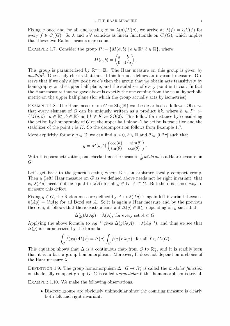
Fixing g once and for all and setting α := λ(g)/λ′(g), we arrive at λ(f) = αλ′(f) forevery f ∈ Cc(G). So λ and αλ′ coincide as linear functionals on Cc(G), which impliesthat these two Radon measures are equal.

Example 1.7. Consider the group P := M(a, b) | a ∈ R∗, b ∈ R, where

M(a, b) =

(a b0 1/a

).

This group is parametrized by R∗ × R. The Haar measure on this group is given byda db/a2. One easily checks that indeed this formula defines an invariant measure. Ob-serve that if we only allow positive a’s then the group that we obtain acts transitively byhomography on the upper half plane, and the stabilizer of every point is trivial. In factthe Haar measure that we gave above is exactly the one coming from the usual hyperbolicmetric on the upper half plane (for which the group actually acts by isometries).

Example 1.8. The Haar measure on G := SL2(R) can be described as follows. Observethat every element of G can be uniquely written as a product hk, where h ∈ P 0 :=M(a, b) | a ∈ R∗+, b ∈ R and k ∈ K := SO(2). This follow for instance by consideringthe action by homography of G on the upper half plane. The action is transitive and thestabilizer of the point i is K. So the decomposition follows from Example 1.7.

More explicitly, for any g ∈ G, we can find a > 0, b ∈ R and θ ∈ [0, 2π[ such that

g = M(a, b)

(cos(θ) − sin(θ)sin(θ) cos(θ)

).

With this parametrization, one checks that the measure 1a2dθ da db is a Haar measure on

G.

Let’s get back to the general setting where G is an arbitrary locally compact group.Then a (left) Haar measure on G as we defined above needs not be right invariant, thatis, λ(Ag) needs not be equal to λ(A) for all g ∈ G, A ⊂ G. But there is a nice way tomeasure this defect.

Fixing g ∈ G, the Radon measure defined by A 7→ λ(Ag) is again left invariant, becauseh(Ag) = (hA)g for all Borel set A. So it is again a Haar measure and by the previoustheorem, it follows that there exists a constant ∆(g) ∈ R∗+, depending on g such that

∆(g)λ(Ag) = λ(A), for every set A ⊂ G.

Applying the above formula to Ag−1 gives ∆(g)λ(A) = λ(Ag−1), and thus we see that∆(g) is characterized by the formula∫

G

f(xg) dλ(x) = ∆(g)

∫G

f(x) dλ(x), for all f ∈ Cc(G).

This equation shows that ∆ is a continuous map from G to R∗+, and it is readily seenthat it is in fact a group homomorphism. Moreover, It does not depend on a choice ofthe Haar measure λ.

Definition 1.9. The group homomorphism ∆ : G→ R∗+ is called the modular functionon the locally compact group G. G is called unimodular if this homomorphism is trivial.

Example 1.10. We make the following observations.

• Discrete groups are obviously unimodular since the counting measure is clearlyboth left and right invariant.

2. LATTICES IN LOCALLY COMPACT GROUPS 5

• Compact groups are unimodular. To see this observe that any Haar measure λon such a group G is finite. Thus we have ∆(g)λ(G) = λ(Gg−1) = λ(G) for allg ∈ G, showing that ∆ has constant value 1.• Since the modular function is a character G → R∗+, any group that does not

admit a character is unimodular. For instance simple groups are unimodular.This also gives another proof that compact groups are unimodular.

Remark 1.11. One should be careful that unimodularity doesn’t pass to subgroups. Inparticular, the restriction of the modular function ∆G of a group G to a subgroup Hneeds not be the modular function ∆H of the subgroup.

For example, we deduce from the previous exemple that SL2(R) is unimodular, since it hasno character. On the other hand it contains the subgroup H := M(a, b) | a ∈ R∗, b ∈ R,where

M(a, b) =

(a b0 1/a

).

But one verifies that the modular function on H is given by ∆H(M(a, b)) = a2, which isnon-trivial.

2. Lattices in locally compact groups

Definition 1.12. If G is a topological group, a discrete subgroup Γ < G is a subgroupwhich is discrete in G for the induced topology. This amounts to saying that there is aneighborhood U ⊂ G of the trivial element e ∈ G such that U ∩ Γ = e.

We will restrict our attention to locally compact, second countable groups (i.e. thoseadmitting a countable basis of open sets). We write lcsc for short.

Lemma 1.13. For any discrete group Γ in a lcsc group there always exists a Borel fon-damental domain, i.e. a Borel subset F ⊂ G such that FΓ = G and Fg ∩Fh = ∅ for alldistinct elements g, h ∈ Γ.

Proof. Fix a neighborhood V ⊂ G of e such that V ∩Γ = e, and pick a neighbor-hood U ⊂ G of e such that U−1U ⊂ V . This is possible because the map (g, h) 7→ g−1his continuous on G × G. Since G is second countable, there exists a countable set ofelements (gn)n≥1 in G such that G =

⋃n≥1 gnU .

Define inductively a sequence of Borel sets Fn ⊂ G, n ≥ 1 as follows. Set F1 = g1U and

Fn+1 = gn+1U \

(gn+1U ∩

n⋃k=1

gkUΓ

).

These are disjoint sets and better, for every n 6= m we have FnΓ ∩ FmΓ = ∅, whilen⋃k=1

FkΓ =n⋃k=1

gkUΓ.

So the set F =⋃nFn is a Borel set such that FΓ = G. Assume now that g, h ∈ Γ are two

elements such that Fg ∩ Fh 6= ∅. There exist two indices such that Fng ∩ Fmh 6= ∅. Byconstruction this forces n and m to be equal. Since Fn ⊂ gnU we can then find x, y ∈ Usuch that gnxg = gnyh, which leads to x−1y = gh−1 ∈ V ∩ Γ = e. So we conclude thatg = h.

Thus F is indeed a Borel fundamental domain.

2. LATTICES IN LOCALLY COMPACT GROUPS 6

Definition 1.14. A discrete subgroup Γ in a locally compact group G is called a latticeif it admits a Borel fundamental domain with finite Haar measure.

Example 1.15. It is trivial to see that Zn is a lattice in Rn, for which a fundamentaldomain is given by [−1, 1[n.A less trivial example is that of SL2(Z) inside SL2(R). To see that this is indeed a lattice,one can use the fact that the action of SL2(Z) on the hyperbolic half-plane admits aBorel fundamental domain with finite measure. We leave the details as an exercise. Inthe same spirit, the fundamental group of any compact surface with negative curvatureembeds as a lattice inside PSL2(R).

Lemma 1.16. Let Γ be a discrete subgroup in a lcsc group G. Then any two Borelfondamental domains for Γ have the same right-Haar measure.

Proof. Let F and F ′ be two fundamental domains and denote by λ a right-Haarmeasure on G. Then we have

λ(F) =∑g∈Γ

λ(F ∩ F ′g) =∑g∈Γ

λ(Fg−1 ∩ F ′) = λ(F ′).

We used implicitly the fact that Γ is countable, which is automatic if it is discrete andG is lcsc.

Corollary 1.17. If G is a lcsc group admitting a lattice Γ then it is unimodular. More-over, there exists a G-invariant Borel probability measure on G/Γ.

Proof. Let λ be a right Haar measure on G, and denote by F a fundamental domainfor Γ. Then for every g ∈ G, gF is also a fundamental domain for Γ. So λ(F) = λ(gF),hence λ is left invariant, which implies that G is unimodular.

Moreover, let us restrict the projection map p : G → G/Γ to the Borel subset F . Thenthe restriction of λ to F is a finite measure (and we may normalize it so that it is aprobability measure). Its push forward on G/Γ is also a finite measure νF which dependsa priori on F . Let us check that this is not the case. Take another fundamental domainF ′. Take A ⊂ G/Γ, and denote by B := p−1(A). We have

νF(A) = λ(B ∩ F) =∑g∈Γ

λ(B ∩ F ∩ F ′g).

In the last inequality above, we used the fact that G is the disjoint union of the setsFg, g ∈ Γ. Now since the measure λ is right-invariant and since B is globally rightΓ-invariant, we further find

νF(A) =∑g∈Γ

λ(B ∩ Fg−1 ∩ F ′) = λ(B ∩ F ′) = νF ′(A).

Now observe that for g ∈ G, the left translation by g maps the fundamental domain Fto F ′ = gF , and since it preserves the Haar measure λ, we find that g∗νF = νgF . SinceνF does not depend on F , we get that it is g-invariant.

Proposition 1.18. Let G be a unimodular lcsc group and take a discrete subgroup Γ inG. The following facts are equivalent.

(i) Γ is a lattice in G;(ii) There exists a Borel set Ω ⊂ G with finite right Haar measure such that ΩΓ = G;

(iii) There exists a G-invariant Borel probability measure on G/Γ.

3. SOME EXTRA EXAMPLES 7

Proof. The implication (i) ⇒ (ii) is tautologic and its converse is proved similarlyto Lemma 1.13 (one just needs to intersect all the sets with Ω all along the proof of thatlemma). The previous corollary showed (i) ⇒ (iii). Let us prove the converse. This iswhere we will use the unimodularity assumption.

Denote by ν ∈ Prob(G/Γ) a G-invariant probability measure. The choice of a Borelfundamental domain F for Γ gives rise to an isomorphism of measure spaces

G/Γ× Γ ' F × Γ ' G.

We only need to check that the measure ν × c, where c is the counting measure on Γ,is transported to a left invariant measure on G. Once we do this, we will conclude thatthe fundamental domain F ⊂ G has finite left Haar measure, and hence finite right Haarmeasure by unimodularity.

Exercise. Prove that the above isomorphism transports the left action of G on itself tothe action of G on G/Γ × Γ given by the formula g(x, γ) = (gx, c(g, x)γ), for all g ∈ G,x ∈ G/Γ, γ ∈ Γ, where c(g, x) is the element such that gh ∈ Fc(g, x), where h ∈ F is therepresentative of x ∈ F . Prove that the measure ν × c is invariant under this action.

3. Some extra examples

A sufficient condition to be a lattice is to be co-compact.

Definition 1.19. A closed subgroup H in a lcsc group G is said to be co-compact if thequotient G/H is compact for the quotient topology.

Lemma 1.20. If Γ is a co-compact discrete subgroup of G, then it is a lattice.

Proof. As we already mentioned, the quotient map p : G→ G/Γ is open. Let U bea non-empty open set in G with compact closure. Then we may cover G by left translatesof U . Then the family p(gU), g ∈ G is an open cover of G/Γ. So if Γ is co-compact in G,we may find a finite set F ⊂ Γ such that G/Γ =

⋃g∈F p(gU). The subset Ω :=

⋃g∈F gU

has compact closure (so it must have finite measure) and satisfies ΩΓ = G. We concludethat Γ is a lattice in G.

In the exercise sheets it is explained how to prove that SLn(Z) is a lattice in SLn(R).

Example 1.21. Γ = SLn(Z) is not co-compact in G = SLn(R). Here is why.

• The unipotent element γ = id +E1,2 ∈ Γ and the sequence of diagonal matricesgn = diag(1/n, n, 1, . . . , 1) ∈ G satisfy limn gnγg

−1n = id (also denoted by e).

• Assume by contradiction that G/Γ is compact, and thus, that some subsequencegnk

Γ converges to an element hΓ ∈ G/Γ. Then we may write gnk= hkγk with

hk ∈ G, γk ∈ Γ and limk hk = h ∈ G.• Then γkγγ

−1k = h−1

k (gnkγg−1

nk)hk converges to h−1eh = e. But this is a sequence

of elements in Γ. Since Γ is discrete in G, this forces γkγγ−1k = e for k large

enough, and hence γ = e. This is absurd.

Nevertheless, any simple Lie group, such as SLn(R), has plenty of co-compact and nonco-compact lattices. The main construction is of arithmetic nature. More precisely, Boreland Harish-Chandra proved that if G is an algebraic group defined over Q, that admitsno Q-character, then its set of integer points G(Z) is a lattice in its set of real points(which is a Lie group). We will not give details, but some of the definitions will be givenin the chapter on superrigidity.

3. SOME EXTRA EXAMPLES 8

Moreover, a criterion of Godement says exactly when G(Z) is co-compact in G(R): it isexactly when G(Z) does not have unipotent element. One direction is easy and followsessentially the argument that we used to show that SLn(Z) is not co-compact.

Example 1.22. We admit the following examples.

(1) Denote by q : Rn → R a non-degenerate quadratic form with rational entries.Then SO(q,Z) is a lattice in SO(q,R).

(2) Z[√

2] embeds into R in two ways. This gives two embeddings of SLn(Z[√

2]) inSLn(R). Then the diagonal embedding SLn(Z[

√2]) ⊂ SLn(R) × SLn(R) gives a

lattice. This case follows from restriction of scalars.(3) The theorem of Borel and Harish Chandra also generalizes to the more general

framework of S-adic algebraic integers. This allows to say that the diagonalembedding of SLn(Z[1/p]) into SLn(R)× SLn(Qp) is a lattice.

Note that if Γ1 < G1 and Γ2 < G2 are lattices, then Γ1 × Γ2 < G1 ×G2 is also a lattice.This case is called reducible.

Definition 1.23. A lattice Γ in a product of groups∏n

i=1Gi is said to be irreducibleif its projection on a sub-product

∏i∈J Gi has dense image as soon as J ( 1, n is a

proper subset.

For example, the examples (2) and (3) given above are irreducible.

CHAPTER 2

Some facts on Lie groups

1. Basic definitions and examples

1.1. Lie groups.

Definition 2.1. A Lie group is a smooth manifold G over R which admits a groupstructure such that the corresponding structure map m : (x, y) ∈ G × G 7→ xy−1 ∈ Gis smooth. A morphism between two Lie groups will be by definition a smooth grouphomomorphism.

We will only focus on real Lie groups. But many results from these notes also hold foranalytic Lie groups over Qp.

Among the first obvious examples we can think of, the groups Rn and its quotient Tn =Rn/Zn are Lie groups. More interestingly, the multiplicative group GLn(R) is an openset inside Mn(k). As such, it may be endowed with the corresponding smooth structure.It is of dimension n2 as a manifold. The other examples we will describe are actuallyrealized as closed subgroups of GLn(R).

Example 2.2. It is a theorem of Cartan and von Neumann that a closed subgroup Hof a Lie group G is a Lie group (and naturally, the manifold structure on H is so thatthe inclusion H ⊂ G is a smooth embedding). So all the following classical examples areclearly Lie groups (but this can also be checked using the submersion theorem).

• The Heisenberg group is the subgroup of GL3(R) consisting of upper triangularmatrices with 1’s on the diagonal. It is a nilpotent Lie group. The larger groupof all upper triangular matrices is also a Lie group, and it is solvable.• The special linear group SLn(R), consisting of matrices with determinant 1.• The orthogonal group O(p, q), associated to a non-degenerate quadratic form

of signature (p, q). We will denote by SO(p, q) the intersection of O(p, q) withSLn(R), and we use the notation O(n) = O(n, 0) and SO(n) = SO(n, 0).• The isometry group SO(n,R) n Rn is a Lie group (endowed with the product

structure as a manifold). It is the Lie group of orientation preserving isometriesof Rn. It can be realized as a subgroup of SLn+1(R):

SO(n,R) nRn '(

A u0 1

) ∣∣∣∣A ∈ SO(n,R), u ∈ Rn

.

More generally we can define unitary and symplectic analogues to orthogonal groups.

1.2. The Lie algebra of a Lie group. The advantage with Lie groups is that theycome with a so-called Lie algebra, giving all the tools from linear algebra to study them.

Definition 2.3. A Lie algebra is a finite dimensional vector space V , endowed with abilinear map [·, ·] : V ×V → V (the so-called Lie bracket) which satisfies the two axioms:

• [X, Y ] = −[Y,X] for all X, Y ∈ V (anti-symmetry);

9

1. BASIC DEFINITIONS AND EXAMPLES 10

• [X, [Y, Z]] + [Y, [Z,X]] + [Z, [X, Y ]] = 0 for all X, Y, Z ∈ V (Jacobi identity).

In order to define the Lie algebra of a Lie group G we introduce some terminology.Recall that a vector field on the manifold G is a derivation of the algebra C∞(G), thatis, a linear map X : C∞(G) → C∞(G) such that X(f1f2) = f1X(f2) + f2X(f1), for allf1, f2 ∈ C∞(G). Besides, for any g ∈ G, the translation map Lg : h ∈ G 7→ gh ∈ Ginduces a map τg : f 7→ f Lg on C∞(G). A vector field X on G is called left-invariantif it commutes with τg for all g ∈ G, i.e. X(f Lg) = (X(f)) Lg, for all f ∈ C∞(G).Note that this formula is equivalent to

(X(f))(g) = (X(f Lg))(e) for all g ∈ G.We write Xg(f) instead of X(f)(g). We denote by L(G) the vector space of all left-invariant derivations of C∞(G). Then the map X ∈ L(G) 7→ Xe ∈ Te(G) is a linearisomorphism from L(G) into the tangent space to G at e. In particular L(G) is finitedimensional.

Exercise 2.4. Given two left invariant vector fields X, Y on C∞(G), we may define theircomposition XY : C∞(G) → C∞(G). While this map still commutes with τg, g ∈ G, itis no longer a derivation in general.

• However, check that [X, Y ] := XY − Y X is again a left invariant derivation.• Check that (L(G), [·, ·]) is a Lie algebra.

Definition 2.5. The Lie algebra of left invariant derivations on C∞(G) with the abovebracket is called the Lie algebra of G. It is denoted by g.

Example 2.6. The Lie algebra of G = GLn(k) is Mn(k), endowed with the Lie bracket

[X, Y ] = XY − Y X.Let us indicate how to prove this fact. First observe that since GLn(k) is open in-side Mn(k), the tangent space at every point is naturally identified with Mn(k). Nowgiven a vector X ∈ Mn(k), we view it as a left-invariant vector field by the formulag ∈ G 7→ gX ∈ Mn(k) ' TgG. Its effect on C∞(G) is given by X(f)(g) = (df)g(gX)for all f ∈ C∞(G), g ∈ G. Differentiating further, we see that for all X, Y ∈ Mn(k),Y (X(f))(g) = (d2f)g(gX, gY )+(df)g(gY X). Since the second derivative d2(f)g is a sym-metric bilinear form, we get (Y (X(f))(g)−X(Y )(f))(g) = (df)g(gXY )− (df)g(gY X) =(XY − Y X)(f)(g), as desired.

Now recall that for any sub-manifold N ⊂ M defined by a submersion φ : M → M ′

as N = φ−1(x), the tangent space of N at a point is just the kernel of the derivativeof φ at that point. In particular we may compute the Lie algebras of all the standardexamples mentioned above.

Example 2.7. We have the following computations. We only describe the underlyingvector space, because the Lie bracket is simply the restriction of the Lie bracket on Mn(k).

• The Lie algebra of the Heisenberg group consists of all upper triangular matrices,with 0’s one the diagonal.• Since the derivative of the determinant map is the trace, the Lie algebra of SLn(k)

is the vector space of trace 0 matrices in Mn(k);• The Lie algebra ofO(n) is the subspace of matricesX such thatXT+X = 0 (anti-

symmetric matrices). More generally the Lie algebra of O(p, q) is the subspaceof matrices such that Ip,qX

T Ip,q + X = 0, where Ip,q is the diagonal matrixIp,q = diag(1, . . . , 1,−1, . . . ,−1), where 1 appears p times and −1 appears qtimes.


1.3. Functoriality. The following lemma asserts that taking the Lie algebra of aLie group is a functor.

Lemma 2.8. Consider two Lie groups G and H, with respective Lie algebras g and h. Ifφ : G → H is a differentiable homomorphism then its derivative dφ : g → h is a Liealgebra homomorphism.

Proof. Here we need to define properly the derivative dφ. Note that φ defines bypre-composition an algebra homomorphism φ∗ : f ∈ C∞(H) 7→ f φ ∈ C∞(G). Thenif X ∈ g is a left invariant derivation, X(f φ) is again in C∞(G) and we would like tocheck that it is of the form X ′(f) φ, and ensure that the map X ′ : C∞(H) → C∞(H)makes the following diagram commute.

C∞(H) C∞(G)

C∞(H) C∞(G)

φ∗

X′ X

φ∗

For every f ∈ C∞(H) and g ∈ G, we have X(f φ)(g) = X(f φ Lg)(e). Moreover,since φ is a group homomorphism, we have φ Lg = Lφ(g) φ. So,

(1.1) X(f φ)(g) = X(f Lφ(g) φ)(e) = X ′(f)(φ(g)),

where X ′ is the derivation on H defined by the formula X ′(f) : h ∈ H 7→ X(f Lhφ)(e).It is checked to be a left invariant derivation. Then we see that dφ : X 7→ X ′ is a linearmap between the Lie algebras g and h making the above diagram commute.

We now check that this is in fact a Lie algebra homomorphism. Take X, Y ∈ g. Denoteby X ′ := dφ(X) and Y ′ := dφ(Y ). For all f ∈ C∞(H) and g ∈ G, equation (1.1) gives

X ′(Y ′(f))(φ(g)) = X(Y ′(f) φ)(g) = X(Y (f φ))(g).

This immediately gives the computation

(X ′Y ′ − Y ′X ′)(f)(φ(g)) = (XY − Y X)(f φ)(g) = [(dφ)(XY − Y X)](f)(φ(g)).

So the vector fields X ′Y ′−Y ′X ′ and (dφ)(XY −Y X) coincide on φ(G) and in particularat e. Since they are both left invariant, they must coincide, which proves that dφ is a Liealgebra homomorphism.

In the above proof, observe that the definition of dφ that we gave coincides with theclassical differential (dφ)e : TeG → TeH when we identify the Lie algebras g and h withTeG and TeH as vector spaces. Using the structure theorems for sub-immersions one canprove the following property.

Proposition 2.9. Consider two Lie groups G and H and a Lie group homomorphismφ : G→ H. Then

(1) The kernel of φ is a closed Lie subgroup of G. Its Lie algebra is the kernel of dφ;(2) The image of φ is a (not necessarily closed) Lie subgroup of H; its Lie algebra

is the image of dφ;(3) If K ⊂ H is a closed subgroup of H with Lie algebra k, then φ−1(K) is a closed

subgroup of G whose Lie algebra is (dφ)−1(k).

Example 2.10. Pick a point in a ∈ R2 which is not a multiple of a point in Q2 e.g.a = (1,

√2). Then the image of the homomorphism t ∈ R 7→ ta ∈ T2 = R2/Z2 is a Lie

subgroup which is dense in T2 (hence not closed).


Item (3) above implies the following fact.

Corollary 2.11. If π : G→ GL(V ) is a smooth representation of a connected Lie groupG on a finite dimensional vector space V , then a subspace W ⊂ V is globally invariantunder π(G) if and only if it is invariant under (dπ)(g).

Proof. The computation of Example 2.6 gives that H = GL(V ) is a Lie group withLie algebra h = End(V ). The subgroup K := g ∈ GL(V ) | g(W ) = W is a closedsubgroup with Lie algebra k = X ∈ End(V ) | X(W ) ⊂ W.If W is π(G) invariant, then π−1(K) = G and Proposition 2.9.(3) implies that (dπ)−1(k) =g, which means exactly that W is invariant under dπ(g). Conversely, if W is invariantunder dπ(g), then Proposition 2.9.(3) implies that π−1(K) has Lie algebra g. So thesubgroup π1(K) of G has the same dimension as G. This implies that it is open in G,hence it is also closed in G, and by connectedness, it is equal to G. This means that Wis G invariant.

1.4. How much the Lie algebra remembers. We want to know to what extendgroups with the same Lie algebra are the same. Obviously, a Lie group and its identityconnected component have the same Lie algebra, because the latter is open inside theformer and the Lie algebra is a local data. But even in the connected setting, there existdifferent Lie groups with the same Lie algebra. For instance this is the case of R andR/Z. In the same spirit SL2(R) and PSL2(R) have the same Lie algebra.

Lemma 2.12. The universal cover G of a connected Lie group G is naturally endowed with

a Lie group structure such that the covering map G→ G is a Lie group homomorphism.

Its kernel is contained in the center of G.

Proof. Denote by π : G→ G the covering map. Fix a lift e of the identity element

eG. We define the product on G as follows. For g, h ∈ G, choose paths t 7→ gt, ht ∈ Gbetween e and g, h: g0 = h0 = e, g1 = g, h1 = h. The product path t 7→ π(gt)π(ht) in

G is a path between eG and π(g)π(h). Lift it to a path γ inside G starting at e. We setgh := γ(1). One checks that this definition is independent of the choices of paths thatwe made.

It is then easy to verify that this product law is associative, that e is a neutral element,and that the inverse g−1 of g is the end point of a lift starting at e of the path t 7→ π(gt)

−1.Moreover the covering map π is clearly a group homomorphism. Since it is also a local

homeomorphism, we may define the analytic structure of G by declaring that π is locallyanalytic. The fact that G is a Lie group implies that the structure map (g, h) 7→ gh−1 isanalytic.

Finally, take g, h ∈ G, with π(g) = e. Take a path t 7→ gt from e to g such that gt = gfor all t ≥ 1/2 and a path t 7→ ht from e to h such that ht = e for all e ≤ 1/2. We have:

• π(gt)π(ht) = π(gt) = π(ht)π(gt) if t ≤ 1/2;• π(gt)π(ht) = π(g)π(ht) = π(ht) = π(ht)π(gt) if t ≥ 1/2.

So gh = hg, as desired.

A connected Lie group is always locally isomorphic to its universal cover in the followingsense.


Definition 2.13. Two Lie groups G and H are said to be locally isomorphic if thereexist open neighborhoods U ⊂ G and V ⊂ H of the identity elements eG and eH and ananalytic diffeomorphism ϕ from U onto V such that ϕ(gh) = ϕ(g)ϕ(h) for all g, h ∈ Usuch that gh ∈ U .

Theorem 2.14. Consider two Lie groups G and H with Lie algebras g and h. Denote by

G and H the universal covers of the identity components of G and H respectively. Thefollowing are equivalent.

(i) G and H are locally isomorphic;

(ii) G and H are isomorphic;(iii) g and h are isomorphic.

Proof. To prove that (i) ⇔ (ii) first observe that being locally isomorphic is an

equivalence relation and that G (resp. H) is locally isomorphic with G (resp. H). Thenstandard topological considerations show that two simply connected groups are locallyisomorphic if and only if they are isomorphic.

The implication (ii) ⇒ (iii) follows from Lemma 2.8. The hard part is the converse,which we admit.

In particular if two simply connected Lie groups have the same Lie algebra, they mustbe isomorphic. There is also another situation where we can avoid the covering noise.

Corollary 2.15. If G,H are connected groups with trivial center and isomorphic Liealgebras, then they are isomorphic.

Proof. Theorem 2.14 implies that G and H have isomorphic universal cover : G 'H. But recall that the covering map p : G→ G is a group homomorphism whose kernel

is contained in the center of G. Since G has trivial center, we conclude that the kernel of

p is exactly the center of G (which thus must be discrete in G). Therefore G ' G/Z(G).

Likewise H ' H/Z(H), which implies that G ' H.

1.5. The adjoint representation. There are in fact two adjoint representations.

Lie group setting. Given a Lie group G, we may define for each g ∈ G a smooth au-tomorphism I(g) : h ∈ G 7→ ghg−1 ∈ G. Such group automorphisms are called innerautomorphisms. The differential of I(g) at e is then an invertible endomorphism of theLie algebra g of G, denoted by Ad(g) ∈ L(g); it is even a Lie algebra automorphism.The mapping Ad : G → GL(g) is then a linear representation of G, called the adjointrepresentation.

Lie algebra setting. A derivation of a Lie algebra g is a linear map D : g → g such thatD([X, Y ]) = [DX, Y ] + [X,DY ] for all X, Y ∈ g. One checks that if D and D′ are twoderivations, then so is DD′ − D′D. This operation turns the vector space Der(g) of allderivations of g into a Lie algebra.

It follows from the Jacobi identity that for any X ∈ g, the endomorphism ad(X) : g→ gis actually a derivation, called an inner derivation. The map ad : g→ Der(g) is actuallya Lie algebra homomorphism, called the adjoint representation. The term representationof a Lie algebra refers to a Lie algebra homomorphism from a given Lie algebra into theLie algebra L(V ) of all endomorphisms of a finite dimensional vector space V , endowedwith the Lie bracket of [X, Y ] = XY − Y X. Since ad is a representation, its image is aLie subalgebra of Der(g).

2. SEMI-SIMPLE LIE GROUPS 14

Lemma 2.16. Take a Lie group G with Lie algebra g. The group Aut(g) of all auto-morphisms of g is a Lie group. Its Lie algebra is Der(g). The derivative of the adjointrepresentation Ad : G→ Aut(g) of G is the adjoint representation ad : g→ Der(g) of g.

We admit this fact. It is based on properties of the exponential mapping.

Lemma 2.17. The kernel of the adjoint representation of a connected Lie group is itscenter.

Proof. Observe that the differential of the map p : (g, h) 7→ gh−1 at the point (e, e)is given by dp(e,e,)(X, Y ) = X − Y , for all X, Y ∈ g. By the chain rule, this implies thatfor a fixed g ∈ G, the derivative of the map f : h 7→ ghg−1h−1 = p(I(g)(h), h) at e isgiven by X 7→ Ad(g)(X)−X.

If g ∈ Ker(Ad), then Ad(g)(X) = X, for all X ∈ g. The above computation shows thatthe map f has zero derivative at e. Let us check that it has 0 derivative at any pointh0 ∈ G. We will use translation maps. Denote by L0 : x ∈ G 7→ h0x ∈ G the leftmultiplication map by h0, and by dL0 : Te(G) → Th0(G) its derivative at e, which is avector space isomorphism. The map f L0 : G→ G is given by

f L0(x) = f(h0x) = g(h0x)g−1(x−1h−10 ) = (gh0g

−1)f(x)h−10 .

The map ψ : x ∈ G 7→ (gh0g−1)xh−1

0 is a diffeomorphism, so its derivative at any point isinvertible. The above relation reads as f L0 = ψ f . Derivating this equality at e gives

(df)h0 dL0 = (dψ)e (df)e = 0.

So (df)h0 vanishes on the range of dL0, i.e. on all the tangent space Th0(G). We concludethat the derivative of f at any point is zero, which implies by connectedness of G that fis constant, equal to f(e) = e. So g lies in the center of G. This argument can clearly bereversed to show the converse inclusion.

Corollary 2.18. The Lie algebra of the center of a connected Lie group G is the centerof its Lie algebra g, that is, the kernel of ad.

Proof. This follows from combining the above two lemmas with Proposition 2.9.

2. Semi-simple Lie groups

2.1. Solvable Lie groups. The definition of a nilpotent (resp. solvable) Lie groupis as expected: it is a Lie group which is nilpotent (resp. solvable) as an abstract group.

Example 2.19. The key examples are the following ones:

• The group Un of upper triangular matrices of size n, with 1’s on the diagonal isnilpotent.• The group Pn of all upper triangular matrices of size n is solvable.

Although we won’t need it, let us mention the famous structure theorem of Lie. For aproof we refer to the book of Serre [Ser06].

Theorem 2.20 (Lie). If G is a connected solvable Lie group and if π : G→ GL(n,R) isa continuous representation of G on Rn, then π(G) is conjugate to a subgroup of Sn.

We will be interested in the solvable radical of a connected Lie group.


Lemma 2.21. If G is a connected Lie group, then it admits a greatest solvable normalconnected Lie subgroup. It is a closed subgroup that we call the solvable radical of G, anddenote by R(G).

Proof. Denote by S the class of all normal connected and solvable subgroups of G.There are two observations about this class of groups :

• If H,H ′ ∈ S then the group HH ′ generated by H and H ′ is again connected andnormal in G. Moreover it is solvable, because there is a short exact sequence

1→ H → HH ′ → H ′/H ∩H ′ → 1,

where H and H ′/H ∩H ′ are both solvable.• If H ∈ S, then its closure is again in S.

Let us take a closed subgroup H ∈ S of maximal dimension, and prove that H ′ ∈ Sis contained in H. By the above observations, we may assume that H ′ is closed. ThenHH ′ ∈ S and it is also a closed group. By maximality, it must have the same dimensionas H. Thus H must be open in HH ′ (and hence closed) and by connectedness, we musthave equality H = HH ′. This forces H ′ ⊂ H, as wanted.

Semi-simple Lie groups.

Definition 2.22. A connected Lie group is called semi-simple if its solvable radical istrivial.

Exercise 2.23. Prove that a connected Lie group is semi-simple if and only if it has nonon-trivial connected abelian normal subgroup.

There are many beautiful theorems about the structure of semi-simple Lie groups, essen-tially due to Cartan. We will not present them but any book on Lie groups contains thismaterial (see e.g. [Hal15]). The following result is also based on a trick of Weyl, theso-called unitary trick.

Theorem 2.24. Let G be a connected semi-simple Lie group, and let π : G → GL(V )be a continuous representation of G on a finite dimensional vector space V . Then anyG-invariant subspace of V admits a complement which is also G-invariant. In particularπ is the direct sum of irreducible representations.

Using the above theorem we may decompose semi-simple groups in terms of simple groups.

Definition 2.25. A connected Lie group G is said to be simple if it is non-abelian andhas no non-trivial normal connected Lie subgroup.

Corollary 2.26. Any connected semi-simple Lie group with trivial center is the productof finitely many simple groups. Such a product decomposition is unique (up to permutationof the factors).

Sketch of proof. We consider the adjoint representation Ad ofG on its Lie algebrag. By Theorem 2.24, this representation can be decomposed as the direct sum of finitelymany irreducible G-invariant subspaces g = g1⊕· · ·⊕gn. Then each gi is invariant underthe derivative representation ad : g→ End(g). This means that each gi is an ideal of g.Note moreover that [gi, gj] ⊂ gi ∩ gj = 0 for all i 6= j. This means that the ideals gicommute to each other.


For each i, denote by Gi < G connected component of the subgroup of elements that acttrivially on every gj, for j 6= i. Then using Lemma 2.9, we find that the Lie algebra ofGi is the subalgebra

X ∈ g | ad(X)(Y ) = 0, for all Y ∈ gj, j 6= i = X ∈ g | ad(X)g ⊂ gi = gi.

Moreover, one easily checks using Lemma 2.17 that Gi has trivial center. Thus theproduct G1×· · ·×Gn is a connected center-free group with Lie algebra g1⊕· · ·⊕gn = g,it is isomorphic with G. Note finally that each Gi is a simple Lie group because its Liealgebra has no non-trivial proper ideal.

To prove the uniqueness of such a decomposition, one has to prove the uniqueness of thedecomposition of g as a direct sum of simple ideals. This reduces to proving that everysimple ideal of g is one of the gi’s. But if a is a simple ideal in g, then [a, gi] ⊂ a∩ gi. Sothere must exist some i such that a ∩ gi 6= 0, otherwise [a, g] = 0, which would implythat a is an abelian ideal, and would contradict the semi-simplicity of g. But a∩ gi is anideal of a and gi so if it is non-zero, then by simplicity we must have a = gi.

Example 2.27. Let us get back to our first examples.

• A solvable or nilpotent Lie group is never semi-simple. In particular the Heisen-berg group is not semi-simple.• The group SLn(R) is simple, but it has non-trivial center when n is even. Its

quotient PSLn(R) is center-free, (connected) and simple.• The orthogonal group O(p, q) is in general not connected, but its connected

component is simple.• The isometry group of Rn, SO(n) oRn is of course not semi-simple, since Rn is

a connected normal abelian group.

Another corollary we will use is that every derivation of the Lie algebra g of a semi-simpleLie group is inner.

Corollary 2.28. Let G is a semi-simple Lie group, with Lie algebra g. Then everyderivation of g is inner, i.e. Der(g) = ad(g).

Proof. The adjoint representation Ad : G → GL(g) gives rise to another represen-tation π : G→ GL(End(g)), given by π(g)T = Ad(g)T Ad(g−1). Note that the subspaceDer(g) is invariant under π(G), and so is ad(g). By Theorem 2.24, this implies that wemay find a supplementary subspace a to ad(g) inside Der(g) which is π(G)-invariant, i.e.Der(g) = ad(g)⊕ a.

Note that the derivative dπ : g → End(End(g)) of π is given by dπ(X)T = ad(X)T −T ad(X) = [ad(X), T ], for all X ∈ g, T ∈ End(g). Since a is π(G)-invariant, it must beinvariant under dπ and therefore [ad(X), D] ∈ a for every derivation D ∈ a. Observemoreover that ad(g) is an ideal in Der(g). Indeed, if D is a derivation on g and X, Y ∈ g,then we have

[ad(X), D](Y )] = ad(X)DY −D ad(X)Y

= [X,DY ]−D([X, Y ])

= −[DX, Y ]

= − ad(DX)(Y ).

Thus for all X ∈ g and D ∈ a, [ad(X), D] ∈ ad(g) ∩ a = 0.

Let us now conclude that a = 0. Let us take D ∈ a and X ∈ g and show that DX = 0.Since g is semi-simple, it has trivial center, so the representation ad is faithful. We

3. A SIMPLIFIED SETTING 17

only need to prove that ad(DX) = 0. But for Y in g, the above computation givesad(DX)(Y ) = −[ad(X), D](Y ) = 0. This finishes the proof.

3. A simplified setting

The main results about lattices in Lie groups that we want to prove involve knowing thestructure of semi-simple Lie groups (roots systems, real forms, parabolic groups,...). Inorder to avoid going through this, we will restrain ourself to the setting where G = SLn(R)(or even PSLn(R) when we need to assume trivial center) and Γ is an arbitrary lattice inG. The results are already interesting in this case, and the proofs that we will presentin these notes are identical for more general Lie groups, for the reader already familiarwith semi-simple Lie groups.

We will use the following notation:

• G = SLn(R).• A < G is the subgroup of diagonal matrices. It is a so-called maximal torus.• P < G is the subgroup of all upper triangular matrices. It is a minimal parabolic

subgroup. In our case P is solvable. In general, P admits a co-compact solvablenormal subgroup.• K = SO(n) < G. It is a maximal compact subgroup.• N < P the nilpotent subgroup of upper triangular matrices with 1’s on the

diagonal.

In the trivial center case we will use the same notations to denote the image of any ofthese groups in PSLn(R).

We will need two decompositions of G.

(1) The Iwasawa decomposition tells us that any element g ∈ G can be written asthe product g = kan of elements k ∈ K, a ∈ A and n ∈ N . In our specialcase P = AN , and the decomposition is just saying that the action of K on thehomogeneous space G/P is transitive.

(2) The Cartan decomposition, or KAK-decomposition tells us that every elementof G can be written as a product kak′, with k, k′ ∈ K, a ∈ A.

(3) The LU-decomposition1 tells us that N tP is a dense open subset of G. We willgive more details when needed. It is a special case of the Bruhat decomposition.

1standing for Lower-Upper.

CHAPTER 3

Ergodic theory and unitary representations

In this chapter, we want to study measurable dynamical systems, i.e. group actions onmeasure spaces. We will mostly focus on measure preserving actions and consider themost elementary notions of ergodicity and mixing. We will present the connection withthe underlying unitary representation.

1. Mesurable group actions

Definition 3.1. A measurable group action is the data of an action σ of a locally compactgroup G on a measure space (X,B) such that the action map (g, x) ∈ G×X 7→ g(x) ∈ Xis measurable. Given a measure µ on (X,B), we say that the action is

• non-singular if (σg)∗µ is equivalent to µ for all g ∈ G. This means that for allg ∈ G, and all measurable set A ⊂ X, µ(A) = 0 if and only if µ(g−1A) = 0. Wealso say that µ is quasi-invariant.• measure preserving if g∗µ = µ for all g ∈ G. In this case, µ is called invariant.

Measurable group actions cover classical measurable dynamical systems (given by a singleinvertible transformation) and flows (given by actions of G = R).

Example 3.2. In the following examples, the action we consider is not only measurable(with respect to the Borel σ-algebra), it is actually continuous.

(1) If α ∈ [0, 1[, we denote by Rα : x ∈ R/Z 7→ x + α ∈ R/Z. The group generatedby this rotation is a copy of Z, which acts on the circle. This action preservesthe Lebesgue measure on the circle.

(2) In the same spirit SO(3) acts on the 2-sphere S2 (and this defines by restrictionan action of any subgroup of SO(3)). Again, this action preserves the Lebesguemeasure on the sphere.

(3) The projective action of PSLn(R) on the projective space Pn−1 is also a mea-surable group action. If n ≥ 2 this action does not admit an invariant Borelmeasure.

(4) Any locally compact group G acts on itself by left translation. This actionpreserves the Haar measure.

In fact, the above examples are special cases of actions on homogeneous spaces.

Example 3.3. Given a lcsc group G and a closed subgroup H, we may consider thenatural action Gy G/H. As is shown in the exercise sheets, there always exists a quasi-invariant Radon measure on G/H, and any two quasi-invariant measures have the samenull sets (i.e. they are equivalent). However, there needs not exist an invariant Radonmeasure.

From now on, we will only consider non-singular actions. So a quasi-invariant measureµ will be given and every notion that we will consider will be “up to null sets”. For

18

2. UNITARY REPRESENTATIONS ASSOCIATED WITH ACTIONS 19

example, a subset A ⊂ X we be called G-invariant if µ(A∆gA) = 0 for all g ∈ G. Here∆ denotes the symmetric difference. In the case where G is countable, this condition isobviously equivalent to the fact that there exists a truly invariant set B ⊂ X (i.e. suchthat gB = B for all g ∈ G), such that µ(B∆A) = 0. For example, take B =

⋂g gA. But

this fact is actually true for any lcsc group G.

Definition 3.4. We say that an action G y (X,µ) is ergodic if any G-invariant subsetof X is either null or co-null:

(µ(A∆gA) = 0, for all g ∈ G)⇒ (µ(A) = 0 or µ(Ac) = 0) .

It should be noted that a transitive action is always ergodic. In other words for anylcsc group G and any closed subgroup H, the action G y G/H is ergodic with respectto any quasi-invariant measure on G/H. What is less clear is whether the action of asubgroup G0 of G on G/H is again ergodic. This kind of question will be crucial for us. Inorder to answer to such questions, we need to consider the natural unitary representationassociated with a measurable group action.

2. Unitary representations associated with actions

If H is a (complex) Hilbert space, we denote by U(H) the group of its unitary operators,i.e. the linear operators u : H → H that preserve the inner product and that aresurjective. Equivalently u is a unitary operator if it satisfies u∗u = uu∗ = idH.

Definition 3.5. A unitary representation of a lcsc group G is a group homomorphismπ : G → U(H), where H is a Hilbert space, with the continuity requirement that for allvector ξ ∈ H, the map g ∈ G 7→ π(g)ξ ∈ H is continuous.

Note that if π : G→ U(H) is a unitary representation, then π∗g = πg−1 , for all g ∈ G. Inother words

(2.1) 〈πg(ξ), η〉 = 〈ξ, πg−1(η)〉, for all ξ, η ∈ H.

The properties that we will study will be relevant only when H is infinite dimensional.

Definition 3.6. Consider a measure preserving action of a lcsc group G on a space(X,µ). We define the Koopman representation π as the unitary representation of G onL2(X,µ) defined by the formula

πg(f) : x 7→ f(g−1x), for all g ∈ G, f ∈ L2(X,µ).

This definition is relevant for actions on so-called standard measure spaces, for which thefollowing lemma holds true. But we restrain our setting to continuous actions, whichsuffices for our purposes.

Lemma 3.7. If X is an lcsc space, the action G y X is continuous, and the measure µis a Radon measure on X, then the Koopman representation π associated with a measurepreserving action Gy (X,µ) is indeed a unitary representation.

Proof. The fact that πg is a unitary operator comes from the fact that µ is G-invariant. It is also easy to check that π : G → U(L2(X,µ)) is a group homomorphism.The only non-trivial fact is that π is continuous. Under the assumptions of the lemma,Cc(X) is dense in L2(X,µ). Take f ∈ L2(X,µ) and take a sequence (gn)n in G which

2. UNITARY REPRESENTATIONS ASSOCIATED WITH ACTIONS 20

converges to the identity element e ∈ G. Take ε > 0. By density we may find a functionf0 ∈ Cc(X) such that ‖f − f0‖2 < ε. Then for all n ≥ 1, we have

‖πgn(f)− f‖2 ≤ ‖πgn(f)− πgn(f0)‖2 + ‖πgn(f0)− f0‖2 + ‖f0 − f‖2

≤ 2ε+

(∫X

|f0(g−1n x)− f0(x)|2 dµ(x)

)1/2

.

Since f0 is continuous, we see that if n is large enough, then the later term is less than ε(for instance use the fact that f is uniformly continuous, or use the Lebesgue convergencetheorem. In both cases the continuity of the action is crucial). So if n is large enoughwe get that ‖πgn(f) − f‖2 < 3ε. As ε can be chosen arbitrarily small, we deduce thatlimn ‖πgn(f)− f‖2 = 0.

In fact one could also define the Koopman representation associated with any nonsingularaction, but the formula is more complicated as it involves the Radon-Nikodym derivativesbetween µ and its translates g∗µ.

Example 3.8. The Koopman representation associated with the left translation actionG y G is called the left regular representation and is denoted by λG : G → U(L2(G)).Note that we could also define similarly the right regular representation ρG. One checksthat these two representations commute to each other: (λG)g(ρG)h = (ρG)h(λG)g for allg, h ∈ G. Here we assume that G is unimodular to define these two representationssimultaneously.

Example 3.9. If G is a lcsc group and Γ < G is a lattice, then we saw in Corollary1.17 that G/Γ carries a finite G-invariant measure. In this case, we get automatically thecorresponding Koopman representation G→ U(L2(G/Γ)).

The Koopman representation can be used to detect ergodicity for measure preservingactions G y (X,µ), for which the invariant measure µ is finite. By rescaling we mayassume that µ is a probability measure, and we say in this case that the action is pmp(standing for probability measure preserving).

Lemma 3.10. Take a pmp action G y (X,µ). Then the action is ergodic if and onlyif the only invariant functions f ∈ L2(X,µ) under the Koopman representation are theconstant functions.

Proof. If A ⊂ X is a G-invariant subset of X, then the indicator function 1A isinvariant under the Koopman representation: πg(1A) = 1A for all g ∈ G. Therefore ifthe action is not ergodic, there exists a non-constant function which is invariant underthe Koopman representation.

Conversely assume that f ∈ L2(X,µ) is G-invariant and non-contant. Then we may finda ∈ R such that the level set f > a is neither null, nor co-null. But this set is obviouslyG-invariant.

As a direct application, one can describe exactly which rotations are ergodic.

Example 3.11. The rotation Rα : x 7→ x+ α on the circle R/Z is ergodic (viewed as anaction of Z) if and only if α is irrational.Indeed, if α is rational, then the transformation is periodic, and it is easy to find invariantsets that are neither null nor co-null.Conversely, let us assume that α is irrational, and let us prove that the corresponding

3. ERGODIC THEOREMS 21

action is ergodic. By the previous lemma, it suffices to prove that the Koopman repre-sentation on L2(R/Z) has no invariant function other than the constant ones. But wemay use the Fourier transform F to identify L2(R/Z) with `2(Z) as follows:

F : f ∈ L2(R/Z) 7→ (cn(f))n ∈ `2(Z),

where cn(f) =∫ 1

0f(t) exp(−2iπnt)dt. Now observe that with this identification, the

rotation Rα is identified with the transformation

Tα : (cn)n ∈ `2(Z) 7→ (exp(−2iπnα)cn)n ∈ `2(Z).

More precisely, we have the formula F(Rα(f)) = Tα(F(f)), for all f ∈ L2(R/Z). So weare left to check that a function which is invariant under Tα is necessarily the Fouriertransform of a constant function, i.e. is a multiple of the Dirac sequence to 0, δ0 ∈ `2(Z).Take then such an invariant vector (cn) ∈ `2(Z), then for each n 6= 0 we must havecn = exp(−2iπnα)cn, and if α is irrational, this forces cn = 0, as desired.

Example 3.12. Let us give another proof that an irrational rotation is ergodic, not basedon the Fourier transform. If α is irrational, then the group it generates has dense imagein R/Z. So if f ∈ L2(R/Z) is Rα-invariant, it must be invariant under the whole of R/Z,by continuity of the Koopman representation associated with the action R/Z y R/Z.This action being transitive, it is ergodic. So f must be constant.

The above lemma rephrases by saying that there is no G-invariant function in the spaceL2

0(X,µ) of functions whose integral vanishes (L20(X,µ) is the orthogonal complement of

the constant function in L2(X,µ)).

3. Ergodic theorems

It is hard to imagine a chapter on ergodic theory not discussing ergodic theorems. Soeven if we won’t use this for our purposes, we include von Neumann’s and Birkhoff’sergodic theorems (although we won’t prove the latter).

Ergodic theorems are about pmp actions of Z, that is, about a single transformationT : X → X that preserves a probability measure µ and about the average behavior of itsiterates. Actually we don’t even require T to be invertible, so we are in fact consideringpmp actions of the semi-group N. In spirit, ergodic theorems express the fact that theorbits x, Tx, T 2x, T 3x, . . . become more and more distributed on X according to themesure µ. That is, when we average a function along such an orbit, we approximate theµ-integral of that function.

We will only prove the weaker result, due to von Neumann, which proves convergence inthe L2-norm, but does not specify the actual convergence at a given point.

Theorem 3.13 (von Neumann). Let T : (X,µ)→ (X,µ) by an ergodic pmp transforma-tion of the probability space (X,µ). Then for every function f ∈ L2(X,µ), we have thefollowing convergence, for the L2-norm:

limn

1

n

n∑k=1

f T k =

∫X

f dµ.

This result is based on Hilbert space considerations. As we saw before, an invertiblepmp transformation T of a space (X,µ) gives rise to a unitary u ∈ U(L2(X,µ)) given byu(f) = f T , for all f ∈ L2(X,µ). When T is not invertible then the same formula makessense, but u : L2(X,µ)→ L2(X,µ) defined this way is not invertible anymore. Still, it isan isometry, in the sense that ‖u(f)‖ = ‖f‖, which rewrites as u∗u = id.

3. ERGODIC THEOREMS 22

Let us also emphasize that in the case of a non-invertible pmp transformation T , ergodic-ity means that any set A ⊂ X such that µ(A∆T−1(A)) = 0 must be null or co-null. Thesame proof as in Lemma 3.10 shows that T is ergodic if and only if the correspondingisometry u has no non-zero invariant vector in L2

0(X,µ).

So von Neumann theorem will follow from the following lemma.

Lemma 3.14. Let H be a Hilbert space and u : H → H be an isometry having no non-zeroinvariant vector, i.e. ker(u− id) = 0. Then the following facts are true:

a) The adjoint u∗ of u has no invariant vector;b) The image of u− id is dense in H;c) For every ξ ∈ H, we have limn

1n

∑nk=1 u

k(ξ) = 0 in H.

Proof. a) If ξ ∈ H satisfies u∗ξ = ξ, then we find ‖ξ‖2 = 〈u∗ξ, ξ〉 = 〈ξ, uξ〉. Nowthe following classical computation shows that this implies that uξ = ξ:

(3.1) ‖uξ − ξ‖2 = 2‖ξ‖2 − 2<(〈uξ, ξ〉) = 0.

b) It is a classical fact about operators on Hilbert spaces that Img(u− id) = ker(u∗−id)⊥.c) If ξ is in Img(u− id) then the sum will be telescopic, so the division by n will ensureconvergence to 0. Now take an arbitrary vector ξ ∈ H, and ε > 0. Then we may findξ0 ∈ Img(u− id) such that ‖ξ − ξ0‖ < ε. For all n, we have

‖ 1

n

n∑k=1

uk(ξ)‖ ≤ ‖ 1

n

n∑k=1

uk(ξ − ξ0)‖+ ‖ 1

n

n∑k=1

uk(ξ0)‖ ≤ ε+ ‖ 1

n

n∑k=1

uk(ξ0)‖.

So if n is large enough, this can be made less than 2ε, proving that the limit is 0.

Proof of von Neumann’s theorem. Take a function f ∈ L2(X,µ), and denoteby f0 = f −

∫Xfdµ. For all n ≥ 1, we have

‖ 1

n

n∑k=1

f T k −∫X

f dµ‖ = ‖ 1

n

n∑k=1

f0 T k‖ = ‖ 1

n

n∑k=1

uk(f0)‖.

Note that f0 belongs to L20(X,µ), and since T is assumed to be ergodic, u has no non-

zero invariant vector in L20(X,µ). So the previous lemma shows that the above quantity

converges to 0.

Birkhoff’s ergodic theorem actually shows that many orbits tend to become µ-distributed.

Theorem 3.15 (Birkhoff). Let T : (X,µ) → (X,µ) by an ergodic pmp transformationof the probability space (X,µ). Then for every function f ∈ L1(X,µ), for µ-almost everyx ∈ X, we have

limn

1

n

n∑k=1

f(T kx) =

∫X

f dµ.

Remark 3.16. In cases where L1(X,µ) is a separable space (for example, if X is a lcscspace and µ is a Borel probability measure on X), we can exchange the quantifiers, andget: for µ-almost every x ∈ X, for every f ∈ L1(X,µ), the convergence holds. This thusensures that “almost every orbit becomes µ-distributed”.

4. MIXING PHENOMENA 23

4. Mixing phenomena

The notion of a mixing group action is the most meaningful for probability measurepreserving actions Gy (X,µ).

Definition 3.17. A pmp action G y (X,µ) is said to be mixing if for every pair ofmeasurable subsets A,B ⊂ X, and ε > 0, there exists a compact set K ⊂ G such thatgA and B are ε-independent for all g ∈ G \K, in the sense that

−ε < µ(gA ∩B)− µ(A)µ(B) < ε.

In other words, the function g 7→ µ(gA∩B)−µ(A)µ(B) belongs to the algebra C0(G) offunctions that converge to 0 at infinity. By definition, f ∈ C0(G) if it is continuous and iffor every ε > 0, there exists a compact set K ⊂ G such that |f(g)| < ε for all g ∈ G/K.

Exercise 3.18. Check that if a pmp action G y (X,µ) is mixing, then every non-compact subgroup of G acts ergodically on (X,µ).

As for ergodicity, the mixing property can be read on the Koopman representation.

Definition 3.19. A unitary representation G → U(H) is called mixing and for everyξ, η ∈ H, the corresponding coefficient function g 7→ 〈πg(ξ), η〉 is in C0(G).

Lemma 3.20. A pmp action Gy (x, µ) is mixing if and only if the corresponding repre-sentation on L2

0(X,µ) is mixing.

Proof. For a set A ⊂ X, we may define a function fA ∈ L20(X,µ) by the formula

1A − µ(A)1X . Then given two subsets A,B ⊂ X, and g ∈ G, we have

〈πg(fA), fB〉 =

∫X

(1gA − µ(A)1X)(1B − µ(B)1X) dµ(x)

= µ(gA ∩B)− µ(A)µ(B).

So if the representation of G on L20(X,µ) is mixing, then the action is mixing. To prove

the converse, observe that fA is the orthogonal projection of 1A on L20(X,µ). Since the

linear span of simple functions 1A is dense in L2(X,µ), we see that the linear span Eof the functions fA is dense in L2

0(X,µ). If the action is mixing then we know that thecoefficient function c : g 7→ 〈πg(ξ), η〉 is in C0(G) if ξ and η are of the form 1A, andby linearity this remains true if they are of the linear combinations of such functions.Assume now that ξ, η ∈ L2

0(X,µ) are arbitrary functions. Then we may find sequencesξn, ηn ∈ E such that ‖ξn − ξ‖2 and ‖ηn − η‖2 converge to 0. Then we find from Cauchy-Schwarz inequality that the coefficient functions cn : g 7→ 〈πg(ξn), ηn〉 converge uniformlyto c. Since each cn lies in C0(G), this must also be the case of c (exercise).

Exercise 3.21. Prove that a rotation on the circle is never mixing.

We are now going to discuss the following very useful theorem.

Theorem 3.22 (Howe-Moore). If G is a connected semi-simple Lie group with finite cen-ter, then any unitary representation of G with no (non-zero) invariant vector is mixing.

In other words, the presence of invariant vectors is the only obstruction to be mixing. Inorder to avoid going through the structure of (semi-)simple Lie groups, we will only provethis result for G = SLn(R). Before getting into the proof, let us provide some examples.


Example 3.23. Let G be as in the theorem and let Γ be a lattice in G. Then the actionG y G/Γ is mixing. In particular, for every non-compact closed subgroup H < G,H acts ergodically on G/Γ. Note that this later fact is equivalent to saying that everysubset X ⊂ G which is left H-invariant and right Γ-invariant is either null or co-null.Equivalently, Γ acts ergodically on G/H. So we also deduce ergodicity results for actionsthat need not admit an invariant measure.

Exercise 3.24. Apply the above example to prove that any lattice of SLn(R) acts er-godically on the projective space, or on Rn;

Let us now discuss the proof of Howe-Moore theorem. Our main ingredient is the so-calledMautner phenomenon described in the following lemma.

Lemma 3.25 (Mautner 1). Let π : G→ U(H) be a unitary representation of a lcsc group,and take a sequence (gn)n ∈ G which fixes a vector ξ ∈ H, i.e. πgn(ξ) = ξ for all n. Takean element u ∈ G such that limn g

−1n ugn = e. Then πu(ξ) = ξ.

We directly prove the following refinement which involves the weak topology onH. Recallthat by self duality of Hilbert spaces, a sequence ξn ∈ H converges weakly to a vectorη ∈ H if and only if for every vector ξ′, we have limn〈ξn, ξ′〉 = 〈η, ξ′〉.

Lemma 3.26 (Mautner 2). Let π : G→ U(H) be a unitary representation of a lcsc group,and take a sequence (gn)n ∈ G and u ∈ G such that limn g

−1n ugn = e. Take a vector

ξ ∈ H such that πgn(ξ) converges weakly to a vector ξ∞ ∈ H. Then πu(ξ∞) = ξ∞.

Proof. We first compute

limn‖πuπgn(ξ)− πgn(ξ)‖ = lim

n‖πg−1

n ugn(ξ)− ξ‖ = 0.

So the two sequences πuπgn(ξ) and πgn(ξ) must have the same weak limits. Since theseweak limits are πu(ξ∞) and ξ∞ respectively, we are done.

4.1. The case of SL2(R). In this paragraph, we denote by G = SL2(R). For a ∈ R∗,x ∈ R, we define

sa :=

(a 00 a−1

)and ux :=

(1 x0 1

).

We denote by A < G the subgroup consisting of all diagonal matrices sa, a ∈ R∗ and byN < G the upper unipotent subgroup, consisting of all ux, x ∈ R. We also denote byN op the lower unipotent subgroup, whose elements are the transpose of ux.

Observe that A normalizes N , with the action given by sauxs−1a = ua2x. In particular, if

(an) is a sequence of real numbers that goes to infinity as n → ∞, then for any x ∈ R,we have limn s

−1an uxsan = e. This is precisely the situation where we can apply Mautner

phenomenon.

Lemma 3.27. If π : G→ U(H) is a unitary representation, then

a) any vector in H which is invariant under A, N and N op is G-invariant;b) any A-invariant vector in H is invariant under N and N op;c) any N-invariant vector in H is A-invariant, hence G-invariant.

Proof. Since A, N and N op generate G, item a) is trivial.b) is a consequence of Mautner lemma 1. We leave it as an exercise.c) Assume that ξ ∈ H is a vector invariant under π(N). Consider the function

f : g ∈ G 7→ 〈πg(ξ), ξ〉.


This function is continuous. It is obviously right N -invariant, and equation (2.1) tells usthat it is also left N -invariant. The right invariance allows us to view f as a continuousfunction on G/N . And observe that there is a G-equivariant homeomorphism G/N →R2 \ (0, 0). More precisely, consider the natural action of G on R2, denote by e1 =(1, 0) ∈ R2 and consider the orbit map

g ∈ G 7→ g(e1) ∈ R2.

Then the range of this map is R2 \ (0, 0) and the stabilizer of e1 is N . So this mapinduces a G-equivariant homeomorphism G/N → R2 \(0, 0), which we may use to viewf as a continuous function on R2 \ (0, 0). Now the left N -invariance of f implies that

f(a, b) = f(ux(a, b)) = f(a+ bx, b), for all x ∈ R, (a, b) ∈ R2.

So f is constant along any horizontal line Lb := (a, b) , a ∈ R, with b 6= 0. But since fis continuous, this implies that f is also constant along the horizontal axis L0 \ (0, 0).This means that f(1, 0) = f(a, 0) = f(sa(1, 0)) for all a ∈ R∗. Therefore, going back tothe description of f as a right-N -invariant function on G, we conclude that f(sa) = f(e),for all a ∈ R∗. In other words 〈πsa(ξ), ξ〉 = ‖ξ‖2, for all a ∈ A. This means that ξ is Ainvariant.

Proposition 3.28. If π : G → U(H) is a unitary representation without (non-zero)invariant vectors then its restriction to A is mixing.

Proof. We prove the contraposite. Assume that the representation of A is notmixing.

Claim 1. There exist two vectors ξ, η ∈ H and a sequence of real numbers (an)n thatgoes to infinity as n → ∞, and such that 〈πsan (ξ), η〉 converges to a non-zero scalarnumber.

Since the representation of A is not mixing, then there exists two vectors ξ, η ∈ H suchthat the corresponding coefficient function g ∈ A 7→ 〈πg(ξ), η〉 is not in C0(A). Thismeans that we can find a sequence (gn)n of elements in A that goes to infinity in A andsuch that 〈πgn(ξ), η〉 converges to a non-zero complex number c ∈ C.

For each n, we may write gn = san for some an ∈ R. Saying that the sequence (gn)n goesto infinity in A implies that, up to taking a subsequence, (an)n goes to 0 or to ∞. In thelatter case we are done. In the case where (an)n converges to 0, then the sequence (a−1

n )ngoes to infinity and satisfies

limn〈πs

a−1n

(η), ξ〉 = limn〈η, πgn(ξ)〉 = c 6= 0.

So the sequence (a−1n )n satisfies the claim, by interchanging the vectors ξ and η.

Claim 2. With the notation of Claim 1, we may assume that the sequence ξn := πsan (ξ)converges weakly to a non-zero vector ξ∞, which is G-invariant.

This simply follows from the fact that the sequence (ξn)n is bounded in H, contained inthe closed ball B with center 0 and radius ‖ξ‖, and that this ball is compact for the weaktopology (Banach-Alaoglu theorem). So we may find a subsequence of ξn that convergesweakly to some vector ξ∞

1. Now by Claim 1, we must have

〈ξ∞, η〉 = limn〈πsan (ξ), η〉 6= 0.

1Here we are implicitly using the fact that B is sequentially compact, which holds only when H is aseparable Hilbert space. But in order to prove Howe-Moore theorem, we can always reduce to the casewhere H is separable (why?).


So ξ∞ is non-zero. Mautner lemma 2 tells us that ξ∞ is N -invariant. So Lemma 3.27.cimplies that it is G-invariant.

Caution. The above lemma is not saying that every representation of A without invariantvectors is mixing!

Now Howe-Moore theorem follows from the KAK-decomposition, which we more gener-ally state for representations of SLn(R), n ≥ 2.

Lemma 3.29. Let now G = SLn(R), and denote by A the subgroup of diagonal matricesin G. Consider a unitary representation π : G→ U(H), whose restriction to A is mixing.Then π is mixing.

Proof. Denote by K = SO(n) < G the compact subgroup of orthogonal matrices.Then we have the KAK decomposition. In other words every element g ∈ G can bewritten as a product g = kak′, with k, k′ ∈ K, a ∈ A.

Take ξ, η ∈ H and ε > 0. The sets π(K)(ξ) and π(K)(η) are compact subsets of H. Sowe may find finitely many vectors ξ1, . . . , ξn ∈ π(K)(ξ) and η1, . . . , ηm ∈ π(K)(η), suchthat

• for any vector ξ′ ∈ π(K)(ξ), there exists i such that ‖ξi − ξ′‖ < ε.• for any vector η′ ∈ π(K)(η), there exists j such that ‖ηj − η′‖ < ε.

Since the representation of A on H is mixing, we may find a compact set C ⊂ A suchthat

|〈πa(ξi), ηj〉| < ε for all a ∈ A \ C, i ≤ n, j ≤ m.

Now denote by C ′ ⊂ G the compact set KCK. Then for any g ∈ G \ C ′, we may writeg = kak′, with a ∈ A \C, and we may find i ≤ n, j ≤ m such that ‖πk′(ξ)− ξi‖ < ε and‖πk−1(η)− ηj‖ < ε. And we get

|〈πg(ξ), η〉 = |〈πaπk′(ξ), πk−1(η)〉|< |〈πa(ξi), πk−1(η)〉|+ ‖πaπk′(ξ)− πa(ξi)‖‖η‖< |〈πa(ξi), ηj〉|+ ‖ξ‖‖πk−1(η)− ηj‖+ ε‖η‖< ε(1 + ‖ξ‖+ ‖η‖).

This proves that the coefficient function g ∈ G 7→ 〈πg(ξ), η〉 is in C0(G)

4.2. The case of SLd(R), d ≥ 3. in order to prove Howe Moore theorem for generalsemi-simple Lie groups one needs to use roots systems and sl2-triples. We illustrate theproof for G = SLd(R), d ≥ 3. Thanks to Lemma 3.29, it suffices to prove the followingproposition.

Proposition 3.30. Consider a unitary representation π : G → U(H) with no non-zeroinvariant vector. Then the restriction of π to the diagonal subgroup A is mixing.

Proof. The proof reuses all the tools we used for SL2(R), and thus makes a goodexercise.

• Prove that if a sequence an = diag(an,1, . . . , an,d) goes to infinity in A then, takinga subsequence if necessary, we may find indices i, j such that limn an,i = +∞and limn an,j = 0. Deduce that a−1

n ui,j(x)an converges to e, where ui,j(x) ∈ G isthe element with 1’s one the diagonal, x in position (i, j) and 0 elsewhere.• Prove that if A is not mixing then there exist 1 ≤ i 6= j ≤ d and a non-zero

vector ξ ∈ H which is invariant under ui,j(x), for all x ∈ R.

5. STATIONARY DYNAMICAL SYSTEMS 27

• Show that ξ is invariant under the subgroup Ai,j < A consisting of diagonalmatrices with 1’s on the diagonal entries other than the ith and jth.• Prove then that ξ is invariant under all uk,l(x), x ∈ R whenever k, l∩i, j 6= ∅.• Conclude that ξ is G-invariant.

5. Stationary dynamical systems

5.1. Definitions and examples.

Definition 3.31. Consider a measurable group action G y X on a measure space andtake probability measures µ ∈ Prob(G) and ν ∈ Prob(X) (we don’t require that ν isquasi-invariant under G). Then we define the convolution measure µ ∗ ν ∈ Prob(X) tobe the push-forward measure of the product measure µ ⊗ ν ∈ Prob(G × X) under theaction map (g, x) ∈ G×X 7→ gx ∈ X.

Example 3.32. If we consider G acting on itself by left multiplication, we thus obtaina product law on Prob(G), which is associative, and whose neutral element is δe. Inparticular we may define the convolution powers µ∗n, n ≥ 1, of a measure µ ∈ Prob(G).Then µ∗n describes the distribution of an element g1 · · · gn obtained as the product of nindependent random elements g1, . . . , gn, each of them having law µ.

If G acts on a measurable space X, and if ν ∈ Prob(X) then the measures µ∗n ∗ ν, n ≥ 1,describe the random walk on X whose starting point is a random point with law ν, andwhere each step of the walk is obtained by applying a random element of G with law µ.Each new convolution by µ corresponds to an extra step in the walk.

Definition 3.33. Consider a measurable group action Gy X and take a Borel probabil-ity measure µ ∈ Prob(G). We say that a probability measure ν ∈ Prob(X) is µ-stationaryif µ ∗ ν = ν.

Roughly speaking, a µ-stationary is a measure which is “invariant under the µ-randomwalk”: if the starting point is distributed according to a µ-stationary measure ν, thenthe position of the random walk at any time n ≥ 1 is also distributed according to themeasure ν.

Of course any G-invariant measure is µ-stationary, for any µ ∈ Prob(G), but the gapbetween invariance and stationarity is huge: the following lemma says that stationarymeasures (on compact spaces) always exist, while this is far from true for invariant mea-sures.

Lemma 3.34. Consider a continuous action of a topological group G on a compact spaceX. Then for any Borel measure µ ∈ Prob(G), there always exists a µ-stationary Borelmeasure ν ∈ Prob(X).

Proof. This is a fixed point argument. If X is compact, then Prob(X) is a compactconvex subset of the dual of C(X). Consider the convolution map T : ν ∈ Prob(X) 7→µ ∗ ν ∈ Prob(X). This map is affine and continuous on Prob(X) and we want to provethat it admits a fixed point. Take an arbitrary initial measure ν0 ∈ Prob(X), and considerfor all n ≥ 1 the measure

νn :=1

n

n∑k=1

T k(ν0) ∈ Prob(X).

Observe that T (νn) − νn = (µ∗n+1 ∗ ν0 − ν0)/n converges *-weakly to 0. So any weak-*cluster point of the sequence νn is fixed under T . Since Prob(X) is compact, such clusterpoints do exist.


In the light of a subsequent chapter on amenability, the above proof shows in fact thatthe semi-group N is amenable. The compactness of X is crucial, for example if G is anynon-compact group and µ ∈ Prob(G) is any probability measure equivalent to the Haarmeasure, there is no µ-stationary measure on G for the left translation action Gy G.

Definition 3.35. A (G, µ)-space will be the data (X, ν) of a lcsc space X on which Gacts continuously together with a µ-stationary Borel measure ν ∈ Prob(X).

Example 3.36. Here are two classes of examples:

• Any continuous finite dimensional representation π : G→ GL(V ) of G induces aprojective action G y P(V ) which is continuous. By Lemma 3.34, we may finda µ-stationary measure on P(V ) for any Borel probability measure µ on G. Thisis a typical example of a (G, µ)-space that we will use in the next chapter.• For any co-compact subgroup Q < G, the action of G on G/Q is continuous, so

as in the previous example, such a space G/Q can be turned into a (G, µ)-spacefor any choice of µ ∈ Prob(G). The typical example will be that where Q = P isa minimal parabolic subgroup, or where Q contains such a group P , see Chapter2, Section 3 for the definitions of P in our special setting).

5.2. Conditional measures. As we explained, µ-stationary measures may be in-terpreted as invariant measures under the µ-random walk. This probabilistic point ofview will be useful to study µ-stationary measures.

We take a measure µ ∈ Prob(G) and we consider the infinite product space (Ω, P ) =∏n≥1(G, µ). As a set this is nothing but GN∗ , endowed with the σ-algebra generated by

the finite cylinders C := A1 × · · · × An × G × G × · · · , where each Ai is a Borel subsetof G. The measure of such a cylinder is given by P (C) = µ(A1)µ(A2) · · ·µ(An). ByCaratheodory extension theorem, such a measure P exists, and it is unique.

The letter ω will stand for an element of Ω, and gn(ω) will denote its nth coordinate, forn ≥ 1.

Lemma 3.37. Consider a (G, µ)-space (X, ν). Then for P -almost every ω ∈ Ω, thesequence of probability measures g1(ω)∗ · · · gn(ω)∗ν is weak-* convergent. We denote byνω ∈ Prob(X) its limit, and we call it the conditional measure at ω. We have

ν =

∫Ω

νω dP (ω).

Proof. Let us fix f ∈ C0(X), and consider the sequence of functions

fn(ω) :=

∫X

f(g1(ω) · · · gn(ω)x) dν(x).

Then fn are bounded functions on Ω, with ‖fn‖∞ ≤ ‖f‖∞. To prove that this sequenceis almost surely convergent, we will use the martingale convergence theorem.

Denote by B the product σ-algebra on Ω, on which P is naturally defined. For alln ∈ N, denote by Bn ⊂ B the σ-subalgebra generated by the cylinders of the formC := A1× · · ·×An×G×G× · · · (with the same n). So the Bn-measurable functions arethe ones that only depend on the coordinates g1, . . . , gn. It is then clear that Bn ⊂ Bn+1,for all n ∈ N. We denote by En : L∞(Ω,B)→ L∞(Ω,Bn) the conditional expectation.


For all ω ∈ Ω, we have

En(fn+1)(ω) =

∫G

∫X

f(g1(ω) · · · gn(ω)gx) dν(x) dµ(g)

=

∫X

f(g1(ω) · · · gn(ω)x) d(µ ∗ ν)(x) = fn(ω).

So (fn) is a uniformly bounded martingale with respect to the filtration (Bn)n. By themartingale convergence theorem, it is almost surely convergent. So we find that for everyfixed function f ∈ C0(X), for almost every ω ∈ Ω, fn(ω) converges to a limit, denotedby νω(f). Since X is a lcsc space, the function algebra C0(X) is separable: it admits adense sequence (fk)k≥1 (with respect to the uniform norm).

Since the countable intersection of conull sets is conull, we may find a conull set Ω0 ⊂ Ωsuch that for all ω ∈ Ω0, for all k ≥ 1, we have

limn

∫X

fk(g1(ω) · · · gn(ω)x) dν(x) = νω(fk).

By density of the set fk , k ≥ 1, one checks that for every ω ∈ Ω0, for every f ∈ C0(X),the sequence fn(ω) =

∫Xf(g1(ω) · · · gn(ω)x)dν(x) is a Cauchy sequence so it is convergent

to a limit denoted by νω(f).

Then by uniqueness of the limit νω(f) associated to each function f ∈ C0(X), we see thatthe map f ∈ C0(X) 7→ νω(f) ∈ R is a positive, unital, linear functional, so it correspondsto a probability measure νω, by Riesz representation theorem. By definition, νω is theweak-* limit of the sequence g1(ω)∗ · · · gn(ω)∗ν.

Moreover, for every f ∈ C(X), the Lebesgue convergence theorem implies that∫Ω

νω(f) dP (ω) = limn

∫Ω

∫X

f(g1(ω) · · · gn(ω)x) dν(x) dP (ω)

= limn

∫X

f(x) d(µ∗n ∗ ν)(x) = ν(f).

Lemma 3.38. For every k ≥ 1, for µ∗k-almost every g ∈ G, and for P -almost everyω ∈ Ω, the sequence of measures g1(ω)∗ · · · gn(ω)∗g∗ν weak-* converges to νω.

Proof. Fix k ≥ 1, f ∈ C0(X), and define a function Φ : G→ R by the formula

Φ(f)(g) =

∫X

f(gx) dν(x), for all g ∈ G.

This function is right-µ-harmonic, in the sense that Φ(g) =∫G

Φ(gh)dµ(h), for all g ∈ G.This is because ν is µ-harmonic. As in the previous proof, we denote by fn the functionon Ω given by

fn(ω) := Φ(g1(ω) · · · gn(ω)), ω ∈ Ω.

and we also introduce f gn : ω ∈ Ω 7→ Φ(g1(ω) · · · gn(ω)g). We compute

In :=

∫Ω

∫G

|fn(ω)− f gn(ω)|2 dP (ω) dµ∗k(g)

=

∫G

∫G

|Φ(h)− Φ(hg)|2 dµ∗n(h) dµ∗k(g)

=

∫Ω

|fn+k(ω)− fn(ω)|2 dω

= ‖fn+k − fn‖22 = ‖fn+k‖2

2 − ‖fn‖22


We implicitly used the fact that fn is a martingale, to get the last equality, through theequality 〈fn+k, fn〉 = ‖fn‖2

2.

This computation shows that In is a summable sequence:∑n∈N

In =k−1∑i=0

∑n∈N

Ink+i =k∑i=0

∑n∈N

‖f(n+1)k+i‖22 − ‖fnk+i‖2

2 ≤ 2k‖f‖2∞.

By Fubini-Tonelli’s theorem, we find that∫Ω

∫G

(∑n

|fn(ω)− f gn(ω)|2) dP (ω) dµ∗k(g) <∞.

This shows that for P -almost every ω ∈ Ω and for µ∗k-almost every g ∈ G, the sum∑n |fn(ω)−f gn(ω)|2 is finite. In particular, for such ω and g, f gn(ω) converges to the same

limit as fn(ω), which is νω(f).

In order to conclude, we need to show that the convergence holds almost surely, inde-pendently on f , i.e. the conull sets of ω’s and g’s on which convergence holds mustbe independent on f ∈ C0(X). But this is ok thanks to the separability of C0(X), byproceeding as in the proof of the previous lemma.

CHAPTER 4

Projective dynamics

In this chapter we present some special features of dynamics on projective spaces. Wewill be given a representation of a group G on a finite dimensional vector space V and wewill study invariant and stationary measures on the projective space P(V ). The invariantsetting will be used to prove the so-called Borel density theorem, asserting that latticesin semi-simple Lie groups are Zariski dense. The stationary setting will be used later, inour proof of Margulis superrigidity result.

For simplicity, we will restrain ourselves to vector spaces over K = R or C, but everythingin this chapter applies in fact to any local field (meaning: any valued field whose valuationgives a locally compact topology). For instance it could be applied to K = Qp for anyprime p.

1. A general lemma

In this chapter we will study the support of certain invariant or stationary measures onprojective spaces.

Definition 4.1. The support of a Borel measure µ on a second countable topologicalspace X, denoted by supp(µ), is the complementary of the largest open subset U ⊂ Xsuch that µ(U) = 0. Such an open set exists by second countability: just take for Uthe union of all open sets with measure 0, and observe that this U can be realized as acountable union, and thus has measure 0.

In particular, when we say that a probability measure µ on a lcsc space X is supported ona closed subset F ⊂ X, we simply mean that supp(µ) ⊂ F or equivalently, that µ(F ) = 1.

Let V be a finite dimensional vector space. For any g ∈ End(V ) and x ∈ P(V ), simplydenote by g(x) ∈ P(V ) the image of x by the projective transformation g ∈ PGL(V ).

All our results about projective dynamics are based on generalizations of the followingobservation: if an, bn, n ∈ N are real numbers such that limn |an/bn| = ∞, then thesequence of matrices gn = diag(an, bn) acts on the projective line P1 = P(R2) by “pushingalmost every point towards the point Re1 ∈ P(R2)”. More precisely, for every x ∈ P1,with x 6= Re2, we have limn gn(x) = Re1. In particular, every probability measure on P1

which is invariant under the elements gn is supported on Re1 ∪ Re2.

This situation somewhat specific to diagonal matrices. A more general situation wouldbe that of a sequence gn = kn diag(an, bn), with kn a sequence of rotations: kn ∈ SO(2).Then this sequence kn must admit a convergent subsequence so in the end, the projectiveaction of gn is also easy to describe. This example should be the one to have in mind inthe following lemma.

Lemma 4.2. Consider a finite dimensional vector space V and a sequence of transfor-mations gn ∈ GL(V ) for which there exists a sequence of scalar numbers (λn)n such that

31

2. INVARIANT MEASURES AND THE BOREL DENSITY THEOREM 32

λngn converges to a non-zero endomorphism A ∈ End(V ). Take a Borel probability mea-sure ν ∈ Prob(P(V )), and assume that the sequence of measures (gn)∗ν ∈ Prob(P(V ))converges to a measure ν∞ ∈ Prob(P(V )). Then the following two facts hold true:

• ν∞ is supported on a union P(V1) ∪ P(V2), where V1 = Img(A) and dim(V2) =dim(Ker(A)) (but V2 needs not be equal to Ker(A)).• If ν(P(Ker(A))) = 0, then ν∞ is supported on P(Img(A)), and in fact ν∞ = A∗ν,

in the sense that ν∞(Y ) = ν(A−1(Y )), for every Borel subset Y ⊂ P(V ).

Proof. Denote by X := P(V ) and set k := dim(Ker(A)). For v ∈ V , we denoteby v ∈ X the corresponding line. If v ∈ V \ Ker(A), then λngn(v) converges to A(v),and hence limn gn(v) ∈ P(Img(A)). Moreover, by Exercise 4.3 below, up to taking asubsequence of (gn)n, there exists a k-dimensional subspace P(V2) ⊂ X such that anylimit point of the sequence (gn(v))n belongs to P(V2), for all v ∈ Ker(A).

In this case, if we take a continuous function f ∈ C(X) such that 0 ≤ f ≤ 1 and f = 1on P(Img(A))∪P(V2), we see that limn f(gn(x)) = 1 for all x ∈ X. For any neighborhoodU of P(Img(A)) ∪ P(V2), we may find such a function f which is supported on U . Then,applying Lebesgue convergence theorem, we get

ν∞(U) ≥∫X

f dν∞ = limn

∫X

f(gn(x)) dν(x) =

∫X

limnf(gn(x)) dν(x) = 1.

So ν∞(U) = 1. Since we may find a countable family of such open sets U whose intersec-tion is P(Img(A)) ∪ P(V2), this gives the first assertion of the lemma:

ν∞(P(Img(A)) ∪ P(V2)) = 1.

In the special case where ν(P(Ker(A))) = 0, then the transformation A : v ∈ X 7→ Av ∈X is well defined ν-almost everywhere on X. And for ν-almost every x ∈ X, we havelimn gn(x) = A(x). As before we may apply Lebesgue convergence theorem to deducethat for every continuous function f ∈ C(X), we have∫

P(V )

f dν∞ = limn

∫P(V )

f(gn(x)) dν(x) =

∫P(V )

f(Ax) dν(x).

This means that ν∞ = A∗ν, which is exactly the formula given in the second item. Inparticular, ν∞ is supported on Img(A).

Exercise 4.3. Consider a vector space V , an integer k ≤ dim(V ) and a sequence (Vn)n≥1

of k-dimensional subspaces of V . Prove that, up to replacing (Vn)n by a subsequence,there exists a k-dimensional subspace V∞ of V such that any limit point of a sequence(vn)n≥1 in P(V ) such that vn ∈ Vn for each n belongs to P(V∞).

2. Invariant measures and the Borel density theorem

The next lemma is due to Furstenberg, and follows easily from Lemma 4.2.

Lemma 4.4 (Furstenberg). Let G ⊂ GL(V ) be a subgroup such that the projective actionG y P(V ) admits an invariant probability measure ν. Then either the image of G inPGL(V ) has compact closure, or there exists two proper subspaces V1, V2 ⊂ V such thatdim(V ) = dim(V1) + dim(V2) and ν is supported on P(V1) ∪ P(V2).

Proof. Assume that the image of G in PGL(V ) does not have compact closure. Thenthe following claim and Lemma 4.2 show that ν is supported on a union P(V1) ∪ P(V2)with V1, V2 ⊂ V two proper subspaces satisfying dim(V ) = dim(V1) + dim(V2).

2. INVARIANT MEASURES AND THE BOREL DENSITY THEOREM 33

Claim. There exists a sequence (gn)n in G and a sequence of scalar numbers (λn)n suchthat λngn converges to a non-zero, non-invertible endomorphism A ∈ End(V ).

Denote by ‖·‖ an arbitrary nom on the vector space End(V ). If there is no such sequence(gn), then the closure C of the set g/‖g‖ , g ∈ G inside End(V ) is contained in GL(V ).Moreover, C is a bounded closed subset of End(V ) so it is compact. Therefore, the imageof C in PGL(V ) is a compact subset which contains the image of G. Thus the image ofG in PGL(V ) has compact closure.

Proposition 4.5. Let G be a connected semi-simple Lie group with trivial center andno compact factor. Then for any continuous representation π : G → GL(V ) of G on afinite dimensional vector space V , any G-invariant Borel probability measure on P(V ) issupported on the set of G-fixed points.

Proof. Write G as a direct product of simple factors, G = G1 × · · · × Gn. Thenevery quotient of G by a continuous map is a product of some of these factors. Denoteby ν ∈ Prob(P(V )) a G-invariant Borel probability measure.

Claim Let W ⊂ V be a subspace such that ν(P(W )) > 0 and which is minimal for thisproperty. Then W is globally G-invariant and G acts trivially on W .

Denote by α := ν(P(W )). For every g ∈ G, we have ν(P(π(g)W )) = α. Moreover sinceW is minimal, so is π(g)W . If g, h are such that π(g)W 6= π(h)W , then by minimality,ν(P(π(g)W ) ∩ P(π(h)W )) = 0. Let us now see G as acting on the set of all subspaces ofV and denote by O := π(g)W , g ∈ G the orbit of W under G. From the hayes rule,we have

ν(⋃E∈O

P(E)) =∑E∈O

α = α|O|.

Since ν is a finite measure, we deduce that O must be finite, and the stabilizer of Win G is a finite index closed subgroup H. As such, it must also be open and since G isconnected, we conclude that H = G: W is indeed G-invariant.

By assumption, the action G y P(W ) has an invariant finite measure (namely therestriction of ν to P(W )). So we may apply Lemma 4.4 to the representationG→ GL(W ).By minimality of W , we deduce that the image of G in PGL(W ) is compact. But sinceevery compact quotient of G is trivial, we deduce that the morphism G → PGL(W )is trivial. Thus G acts on W by dilations. This means that there exists a continuousmorphism φ : G→ R such that an element g of G acts on W by multiplication by φ(g).But since any abelian quotient of G is trivial, we deduce that φ is trivial, i.e. G actstrivially on W . This prove the claim.

To conclude, denote by V0 ⊂ V the largest subspace of V on which G acts trivially.Denote by ν0 the restriction of ν to P(V0). In order to prove the lemma, it suffices toshow that ν0 = ν. If not, then ν − ν0 is a non-zero G-invariant finite Borel measure onP(V ). We may renormalize it to assume that it is a probability measure ν1. It satisfiesν1(P(V0)) = 0. Then denote by W ⊂ V a minimal subset of V such that ν1(P(W )) > 0.Then the claim applied to ν1 implies that W is globally G-invariant and W ⊂ V0. Thiscontradicts the fact the ν1(P(V0)) = 0.

The following corollary is the so-called Borel density lemma, which asserts that latticesin semi-simple Lie groups are Zariski dense.

Corollary 4.6. Let Γ be a lattice in a connected semi-simple Lie group G with trivialcenter and no compact factor. Let π : G → GL(V ) be a continuous representation of

3. STATIONARY MEASURES ON PROJECTIVE SPACES 34

G on a finite dimensional vector space V . Then any subspace of V which is globallyΓ-invariant is globally G-invariant.

Proof. Let W ⊂ V be a Γ-invariant subspace and denote by k := dim(W ).

Step 1. We use an exterior product trick to reduce to the case where k = 1.

We define a linear representation π on the exterior product Λk(V ) by the formula

π(g)(v1 ∧ · · · ∧ vk) = (π(g)v1) ∧ · · · ∧ (π(g)vk).

This is well defined by the universal property of exterior products, and it is still con-tinuous. Moreover, the subspace Λk(W ) ⊂ Λk(V ) is a one dimensional subspace whichis invariant under π(Γ). If the corollary holds for one dimensional subspaces, then wededuce that Λk(W ) ⊂ Λk(V ) is π(G)-invariant. This implies that W is π(G)-invariant(exercise).

Step 2. We prove the corollary in the case where k = 1.

In this case W defines a point x ∈ P(V ), which is Γ-invariant. Then the orbit mapg ∈ G 7→ π(g)(x) ∈ P(V ) factors to a G-equivariant continuous map θ : G/Γ → P(V ).Since Γ is a lattice in G, G/Γ admits a G-invariant Borel probability measure ν0, whosepush-forward ν := θ∗ν0 is a G-invariant probability measure on P(V ), supported on theorbit of x. Proposition 4.5 then implies that this orbit consists of G-invariant points, i.e.x is G-invariant. This proves that W is G-invariant.

3. Stationary measures on projective spaces

Proposition 4.5 tells us that invariant probability measures on projective spaces can onlyoccur for obvious reasons: they are supported on the set of fixed points; in particular theremust exist fixed points. In particular for irreducible non-trivial representations of semi-simple Lie group there is no invariant probability measure at all. But as we observed inLemma 3.34, there always exist stationary measures with respect any probability measureµ on the acting group G. In this section, we give conditions ensuring that such a measureis unique: an irreducibility condition and a proximality condition.

Consider a continuous representation π : G → GL(V ) of a lcsc group G on a finitedimensional vector space V .

Definition 4.7. The representation π is called irreducible if the only G-invariant sub-spaces of V are 0 and V . It is called strongly irreducible if its restriction to any finiteindex subgroup of G is irreducible.

Exercise 4.8. Check that π is strongly irreducible if and only if there is no finite familyF of non-trivial proper subspaces of V which is G-invariant (meaning that π(g)W ∈ Ffor all W ∈ F).

Definition 4.9. The proximal rank of π is the minimal rank of a matrix A ∈ End(V )which is the limit of a sequence λnπ(gn), with gn ∈ G and λn scalar numbers. We saythat π is proximal if its proximal rank is 1.

We also need a condition on the choice of the measure µ (for instance the Dirac measureat the trivial element µ = δe is not expected to generate interesting random walks...).

Definition 4.10. A measure µ ∈ Prob(G) is called generating if the semi-group gener-ated by its support is dense in G.


Theorem 4.11. Let µ ∈ Prob(G) be a generating measure. If π is strongly irreducible andproximal then there is a unique µ-stationary measure ν ∈ Prob(P(V )). Better, there isa unique µ-stationary measure in Prob(Prob(P(V ))); it is supported on the closed subsetof Dirac measures on P(V ).

The proof of the theorem is based on a series of lemmas. Let µ ∈ Prob(G) be a generatingmeasure and assume that π is strongly irreducible and proximal. We denote by ν a µ-stationary measure on P(V ). We will use the notation (Ω, P ) and νωω∈Ω introduced inSection 5.

Lemma 4.12. The measure ν ∈ Prob(P(V )) does not charge proper subspaces of V :ν(P(W )) = 0, for every proper subspace W ⊂ V .

Proof. Otherwise, we may consider the minimal dimension k < dim(V ) of a sub-space W ⊂ V such that ν(P(W )) 6= 0. For ε > 0, denote by

Fε := W ⊂ V | dim(W ) = k, ν(P(W )) ≥ ε.By minimality of k, for any two distinct subspaces W,W ′ ∈ Fε, we have ν(P(W ) ∩P(W ′)) = 0. So for any finite subset F0 ⊂ Fε, we get

1 ≥ ν(⋃

W∈F0

P(W )) =∑W∈F0

ν(P(W )) ≥ ε|F0|.

This shows that F0 has cardinality at most 1/ε, and thus Fε is finite. So if we define

α := sup(ν(P(W )) | W ⊂ V : dim(W ) = k),we find that α is attained, and Fα is finite.

Now, since ν is µ-stationary, we have, for all W ∈ Fα,

α = ν(P(W )) =

∫G

ν(P(π(g−1)W )) dµ(g).

By maximality of α we have ν(P(π(g−1)W )) ≤ α for all g ∈ G and since µ is a probabilitymeasure, the above equality actually implies that ν(P(π(g−1)W )) = α for µ-almost everyg ∈ G. In particular, π(g−1)W ∈ Fα for almost every g ∈ G and every W ∈ Fα. Butobserve that the set of elements g ∈ G such that π(g−1)W ∈ Fα for every W ∈ Fα is aclosed subgroup of G. Since it has measure 1, it must contain the support of µ, and alsothe closure of the semi-group generated by supp(µ). since µ is a generating measure, weconclude that G preserves the finite family Fα, which contradicts our assumption that πis strongly irreducible.

Lemma 4.13. For P -almost every ω ∈ Ω, the conditional measure νω is a Dirac measureνω = δp(ω). The point p(ω) depends almost surely only on ω, not on the choice of thestationary measure ν.

Proof. By Lemma 3.37, there exists a co-null set Ω0 ⊂ Ω such that π(g1(ω) · · · gn(ω))∗νconverges weakly to νω for every ω ∈ Ω0. For ω ∈ Ω0, we denote by Vω ⊂ V the smallestsubspace W ⊂ V such that P(W ) contains the support of νω.

Fix ω ∈ Ω0 and choose a norm ‖·‖ on End(V ). Denote by A a limit point of the sequence(π(g1(ω) · · · gn(ω))/‖π(g1(ω) · · · gn(ω))‖)n. By Lemma 4.12, ν(P(Ker(A))) = 0 and thusLemma 4.2 implies that νω = A∗ν is supported on the image of A. Moreover, usingagain Lemma 4.12, we see that νω(P(W )) = ν(A−1(W )) = 0, for any proper subspaceW ⊂ Img(A). So Img(A) = Vω.


In particular, for P -almost every ω ∈ Ω, Vω does not depend on the stationary measureν, but only on ω.

Claim. Vω is one dimensional for P -almost every ω ∈ Ω.

This is where we use the fact that π is proximal. By Lemma 3.38, we may replaceΩ0 by a co-null subset if necessary to ensure that for every ω ∈ Ω0, every k ≥ 1, andµ∗k-almost every g ∈ G, we have νω = limn π(g1(ω) · · · gn(ω)g)∗ν. Fix such ω ∈ Ω0,k ≥ 1, and g ∈ G. Then we know that Aπ(g) ∈ End(V ) is a limit point of thesequence (π(g1(ω) · · · gn(ω)g)/‖π(g1(ω) · · · gn(ω))‖)n. Thanks to Lemma 4.2, we haveνω = (Aπ(g))∗ν. By continuity, this equation holds for every g ∈ supp(µ∗k), for every k.Since µ is generating, this holds for every g ∈ G.

Since π is proximal, we may find a sequence (hk)k∈N in G and a sequence of scalars (λk)such that λkπ(hk) converges to a rank one endomorphism B ∈ End(V ) as k → ∞. Byirreducibility of π, we may assume that Img(B) * Ker(A), so that AB 6= 0. Recall thatA : P(V ) → P(V ) is in fact only defined on the co-null open subset P(V ) \ P(Ker(A)),on which it is continuous. Thus, for every v ∈ V \ Ker(AB), we have Bv /∈ Ker(A),and so π(hk)v /∈ Ker(A) for k large enough. In particular Aπ(hk)v ∈ P(V ) convergesto ABv. By Lemma 4.12, we have ν(Ker(AB)) = 0, and thus for ν-almost every x ∈P(V ), limk Aπ(hk)x = ABx. Lebesgue convergence theorem then implies that (AB)∗ν =limk(Aπ(hk))∗ν = νω. In particular, νω is supported on Img(AB) ⊂ Img(A) = Vω. Byminimality, we must have Img(AB) = Img(A). Since AB has rank one, so does A. Thisproves the claim.

The claim now implies that νω is the Dirac measure at the point p(ω) ∈ P(V ) correspond-ing to the line Vω = Img(A). Thus it only depends on ω, and not on the choice of themeasure ν.

Proof of Theorem 4.11. Denote by X := P(V ). The uniqueness of a µ-stationarymeasure on X follows from the previous lemma and the fact that a stationary measure νcan be reconstructed as the integral of its conditional measures. Denote by ν ∈ Prob(X)this unique µ-stationary measure and let ν ∈ Prob(Prob(X)) be an arbitrary µ-stationarymeasure.

We will use the barycenter map Bar : Prob(Prob(X))→ Prob(X), given by

Bar(σ) =

∫Prob(X)

ζ dσ(ζ).

This formula means that for every f ∈ C(X), we define Bar(σ)(f) to be∫

Prob(X)ζ(f) dσ(ζ),

and that this defines a unital, positive linear functional Bar(σ) on C(X), i.e. a proba-bility measure on X. This barycenter map is well behaved: it is continuous with respectto weak-* topologies, and it is G-equivariant with respect to the natural G-actions on Xand Prob(X). It is moreover an affine map, if we view Prob(Prob(X)) and Prob(X) asconvex subsets of the dual spaces of C(Prob(X)) and C(X) respectively.

Thanks to these properties, we see that the barycenter of ν must be µ-stationary. Soby uniqueness, we must have Bar(ν) = ν. Now for almost every ω ∈ Ω, we havesimultaneous convergence to conditional measures: limn(g1(ω) · · · gn(ω))∗ν = νω andlimn(g1(ω) · · · gn(ω))∗ν = νω. By continuity and equivariance of the barycenter map,this gives:

νω = Bar(νω).

By Lemma 4.13, we know that almost every νω is a Dirac measure, and thus is extremalin Prob(X). This forces νω to be the Dirac measure at νω. So νω does not depend on


ν for almost every ω, thus ν is unique. Moreover, νω is supported on the set of Diracmeasures on X, and thus, so is ν.

The following corollary will play a crucial role in our proof of Margulis superrigiditytheorem.

Corollary 4.14. Let G be an lcsc group, with a generating measure µ ∈ Prob(G). Letπ : G → GL(V ) be a strongly irreducible and proximal representation of G. Let (X0, ν0)be a (G, µ)-space. Then

a) Any G-equivariant measurable map θ : X0 → Prob(P(V )) almost surely ranges intothe set of Dirac measures.

b) There exists at most one such map, up to ν0-almost everywhere equality.

Proof. The push-forward θ∗ν0 is a µ-stationary measure on Prob(P(V )). By The-orem 4.11, it must be supported on the subset of Dirac measures on P(V ). This easilyimplies a). Now given two such G-maps θ1, θ2 : X0 → Prob(P(V )), we can form themiddle map:

θ : x ∈ X0 7→1

2(θ1(x) + θ2(x)) ∈ Prob(P(V )).

Then by item a), almost every value θ(x) is a Dirac measure, which implies by extremalitythat θ1(x) = θ2(x), almost surely.

In order to apply the above corollary, it will be convenient to be able to construct proxi-mal, irreducible representations.

Proposition 4.15. Let G be a connected semi-simple Lie group with trivial center, andlet ∆ ⊂ G be a subgroup with non-compact closure. Then there exists a continuous linearrepresentation π : G → GL(V ) which is irreducible (hence strongly irreducible), andwhose restriction to ∆ is proximal.

Proof. Since G is semi-simple with trivial center, the adjoint representation π0 ofG on its Lie algebra is a homeomorphism onto its image. In particular π0(∆) has a non-compact closure inside GL(g). Note moreover that since G is semi-simple it is perfect(i.e. it has no non-trivial abelian quotient). Therefore π0(G) is contained in SL(g). Soas a non-compact subgroup of SL(g), π0(∆) contains a sequence (gn) such that gn/‖gn‖converges to a non-invertible matrix (here we pick for ‖·‖ an arbitrary norm on End(V )).This shows that the proximal rank of the restriction of π0 to ∆ is an integer k strictlysmaller than dim(g).

Therefore the representation πk0 of G on the exterior product Λk(g) has its restriction to∆ which is proximal. Since G is semi-simple, we may decompose this representation ofG as a direct sum of irreducible ones. Then one of them, at least, has a restriction to ∆which is proximal. This is the desired representation.

Note that since G is connected, it has no proper finite index closed subgroup. So anyirreducible representation of G is strongly irreducible.

CHAPTER 5

Extra topics

The proof of Margulis’ superrigidity theorem will require two more lemmas that we isolatein this chapter. The first lemma is the existence of boundary maps, Lemma 5.8, which isbased on the classical notion of an amenable group. The second lemma is Lemma 5.9 inwhich we construct a nice measure on a lattice Γ in a semi-simple Lie group, which willbe our reference measure for some dynamical systems.

1. Amenable groups

There are many equivalent formulations of amenability for topological groups. The onethat we will use is based on a fixed point property for affine actions on compact convexsets.

Definition 5.1. A compact convex space is a non-empty compact convex subset C of alocally convex topological vector space space E. We denote by Aff(C) the vector space ofall affine functions on C, i.e., of all restrictions to C of continuous affine functions E → R.An affine action of a group G on a compact convex space is by definition a group actionGy C which extends to a continuous action on E by affine transformations.

Example 5.2. The typical example is that of probability spaces. If X is a compact set,then the space Prob(X) of all Borel probability measures on X is a compact convex space,when viewed as a subset of E = C(X)′, endowed with the weak-* topology. This is dueto Banach-Alaoglu theorem. Any continuous action σ of a group G on X induces a normcontinuous action of G on C(X) by the formula g · f := f σ−1, for all f ∈ C(X), g ∈ G.By duality, this gives a weak-* continuous action of G on E (by linear transformations).When restricted to Prob(X), this action is exactly the action given by the push forwardof measures. Indeed, we have for all µ ∈ Prob(X), f ∈ C(X), g ∈ G:

(g · µ)(f) = µ(g−1 · f) = µ(f σg) =

∫X

f(gx) dµ(x) = (g∗µ)(f).

We get that Gy Prob(X) is an affine action.

Definition 5.3. A topological group G is said to be amenable if every affine action ofG on a compact convex space admits a fixed point.

Alternatively, amenability can be expressed in terms of invariant measures.

Lemma 5.4. A topological group G is amenable if and only if for every continuous actionof G on a compact space X (not necessarily convex), there exists a G-invariant probabilitymeasure on X.

Proof. If G is amenable, and if G y X is a continuous action on a compact spaceX, then the push forward action G y Prob(X) is an affine action on a compact convexspace. So it must have a fixed point, i.e. a G-invariant probability measure on X.

38

1. AMENABLE GROUPS 39

The converse is based on the barycenter map Bar : Prob(C) → C, where Bar(µ) is theunique point x ∈ C such that f(x) =

∫C f(y) dµ(y), for all affine map f ∈ Aff(C). Take

an affine action of G on the compact convex set C. If there is a G-invariant probabilitymeasure on C, then its barycenter must be a G-invariant point in C.

The class of amenable groups is rather large, as the following lemma shows. But theclass of non-amenable groups is very large as well. Typically, connected semi-simple Liegroups will never be amenable, unless they are compact.

Lemma 5.5. The following facts are true.

(1) Compact groups are amenable.(2) Abelian groups are amenable.(3) Amenability is stable under taking (continuous) quotients, extensions.(4) A connected semi-simple Lie group is amenable if and only if it is compact.

Proof. (1) If G is a compact group acting on a compact set X, then we may fix apoint x ∈ X, and consider the orbit map g ∈ G 7→ gx ∈ X. Then the normalized Haarmeasure on G is left G-invariant, and its push forward under the orbit map becomes aG-invariant probability measure on X.(2) Assume that G is any abelian topological group. Consider an affine action of G ona compact convex space C. For any subgroup H < G, we denote by CH ⊂ C the closedsubset of fixed points under H. Since G is abelian, this subset is globally G-invariant.

We first claim that if H = 〈g〉 is generated by a single element g, then CH is non-empty.Indeed, take an arbitrary point x ∈ C and consider the sequence (xn)n≥1 defined by

xn =1

n

n−1∑k=0

gk(x) ∈ C.

Denote by y ∈ C any limit point of this sequence. Then for all n ≥ 1, we have gxn−xn =(gn(x)− x)/n, which tends to 0 in E as n goes to infinity. This shows that gy = y, andhence CH is not empty.

More generally, if H is a subgroup of G such that CH is not empty and g ∈ G is anyelement, then the above paragraph applied to the action G y CH shows that C〈H,g〉 =(CH)g is not empty. We may apply this observation inductively to prove that CH isnon-empty for any finitely generated subgroup H of G.

Therefore, the family C〈g〉, g ∈ G, has the finite intersection property: any finite intersec-tion of such sets is non-empty. This proves that

CG =⋂g∈G

C〈g〉 6= ∅.

(3) Any action of a quotient of G is in particular an action of G, so it is straightforwardfrom the definition that amenability passes to quotients. Consider now an extension1 → H → G → Q → 1 with H and Q both amenable. Take an affine action on acompact convex space G y C. Then by assumption the set CH is non-empty. It ismoreover globally G-invariant since H is normal inside G. The action G y CH thenfactors to an affine action of Q, and thus (CH)Q is non-empty. But this set coincides withCG.(4) We only treat the case where G has finite center. The proof of the general case is thesame but one needs to know that the universal cover of a compact semi-simple group iscompact.

2. A BOUNDARY MAP 40

If G is a non-compact connected semi-simple Lie group with finite center, then it admitsa simple quotient with trivial center which is non-compact. Let us show that such aquotient G0 is non-amenable. By simplicity, in the adjoint representation of G0 thereis no invariant vector. Since G0 is non-compact Theorem 4.5 tells us that there is noinvariant probability measure under the projective action of G0 on P(g0). So G0 is non-amenable.

Remark 5.6. Although we will not use this, let us mention that amenability passes toclosed subgroups. This relies on the axiom of choice. Be careful however, amenabilitydoes not pass to arbitrary subgroups! For example, one may embed a non-abelian freegroup (densely) into the compact group SO(3). But non-abelian free groups, viewed asdiscrete groups, are not amenable.

Corollary 5.7. Solvable groups are amenable. In particular the minimal parabolic sub-group P of a connected semi-simple Lie group is amenable.

Proof. The fat that solvable groups are amenable is checked by induction thanksto the previous lemma. Now it is known from Iwasawa decomposition that a minimalparabolic subgroup P as in the statement is a compact extension of a solvable group. SoP must be amenable.

Of course, in our special case G = SLd(R), P is nothing but the (solvable) subgroup ofupper triangular matrices. So it is clearly amenable.

2. A boundary map

Proposition 5.8. Let Γ be a lattice in a connected semi-simple Lie group G and denoteby P a minimal parabolic subgroup. Consider a continuous action of Γ on a compactmetrizable space X. Then there exists a Γ-equivariant map θ : G/P → Prob(X).

Here we mean that the map θ : G/P → Prob(X) is such that θ(γx) = γθ(x) for everyγ ∈ Γ and almost every x ∈ G/P . The only property of P used in the proof is amenability.

Proof. As usual, we view Prob(X) as a compact convex subset of the dual spaceC(X)′, endowed with the weak-* topology.

We denote by F := L1Γ(G,C(X)) the Banach space of all measurable Γ-equivariant func-

tions f : G→ C(X) such that

‖f‖ :=

∫Γ\G‖f(g)‖ dg <∞.

In the above integral, we use the fact that f is Γ-equivariant, and thus, g ∈ G 7→ ‖f(g)‖ isleft Γ-invariant to view the latter as a function on Γ\G, which we integrate with respect tothe unique right-G-invariant probability measure on Γ\G. We’ll use this again implicitlya few lines below.

On the other hand we denote by E := L∞Γ (G,C(X)′) the vector space of all measurable,bounded, Γ-equivariant maps φ : g ∈ G 7→ φg ∈ C(X)′.

In the definition of E and F , C(X) (resp. C(X)′) is endowed with the Borel σ-algebraof its norm topology (resp. its weak-* topology). Measurability of functions is thusconsidered with respect to these σ-algebras. Of course we abuse with notation here, andin fact elements of E and F are only considered modulo almost everywhere equality.

3. EXISTENCE OF NICE MEASURES ON LATTICES 41

Since X is separable, one can prove that E identifies with the dual of the Banach spaceF thanks to the pairing

(m, f) 7→∫

Γ\Gφg(f(g)) dg.

So we may endow E with the weak-* topology. Inside E we have the convex subsetC := L∞Γ (G,Prob(X)). This set is easily seen to be bounded in E with respect to thedual norm on E (coming from the norm on F ), moreover it is a weak-* closed subset ofE, so it must be weak-* compact, thanks to the Banach-Alaoglu theorem.

Now observe that the right action of G on itself gives by pre-composition a norm con-tinuous linear action of G on F , and hence a weak-* continuous action on E. Observethat since the measure on Γ\G is right G-invariant, this dual action on E is also givenby pre-composition, i.e.

(g · φ)h = φhg, for all φ ∈ E, g, h ∈ G.Moreover C is clearly globally invariant under this action. By amenability of P , wemay find a fixed point θ ∈ C under the action of P . This fixed point is then a mapG → Prob(X) which is left Γ-equivariant and right P -invariant. We may thus factorizeit to a Γ equivariant map G/P → Prob(X).

3. Existence of nice measures on lattices

Let G be a connected semi-simple Lie group P a minimal parabolic subgroup and Ka maximal compact subgroup of G. Then it follows from the Iwasawa decompositionK acts transitively on G/P . Moreover, since K is amenable, there exists a K-invariantBorel probability measure ν0 on G/P . By transitivity, this measure is unique, and any K-quasi-invariant measure on G/P is equivalent to ν0. In particular any G-quasi-invariantmeasure on G/P is equivalent to ν0, which implies that ν0 is in fact quasi-invariant underG.

Moreover from uniqueness, it follows that if µ0 ∈ Prob(G) is any left K-invariant proba-bility measure on G, then any µ0-stationary measure on G/P must be K-invariant, andhence, ν0 is the unique µ0-stationary measure on G/P . The following proposition showsthat even though a lattice in G does not carry a K-invariant probability measure, therestill exist measures µ on it such that ν0 is µ-stationary.

Lemma 5.9. Let Γ be a lattice in a connected semi-simple Lie group G with trivial center.Denote by ν0 the unique K-invariant measure on G/P . Then there exists a probabilitymeasure µ ∈ Prob(Γ) whose support is all of Γ and such that ν0 is µ-stationary.

Proof. For t ∈ [0, 1], we define a set

Pt := µ ∈ Prob(G) | µ(Γ) ≥ 1− t and µ(h) > 0, for all h ∈ Γ.Consider the function τ : G→ [0, 1] given by

τ(g) = inft ∈ [0, 1] | ∃µ ∈ Pt : g∗ν0 = µ ∗ ν0.We admit that this is a measurable function on G, with respect to the σ-algebra of Haarmeasurable subsets. This can be proved using [Arv76, Section 3], but this would requireus introducing too much formalism in view of the time we have.

We now prove a series of claims that will eventually lead to the fact that τ is uniformlybounded away from 1.


Claim 1. For every g ∈ G, γ ∈ Γ, there exists εg,γ > 0 and a finite measure µg,γ on Gsuch that g∗ν0 = εg,γγ∗ν0 + µg,γ ∗ ν0.

We first introduce an auxiliary measure µ0 ∈ Prob(G). We let U ⊂ G be an openneighborhood of the identity with compact closure and which is left K-invariant. Wedenote by µ0 ∈ Prob(G) the restriction to U of an appropriately normalized Haar measureon G (to ensure that µ0 is indeed a probability measure on G). Observe that

⋃n≥1 U

n

contains an open subgroup of G, hence is equal to G by connectedness. Then we knowthat ν0 is a µ0-stationary measure on G/P .

Observe that any convolution power µ∗n0 , n ≥ 2, of µ0 is absolutely continuous withrespect to the Haar measure, and that the corresponding Radon-Nykodim derivative iscontinuous and supported on Un. Since U is compact and

⋃n≥1 U

n = G, we may findn such that gUn contains γ(U) = supp(γ∗µ0). Therefore there exists εg,γ > 0 such thatg∗µ

∗n0 > εg,γγ∗µ0. In particular, the measure µg,γ := g∗µ

∗n0 −εg,γγ∗µ0 is a positive measure.

And we have

g∗ν0 = g∗(µ∗n0 ∗ ν0) = (εg,γγ∗µ0 + µg,γ) ∗ ν0 = εg,γγ∗ν0 + µg,γ ∗ ν0.

This proves Claim 1.

Claim 2. For every g ∈ G, τ(g) < 1.

Choose a family (aγ)γ∈Γ of (strictly) positive numbers such that∑

γ aγ = 1, and sum upthe equalities from Claim 1 as γ varies:

g∗ν0 =∑γ∈Γ

aγg∗ν0 =∑γ∈Γ

aγ(εg,γγ∗ν0 + µg,γ ∗ ν0) = (∑γ∈Γ

aγεg,γδγ + aγµg,γ) ∗ ν0.

Note that the measure µ :=∑

γ∈Γ aγεg,γδγ+aγµg,γ is in Pt, where t = 1−∑

γ∈Γ aγεg,γ < 1.

This proves that τ(g) < 1.

Claim 3. We may find ` < 1 such that τ(g) < ` for every g ∈ G.

We will use the auxiliary measure µ0 ∈ Prob(G) again. First observe that τ is left Γ-invariant: τ(γg) = τ(g) for every g ∈ G, γ ∈ Γ. Moreover, since ν0 is µ0-stationary, wehave

(3.1) τ(g) ≤∫G

τ(gh) dµ0(h).

This is based on von Neumann’s measurable selection theorem, see for instance [Arv76,Theorem 3.4.3]. Although we omit the proof of the theorem, let us briefly sketch how touse it to prove the inequality. Fix ε > 0 and consider the Borel subset of G× Prob(G)

X := (g, µ) ∈ G× Prob(G) | µ ∈ Pτ(g)+ε, g∗ν0 = µ ∗ ν0The Borel map θ : (g, µ) ∈ X 7→ g ∈ G is surjective. Then the measurable selectiontheorem tells us that we may find a measurable section σ : G→ X such that θ σ = id.Then σ(g) is of the form (g, µg), and g ∈ G 7→ µg ∈ Prob(G) is measurable. For everyg ∈ G, we then have

(

∫G

µgh dµ0(h)) ∗ ν0 =

∫G

µgh ∗ ν0 dµ0(h) =

∫G

(gh)∗ν0 dµ0(h) = g∗ν0.

Moreover the measure µ =∫Gµgh dµ0(h) has atoms at every point of Γ and satisfies

µ(Γ) =

∫G

µgh(Γ)dµ0(h) ≥ 1−∫G

τ(gh)dµ0(h)− ε.

This shows that τ(g) ≤∫Gτ(gh)dµ0(h)+ε. Since ε can be arbitrarily small, we get (3.1).


Now we view τ as a function onX := Γ\G. Denote by λX the rightG-invariant probabilitymeasure on X. Equation (3.1) and Cauchy-Schwarz inequality give∫

X

τ(x)2 dλX(x) ≤∫X

(

∫G

τ(xh) dµ0(h))2 dλX(x)

≤∫X

∫G

τ(xh)2 dµ0(h)) dλX(x)

=

∫G

∫X

τ(xh)2 dλX(x) dµ0(h)

=

∫X

τ(x)2 dλX(x).

So all the implied inequalities are actually equalities. In particular the equality in theCauchy-Schwarz inequality tells us that h 7→ τ(xh) is µ0-essentially constant for almostevery x ∈ G. We further deduce that τ is essentially constant on G. This does not giveon the nose that τ is constant on G, since it is a priori not continuous, but since (3.1) istrue for every g ∈ G, this gives the claim.

Applying von Neumann’s measurable selection theorem once again, and using an av-eraging argument, we conclude that for every µ1 ∈ Prob(G) we may find a measureµ ∈ P` such that µ1 ∗ ν0 = µ ∗ ν0. We may decompose µ as a convex combinationµ = (1 − `)µ′1 + `µ2 where µ′1, µ2 ∈ Prob(G), supp(µ′1) = Γ. So we can inductivelyconstruct measures µn, µ

′n ∈ Prob(G), n ≥ 1, such that supp(µ′n) = Γ, µ1 = δe, and

ν0 = µ1 ∗ ν0 = (1− `)µ′1 ∗ ν0 + `µ2 ∗ ν0

= (1− `)µ′1 ∗ ν0 + `((1− `)µ′2 ∗ ν0 + `µ3 ∗ ν0)

= (1− `)µ′1 ∗ ν0 + (1− `)`µ′2 ∗ ν0 + (1− `)`2µ′3 ∗ ν0 + . . . .

Thus, we find that ν0 = µ∞ ∗ ν0, where µ∞ = (1 − `)∑

k≥0 `kµ′k+1. This measure has

support equal to Γ.

CHAPTER 6

Margulis superrigidity theorem

1. Algebraic preliminaries

The general statement of Margulis superrigidity theorem requires the language of alge-braic groups. We will try to keep it to a minimum, and rather state the result in thesetting of Lie groups. Nevertheless some unavoidable language needs to be introduced.

We will use a naive approach to algebraic geometry, focusing on the points of rather thanthe function rings.

1.1. The Zariski topology. In this section k denotes an arbitrary field.

Definition 6.1. A subset V ⊂ kn is said to be Zariski closed if there exists a family ofpolynomials I ⊂ k[X1, . . . , Xn] such that V is exactly the set Z(I) of common zeroes ofall elements of I.

One checks that the Zariski closed sets form the family of closed sets of a topology,called the Zariski topology. If V is Zariski closed, then in fact V = Z(I(V )), whereI(V ) ⊂ k[X1, . . . , Xn] is the ideal of all polynomials vanishing on V . More generally, ifV ⊂ kn is any subset, then Z(I(V )) is a closed set containing V , it turns out to be equal

to the Zariski closure of V , denoted by VZ

(or V when there is no ambiguity).

Example 6.2. Let us give some comments and examples in the setting of groups.

• The set SL(n, k) is Zariski closed inside Mn(k) ' kn2, being the zero set of

det−1.• The set GL(n, k) is not Zariski closed inside Mn(k), but it can still be seen as

a Zariski closed subset of Mn(k) × k ' kn2+1, as the zero set of the polynomial

P (A, x) = 1 − x det(A), A ∈ Mn(k), x ∈ k. Concretely, this corresponds toidentify the group GL(n, k) with its image under the map

A ∈ GL(n, k) 7→ (A, 1/ det(A)) ∈Mn(k)× k.Exercise: check that the induced topology on GL(n, k) of the Zariski topologyin any of these two embeddings is the same.

Let us record an easy fact.

Lemma 6.3. If G ⊂ GL(n, k) is a subgroup, then its Zariski closure G inside GL(n, k) isagain a subgroup.

Proof. By the comments above, G is equal to Z(I(G)) ∩ GL(n, k), where I(G) is

the set of polynomials in n2 variables that vanish on G ⊂ Mn(k) ' kn2. Assume that

a, b ∈ G and take P ∈ I(G). Since G is a group, we know that for all h ∈ G, thepolynomial Rh : x 7→ P (xh) vanishes on G, i.e. Rh ∈ I(G). Since a ∈ G, we deduce thatP (ah) = Rh(a) = 0 for all h ∈ G. Thus the polynomial La : y 7→ P (ay) vanishes on G.Since b ∈ G, we conclude that P (ab) = La(b) = 0. Hence ab ∈ G.

44

1. ALGEBRAIC PRELIMINARIES 45

We want to proceed similarly for the inverse, but unfortunately, the inverse map x ∈GL(n, k) 7→ x−1 ∈ GLn(k) does not extend to a nice polynomial map on Mn(k). Instead,we use the other embedding GL(n, k) ⊂Mn(k)×k described above. With this embedding,the inverse map extends to the map θ : (A, x) ∈Mn(k)×k 7→ (xA′, det(A)) ∈Mn(k)×k,where A′ is the transpose of the commatrix of A.

Again, GZ

may be expressed as Z(I(G)) where this time I(G) is the set of polynomialsin n2 + 1 variables that vanish on G ⊂ Mn(k) × k. If a ∈ G, and P ∈ I(G), then themap x 7→ P (θ(x)) is a polynomial that vanishes on G, thus it vanishes on a: P (θ(a)) =P (a−1) = 0. This shows that a−1 ∈ G.

The above proof illustrates that the embedding GL(n, k) ⊂ Mn(k) × k is more relevantto consider functions on G. In this respect, we will say that a function GL(n, k) → kis rational if it is the restriction to GL(n, k) of a polynomial map on Mn(k) × k. Inparticular, the map g 7→ det(g)−1 is rational.

Definition 6.4. An (affine) algebraic group is a Zariski closed subgroup of some GL(n, k).A function G→ k on such a group is called rational if it is the restriction to G of a rationalfunction on GL(n, k).

Note that in the above definition the ambient linear group GL(n, k) is part of the data.This is because we didn’t take the time to describe the relevant category associated withthe Zariski topology and rational maps. This may seem annoying but it will be enoughfor our purposes.

Definition 6.5. An algebraic representation of an algebraic group on a k-vector spaceV is a group homomorphism π : G → GL(V ) such that for any rational function f :GL(V )→ C, the function f π is rational on G.

Exercise 6.6. Check that π is algebraic if and only if for every v ∈ V and χ ∈ V ∗, thecoefficient function g 7→ χ(π(g)v) is rational on G.

Lemma 6.7. If G ⊂ GL(n, k) is an algebraic group and Γ ⊂ G is a Zariski dense subset,then for any algebraic representation π : G→ GL(V ), π(G) is Zariski closed and π(Γ) isZariski dense in π(G).

Proof. We admit the first fact. It is based on commutative algebra. The secondfact is trivial: in any topological space the image of a dense set by a continuous map isdense.

1.2. Algebraic Lie groups. In this section, we specify to the case where k = R ork = C. In this case, k and Mn(k), GL(n, k),... all carry both a Zariski topology and alocally compact topology. We will add the term Zariski to any property that refers tothe Zariski topology.

Remark 6.8. An algebraic group G ⊂ GL(n, k) is closed inside GL(n, k) (for bothtopologies), so G is naturally endowed with a Lie group structure over k.

The following result is a special feature of algebraic Lie groups.

Theorem 6.9. An algebraic group G ⊂ GL(n, k) has only finitely many connected com-ponents, when seen as a Lie group over k.

2. THE STATEMENT 46

Elements of proof. The proof splits into two parts: First one shows that G hasonly finitely many Zariski-connected components. Then one shows that if G is Zariskiconnected, then it has only finitely many connected component, when viewed as a Liegroup.The first part follows from the Noetherian property of the ring k[X1, . . . , Xn2+1]: anynon-decreasing chain of ideals is eventually constant. So topologically, any non-increasingchain of Zariski closed subsets of G is eventually constant. Exercise: fill the blanks!The second part is more involved. A good reference is [Sha13, Chapter 7.2].

As for Lie groups, the adjoint representation plays a pivotal role in the study of algebraicgroups.

Lemma 6.10. Let G ⊂ GL(n, k) be an algebraic group. Then the adjoint representationAd : G→ GL(g) is algebraic.

Proof. The result is obvious for G = GL(n, k) itself as the adjoint representation isjust given by Ad(g)(A) = gAg−1, g ∈ G, A ∈Mn(k).

In the general case we use a restriction trick. Since G ⊂ GL(n, k), we have an embedding

of Lie algebras g ⊂Mn(k). Denote by G ⊂ GL(Mn(k)) the algebraic subgroup of elementsthat leave globally invariant the subspace g ⊂ Mn(k). Then the adjoint representationGL(n, k) → GL(Mn(k)) restricts to an algebraic representation β : G → GL(Mn(k)),

with range inside G. Moreover, the restriction map α : G → GL(g) is clearly algebraic.So the result follows from the observation that α β : G→ GL(g) is exactly the adjointrepresentation of G.

Given a connected semi-simple Lie group G with trivial center, we will freely speak aboutthe Zariski topology on G to refer to the Zariski topology in its adjoint representation,i.e. in the algebraic group Aut(g) ⊂ GL(g).

2. The statement

Theorem 6.11 (Margulis superrigidity theorem). Let G and H be connected semi-simpleLie groups with trivial center. Assume that G has rank at least equal to 2 and that Hhas no compact factor. Let Γ be an irreducible lattice in G and π : Γ → H a grouphomomorphism such that π(Γ) is Zariski dense in H.

Then π extends to a Lie group homomorphism G→ H.

Let us discuss some of the assumptions of this theorem.

Remark 6.12 (Assumptions on G). The requirement that G is connected and has trivialcenter is a natural assumption and will not be discussed. The rank condition on G isnecessary. In our simplified setting where G = PSLd(R), it means that d ≥ 3. In fact, wemay observe that the theorem fails when d = 2. Indeed, G = PSL2(R) contains a latticewhich is isomorphic with a free group on two generators F2. This free group itself hasa finite index subgroup Γ isomorphic with a free group on three generators F3. Then Γis still a lattice in G, while the surjective morphism Γ → F2 given by killing one of thegenerators does not extend to a continuous morphism G→ G, because G is simple, whilethe morphism Γ→ F2 has infinite kernel.

3. THE PROOF 47

Remark 6.13 (Assumptions on Γ). The irreducibility assumption is necessary, other-wise we could produce a counterexample by considering a product lattice F3 × F3 insidePSL2(R)× PSL2(R) as before.Besides, note that the definition of irreducibility we gave prevents G to admit compactfactors. A softer definition could allow this situation, but we would then have to assumethat G has no compact factors.

Remark 6.14 (Assumptions on H). In fact in the conclusion of the theorem, one canprove that the extension of π is a surjective morphism. Thus several assumptions on Hare necessary: trivial center, semi-simplicity, no compact factors. Let us mention aboutthis last assumption that the morphisms from Γ into compact simple Lie groups are wellunderstood. We provide below one example of such a morphism.

Example 6.15. Consider the quadratic form Q : R5 → R given by

Q(x) = x21 + x2

2 + x23 −√

2x24 −√

2x25, for all x ∈ R5.

Then it follows from Borel and Harish-Chandra’s theorem that SO(Q,Z[√

2]) is a lat-tice inside G := SO(Q,R). But the non-trivial Galois automorphism σ of Z[

√2] over

Z changes the quadratic form Q to a positive definite quadratic form Qσ. This Galoisautomorphism σ induces an embedding of rings Z[

√2] → R and further a group homo-

morphism π : Γ → GL(5,R) such that π(Γ) ⊂ H := SO(Qσ,R). But since G is simpleand non-compact there is no non-trivial continuous morphism G→ H into the compactgroup H.

About the conclusion of the theorem, we make the following observation.

Proposition 6.16. The extension morphism given by Margulis’ superrigidity theorem isunique.

Proof. Representing H on a finite dimensional vector space V , it suffices to showthat two continuous representations π1, π2 : G → GL(V ) which coincide on a lattice Γare equal. To that aim, define a finite dimensional representation π : G → GL(End(V ))by the formula

π(g) : T ∈ End(V ) 7→ π1(g)Tπ2(g)−1 ∈ End(V ), for all g ∈ G.

Then by assumption π(Γ) fixes the line R id ⊂ End(V ). So by Borel-density theorem(Corollary 4.6), π(G) must fix this line as well. Since G is semi-simple, it has no character,so in fact π(G) must fix the element id ∈ End(V ). This implies that π1(g) = π2(g) forall g ∈ G.

3. The proof

3.1. First reduction. We observe that it suffices to prove Margulis’ theorem in thecase where H is simple. Indeed, if this is true in this case, then if H is an arbitraryconnected semi-simple Lie group with trivial center, we may write H as a product H1 ×· · · × Hn of simple Lie groups with trivial center. Then composing the morphism π :Γ→ H with each projection on the factors Hi, we obtain morphisms πi : Γ→ Hi, whichmust extend to continuous morphisms G→ Hi, still denoted by πi. Then the morphismg ∈ G 7→ (π1(g), . . . , πn(g)) ∈ H, is a continuous extension of π.

3. THE PROOF 48

3.2. What do we aim for? It will be useful for us to assume that H is represented(non-trivially) on a vector space V . Since H is simple, this amounts to having an em-bedding σ : H ⊂ GL(V ). But we also want to keep track of the Zariski topology, so wewill assume that this representation σ is algebraic. We then claim that σ(H) ⊂ GL(V )is equal to the connected component of its Zariski closure. Indeed, first recall that sinceH is simple, it is equal to the connected component of the algebraic group Aut(h). Inthis context, an algebraic representation of H is by definition the restriction to H of analgebraic representation σ of the algebraic group Aut(h) on V . By Lemma 6.7, we deducethat σ(Aut(h)) is Zariski closed and contains σ(H). Which easily implies the claim.

From now on we omit the letter σ and really see H ⊂ GL(V ) as a subset. In this context,we may view π as a representation of Γ on V .

A classical construction when we are given a representation of Γ is to induce it to arepresentation of G. So let us denote by L0

Γ(G, V ) the space of all measurable maps ffrom G into V that are Γ-equivariant, in the sense that f(γg) = πγ(f(g)) for all γ ∈ Γ,and almost every g ∈ G. Consider the induced representation π of G on L0

Γ(G, V ) givenby right translation:

(πg(f))(h) = f(hg), for all f ∈ L0Γ(G, V ), g, h ∈ G.

Since the initial representation π is not unitary, we need not find a nice G-invariant normon L0

Γ(G, V ). However, this representation is continuous for the topology of convergencein measure1. All what we need to know about this is that if E ⊂ L0

Γ(G, V ) is a fi-nite dimensional G-invariant subspace then the restricted representation G → GL(E) iscontinuous. This essentially follows from Lemma 6.19.

Exercise 6.17. Assume that the initial representation π does extend to a representationof G (still denoted by π). Check that π is then conjugate with the representation of Gon L0(G/Γ) ⊗ V defined by the formula λG/Γ(g) ⊗ π(g), g ∈ G. (Hint. Study the mapθ : L0(G/Γ)⊗ V → L0(G, V ) defined by θ(f ⊗ v) : g ∈ G 7→ f(g−1Γ)πg(v) ∈ V .)Deduce that the induced representation π contains a finite dimensional subspace whichis globally invariant, and on which the representation π is conjugate with the initialrepresentation π.

From the above exercise, it appears that a good step towards proving the theorem is totry to find a finite dimensional G-invariant subspace inside L0

Γ(G, V ). Let us prove thatthis is indeed sufficient.

Proposition 6.18. If there exists a finite dimensional subspace of L0Γ(G, V ) which is

globally G-invariant and which contains a non-constant function, then the homomorphismπ : Γ→ H extends to a Lie group homomorphism G→ H.

Proof. Let E ⊂ L0Γ(G, V ) be such a G-invariant finite dimensional subspace. Let us

first prove a very useful claim.

Claim 1. Any element f ∈ E, viewed as a measurable function defined almost surely,admits a continuous representative.

The restriction of the induced representation π to E gives a representation π0 : G →GL(E), which can be checked to be a measurable group homomorphism. Thanks toLemma 6.19 below, we deduce that π0 is in fact continuous. Take an element f ∈ E and

1We will not use this but it may be reassuring to know that this is a so-called Polish topology: it ismetrizable, separable and complete.

3. THE PROOF 49

fix a basis f1, . . . , f` of E. Then we may find continuous functions c1, . . . , c` : G → Rsuch that for all g ∈ G, we have

π0(g)(f) =∑i=1

ci(g)fi.

By Fubini’s theorem, we deduce that for almost every h ∈ G, for almost every g ∈ G, wehave

f(hg) =∑i=1

ci(g)fi(h).

In particular, we may find an element h ∈ G such that for almost every g ∈ G,f(g) =

∑`i=1 ci(h

−1g)fi(h). This last expression is continuous in the variable g ∈ G(we emphasize that h ∈ G is fixed). This proves Claim 1.

Observe that since E contains a non-constant function, π0 is a non trivial representationof G. By Borel density theorem, it is a non-trivial representation of Γ.

Thanks to the claim, we may select a (unique) continuous representative of each ele-ment in E. From uniqueness it actually follows that this representative is everywhereΓ-equivariant. Then the following evaluation map is well defined, and linear:

Ψ : f ∈ E 7→ f(e) ∈ V.Moreover, the Γ-equivariance property of each element f ∈ E ⊂ L0

Γ(G, V ) implies thatfor all γ ∈ Γ, we have Ψ((π0)γ(f)) = f(γ) = πγ(f(e)) = πγ(Ψ(f)). In other words, Ψintertwines the representations π0 and π of Γ.

Claim 2. Ψ is injective and Ψ(E) ⊂ V is globally H-invariant.

Note that Ker(Ψ) is π0(Γ)-globally invariant. By Borel density theorem, we deduce thatKer(Ψ) is globally π0(G)-invariant. So if f ∈ Ker(Ψ), then (π0)g(f) ∈ Ker(Ψ) for allg ∈ G, and hence f(g) = 0 for all g ∈ G. This proves that Ψ is injective. For the secondpart, observe that Ψ(E) is globally π(Γ)-invariant. Since π is an algebraic representationof H, and Γ is Zariski dense in H, Lemma 6.7 shows that π(Γ) is Zariski dense in π(H).This implies that π(H) is contained in the algebraic group of elements of GL(V ) thatleave Ψ(E) globally invariant, as desired.

Since W := Ψ(E) is globally H-invariant, we may consider the restricted representationH → GL(W ). This is a non-trivial representation of H. Indeed, we observed that Γ actsnon-trivially on E, so Claim 2 and the Γ-equivariance property of Ψ show that Γ actsnon-trivially on W . Since H is simple, the representation H → GL(W ) is faithful. Now,observe that the group homomorphism

ρ : g ∈ G 7→ Ψ(π0)gΨ−1 ∈ GL(W )

is continuous and satisfies ρ(γ) = π(γ) for all γ ∈ Γ. In particular, ρ(Γ) ⊂ H. Since Gis semi-simple and connected, Borel density theorem implies that ρ(G) is contained inthe Zariski closure of H. Since ρ(G) is connected, it must be contained in the connectedcomponent of this Zariski closure, i.e. in H. So ρ is the desired extension.

We used the following general lemma.

Lemma 6.19. A measurable morphism φ between two lcsc groups G and H is continuous.

Proof. Let O ⊂ H be an open neighborhood of the identity in H and U an openset such that UU−1 ⊂ O. Then using countably many translates of U one can cover thewhole H. Better: φ(G) ⊂

⋃n φ(hn)U for countably many hn ∈ G. This implies that

3. THE PROOF 50

G = ∪nhnφ−1(U). Hence the measurable set φ−1(U) has positive Haar measure. Thismeans that φ−1(UU−1) contains an open neighborhood of eG, because the convolutionfunction 1ϕ−1(U) ∗ 1φ−1(U−1) is continuous, supported inside φ−1(UU−1), and non-zero ateG. Hence φ−1(O) contains a neighborhood of eG, which shows that φ is continuous.

3.3. Finding a nice representation. To apply the previous strategy, we will needto find a nice representation of H.

Proposition 6.20. Let H be a connected non-compact simple Lie group and let ∆ < Hbe a Zariski-dense subgroup. Then there exists an algebraic representation H → GL(V )which is irreducible and such that ∆ acts proximally on V . In fact this representation isstrongly irreducible for ∆.

Proof. This is based on Proposition 4.15. In order to apply it, we need to check that∆ does not have compact closure. View H as a subgroup of GL(h). If ∆ had compactclosure, then it would preserve some scalar product on h, hence it would be containedin an orthogonal group (which is algebraic). The intersection of this orthogonal groupwith H would be an algebraic group containing ∆, and strictly contained in H,becauseH is non-compact. This would contradict the fact that ∆ is Zariski dense in H. SoProposition 4.15 applies, and it is clear from its proof that the representation that we getis algebraic.

Moreover if W ⊂ V is a subspace invariant under a finite index subgroup ∆0 of ∆, thenit is invariant under its Zariski closure. Denote by H0 this Zariski closure. Since ∆0 hasfinite index inside ∆, we may find g1, . . . , gm ∈ ∆ such that

∆ =m⊔i=1

gi∆0.

Since the left multiplication by each gi is algebraic, we find that the Zariski closure ofgi∆0 is giH0. So taking the Zariski closure in the above equality gives H =

⋃mi=1 giH0. So

H0 has finite index inside H. Since H is connected, it has no-proper closed finite indexsubgroup. So H = H0 and W is in fact H-invariant. This forces W = V .

3.4. Finding a finite dimensional subspace in the induced representation.Represent the group H on some vector space V as in Proposition 6.20, applied to ∆ =π(Γ). We denote by ρ this representation. In fact the representation to which we willapply Proposition 6.18 is the representation σ : H → GL(End(V )), given by σh(T ) =ρhTρ

−1h , for all T ∈ End(V ), h ∈ H.

A first step will be to find an element f0 in the induced space L0Γ(G,End(V )) with good

invariance properties under the G-action. Then we will make sure that the G-orbit ofthis function spans a finite dimensional subspace.

The composition of π : Γ → H with the representation ρ : H → GL(V ) gives a linearrepresentation of Γ on V , and therefore, an action of Γ on the projective space P(V ).

From now on, we assume that G = PSLd(R), and we use the notation A, P , N given inChapter 2, Section 3.

Lemma 6.21. There exists a Γ-equivariant measurable map G/P → P(V ).

Proof. By Proposition 5.8, there exist a Γ-equivariant measurable map θ : G/P →Prob(P(V )). Denote by νP the unique K-invariant probability measure on G/P . Thanksto Lemma 5.9, we may find a probability measure µ ∈ Prob(Γ) whose support is the

3. THE PROOF 51

whole of Γ and such that µ ∗ νP = νP . Since the representation ρ π : Γ→ V is proximaland strongly irreducible, the result follows from Corollary 4.14.

In the above proof, it may not be so obvious why we need to use Lemma 5.9 at all.Indeed one could a priori take for µ any probability measure on Γ, and denote by ν0

a µ-stationary measure on G/P , and apply Corollary 4.14 in the same way. However,doing so would only tell us that the map θ(x) is a Dirac measure on P(V ) for ν0-almostevery x ∈ G/P . If we don’t have any control on the measure ν0, this condition couldonly happen for a very small set of x’s (for instance it might only happen on a countableset of x’s). So Lemma 5.9 allows us to make sure that this happens for almost every x,with respect to νP (which is a nice G-quasi-invariant measure).

Lemma 6.22. There exists a non-constant Γ-equivariant measurable map f0 : G/A →End(V ).

Proof. The map G/P → P(V ) given by Lemma 6.21 also exists for the dual repre-sentation ρ∗ : H → GL(V ∗), given by ρ∗h(χ) = χ ρ−1

h ∈ V ∗, for all χ ∈ V ∗, h ∈ H.Exercise. Check that the representation ρ∗π : Γ→ GL(V ∗) is also proximal and stronglyirreducible.So we also have a Γ-equivariant map G/P → P(V ∗).

Therefore, we may form the product map, G/P × G/P → P(V ) × P(V ∗), which is Γ-equivariant with respect to the diagonal actions Γ y G/P×G/P and Γ y P(V )×P(V ∗).This map is measurable, and maps the product measure νP × νP to the product measureν × ν∗, where ν (resp. ν∗) is the unique µ-stationary measure on P(V ) (resp. P(V ∗)).

Claim 1. There is one G-orbit in G/P × G/P (for the diagonal action) which has fullmeasure. It is isomorphic with G/A.

It is well known that any matrix having no vanishing principal minor can be written asthe product LU of a lower triangular matrix L with an upper triangular matrix U . Thisis the so-called LU -decomposition, and can be checked by induction on the size of thematrix. In particular, since the condition of having vanishing minors is of measure 0inside G, we find that almost every matrix g ∈ G decomposes as a product LU .

We deduce that the group P of lower triangular matrices has a co-null orbit inside G/P ,namely the orbit of the point P . Denote by O = PP this orbit. Now observe thatP is conjugate to P via the permutation matrix w0 associated with the permutationσ0 : i 7→ n+ 1− i. In conclusion, the G-orbit of the point (P,w0P ) contains its P -orbit,which is equal to (P, Pw0P ) = (P,w0PP ) = (P,w0O). So G · (P,w0P ) contains all fibers(gP, gw0O) for all g ∈ G. As gw0O has full measure inside G/P , the first part of theclaim follows2.

Note moreover that the stabilizer of (P,w0P ) is P ∩ w0Pw−10 = P ∩ P = A. So the

G-orbit of (P,w0P ) is isomorphic (as a G-space), with G/A.

Claim 2. In P(V ) × P(V ∗), the set Z := (x, χ) | χ(x) = 0 has measure 0. It is alsoinvariant under the diagonal Γ-action.

Since we are dealing with a product measure it suffices to check that for every χ ∈ P(V ∗),the fiber Zχ := x ∈ P(V ) | χ(x) = 0 has measure 0: ν(Zχ) = 0. But each such fiberZχ is equal to a (projective) hyperplane. So the claim follows from Lemma 4.12.

2When G is a general semi-simple Lie group, the decomposition LU that we used is superseded bythe so-called Bruhat decomposition. This decomposition gives a complete description of all the orbits ofthe action of G on G/P ×G/P

3. THE PROOF 52

So, we get a measurable Γ-equivariant map G/A→ Zc (by perturbing our initial map ona subset of measure 0 if needed). We may compose it with the map

(x, χ) ∈ Zc 7→ v ∈ V 7→ χ(v)

χ(x)x ∈ V ∈ End(V ).

One checks that the composed map f0 : G/A→ End(V ) is Γ-equivariant when Γ acts onEnd(V ) by the formula γ(T ) = ρπ(γ)Tρ

−1π(γ), for all T ∈ End(V ), γ ∈ Γ. One easily checks

that f0 is non-constant.

We may view the function f0 from Lemma 6.22 as an element f0 ∈ L0Γ(G,End(V )) which

is π(A)-invariant, and non-constant. Here, we recall that π is defined by the formulaπg(f)(h) = f(hg) for all g, h ∈ G, f ∈ L0

Γ(G,End(V )).

We want to check that span(π(G)f0) is finite dimensional. This is where we will use thehigher rank condition on G (in our case, the d ≥ 3 condition for G = PSLd(R)). Moreprecisely, we will need the following property.

Lemma 6.23. There exist infinite subgroups A1, . . . , Ak ⊂ A such that every element of gcan be written as a product g1 . . . gk of elements in the centralizers gi ∈ ZG(Ai). Formally,G = ZG(A1) · · ·ZG(Ak).

Proof. For 1 ≤ i ≤ n− 1, define Ai = diag(a1, . . . , an) | ai = ai+1,∏aj = 1.

Exercise. Check that P is contained in a product Z(Ai1) · · ·Z(Ai`) for appropriate indicesi1, . . . , i`. Taking the transpose this is also the case of P , and hence of Y := PP . By theLU -decomposition, this set is co-null in G. Hence G = Y Y , which implies the lemma.

Proposition 6.24. Let E ⊂ L0Γ(G,End(V )) be a finite dimensional subspace which is

globally A-invariant. Let A0 ⊂ A be an infinite subgroup and denote by C := ZG(A0).Then the linear span E ′ of π(C)E is still finite dimensional and globally A-invariant.

The proposition relies on the following consequence of Howe-Moore theorem.

Lemma 6.25. Let A0 ⊂ G be a non-compact subgroup and consider a linear, finite dimen-sional Γ×A0-module W . Note that Γ×A0 acts on G by left-right action. Then the vectorspace of all measurable Γ× A0-equivariant functions from G to W is finite dimensional.

Proof. Take finitely many such measurable functions f1, . . . , fn : G → W . For allg ∈ G, we denote by d(g) the dimension of span(f1(g), . . . , fn(g)). Then d : G→ R isa bounded measurable function, which is Γ×A0 invariant. By Howe-Moore theorem, A0

acts ergodically on G/Γ, so Γ×A0 acts ergodically on G. This shows that d is a constantfunction, bounded by dim(W ). We may now choose the family f1, . . . , fn such that thecorresponding pointwise dimension d is maximal. We may also assume that n = d.

Take now any other Γ×A0-equivariant measurable function f : G→ W . Then for almostevery g ∈ G, we may write f(g) as a (unique) linear combination f(g) =

∑di=1 ci(g)fi(g).

By uniqueness, the coefficient functions ci must be measurable. Since f and the fi’s areequivariant, the functions ci must also be Γ×A0-invariant (here we use the fact that Wis a linear Γ × A0-module). Applying Howe-Moore theorem again, these functions mustbe constant. Then we deduce that

f =d∑i=

cifi.

So f1, . . . , fd is a generating family, proving that our space has finite dimension.

3. THE PROOF 53

Proof of Proposition 6.24. Note that A normalizes A0, so it normalizes C =ZG(A0) as well. Therefore, π(a)π(c)f = π(aca−1)(π(f)) ∈ E ′, for all a ∈ A, c ∈ C,f ∈ E. This implies that E ′ is globally A-invariant.

We now need to prove that E ′ has finite dimension. For this, note that every elementc ∈ C acts as an A0-equivariant linear map from E into L0

Γ(G,End(V )).

Claim. The vector space X := HomA0(E,L0Γ(G,End(V ))) is finite dimensional.

This claim implies the proposition, because E ′ is contained in the image of the bilinearmap

(L, f) ∈ X × E 7→ L(f) ∈ L0Γ(G,End(V )).

To prove the claim, denote by W := Hom(E,End(V )). This finite dimensional vectorspace is endowed with a linear action of Γ×A0, coming from the action of Γ on End(V ),and the action of A0 on E. The proposition follows from Lemma 6.25 and the followingexercise.Exercise. Prove that X identifies as a vector space with L0

Γ×A0(G,W ).

Using this proposition, we can prove by induction that for every finite family of infinitesubgroups A1, . . . , An ⊂ A, the vector space span(ZG(A1) · · ·ZG(An)f0) is finite dimen-sional. So Lemma 6.23 implies that indeed the G-orbit of f0 spans a finite dimensionalsubspace. This concludes the proof of Margulis superrigidity theorem.

Bibliography

[Arv76] William Arveson, An invitation to C∗-algebras, Springer-Verlag, New York-Heidelberg, 1976,Graduate Texts in Mathematics, No. 39.

[Ben08] Yves Benoist, Reseaux des groupes de lie, Cours de Master, Orsay, 2007-2008.[Hal15] Brian Hall, Lie groups, Lie algebras, and representations. An elementary introduction. 2nd ed.,

2nd ed. ed., vol. 222, Cham: Springer, 2015 (English).[Ser06] Jean-Pierre Serre, Lie algebras and Lie groups, Lecture Notes in Mathematics, vol. 1500,

Springer-Verlag, Berlin, 2006, 1964 lectures given at Harvard University, Corrected fifth printingof the second (1992) edition. MR 2179691

[Sha13] Igor R. Shafarevich, Basic algebraic geometry. 2, third ed., Springer, Heidelberg, 2013, Schemesand complex manifolds, Translated from the 2007 third Russian edition by Miles Reid.

54

r emi boutonnet - u-bordeaux.fr

Documents