macroeconomic p olicy institute study - hans-böckler-stiftung · this imk study is a documentation...

StudyInstitut für Makroökonomie

und KonjunkturforschungMacroeconomic Policy Institute

Katja Rietzler1

The IMK’s Model of the German EconomyA Structural Macro-Econometric ModelEstimated by Camille Logeay, Katja Rietzler, Sabine Stephan and Rudolf Zwiener

Documentation by Katja Rietzler

Abstract

This IMK Study is a documentation of the IMK’s macro-econome-tric model of the German economy. Currently the model includes 48 behavioural equations, which are usually specified as error-correction equations, and 61 definitions. The model is based on seasonally unadjusted quarterly national accounts data comple-mented by additional statistics and calculations of the IMK. Spe-cial features of the model include a more detailed representation of the German exports by destination (euro area, UK, USA, rest of the world) as well as a Keynesian employment function. The model is used both for economic policy simulations and forecasts.

1 Macroeconomic Policy Institute (IMK), Düsseldorf, Germany, Email: [email protected]

29December 2012

The IMK’s Model of the German Economy A Structural Macro-Econometric Model

Estimated by Camille Logeay, Katja Rietzler, Sabine Stephan and Rudolf Zwiener

Documentation by Katja Rietzler

Düsseldorf, December 2012

3

Contents

1. Introduction ..................................................................................................................................... 5

2. Model Data ...................................................................................................................................... 7

2.1. Data Sources ............................................................................................................................ 7

2.2. Unit Root Tests ........................................................................................................................ 7

3. Model Equations ............................................................................................................................ 14

3.1. Behavioural Equations .......................................................................................................... 14

3.1.1. Real Aggregate Demand ................................................................................................ 14

3.1.2. Prices and Exchange Rates ............................................................................................ 29

3.1.3. Income and Employment ............................................................................................... 41

3.1.4. General Government ..................................................................................................... 50

3.1.5. Other variables .............................................................................................................. 63

3.2. Definitions ............................................................................................................................. 64

3.2.1. Real GDP ....................................................................................................................... 64

3.2.2. Nominal GDP ................................................................................................................ 65

3.2.3. Prices ............................................................................................................................. 65

3.2.4. Wages and income ......................................................................................................... 65

3.2.5. General government ...................................................................................................... 66

3.2.6. Other variables .............................................................................................................. 66

4. Simulations .................................................................................................................................... 67

5. Conclusion ..................................................................................................................................... 72

References ............................................................................................................................................. 73

Appendix: Variables of the model ......................................................................................................... 74

List of Figures ....................................................................................................................................... 79

List of Tables ......................................................................................................................................... 79

5 Introduction

1. Introduction

The IMK's macro model is a structural econometric model of the German economy. It has

been used for forecasts and policy simulations at the IMK for several years. During this time

the models has often been modified1. Like most macro models it is still work in progress and

is likely to be modified further in the future. Thus this documentation provides an insight into

the general model philosophy as well as the current state of affairs.

Whenever possible the equations of the model are specified as error-correction equations

(Engle and Granger, 1987, Banerjee et al. 1998). Critical values for the coefficients of the

error-correction terms are taken from Banerjee et al. (1998) as quoted by Hassler (2004).

Economic theory plays a role especially for the long-run relationships. Generally the

specifications of the model are guided by Keynesian theory. Besides the existence of nominal

rigidities and market spillovers this also means that economic policy has long-term effects on

the real economy and that unemployment may exist in the long run. Further, the employment

function estimates the long-run relationship between productivity and the capital stock,

whereas the real wage is of minor importance for employment.

Further, the properties of the time series play a central role. The IMK's macro model is

estimated on the basis of seasonally unadjusted quarterly data. Generally, no restrictions are

imposed with regard to homogeneity and no calibration is applied. There are only a few

restrictions of coefficients.

The model uses highly aggregated national accounts data for the real aggregate demand,

income and employment, the government sector and prices and exchange rates. There are 48

behavioural equations and 61 definitions. Unlike in most other macro models real exports of

goods are regionally disaggregated for four regions (EMU, UK, US and the rest of the world).

Interest rates, nominal exchange rates, population growth, foreign prices and foreign demand

remain exogenous. Figure 1 on the next page provides an overview of the general structure of

the IMK's macro model.

1 The basic structure oft he model is similar to that of a model built largely by the same authors at the DIW Berlin (Duong et al, 2005). However, numerous important equations, such as the employment equations have been changed completely.

Introduction 6

Figure 1: Structure of the IMK Model

Source: IMK.

General Government Revenues Taxes Direct taxes Taxes on wages and salaries Taxes on operating surplus and mixed income Indirect taxes Social insurance contributions Employees Employers Property income received Capital transfers received Other current transfers received Sales and other subsidies Expenditures Government consumption Government fixed capital formation Monetary transfers Subsidies Property income paid Capital transfers paid Other current transfers paid Net acquisition of non-produced assets Other expenditures General government balance General government debt

Real Aggregate Demand Consumption Private consumption Government consumption Investment Government construction Machinery & equipment Private residential construction Private non-residential construction Other fixed capital formation Changes in inventories and net acquisition of valuables Exports of goods Exports to the EMU Exports to the UK Exports to the US Exports to the rest of the world Exports of services Imports of goods Imports of services

Income and Employment Consumption of fixed capital Taxes less subsidies on production and imports National Income Gross wages per employee Distributed profits Disposable income private households Total employment Employees Unemployment Productivity (per person) Private savings

Prices GDP deflator Deflators of main expenditure aggregates Unit labour costs Exogenous Variables

CPI of US, UK and EMU countries Unit labour cost of the UK, the USA and the 6 largest MU countries except Germany in DM/Euro; Gross fixed capital formation of 7 EMU countries (FR, IT, ES, NL, BE, AT, FI) and the USA GDP of UK and the rest of the world German/EMU short and long term interest rates, Nominal exchange rates Oil price (Brent in US-$) Population

7 Model Data

2. Model Data

2.1. Data Sources

The majority of time series used in the model are from the German national accounts provided

by Destatis, the German statistical office. They are quarterly, seasonally unadjusted series.

Data of other European economies are largely obtained from Eurostat. For countries outside

the EU the OECD is the main data source. Table 99 in the Appendix provides a list of

variables including the variable abbreviations, their explanations and sources. A substantial

number of variables have been calculated by the IMK. This applies to the capital stock, real

interest rates or the regional breakdown of exports (Stephan, 2002).

Revenues and expenditures of the general government are only partly available on a quarterly

basis. Some series including total revenues and expenditures as well as interest payments of

the government, property transfers have been temporarily disaggregated from half-yearly data

with the help of Eurostat’s software package ECOTRIM (Chow and Lin 1971, Barcellan,

1994). Indicator series were applied in the temporal disaggregation whenever possible.

Due to German reunification data for the period since 1991 cover the whole of Germany,

whereas all data for earlier periods refer to West Germany. Thus, for the estimation of

equations for the whole sample beginning in 1980 extensive use of dummy variables (step

dummies in particular) has been made. In this documentation labels of step dummies begin

with an S e.g. S91Q1. This step dummy is equal to zero from 1980 until the fourth quarter of

1990 and 1 from the first quarter of 1991 onwards. An I indicates an impulse dummy. It

equals 1 in the respective quarter and zero otherwise, e.g. I91Q1. I92_94_99 is an exception

to the rule. It equals 1 in the fourth quarter of 1992, in the first quarter of 1994 and in the first

quarter of 1999 and zero otherwise. Variables z1, z2 and z3 are centred seasonal dummies.

2.2. Unit Root Tests

Most macroeconomic time series are integrated of order 1 or I(1). This is why many of the

behavioural equations in the model are error-correction equations. To obtain an idea which

variables can be combined in an error-correction equation, we have to know the stochastic

properties of the series. For this purpose we run unit root tests before estimating. The

augmented Dickey-Fuller (Dickey and Fuller, 1979) test is the norm. However, due to the

German reunification, numerous time series show a clear structural break in 1991. For this

reason the Perron test (Perron 1989, Perron and Vogelsang 1993) is applied in these cases.

Model Data 8

The results of the unit root tests given in Table 1and in Table 2 serve as a guideline. However,

there are cases, when cointegration tests indicate that series, which - according to the unit root

tests - have different stochastic properties, are cointegrated. In these cases theoretical

considerations are also taken into account and the results of the estimation equation are given

priority. Contradictions between the unit root tests and the estimated equations may also be

due to different sample sizes. The unit root tests are performed in advance for the whole

sample length. Thus, if a reduced sample is used in the estimation equation it may not be

surprising that stochastic properties differ.

Most time series are I(1), stationary with respect to a linear trend (TS) or I(0). Series

integrated of order 2 remain exceptions (some prices series or nominal series).

Table 1: Results of the Augmented Dickey-Fuller Tests Variable From Deter-

ministics Lags Test

statistics Result

LOG(CPI_DE) 1981Q2 c, t, s 1,4 -2.27 (-3.45) I(1)

ΔLOG(CPI_DE) 1981Q2 c, s 1,2,3 -3.17 (-2.88) LOG(CPI_EWU) 1980Q4 c,t,s 2 -6.37 (-3.45) TS

ΔLOG(CPI_EWU) 1981Q1 c,s 1,2 -2.98 (-2.88) LOG(CPI_Uk) 1981Q2 c, s 1,4 -2.20 (-2.88) I(1)

ΔLOG(CPI_UK) 1981Q2 s 1-3 -2.69 (-1.94) LOG(CPI_US) 1981Q1 c,t,s 1-3 -2.37 (-3.45) I(1)

ΔLOG(CPI_US) 1981Q1 c,s 2,4 -6.34 (-2.88) DE_BGOV 1991Q3 c, s 1 -4.41 (-2.90) I(0)

ΔDE_BGOV 1991Q4 s 1 -9.94 (-1.94) LOG(DE_CAPA) 1980Q2 c 0 -4.27 (-2.88) I(0)

ΔLOG(DE_CAPA) 1980Q3 none 0 -12.94 (-1.94) LOG(DE_DBTGOV) 1991Q4 c,s 2 -1.94 (-2.90) I(1)

ΔLOG(DE_DBTGOV) 1991Q4 s 1 -2.96 (-1.94) LOG(DE_EXPGOV) 1991Q3 c, t, s 1 -4.37 (-3.47) TS

ΔLOG(DE_EXPGOV) 1991Q4 c, s 1 -10.05 (-2.90) LOG(DE_EXPOTH) 1991Q4 c,t,s 1,2 -2.87 (-3.47) I(1)

ΔLOG(DE_EXPOTH) 1992q2 c,s 1-3 -8.14 (-2.90) LOG(DE_GYPROP) 1981Q2 c, s 1,3,4 -2.00 (-2.88) I(1)

ΔLOG(DE_GYPROP) 1981Q2 s 1-3 -4.16 (-1.94) LOG(DE_ID00) 1981Q2 c, s 1,4 -1.49 (-2.88) I(1)

ΔLOG(DE_ID00) 1981Q2 s 2,3 -16.47 (-1.94) LOG(DE_IGOV) 1992Q2 c, s 1,2,4 -1.91 (-2.90) I(1)

ΔLOG(DE_IGOV) 1992Q2 s 1,3 -11.54 (-1.94) LOG(DE_IMEQ00) 1981Q2 c, t, s 2,4 -4.31 (-3.45) TS

ΔLOG(DE_IMEQ00) 1981Q3 c, s 1,4 -5.91 (-2.89) LOG(DE_INTPAGOV) 1991Q2 c, s none -5.61 (-2.90) I(0)

ΔLOG(DE_INTPAGOV) 1991Q3 s none -8.35 (-1.94)

9 Model Data

Variable From Deter- ministics

Lags Test statistics

Result

DE_INV 1981Q2 c, s 3,4 -8.08 (-2.88) I(0)

ΔDE_INV 1981Q1 s 1,2 -17.07 (-1.94) DE_INV00 1981Q2 c, s 1-4 -3.24 (-2.88) I(0)

ΔDE_INV00 1981Q1 s 1,2 -18.03 (-1.94) LOG(DE_IOTH00) 1981Q2 c, t, s 4 -2.70 (-3.45) I(1)

ΔLOG(DE_IOTH00) 1981Q2 c, s 1-3 -3.69 (-2.88) LOG(DE_M) 1980Q4 c, t, s 2 -3.55 (-3.45) TS

ΔLOG(DE_M) 1981Q3 c,s 2,3,4 -10.18 (-2.89) LOG(DE_M00) 1981Q2 c,t,s 2,4 -4.20 (-3.45) TS

ΔLOG(DE_M00) 1981Q3 c,s 4 -13.20 (-2.89) LOG(DE_MASSENEINK00) 1992Q2 c,s 4 -1.83 (-2.90) I(1)

Δ LOG(DE_MASSENEINK00) 1992Q2 s 2,3 -9.40 (-1.94) LOG(DE_MASSENEINK) 1992Q2 c,t,s 4 -3.46 (-3.47) I(1)/I(2)

ΔLOG(DE_MASSENEINK) 1992Q2 c, s 1-3 -2.89 (-2.90) LOG(DE_MG00) 1980Q4 c,t,s 2 -3.80 (-3.45) TS

ΔLOG(DE_MG00) 1980Q3 c,s none -12.61 (-2.88) LOG(DE_MS00) 1981Q2 c,t,s 1-4 -1.75 (-3.45) I(1)

ΔLOG(DE_MS00) 1981Q2 c,s 2,3 -21.22 (-2.88) DE_NETPRGOV 1991Q2 c none -9.13 (-2.90) I(0)

ΔDE_NETPRGOV 1992Q1 none 1,2 -8.78 (1.94) LOG(DE_NEV_UK) 1980Q3 c 1 -1.76 (-2.88) I(1)

ΔLOG(DE_NEV_UK) 1980Q3 none none -8.28 (-1.94) LOG(DE_NEV_US) 1980Q3 c 1 -1.71 (-2.88) I(1)

ΔLOG(DE_NEV_US) 1980Q3 none none -8.18 (-1.94) LOG(DE_PCP00) 1981Q2 c,t 4 -4.47 (-3.45) TS

ΔLOG(DE_PCP00) 1981Q2 c 3 -19.89 (-2.88) LOG(DE_PGCF00) 1981Q2 c, s 1,3,4 -1.68 (-2.88) I(1)

ΔLOG(DE_PGCF00) 1981Q2 s 1-3 -4.49 (-1.94) LOG(DE_PICONGOV00) 1982Q2 c,t 1,2,4,6,8 -2.93 (-3.45) I(2)

ΔLOG(DE_PICONGOV00) 1982Q3 c 1-3,5,8 -2.47 (-2.89) LOG(DE_PID00) 1982Q2 c,t 1,4,8 -2.73 (-3.45) I(2)

ΔLOG(DE_PID00) 1982Q3 c 1-3,8 -2.25 (-2.89) LOG_DE_PIFC00) 1981Q2 c 4 -2.42 (-2.88) I(2)

ΔLOG_DE_PIFC00) 1981Q2 none 1-3 -1.86 (-1.94) LOG(DE_PIFC_ID) 1981Q2 c 4 -2.74 (-2.88) I(1)

ΔLOG(DE_PIFC_ID) 1981Q2 none 1-3 -2.40 (-1.94) LOG(DE_PINRB00) 1981Q2 c,t 4 -1.61 (-3.45) I(1)

ΔLOG(DE_PINRB00) 1981Q2 c 3 -24,04 (-2.88) LOG(DE_PM00) 1981Q3 c 1,4,5 -2.52 (-2.89) I(1)

ΔLOG(DE_PM00) 1981Q3 none 4 -8.80 (-1.94) LOG(DE_PMG00) 1980Q3 c 1 -2.79 (-2.88) I(1)

ΔLOG(DE_PMG00) 1980Q3 none none -7.44 (-1.94) LOG(DE_PMGREL) 1980Q3 c, s 1 -1.30 (-2.88) I(1)

ΔLOG(DE_PMGREL) 1980Q3 s none -7.09 (-1.94) LOG(DE_PMREL) 1981Q3 c, s 1,4,5 -1.90 (-2.89) I(1)

ΔLOG(DE_PMREL) 1981Q3 s 4 -8.55 (-1.94)

Model Data 10



Result

LOG(DE_PMS00) 1981Q2 c,t,s 4 -2.85 (-3.45) I(1)

ΔLOG(DE_PMS00) 1981Q3 c,s 2,3,4 -10.95 (-2.89) LOG(DE_PROTRGOV) 1991Q2 c,s none -7.90 (-2.90) I(0)

ΔLOG(DE_PROTRGOV) 1992Q2 s 1-3 -7.51 (-1.94) LOG(DE_PX00) 1981Q3 c,t,s 1,4,5 -4.03 (-3.45) TS

ΔLOG(DE_PX00) 1981Q3 c, s 4 -8.37 (-2.89)

LOG(DE_PXG00) 1981Q3 c,t,s 1,2,5 -3.87 (-3.45) TS

ΔLOG(DE_PXG00) 1981Q3 c,s 1,4 -5.98 (-2.89)

LOG(DE_PXS00) 1980Q4 c,s 2 -3.85 (-2.88) I(0)

ΔLOG(DE_PXS00) 1981Q2 s 2,3 -11.51 (-1.94)

LOG(DE_RECPROTR) 1992Q2 c,s 1-4 -2.72 (-2.90) I(1)

ΔLOG(DE_RECPROTR) 1992Q2 s 1-3 -8.13 (-1.94) LOG(DE_REEV_24_PTOTDEM) 1980Q4 c,s 1,2 -2.18 (-2.88) I(1)

ΔLOG(DE_REEV_24_PTOTDEM) 1980Q4 s 1 -5.30 (-1.94) LOG(DE_REEV_56_CPI) 1981Q1 c,s 1,3 -2.40 (-2.88) I(1)

ΔLOG(DE_REEV_56_CPI) 1981Q3 s 4 -8.98 (-1.94) LOG(DE_REVGOV) 1992Q2 c,t,s 3,4 -3.03 (-3.47) I(1)

ΔLOG(DE_REVGOV) 1992Q2 c,s 1,2,3 -3.92 (-2.90) LOG(DE_REVYTRF) 1991Q4 c,s 2 -4.10 (-2.90) I(0)

ΔLOG(DE_REVYTRF) 1991Q4 s 1 -8.71 (-1.94) DE_RL10Y 1981Q1 c,t 1-3 -3.39 (-3.45) I(1)

ΔDE_RL10Y 1981Q2 c 1,3 -8.65 (-2.88) DE_RL10Y00 1981Q2 c, t none -5.01 (-3.45) TS

ΔDE_RL10Y00 1981Q3 c none -10.67 (-2.89) DE_RS3M 1981Q2 c,t 1,4 -4.39 (-3.45) TS

ΔDE_RS3M 1981Q1 c 2 -5.02 (-2.88) DE_RS3M00 1981Q3 c,t 1 -5.56 (-3.45) TS

ΔDE_RS3M00 1981Q3 c none -10.13 (-2.88) LOG(DE_SALESSUB) 1992Q2 c,s 1,3,4 1.15 (-2.90) I(1)

ΔLOG(DE_SALESSUB) 1992Q2 s 1-3 -3.39 (-1.94) DE_SAV_RATIO 1981Q2 c,s 2-4 -5.69 (-2.88) I(0)

ΔDE_SAV_RATIO 1981Q2 s 2,3 -20.91 (-1.94) LOG(DE_SUBGOV) 1992Q2 c,s 1-4 -0.74 (-2.90) I(1)

ΔLOG(DE_SUBGOV) 1992Q2 s 1,3 -15.71 (-1.94) LOG(DE_T) 1992Q2 c,t,s 4 -4.23 (-3.47) TS

ΔLOG(DE_T) 1992Q4 c,s 4,5 -10.01 (-2.90) LOG(DE_TDIR) 1992Q3 c,t 1,3,4,5 -4.65 (-3.47) TS

ΔLOG(DE_TDIR) 1992Q4 c 3,4,5 -6.67 (-2.90) LOG(DE_TDIREE) 1992Q3 c,s 1-5 -1.94 (-2.90) I(1)

ΔLOG(DE_TDIREE) 1993Q1 s 2-4 -7.10 (-1.95) LOG(DE_TDIREM1) 1992Q4 c,t,s 1-2,4-6 -3.10 (-3.47) I(1)

ΔLOG(DE_TDIREM1) 1992Q3 c,s 1,4 -6.57 (-2.90) LOG(DE_TIND) 1991Q3 c,t,s 1 -3.67 (-3.47) TS

ΔLOG(DE_TIND) 1991Q3 c,s none -13.50 (-2.90) LOG(DE_TIND_TARIFFSA_SA) 1991Q2 c,t 1 -3.33 (-3.47) I(1)

ΔLOG(DE_TIND_TARIFFSA_SA) 1991Q3 c none -13.78 (-2.90)

11 Model Data



Result

LOG(DE_TINDSUB) 1992Q2 c,t,s 4 -5.12 (-3.47) TS

ΔLOG(DE_TINDSUB) 1992Q2 c,s 1,3 -9.95 (-2.90) LOG(DE_TRFGOV) 1992Q2 c,s 4 -3.21 (-2.90) I(0)

ΔLOG(DE_TRFGOV) 1992Q2 s 1-3 -2.92 (-1.94) LOG(DE_TRFGOV_PH) 1992Q2 c,s 4 -2.76 (-2.90) I(1)

ΔLOG(DE_TRFGOV_PH) 1992Q2 s 1-3 -2.92 (-1.94) LOG(DE_TRSONGOV) 1992Q1 c,t,s 1-3 -3.15 (-3.47) I(1)

ΔLOG(DE_TRSONGOV) 1992Q1 c,s 1,2 -9.62 (-2.90) LOG(DE_TSS) 1992Q2 c,s 1-4 -3.07 (-2.90) I(0)

ΔLOG(DE_TSS) 1992Q3 s 1-4 -2.16 (-1.95) LOG(DE_TSSEE_TARIFFSA_SA) 1991Q2 c,t none -3.02 (-3.47) I(1)

ΔLOG(DE_TSSEE_TARIFFSA_SA) 1991Q3 c none -10.61(-2.90) LOG(DE_TSSEM) 1992Q2 c,s 2,4 -3.46 (-2.90) I(0)

ΔLOG(DE_TSSEM) 1992Q3 s 1-4 -2.10 (-1.95) LOG(DE_TSSEM_TARIFFSA_SA) 1992Q2 c 1,4 -1.76 (-2.90) I(1)

ΔLOG(DE_TSSEM_TARIFFSA_SA) 1992Q2 none 1-3 -2.37 (-1.94) LOG(DE_TSSEM1_TARIFFSA_SA) 1982Q2 c 1,4 -1.72 (-2.89) I(1)

ΔLOG(DE_TSSEM1_TARIFFSA_SA) 1981Q3 none none -13.83 (-1.94) LOG(DE_ULC00) 1981Q2 c,t,s 3,4 -4.08 (-3.45) TS

ΔLOG(DE_ULC00) 1981Q2 c,s 2,3 -17.79 (-2.88) DE_UR 1981Q3 c,s 1,4,5 -2.82 (-2.89) I(1)

ΔDE_UR 1981Q3 s 4 -5.98 (-1.94) DE_WAGESHARE 1981Q2 c,t,s 1,3,4 -3.54 (-3.45) TS

ΔDE_WAGESHARE 1981Q2 c,s 2,3 -17.54 (-2.88) LOG(DE_WDYENT) 1992Q2 c,t,s 4 -4.62 (-3.47) TS

ΔLOG(DE_WDYENT) 1992Q2 c,s 2,3 -13.71 (-2.90) LOG(DE_X) 1980Q2 c,t,s none -2.51 (-3.45) I(1)

ΔLOG(DE_X) 1980Q3 c,s none -10.33 (-2.88) LOG(DE_X00) 1980Q2 c,t,s none -2.45 (-3.45) I(1)

ΔLOG(DE_X00) 1980Q3 c,s none -11.04 (-2.88) LOG(DE_XG00) 1981Q3 c,s 5 -0.19 (-2.89) I(1)

ΔLOG(DE_XG00) 1981Q3 s 4 -6.79 (-1.94) LOG(DE_XG00_EWU) 1980Q2 c,t,s none -2.28 (-3.45) I(1)

Δ LOG(DE_XG00_EWU) 1981Q3 c,s 4 -10.20 (-2.89) LOG(DE_XG00_ROW) 1980Q2 c,t,s none -2.18 (-3.45) I(1)

ΔLOG(DE_XG00_ROW) 1981Q3 c,s 4 -11.69 (-2.89) LOG(DE_XG00_UK) 1981Q2 c,t 1,4 -2.77 (-3.45) I(1)

ΔLOG(DE_XG00_UK) 1981Q3 c 4 -14.53 (-2.89) LOG(DE_XG00_US) 1980Q4 c,s 2 -1.81 (-2.88) I(1)

ΔLOG(DE_XG00_US) 1980Q4 s 1 -6.76 (-1.94) LOG(DE_XS00) 1980Q3 c,t,s none -3.05 (-3.45) I(1)

ΔLOG(DE_XS00) 1980Q4 c,s 1 -10.69 (-2.88) LOG(DE_YPROGOV) 1992Q2 c 1-4 -0.98 (-2.90) I(1)

ΔLOG(DE_YPROGOV) 1992Q3 none 1,3,4 -15.55 (-1.95) LOG(EWU_ODE_IFC00) 1981Q2 c,t,s 1,3,4 -3.20 (-3.45) I(1)

ΔLOG(EWU_ODE_IFC00) 1981Q3 c,s 1-4 -2.94 (-2.89)

Model Data 12



Result

LOG(DE_EWU6_ULC) 1982Q2 c,s 3,4 -1.43 (-2.89) I(1)

ΔLOG(DE_EWU6_ULC) 1982Q2 s 1-3 -2.98 (-1.94) LOG(OIL$) 1981Q2 c 1-4 -0.23 (-2.88) I(1)

ΔLOG(OIL$) 1981Q2 none 1,3 -9.96 (-1.94) LOG(DE_ROW_GDP00) 1981Q3 c,t 2,5 -1.81 (-3.45) I(1)

ΔLOG(DE_ROW_GDP00) 1981Q3 c 1,4 -6.06 (-2.89) LOG(UK_GDP05_SB) 1980Q3 c 1 -1.46 (-2.88) I(1)

ΔLOG(UK_GDP05_SB) 1980Q4 none 1 -3.27 (-1.94)

LOG(UK_ULC) 1981Q2 c, s 1-4 -1.18 (-2.88) I(1)

ΔLOG(UK_ULC) 1981Q3 s 1-4 -2.46 (-1.94)

LOG(US_IFC00) 1980Q3 c 1 -1.93 (-2.88) I(1)

ΔLOG(US_IFC00) 1980Q3 none none -6.32 (-1.94) LOG(US_ULC) 1980Q4 c,t,s 2 -2.89 (-3.45) I(1)

ΔLOG(US_ULC) 1980Q4 c,s 1 -5.92 (-2.88)

Table 2: Results of the Perron Tests

Variable Model Test statistics Result LOG(DE_CAPITAL00) Model C, λ=0.3 -2.03 (-4.17) I(1) LOG(DE_CFC) Model C, λ=0.3 -3.56 (-4.17) I(1) LOG(DE_CGOV) Model C, λ=0.3 -3.47 (-4.17) I(1) LOG(DE_CGOV00) Model A, λ=0.3 -5.11 (-3.76) TS LOG(DE_COE) Model C, λ=0.3 -5.25 (-4.17) TS LOG(DE_COEE) Model C, λ=0.3 -5.25 (-4.17) TS LOG(DE_COEE00) Model C, λ=0.3 -2.24 (-4.17) I(1) LOG(DE_CP) Model C, λ=0.3 -2.55 (-4.17) I(1) LOG(DE_CP00) Model C, λ=0.3 -2.92 (-4.17) I(1) LOG(DE_DISPY) Model C, λ=0.3 -5.40 (-4.17) TS LOG(DE_DISPY00) Model C, λ=0.3 -3.76 (-4.17) I(1) LOG(DE_EE) Model C, λ=0.3 -3.51 (-4.17) I(1) LOG(DE_END00) Model C, λ=0.3 -3.80 (-4.17) I(1) LOG(DE_ET) Model A, λ=0.3 -3.36 (-3.76) I(1) LOG(DE_GCF00) Model C, λ=0.3 -3.87 (-4.17) I(1) LOG(DE_GDP) Model C, λ=0.3 -4.07 (-4.17) I(1) LOG(DE_GDP00) Model C, λ=0.3 -4.22 (-4.17) TS LOG(DE_GWAGE) Model C, λ=0.3 -5.32 (-4.17) TS LOG(DE_GWAGEE) Model C, λ=0.3 -5.15 (-4.17) TS LOG(DE_GWAGEE00) Model C, λ=0.3 -3.36 (-4.17) I(1) LOG(DE_ICONGOV00) Model A, λ=0.3 -2.02 (-3.76) I(1) LOG(DE_IEND00) Model C, λ=0.3 -3.75 (-4.17) I(1) LOG(DE_IFC) Model C, λ=0.3 -3.45 (-4.17) I(1) LOG(DE_IFC00) Model C, λ=0.3 -3.89 (-4.17) I(1) LOG(DE_INRB00) Model C, λ=0.3 -2.33 (-4.17) I(1) LOG(DE_NEV_EWU) Model B, λ=0.6 -4.46 (-3.94) TS LOG(DE_NWAGE) Model C, λ=0.3 -4.48 (-4.17) TS LOG(DE_PCGOV00) Model C, λ=0.3 -3.75 (-4.17) I(1) LOG(DE_PGDP00) Model C, λ=0.3 -3.62 (-4.17) I(1) LOG(DE_PIMEQ00) Model C, λ=0.3 -3.48 (-4.17) I(1)

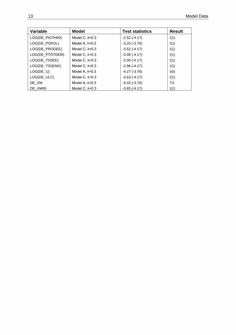
13 Model Data

Variable Model Test statistics Result LOG(DE_PIOTH00) Model C, λ=0.3 -2.52 (-4.17) I(1) LOG(DE_POPUL) Model A, λ=0.3 -3.20 (-3.76) I(1) LOG(DE_PRODEE) Model C, λ=0.3 -3.52 (-4.17) I(1) LOG(DE_PTOTDEM) Model C, λ=0.3 -3.08 (-4.17) I(1) LOG(DE_TSSEE) Model C, λ=0.3 -2.00 (-4.17) I(1) LOG(DE_TSSEM1) Model C, λ=0.3 -2.96 (-4.17) I(1) LOG(DE_U) Model A, λ=0.3 -4.27 (-3.76) I(0) LOG(DE_ULC) Model C, λ=0.3 -3.63 (-4.17) I(1) DE_XM Model A, λ=0.3 -4.02 (-3.76) TS DE_XM00 Model C, λ=0.3 -3.65 (-4.17) I(1)

Model Equations 14

3. Model Equations 3.1. Behavioural Equations 3.1.1. Real Aggregate Demand

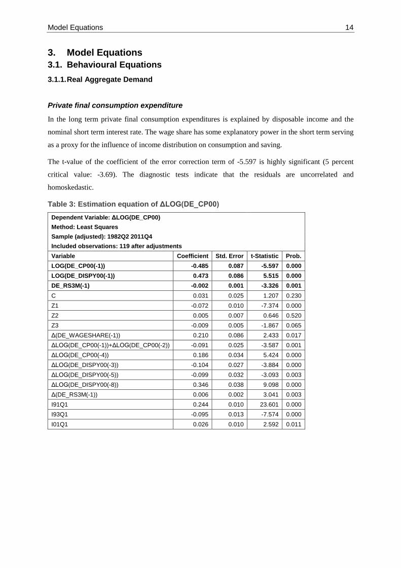
Private final consumption expenditure

In the long term private final consumption expenditures is explained by disposable income and the

nominal short term interest rate. The wage share has some explanatory power in the short term serving

as a proxy for the influence of income distribution on consumption and saving.

The t-value of the coefficient of the error correction term of -5.597 is highly significant (5 percent

critical value: -3.69). The diagnostic tests indicate that the residuals are uncorrelated and

homoskedastic.

Table 3: Estimation equation of ΔLOG(DE_CP00) Dependent Variable: ΔLOG(DE_CP00)

Method: Least Squares Sample (adjusted): 1982Q2 2011Q4

Included observations: 119 after adjustments Variable Coefficient Std. Error t-Statistic Prob.

LOG(DE_CP00(-1)) -0.485 0.087 -5.597 0.000 LOG(DE_DISPY00(-1)) 0.473 0.086 5.515 0.000 DE_RS3M(-1) -0.002 0.001 -3.326 0.001 C 0.031 0.025 1.207 0.230 Z1 -0.072 0.010 -7.374 0.000 Z2 0.005 0.007 0.646 0.520 Z3 -0.009 0.005 -1.867 0.065 Δ(DE_WAGESHARE(-1)) 0.210 0.086 2.433 0.017 ΔLOG(DE_CP00(-1))+ΔLOG(DE_CP00(-2)) -0.091 0.025 -3.587 0.001 ΔLOG(DE_CP00(-4)) 0.186 0.034 5.424 0.000 ΔLOG(DE_DISPY00(-3)) -0.104 0.027 -3.884 0.000 ΔLOG(DE_DISPY00(-5)) -0.099 0.032 -3.093 0.003 ΔLOG(DE_DISPY00(-8)) 0.346 0.038 9.098 0.000 Δ(DE_RS3M(-1)) 0.006 0.002 3.041 0.003 I91Q1 0.244 0.010 23.601 0.000 I93Q1 -0.095 0.013 -7.574 0.000 I01Q1 0.026 0.010 2.592 0.011

15 Model Equations

Table 4: Diagnostics of estimation equation of ΔLOG(DE_CP00) Adjusted R2 0.96 Residual tests Normality test (Jarque-Bera) 0.97 Serial correlation LM test (lag 1) 0.11 Serial correlation LM test (lag 4) 0.51 Serial correlation LM test (lag 8) 0.36 ARCH LM test (lag 1) 0.36 ARCH LM test (lag 4) 0.17 White's heteroskedasticity test 0.12 RESET test (h=2) 0.01

Stability tests Number of observations outside error bands

CUSUM test 0 CUSUM of squares test 3

Government consumption expenditure

The long-term evolution of government consumption is explained by past real GDP excluding

government consumption. Due to structural breaks two step dummies are included in the error

correction term. With a t-value of -3.105 the coefficient of the error-correction term is not significant

(5 percent critical value: -3.91)

Table 5: Estimation equation of ΔLOG(DE_CGOV00) Dependent Variable: ΔLOG(DE_CGOV00)

Method: Least Squares Sample (adjusted): 1982Q2 2011Q4 Included observations: 119 after adjustments Variable Coefficient Std. Error t-Statistic Prob.

LOG(DE_CGOV00(-1)) -0.109 0.035 -3.105 0.003 LOG(DE_GDP00(-8)-DE_CGOV00(-8)) 0.046 0.022 2.108 0.037 S91Q1 0.026 0.008 3.410 0.001 S09Q1 0.008 0.004 2.120 0.036 C 0.197 0.065 3.060 0.003 Z1 -0.037 0.006 -6.003 0.000 Z2 -0.024 0.004 -5.813 0.000 Z3 -0.018 0.004 -4.261 0.000 ΔLOG(DE_GDP00(-2)) 0.103 0.035 2.907 0.005 ΔLOG(DE_CGOV00(-4)) 0.598 0.067 8.908 0.000 ΔLOG(DE_CGOV00(-8)) -0.154 0.044 -3.514 0.001 I89Q1 -0.034 0.009 -3.621 0.001 I90Q1 0.042 0.009 4.452 0.000 I91Q1 0.124 0.012 10.591 0.000 I92Q1 -0.102 0.014 -7.083 0.000 I95Q1 -0.050 0.009 -5.442 0.000

The diagnostic tests show that the residuals are well-behaved and the estimation is stable over the

sample.

Model Equations 16

Table 6: Diagnostics of estimation equation of ΔLOG(DE_CGOV00)

Adjusted R2 0.94 Residual tests

Normality test (Jarque-Bera) 0.51 Serial correlation LM test (lag 1) 0.34 Serial correlation LM test (lag 4) 0.52 Serial correlation LM test (lag 8) 0.13 ARCH LM test (lag 1) 0.94 ARCH LM test (lag 4) 0.76 White's heteroskedasticity test 0.29 RESET test (h=2) 0.11



Gross fixed capital formation: machinery and equipment

Table 7: Estimation equation of ΔLOG(DE_IMEQ00) Dependent Variable: ΔLOG(DE_IMEQ00)

Method: Least Squares Sample (adjusted): 1982Q3 2011Q4 Included observations: 118 after adjustments

Variable Coefficient Std. Error t-Statistic Prob. LOG(DE_IMEQ00(-1)) -0.107 0.031 -3.422 0.001 LOG(DE_GDP00(-1)+DE_M00(-1)) 0.056 0.030 1.873 0.064 DE_RL10Y(-1) -0.010 0.002 -4.651 0.000 C 0.079 0.114 0.690 0.492 Z1 -0.387 0.033 -11.555 0.000 Z2 -0.052 0.033 -1.608 0.111 Z3 -0.108 0.039 -2.770 0.007 Z1*S91Q1 0.124 0.014 8.795 0.000 Z2*S91Q1 0.060 0.013 4.699 0.000 Z3*S91Q1 0.085 0.015 5.659 0.000 ΔLOG(DE_CAPA) 1.026 0.168 6.127 0.000 ΔLOG(DE_ULC00(-3)) +ΔLOG(DE_ULC00(-6)) -0.245 0.123 -1.986 0.050

ΔLOG(DE_IMEQ00(-2)) 0.288 0.053 5.399 0.000 ΔLOG(DE_IMEQ00(-3)) -0.102 0.062 -1.656 0.101 ΔLOG(DE_GDP00(-3)+ DE_M00(-3)) +ΔLOG(DE_GDP00(-5)+DE_M00(-5)) 0.155 0.094 1.649 0.103

Δ(DE_RL10Y(-1)) +Δ(DE_RL10Y(-5)) +Δ(DE_RL10Y(-4)) +Δ(DE_RL10Y(-9)) 0.016 0.004 3.553 0.001

I83Q1 0.036 0.021 1.705 0.092 I83Q2 0.045 0.021 2.099 0.039 I84Q2 -0.062 0.022 -2.857 0.005 I84Q3 0.122 0.022 5.545 0.000 I91Q1 0.113 0.023 4.827 0.000 I01Q2 -0.046 0.021 -2.233 0.028 I07Q4 0.057 0.021 2.764 0.007 I09Q1 -0.149 0.022 -6.836 0.000

17 Model Equations

In the long run investment into machinery and equipment is determined by total demand and the long-

term nominal interest rate. The coefficient of the error-correction term is significant at the 10 percent

level (10 percent critical value: -3.39, 5 percent critical value: -3.69).

The estimated equation passes all diagnostic tests.

Table 8: Diagnostics of estimation equation of ΔLOG(DE_IMEQ00) Adjusted R2 0.99 Residual tests Normality test (Jarque-Bera) 0.84 Serial correlation LM test (lag 1) 0.85 Serial correlation LM test (lag 4) 0.47 Serial correlation LM test (lag 8) 0.47 ARCH LM test (lag 1) 0.21 ARCH LM test (lag 4) 0.46 White's heteroskedasticity test 0.75 RESET test (h=2) 0.95



Gross fixed capital formation: private residential construction

In the long term private residential construction is explained by the population, the real long-term

interest rate and a step dummy. With a t-value of -7.298 the coefficient of the error-correction term is

highly significant (5 percent critical value: -3.91).

Table 9: Estimation equation of ΔLOG(DE_ID00) Dependent Variable: ΔLOG(DE_ID00)



LOG(DE_ID00(-1)) -0.315 0.043 -7.298 0.000 LOG(DE_POPUL(-1)) 0.463 0.077 6.015 0.000 DE_RL10Y00(-3) -0.005 0.001 -3.409 0.001 S02Q1 -0.058 0.010 -5.644 0.000 C -4.098 0.725 -5.653 0.000 Z1 -0.062 0.009 -6.591 0.000 Z2 0.148 0.021 6.970 0.000 Z3 0.080 0.010 8.329 0.000 ΔLOG(DE_ID00(-4)) 0.294 0.059 4.952 0.000 ΔLOG(DE_PID00(-1)) -1.477 0.363 -4.070 0.000 I85Q1 -0.181 0.028 -6.496 0.000 I86Q1 -0.123 0.030 -4.145 0.000 I87Q1 -0.162 0.029 -5.578 0.000 I91Q1 0.125 0.029 4.366 0.000 I05Q1 -0.096 0.028 -3.458 0.001

Model Equations 18

Table 10: Diagnostics of estimation equation of ΔLOG(DE_ID00) Adjusted R2 0.97 Residual tests Normality test (Jarque-Bera) 0.19 Serial correlation LM test (lag 1) 0.61 Serial correlation LM test (lag 4) 0.63 Serial correlation LM test (lag 8) 0.52 ARCH LM test (lag 1) 0.81 ARCH LM test (lag 4) 0.10 White's heteroskedasticity test 0.05 RESET test (h=2) 0.35



The estimation equation passes most diagnostic tests. There is some indication of heteroskedasticity.

Gross fixed capital formation: private non-residential construction

There is a highly significant long-term relationship between private non-residential construction and

domestic final demand, although some structural changes in this relationship have to be modelled with

dummy variables. With a t-statistic of -6.038 the coefficient of the error-correction term is highly

significant (5 percent critical value: -3.91).

Table 11: Estimation equation of ΔLOG(DE_INRB00)

Dependent Variable: ΔLOG(DE_INRB00) Method: Least Squares

Sample (adjusted): 1981Q2 2011Q4 Included observations: 123 after adjustments

Variable Coefficient Std. Error t-Statistic Prob. LOG(DE_INRB00(-1)) -0.419 0.069 -6.038 0.000 LOG(DE_IEND00(-1)) 0.471 0.084 5.608 0.000 S02Q1*LOG(@TREND) -0.012 0.003 -3.618 0.001 1-S98Q1 0.097 0.018 5.262 0.000 C -1.748 0.335 -5.218 0.000 Z1 -0.087 0.020 -4.336 0.000 Z2 0.146 0.030 4.960 0.000 Z3 0.061 0.016 3.682 0.000 I91Q1 0.174 0.036 4.857 0.000 Z1*S91Q1 0.052 0.022 2.401 0.018 Z2*S91Q1 -0.028 0.021 -1.331 0.186 Z3*S91Q1 0.011 0.019 0.604 0.547 ΔLOG(DE_INRB00(-4)) 0.296 0.065 4.565 0.000 I85Q1 -0.152 0.037 -4.097 0.000 I87Q1 -0.134 0.037 -3.608 0.001 I96Q1 -0.128 0.036 -3.541 0.001 I05Q1 -0.110 0.036 -3.063 0.003

19 Model Equations

Except for some heteroskedasticity the residuals are well-behaved and the estimation is stable over the

sample period.

Table 12: Diagnostics of estimation equation of ΔLOG(DE_INRB00) Adjusted R2 0.94 Residual tests Normality test (Jarque-Bera) 0.49 Serial correlation LM test (lag 1) 0.66 Serial correlation LM test (lag 4) 0.46 Serial correlation LM test (lag 8) 0.52 ARCH LM test (lag 1) 0.99 ARCH LM test (lag 4) 0.34 White's heteroskedasticity test 0.02 RESET test (h=2) 0.06



Other gross fixed capital formation

The long-term evolution of other gross fixed capital formation is explained by real exports and a linear

trend starting in 1970. With a t-statistic of -4.225 the coefficient of the error-correction term is highly

significant (5 percent critical value: -3.69).

Table 13: Estimation equation of ΔLOG(DE_IOTH00) Dependent Variable: ΔLOG(DE_IOTH00)



LOG(DE_IOTH00(-1)) -0.151 0.036 -4.225 0.000 LOG(DE_X00(-1)) 0.034 0.014 2.363 0.020 LOG(@TREND(1970:1)) 0.208 0.051 4.115 0.000 C -0.935 0.226 -4.133 0.000 Z1 -0.058 0.011 -5.145 0.000 Z2 -0.025 0.005 -4.634 0.000 Z3 -0.034 0.007 -4.597 0.000 ΔLOG(DE_IOTH00(-4)) 0.576 0.080 7.197 0.000 ΔLOG(DE_IOTH00(-8)) 0.172 0.081 2.118 0.037 ΔLOG(DE_X00(-3)) 0.103 0.044 2.378 0.019 ΔLOG(DE_X00(-4)) -0.114 0.045 -2.546 0.012 I86Q4 -0.066 0.018 -3.726 0.000

The specification passes all diagnostic tests at the 5 percent level.

Model Equations 20

Table 14: Diagnostics of estimation equation of ΔLOG(DE_IOTH00) Adjusted R2 0.93 Residual tests Normality test (Jarque-Bera) 0.11 Serial correlation LM test (lag 1) 0.56 Serial correlation LM test (lag 4) 0.78 Serial correlation LM test (lag 8) 0.89 ARCH LM test (lag 1) 0.09 ARCH LM test (lag 4) 0.17 White's heteroskedasticity test 0.15 RESET test (h=2) 0.24



Changes in inventories and net acquisition of valuables

No error-correction equation is estimated, because the variable is stationary. It is explained by its own lagged observations and some deterministics, making it in fact an exogenous variable.

Table 15: Estimation equation of DE_INV00 Dependent Variable: DE_INV00



C 0.938 0.434 2.161 0.033 Z1*@TREND 0.041 0.024 1.693 0.093 Z2*@TREND 0.029 0.013 2.219 0.029 Z3*@TREND -0.001 0.023 -0.038 0.970 DE_INV00(-1) 0.153 0.079 1.921 0.057 DE_INV00(-3) -0.213 0.056 -3.781 0.000 DE_INV00(-4) 0.642 0.059 10.882 0.000 DE_INV00(-5) -0.251 0.075 -3.342 0.001 I91Q1 12.753 2.592 4.920 0.000 I91Q2 6.732 2.759 2.440 0.016 I91Q3 9.136 2.688 3.399 0.001 I06Q4 -10.899 2.683 -4.063 0.000 I09Q2 -8.880 2.657 -3.343 0.001 S91Q1 1.449 0.558 2.598 0.011

The diagnostic tests indicate autoregressive conditional heteroskedasticity as well as limited stability over the sample period.

21 Model Equations

Table 16: Diagnostics of estimation equation of DE_INV00 Adjusted R2 0.93 Residual tests Normality test (Jarque-Bera) 0.65 Serial correlation LM test (lag 1) 0.87 Serial correlation LM test (lag 4) 0.84 Serial correlation LM test (lag 8) 0.59 ARCH LM test (lag 1) 0.68 ARCH LM test (lag 4) 0.00 White's heteroskedasticity test 0.45 RESET test (h=2) 0.92



Exports of goods to the euro area

In the long run real exports of goods to the euro area are explained by gross fixed capital formation in other euro area countries, the real exchange rate based on unit labour costs and a trend representing increasing economic integration. With a t-statistic of -8.174 the coefficient of the error-correction term is highly significant (5 percent critical value: -3.91)

Table 17: Estimation equation of ΔLOG(DE_XG00_EWU) Dependent Variable: ΔLOG(DE_XG00_EWU)



LOG(DE_XG00_EWU(-1)) -0.789 0.096 -8.174 0.000 LOG(EWU_ODE_IFC00(-1)) 0.551 0.084 6.563 0.000 LOG(DE_NEV_EWU(-1)*DE_ULC(-1)*100/EWU6_ULC(-1)) -0.539 0.071 -7.577 0.000 @TREND 0.004 0.001 8.111 0.000 C 2.881 0.394 7.314 0.000 Z1 0.022 0.054 0.402 0.689 Z2 -0.062 0.016 -3.939 0.000 Z3 -0.029 0.050 -0.580 0.563 ΔLOG(DE_XG00_EWU(-1)) 0.154 0.089 1.732 0.086 ΔLOG(DE_XG00_EWU(-2)) 0.102 0.082 1.247 0.215 ΔLOG(DE_XG00_EWU(-4)) 0.189 0.079 2.399 0.018 ΔLOG(EWU_ODE_IFC00) 0.823 0.124 6.652 0.000 ΔLOG(EWU_ODE_IFC00(-1)) 0.389 0.146 2.668 0.009 ΔLOG(EWU_ODE_IFC00(-2)) 0.603 0.139 4.351 0.000 ΔLOG(EWU_ODE_IFC00(-3)) 0.324 0.137 2.356 0.020 ΔLOG(DE_NEV_EWU*DE_ULC*100/EWU6_ULC) -0.427 0.134 -3.176 0.002

The specification passes all diagnostic tests. The residuals are well-behaved and the estimated equation is stable over the sample period.

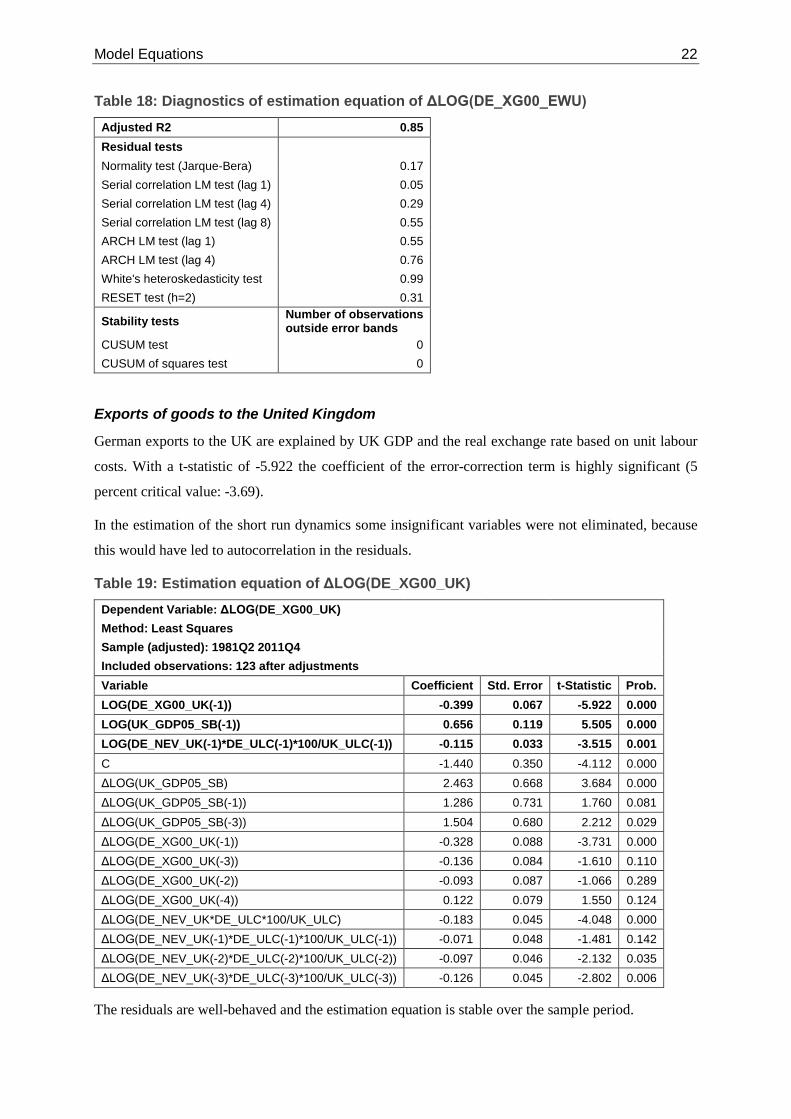
Model Equations 22

Table 18: Diagnostics of estimation equation of ΔLOG(DE_XG00_EWU) Adjusted R2 0.85 Residual tests Normality test (Jarque-Bera) 0.17 Serial correlation LM test (lag 1) 0.05 Serial correlation LM test (lag 4) 0.29 Serial correlation LM test (lag 8) 0.55 ARCH LM test (lag 1) 0.55 ARCH LM test (lag 4) 0.76 White's heteroskedasticity test 0.99 RESET test (h=2) 0.31



Exports of goods to the United Kingdom

German exports to the UK are explained by UK GDP and the real exchange rate based on unit labour

costs. With a t-statistic of -5.922 the coefficient of the error-correction term is highly significant (5

percent critical value: -3.69).

In the estimation of the short run dynamics some insignificant variables were not eliminated, because

this would have led to autocorrelation in the residuals.

Table 19: Estimation equation of ΔLOG(DE_XG00_UK) Dependent Variable: ΔLOG(DE_XG00_UK)


LOG(DE_XG00_UK(-1)) -0.399 0.067 -5.922 0.000 LOG(UK_GDP05_SB(-1)) 0.656 0.119 5.505 0.000 LOG(DE_NEV_UK(-1)*DE_ULC(-1)*100/UK_ULC(-1)) -0.115 0.033 -3.515 0.001 C -1.440 0.350 -4.112 0.000 ΔLOG(UK_GDP05_SB) 2.463 0.668 3.684 0.000 ΔLOG(UK_GDP05_SB(-1)) 1.286 0.731 1.760 0.081 ΔLOG(UK_GDP05_SB(-3)) 1.504 0.680 2.212 0.029 ΔLOG(DE_XG00_UK(-1)) -0.328 0.088 -3.731 0.000 ΔLOG(DE_XG00_UK(-3)) -0.136 0.084 -1.610 0.110 ΔLOG(DE_XG00_UK(-2)) -0.093 0.087 -1.066 0.289 ΔLOG(DE_XG00_UK(-4)) 0.122 0.079 1.550 0.124 ΔLOG(DE_NEV_UK*DE_ULC*100/UK_ULC) -0.183 0.045 -4.048 0.000 ΔLOG(DE_NEV_UK(-1)*DE_ULC(-1)*100/UK_ULC(-1)) -0.071 0.048 -1.481 0.142 ΔLOG(DE_NEV_UK(-2)*DE_ULC(-2)*100/UK_ULC(-2)) -0.097 0.046 -2.132 0.035 ΔLOG(DE_NEV_UK(-3)*DE_ULC(-3)*100/UK_ULC(-3)) -0.126 0.045 -2.802 0.006

The residuals are well-behaved and the estimation equation is stable over the sample period.

23 Model Equations

Table 20: Estimation equation of ΔLOG(DE_XG00_UK) Adjusted R2 0.49 Residual tests Normality test (Jarque-Bera) 0.45 Serial correlation LM test (lag 1) 0.26 Serial correlation LM test (lag 4) 0.09 Serial correlation LM test (lag 8) 0.34 ARCH LM test (lag 1) 0.61 ARCH LM test (lag 4) 0.78 White's heteroskedasticity test 0.17 RESET test (h=2) 0.31 Stability tests outside error bands CUSUM test 0 CUSUM of squares test 0

Exports of goods to the United States of America

German exports of goods to the USA are determined in the long run by US gross fixed capital

formation, the real exchange rate based on unit labour costs and a trend. With a t-statistic of -5.691

error-correction coefficient is highly significant (5 percent critical value: -3.91)

Table 21: Estimation equation of ΔLOG(DE_XG00_US) Dependent Variable: ΔLOG(DE_XG00_US)



LOG(DE_XG00_US(-1)) -0.322 0.057 -5.691 0.000 LOG(US_IFC00(-1)) 0.235 0.081 2.919 0.004 LOG(DE_NEV_US(-1) *DE_ULC(-1) *100/US_ULC(-1)) -0.337 0.046 -7.391 0.000 @TREND 0.002 0.000 4.945 0.000 C 0.850 0.241 3.526 0.001 Z1 -0.078 0.029 -2.642 0.010 Z2 -0.096 0.019 -5.059 0.000 Z3 -0.063 0.019 -3.277 0.001 ΔLOG(DE_XG00_US(-1)) -0.277 0.070 -3.937 0.000 ΔLOG(DE_XG00_US(-2)) -0.181 0.081 -2.243 0.027 ΔLOG(DE_XG00_US(-3)) -0.244 0.070 -3.491 0.001 ΔLOG(DE_XG00_US(-5)) -0.184 0.064 -2.891 0.005 ΔLOG(US_IFC00) 1.241 0.269 4.616 0.000 ΔLOG(US_IFC00(-2)) 1.426 0.344 4.148 0.000 ΔLOG(US_IFC00(-4)) 0.635 0.296 2.147 0.034 ΔLOG(DE_NEV_US *DE_ULC*100/US_ULC) -0.264 0.089 -2.949 0.004 I84Q2 -0.190 0.050 -3.807 0.000

The specification passes all diagnostic tests.

Model Equations 24

Table 22: Diagnostics of estimation equation of ΔLOG(DE_XG00_US) Adjusted R2 0.70 Residual tests Normality test (Jarque-Bera) 0.84 Serial correlation LM test (lag 1) 0.16 Serial correlation LM test (lag 4) 0.17 Serial correlation LM test (lag 8) 0.27 ARCH LM test (lag 1) 0.66 ARCH LM test (lag 4) 0.28 White's heteroskedasticity test 0.63 RESET test (h=2) 0.84



Exports of goods to the rest of the world

The long-term evolution of exports to the rest of the world is explained by real GDP in the rest of the

world and the real effective exchange rate in terms of the CPI vis-à-vis 56 countries. With a t-statistic

of -5.064 the error-correction coefficient is highly significant (5 percent critical value: -3.69). Short-

run dynamics of exports of goods to the rest of the world are determined by foreign demand.

Table 23: Estimation equation of ΔLOG(DE_XG00_ROW) Dependent Variable: ΔLOG(DE_XG00_ROW)

Method: Least Squares Sample: 1988Q1 2011Q4 Included observations: 96 Variable Coefficient Std. Error t-Statistic Prob.

LOG(DE_XG00_ROW(-1)) -0.430 0.085 -5.064 0.000 LOG(ROW_GDP00(-1)) 0.914 0.185 4.944 0.000 LOG(DE_REEV_56_CPI(-1)) -0.395 0.124 -3.180 0.002 C -0.719 0.610 -1.179 0.242 Z1 -0.099 0.014 -7.183 0.000 Z2 -0.027 0.013 -1.991 0.050 Z3 -0.018 0.013 -1.409 0.163 ΔLOG(ROW_GDP00) 1.291 0.747 1.730 0.087 ΔLOG(ROW_GDP00(-1)) 2.446 0.701 3.487 0.001 ΔLOG(ROW_GDP00(-5)) 1.604 0.719 2.231 0.028 I90Q4 0.186 0.048 3.849 0.000 I91Q1 -0.117 0.053 -2.222 0.029

The residuals pass all diagnostic tests and the specification is stable over the sample period.

25 Model Equations

Table 24: Diagnostics of estimation equation of ΔLOG(DE_XG00_ROW) Adjusted R2 0.67 Residual tests Normality test (Jarque-Bera) 0.23 Serial correlation LM test (lag 1) 0.73 Serial correlation LM test (lag 4) 0.29 Serial correlation LM test (lag 8) 0.53 ARCH LM test (lag 1) 0.72 ARCH LM test (lag 4) 0.70 White's heteroskedasticity test 0.43 RESET test (h=2) 0.49



Exports of services

Exports of services include a large number of services which are somehow connected to exports of

goods such as transport or insurance. Therefore it is not surprising that long-term service exports are

linked to goods exports. The t-statistic of -4.495 indicates that the error-correction coefficient is highly

significant (5 percent critical value: -3.41). The real effective exchange rate vis-à-vis 24 countries

(based on the total demand deflator) plays an important role for the short-term dynamics.

Table 25: Estimation equation of ΔLOG(DE_XS00) Dependent Variable: ΔLOG(DE_XS00)


Variable Coefficient Std. Error t-Statistic Prob. LOG(DE_XS00(-1)) -0.234 0.052 -4.495 0.000 LOG(DE_XG00(-1)) 0.233 0.050 4.636 0.000 C -0.397 0.090 -4.431 0.000 Z1 -0.155 0.016 -9.767 0.000 Z2 -0.048 0.014 -3.378 0.001 Z3 -0.023 0.015 -1.542 0.126 ΔLOG(DE_XS00(-1)) -0.248 0.051 -4.839 0.000 ΔLOG(DE_XG00(-4)) -0.206 0.112 -1.836 0.069 ΔLOG(DE_REEV_24_PTOTDEM) -0.714 0.322 -2.216 0.029 ΔLOG(DE_REEV_24_PTOTDEM(-1)) -1.096 0.313 -3.501 0.001 ΔLOG(DE_REEV_24_PTOTDEM(-3)) 0.681 0.315 2.159 0.033 ΔLOG(DE_REEV_24_PTOTDEM(-6)) -0.527 0.279 -1.890 0.062 I90Q1 0.181 0.043 4.259 0.000 I90Q3 0.380 0.043 8.834 0.000 I90Q4 0.234 0.049 4.774 0.000 I91Q1 -0.450 0.048 -9.421 0.000 I99Q1 -0.199 0.043 -4.595 0.000 I01Q4 0.177 0.043 4.114 0.000

Model Equations 26

The diagnostics reveal some serial correlation, which could not be eliminated despite the inclusion of

lagged dependent variables.

Table 26: Diagnostics of estimation equation of ΔLOG(DE_XS00) Adjusted R2 0.88 Residual tests Normality test (Jarque-Bera) 0.64 Serial correlation LM test (lag 1) 0.09 Serial correlation LM test (lag 4) 0.02 Serial correlation LM test (lag 8) 0.15 ARCH LM test (lag 1) 0.33 ARCH LM test (lag 4) 0.18 White's heteroskedasticity test 0.30 RESET test (h=2) 0.13



Imports of goods Table 27: Estimation equation of ΔLOG(DE_MG00)

Dependent Variable: ΔLOG(DE_MG00) Method: Least Squares

Sample (adjusted): 1981Q3 2011Q4 Included observations: 122 after adjustments Variable Coefficient Std. Error t-Statistic Prob.

LOG(DE_MG00(-1)) -0.468 0.075 -6.224 0.000 LOG(DE_PMGREL(-1)) -0.206 0.037 -5.618 0.000 LOG(DE_XG00(-1)) 0.277 0.043 6.407 0.000 LOG(DE_IMEQ00(-1)) 0.126 0.037 3.396 0.001 (S91Q1)*@TREND 0.001 0.000 4.504 0.000 C 1.283 0.219 5.863 0.000 Z1 -0.043 0.025 -1.720 0.088 Z2 -0.029 0.015 -1.955 0.053 Z3 -0.071 0.023 -3.080 0.003 ΔLOG(DE_XG00) 0.410 0.059 6.968 0.000 ΔLOG(DE_XG00(-3)) -0.140 0.058 -2.400 0.018 ΔLOG(DE_XG00(-5)) -0.104 0.055 -1.894 0.061 ΔLOG(DE_CP00(-1)) 0.265 0.067 3.984 0.000 ΔLOG(DE_IMEQ00) 0.182 0.054 3.379 0.001 ΔLOG(DE_IMEQ00(-3)) 0.185 0.055 3.341 0.001 ΔLOG(DE_MG00(-2)) 0.111 0.059 1.869 0.064 I93Q1 -0.084 0.022 -3.810 0.000 I05Q1 -0.066 0.021 -3.147 0.002

In the long run imports of goods depend on the prices of imported goods relative to the domestic price

level, exports of goods and investment into machinery and equipment. They rise with increasing

economic integration, which is represented by a trend beginning in 1991 in this equation. The error-

27 Model Equations

correction coefficient is highly significant with a t-statistic of -6.224 (5 percent critical value: -4.12).

In the short run changes of private consumption also play a role.

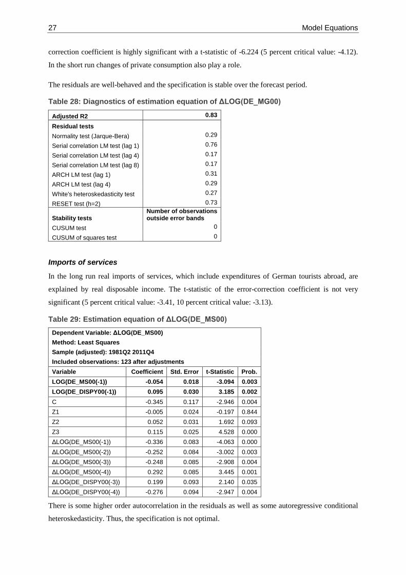
The residuals are well-behaved and the specification is stable over the forecast period.

Table 28: Diagnostics of estimation equation of ΔLOG(DE_MG00)

Adjusted R2 0.83

Residual tests Normality test (Jarque-Bera) 0.29

Serial correlation LM test (lag 1) 0.76



ARCH LM test (lag 1) 0.31

ARCH LM test (lag 4) 0.29

White's heteroskedasticity test 0.27

RESET test (h=2) 0.73


CUSUM test 0

CUSUM of squares test 0

Imports of services

In the long run real imports of services, which include expenditures of German tourists abroad, are

explained by real disposable income. The t-statistic of the error-correction coefficient is not very

significant (5 percent critical value: -3.41, 10 percent critical value: -3.13).

Table 29: Estimation equation of ΔLOG(DE_MS00) Dependent Variable: ΔLOG(DE_MS00)



LOG(DE_MS00(-1)) -0.054 0.018 -3.094 0.003 LOG(DE_DISPY00(-1)) 0.095 0.030 3.185 0.002 C -0.345 0.117 -2.946 0.004 Z1 -0.005 0.024 -0.197 0.844 Z2 0.052 0.031 1.692 0.093 Z3 0.115 0.025 4.528 0.000 ΔLOG(DE_MS00(-1)) -0.336 0.083 -4.063 0.000 ΔLOG(DE_MS00(-2)) -0.252 0.084 -3.002 0.003 ΔLOG(DE_MS00(-3)) -0.248 0.085 -2.908 0.004 ΔLOG(DE_MS00(-4)) 0.292 0.085 3.445 0.001 ΔLOG(DE_DISPY00(-3)) 0.199 0.093 2.140 0.035 ΔLOG(DE_DISPY00(-4)) -0.276 0.094 -2.947 0.004

There is some higher order autocorrelation in the residuals as well as some autoregressive conditional

heteroskedasticity. Thus, the specification is not optimal.

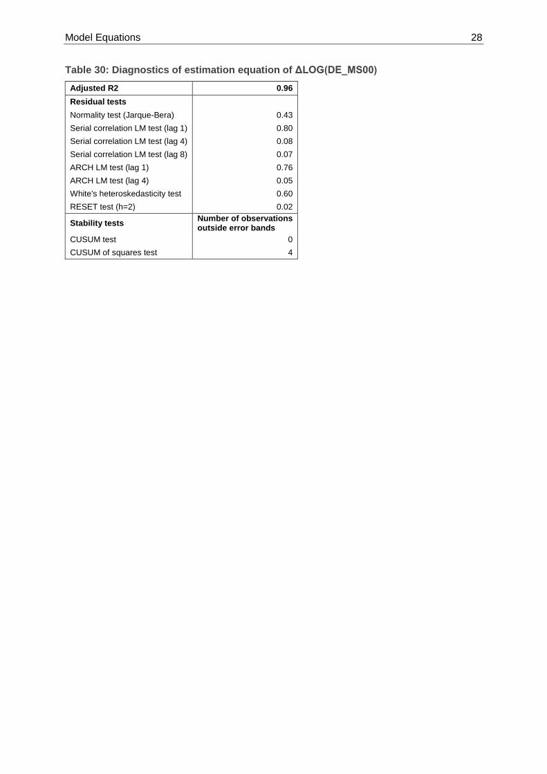
Model Equations 28

Table 30: Diagnostics of estimation equation of ΔLOG(DE_MS00) Adjusted R2 0.96 Residual tests Normality test (Jarque-Bera) 0.43 Serial correlation LM test (lag 1) 0.80 Serial correlation LM test (lag 4) 0.08 Serial correlation LM test (lag 8) 0.07 ARCH LM test (lag 1) 0.76 ARCH LM test (lag 4) 0.05 White's heteroskedasticity test 0.60 RESET test (h=2) 0.02



29 Model Equations

3.1.2. Prices and Exchange Rates

Private consumption deflator

In the long term the private consumption deflator is explained by unit labour costs, the price level

(CPI) in the euro area and the oil price in euro terms. The error-correction coefficient is highly

significant with a t-statistic of -7.250 (5 percent critical value: -3.91).

Table 31: Estimation equation of ΔLOG(DE_PCP00) Dependent Variable: ΔLOG(DE_PCP00)


LOG(DE_PCP00(-1)) -0.159 0.022 -7.250 0.000 LOG(DE_ULC(-1)) 0.040 0.011 3.605 0.001 LOG(CPI_EWU(-1)) 0.079 0.011 7.201 0.000 LOG(OIL$(-1)/DE_NEV_US(-1)/100) 0.003 0.001 2.295 0.024 C 0.406 0.074 5.514 0.000 Z1 -0.024 0.005 -5.234 0.000 Z2 -0.010 0.002 -4.795 0.000 Z3 -0.009 0.002 -4.146 0.000 ΔLOG(DE_PCP00(-4)) 0.131 0.025 5.173 0.000 ΔLOG(DE_PM00) 0.086 0.020 4.345 0.000 ΔLOG(DE_PM00(-1)) -0.107 0.018 -5.952 0.000 ΔLOG(DE_ULC(-4)) -0.064 0.018 -3.643 0.000 ΔLOG(CPI_EWU) 0.535 0.084 6.338 0.000 ΔLOG(CPI_EWU(-1)) 0.423 0.089 4.744 0.000 I91Q1 -0.050 0.003 -15.935 0.000


Table 32: Diagnostics of Estimation equation of ΔLOG(DE_PCP00) Adjusted R2 0.86 Residual tests Normality test (Jarque-Bera) 0.25 Serial correlation LM test (lag 1) 0.95 Serial correlation LM test (lag 4) 0.42 Serial correlation LM test (lag 8) 0.60 ARCH LM test (lag 1) 0.62 ARCH LM test (lag 4) 0.34 White's heteroskedasticity test 0.13 RESET test (h=2) 0.25



Model Equations 30

Government consumption deflator

The government consumption deflator is determined by the wage level and the GDP deflator in the

long run. A step dummy is included in the error-correction term to account for German reunification.

With a t-statistic of -7.798 the error-correction coefficient is highly significant (5 percent critical

value: -3.91).

Table 33: Estimation equation of ΔLOG(DE_PCGOV00) Dependent Variable: ΔLOG(DE_PCGOV00)



LOG(DE_PCGOV00(-1)) -0.610 0.078 -7.798 0.000 LOG(DE_GWAGE(-1)) 0.192 0.029 6.574 0.000 LOG(DE_PGDP00(-1)) 0.273 0.069 3.943 0.000 S91Q1 -0.040 0.006 -6.214 0.000 C 0.548 0.112 4.908 0.000 Z1 -0.041 0.010 -4.086 0.000 Z2 -0.017 0.006 -2.752 0.007 Z3 -0.007 0.009 -0.842 0.402 Z1*(1-S91Q1) -0.017 0.006 -2.726 0.008 Z2*(1-S91Q1) -0.013 0.005 -2.528 0.013 Z3*(1-S91Q1) -0.005 0.006 -0.852 0.396 ΔLOG(DE_PCGOV00(-3)) -0.131 0.050 -2.607 0.011 ΔLOG(DE_PCGOV00(-4)) 0.387 0.078 4.969 0.000 ΔLOG(DE_PCGOV00(-8)) 0.157 0.066 2.395 0.018 I91Q2 0.038 0.009 4.013 0.000 I92Q2 -0.020 0.009 -2.168 0.033 I92Q3 0.031 0.009 3.616 0.001


Table 34: Diagnostics of Estimation equation of ΔLOG(DE_PCGOV00) Adjusted R2 0.99 Residual tests Normality test (Jarque-Bera) 0.93 Serial correlation LM test (lag 1) 0.69 Serial correlation LM test (lag 4) 0.49 Serial correlation LM test (lag 8) 0.10 ARCH LM test (lag 1) 0.18 ARCH LM test (lag 4) 0.21 White's heteroskedasticity test 0.51 RESET test (h=2) 0.17



31 Model Equations

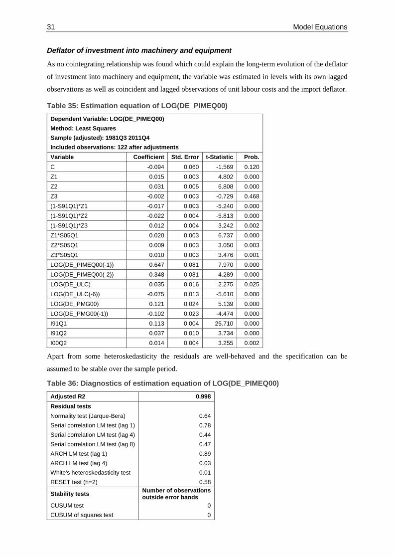
Deflator of investment into machinery and equipment

As no cointegrating relationship was found which could explain the long-term evolution of the deflator

of investment into machinery and equipment, the variable was estimated in levels with its own lagged

observations as well as coincident and lagged observations of unit labour costs and the import deflator.

Table 35: Estimation equation of LOG(DE_PIMEQ00) Dependent Variable: LOG(DE_PIMEQ00)



C -0.094 0.060 -1.569 0.120 Z1 0.015 0.003 4.802 0.000 Z2 0.031 0.005 6.808 0.000 Z3 -0.002 0.003 -0.729 0.468 (1-S91Q1)*Z1 -0.017 0.003 -5.240 0.000 (1-S91Q1)*Z2 -0.022 0.004 -5.813 0.000 (1-S91Q1)*Z3 0.012 0.004 3.242 0.002 Z1*S05Q1 0.020 0.003 6.737 0.000 Z2*S05Q1 0.009 0.003 3.050 0.003 Z3*S05Q1 0.010 0.003 3.476 0.001 LOG(DE_PIMEQ00(-1)) 0.647 0.081 7.970 0.000 LOG(DE_PIMEQ00(-2)) 0.348 0.081 4.289 0.000 LOG(DE_ULC) 0.035 0.016 2.275 0.025 LOG(DE_ULC(-6)) -0.075 0.013 -5.610 0.000 LOG(DE_PMG00) 0.121 0.024 5.139 0.000 LOG(DE_PMG00(-1)) -0.102 0.023 -4.474 0.000 I91Q1 0.113 0.004 25.710 0.000 I91Q2 0.037 0.010 3.734 0.000 I00Q2 0.014 0.004 3.255 0.002

Apart from some heteroskedasticity the residuals are well-behaved and the specification can be

assumed to be stable over the sample period.

Table 36: Diagnostics of estimation equation of LOG(DE_PIMEQ00) Adjusted R2 0.998 Residual tests Normality test (Jarque-Bera) 0.64 Serial correlation LM test (lag 1) 0.78 Serial correlation LM test (lag 4) 0.44 Serial correlation LM test (lag 8) 0.47 ARCH LM test (lag 1) 0.89 ARCH LM test (lag 4) 0.03 White's heteroskedasticity test 0.01 RESET test (h=2) 0.58



Model Equations 32

Deflator of private residential construction investment

A long-run relationship has been established between the deflator of private residential construction

and the deflator of private non-residential construction. However, the t-statistic of the error-correction

coefficient is significant only at the 10 percent level (-3.13; 5 percent critical value: -3.41).

Table 37: Estimation equation of ΔLOG(DE_PID00) Dependent Variable: ΔLOG(DE_PID00)


LOG(DE_PID00(-1)) -0.143 0.045 -3.165 0.002 LOG(DE_PINRB00(-1)) 0.153 0.050 3.045 0.003 C -0.046 0.026 -1.798 0.075 Z1 -0.010 0.002 -3.979 0.000 Z2 0.013 0.002 6.171 0.000 Z3 -0.004 0.002 -1.539 0.127 Z1*S91Q1 0.014 0.003 5.126 0.000 Z2*S91Q1 -0.011 0.002 -4.444 0.000 Z3*S91Q1 0.005 0.003 1.784 0.077 ΔLOG(DE_PID00(-2)) 0.119 0.069 1.729 0.087 ΔLOG(DE_PINRB00(-1)) 0.268 0.065 4.100 0.000 ΔLOG(DE_PINRB00(-7)) 0.087 0.025 3.458 0.001 I90Q1 0.017 0.004 4.163 0.000 I91Q2 0.021 0.004 5.442 0.000 I07Q1 0.028 0.004 7.036 0.000

The specification does not pass all diagnostic tests. There is heteroskedasticity in the residuals and the

CUSUM of squares test points to instability.

Table 38: Diagnostics of Estimation equation of ΔLOG(DE_PID00) Adjusted R2 0.73 Residual tests Normality test (Jarque-Bera) 0.54 Serial correlation LM test (lag 1) 0.06 Serial correlation LM test (lag 4) 0.15 Serial correlation LM test (lag 8) 0.20 ARCH LM test (lag 1) 0.03 ARCH LM test (lag 4) 0.02 White's heteroskedasticity test 0.05 RESET test (h=2) 0.53



33 Model Equations

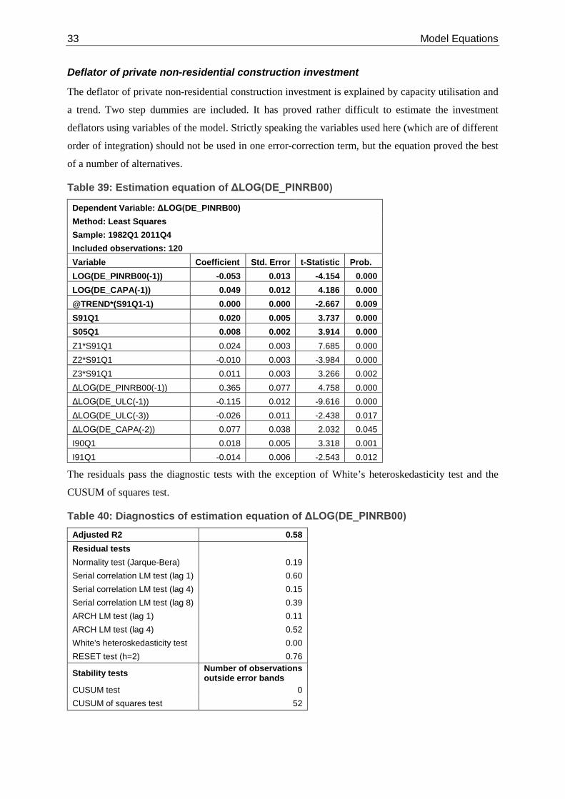
Deflator of private non-residential construction investment

The deflator of private non-residential construction investment is explained by capacity utilisation and

a trend. Two step dummies are included. It has proved rather difficult to estimate the investment

deflators using variables of the model. Strictly speaking the variables used here (which are of different

order of integration) should not be used in one error-correction term, but the equation proved the best

of a number of alternatives.

Table 39: Estimation equation of ΔLOG(DE_PINRB00)

Dependent Variable: ΔLOG(DE_PINRB00) Method: Least Squares

Sample: 1982Q1 2011Q4 Included observations: 120 Variable Coefficient Std. Error t-Statistic Prob.

LOG(DE_PINRB00(-1)) -0.053 0.013 -4.154 0.000 LOG(DE_CAPA(-1)) 0.049 0.012 4.186 0.000 @TREND*(S91Q1-1) 0.000 0.000 -2.667 0.009 S91Q1 0.020 0.005 3.737 0.000 S05Q1 0.008 0.002 3.914 0.000 Z1*S91Q1 0.024 0.003 7.685 0.000 Z2*S91Q1 -0.010 0.003 -3.984 0.000 Z3*S91Q1 0.011 0.003 3.266 0.002 ΔLOG(DE_PINRB00(-1)) 0.365 0.077 4.758 0.000 ΔLOG(DE_ULC(-1)) -0.115 0.012 -9.616 0.000 ΔLOG(DE_ULC(-3)) -0.026 0.011 -2.438 0.017 ΔLOG(DE_CAPA(-2)) 0.077 0.038 2.032 0.045 I90Q1 0.018 0.005 3.318 0.001 I91Q1 -0.014 0.006 -2.543 0.012

The residuals pass the diagnostic tests with the exception of White’s heteroskedasticity test and the

CUSUM of squares test.

Table 40: Diagnostics of estimation equation of ΔLOG(DE_PINRB00) Adjusted R2 0.58 Residual tests Normality test (Jarque-Bera) 0.19 Serial correlation LM test (lag 1) 0.60 Serial correlation LM test (lag 4) 0.15 Serial correlation LM test (lag 8) 0.39 ARCH LM test (lag 1) 0.11 ARCH LM test (lag 4) 0.52 White's heteroskedasticity test 0.00 RESET test (h=2) 0.76



Model Equations 34

Deflator of government construction investment

No cointegrating relationship could be found to explain the government construction deflator. It is

therefore estimated in levels being explained by its past observations as well as the coincident and

lagged observations of the deflator of private non-residential construction.

Table 41: Estimation equation of LOG(DE_PICONGOV00)

Dependent Variable: LOG(DE_PICONGOV00) Method: Least Squares

Sample (adjusted): 1981Q2 2011Q4 Included observations: 123 after adjustments Variable Coefficient Std. Error t-Statistic Prob.

C -0.010 0.009 -1.035 0.303 LOG(DE_PICONGOV00(-1)) 0.816 0.043 19.194 0.000 LOG(DE_PICONGOV00(-4)) 0.179 0.053 3.342 0.001 LOG(DE_PICONGOV00(-5)) -0.192 0.049 -3.872 0.000 LOG(DE_PINRB00) 0.823 0.053 15.649 0.000 LOG(DE_PINRB00(-1)) -0.637 0.066 -9.658 0.000 LOG(DE_PINRB00(-3)) 0.071 0.024 2.982 0.004 LOG(DE_PINRB00(-5)) -0.057 0.019 -3.012 0.003


Table 42: Diagnostics of estimation equation of LOG(DE_PICONGOV00) Adjusted R2 0.9996 Residual tests Normality test (Jarque-Bera) 0.85 Serial correlation LM test (lag 1) 0.09 Serial correlation LM test (lag 4) 0.36 Serial correlation LM test (lag 8) 0.61 ARCH LM test (lag 1) 0.85 ARCH LM test (lag 4) 0.39 White's heteroskedasticity test 0.13 RESET test (h=2) 0.09 Number of observations outside error bands

Number of observations outside error bands


Deflator of other gross fixed capital formation

Despite an insignificant error-correction coefficient the deflator of other gross fixed capital formation

has been estimated in an error-correction equation including the deflator of investment in machinery

and equipment and a broken trend. The equation shows a satisfactory in-sample forecast performance

and is the best option among several alternatives.

35 Model Equations

Table 43: Estimation equation of ΔLOG(DE_PIOTH00) Dependent Variable: ΔLOG(DE_PIOTH00)


LOG(DE_PIOTH00(-1)) -0.113 0.039 -2.872 0.005 LOG(DE_PIMEQ00(-1)) 0.101 0.030 3.400 0.001 @TREND 0.000 0.000 -2.986 0.004 (1-S94Q1)*@TREND 0.000 0.000 -2.248 0.027 C 0.093 0.077 1.208 0.230 Z1 0.002 0.003 0.624 0.534 Z2 -0.011 0.002 -4.424 0.000 Z3 0.000 0.002 -0.139 0.890 ΔLOG(DE_PIOTH00(-4)) 0.142 0.061 2.302 0.023 ΔLOG(DE_PM00(-4)) 0.118 0.047 2.531 0.013 ΔLOG(DE_PIMEQ00) 0.645 0.062 10.338 0.000 I82Q4 -0.039 0.009 -4.217 0.000 I83Q1 0.049 0.009 5.155 0.000

The specification does not pass all diagnostic tests. There is some higher order autocorrelation as well

as heteroskedasticity in the residuals.

Table 44: Diagnostics of estimation equation of ΔLOG(DE_PIOTH00) Adjusted R2 0.68 Residual tests Normality test (Jarque-Bera) 0.30 Serial correlation LM test (lag 1) 0.20 Serial correlation LM test (lag 4) 0.00 Serial correlation LM test (lag 8) 0.00 ARCH LM test (lag 1) 0.30 ARCH LM test (lag 4) 0.01 White's heteroskedasticity test 0.08 RESET test (h=2) 0.44



Model Equations 36

Deflator of exports of goods

In the long run the deflator of exports of goods is explained by import prices, German unit labour costs

and unit labour costs in the major EMU countries (excluding Germany) in euro (proxy for production

costs of foreign competitors). The assumption that German exporters do not only take their own costs

into account, but also those of their competitors is known as pricing to market. With a t-statistic of -

4.21 the error-correction coefficient is significant (5 percent critical value: -3.91).

Table 45: Estimation equation of ΔLOG(DE_PXG00) Dependent Variable: ΔLOG(DE_PXG00)


LOG(DE_PXG00(-1)) -0.195 0.046 -4.214 0.000 LOG(DE_ULC(-1)) 0.035 0.014 2.608 0.011 LOG(EWU6_ULC(-1)/ DE_NEV_EWU(-1)) 0.012 0.004 3.068 0.003 LOG(DE_PMG00(-1)) 0.084 0.022 3.797 0.000 C 0.544 0.145 3.740 0.000 Z1 -0.001 0.003 -0.491 0.625 Z2 0.007 0.001 5.666 0.000 Z3 0.003 0.003 1.037 0.303 ΔLOG(DE_PXG00(-2)) -0.103 0.060 -1.715 0.090 ΔLOG(DE_PMG00) 0.273 0.020 13.629 0.000 ΔLOG(DE_PMG00(-1)) 0.050 0.021 2.345 0.022 ΔLOG(DE_PMG00(-2)) 0.064 0.028 2.277 0.026 ΔLOG(EWU6_ULC(-2)/ DE_NEV_EWU(-2)) -0.061 0.020 -3.000 0.004 ΔLOG(EWU6_ULC(-3)/ DE_NEV_EWU(-3)) -0.075 0.020 -3.681 0.000 Δ(S91Q1) -0.020 0.003 -6.629 0.000 Δ(S91Q2) 0.021 0.003 6.781 0.000 I95Q1 0.006 0.003 2.174 0.033


Table 46: Diagnostics of estimation equation of ΔLOG(DE_PXG00) Adjusted R2 0.88 Residual tests Normality test (Jarque-Bera) 0.79 Serial correlation LM test (lag 1) 0.62 Serial correlation LM test (lag 4) 0.55 Serial correlation LM test (lag 8) 0.26 ARCH LM test (lag 1) 0.20 ARCH LM test (lag 4) 0.23 White's heteroskedasticity test 0.09 RESET test (h=2) 0.24



37 Model Equations

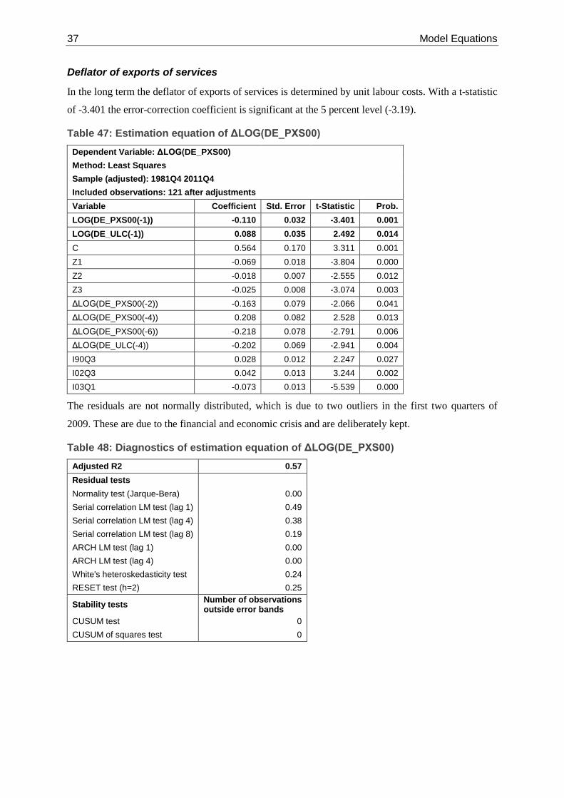
Deflator of exports of services

In the long term the deflator of exports of services is determined by unit labour costs. With a t-statistic

of -3.401 the error-correction coefficient is significant at the 5 percent level (-3.19).

Table 47: Estimation equation of ΔLOG(DE_PXS00) Dependent Variable: ΔLOG(DE_PXS00)



LOG(DE_PXS00(-1)) -0.110 0.032 -3.401 0.001 LOG(DE_ULC(-1)) 0.088 0.035 2.492 0.014 C 0.564 0.170 3.311 0.001 Z1 -0.069 0.018 -3.804 0.000 Z2 -0.018 0.007 -2.555 0.012 Z3 -0.025 0.008 -3.074 0.003 ΔLOG(DE_PXS00(-2)) -0.163 0.079 -2.066 0.041 ΔLOG(DE_PXS00(-4)) 0.208 0.082 2.528 0.013 ΔLOG(DE_PXS00(-6)) -0.218 0.078 -2.791 0.006 ΔLOG(DE_ULC(-4)) -0.202 0.069 -2.941 0.004 I90Q3 0.028 0.012 2.247 0.027 I02Q3 0.042 0.013 3.244 0.002 I03Q1 -0.073 0.013 -5.539 0.000

The residuals are not normally distributed, which is due to two outliers in the first two quarters of

2009. These are due to the financial and economic crisis and are deliberately kept.

Table 48: Diagnostics of estimation equation of ΔLOG(DE_PXS00) Adjusted R2 0.57 Residual tests Normality test (Jarque-Bera) 0.00 Serial correlation LM test (lag 1) 0.49 Serial correlation LM test (lag 4) 0.38 Serial correlation LM test (lag 8) 0.19 ARCH LM test (lag 1) 0.00 ARCH LM test (lag 4) 0.00 White's heteroskedasticity test 0.24 RESET test (h=2) 0.25



Model Equations 38

Deflator of imports of goods

An error-correction equation has been estimated for the deflator of imports of goods. In the long run

the latter is explained by the foreign price level in euro terms, the oil price in euro terms and a trend.

With a t-statistic of -3.309 the error-correction coefficient is not significant (5 percent critical value: -

3.91).

Table 49: Estimation equation of ΔLOG(DE_PMG00) Dependent Variable: ΔLOG(DE_PMG00)


LOG(DE_PMG00(-1)) -0.146 0.044 -3.309 0.001 LOG(DE_PTOTDEM(-1)/ DE_REEV_24_PTOTDEM(-1)) 0.050 0.030 1.700 0.092 LOG(OIL$(-1)/DE_NEV_US(-1)) 0.015 0.004 3.598 0.001 @TREND 0.000 0.000 -2.651 0.009 C 0.722 0.219 3.302 0.001 Z1 0.018 0.003 6.156 0.000 Z2 0.010 0.003 3.920 0.000 Z3 0.001 0.003 0.549 0.584 ΔLOG(DE_PMG00(-3)) 0.133 0.048 2.793 0.006 ΔLOG(DE_PTOTDEM/ DE_REEV_24_PTOTDEM) 0.568 0.065 8.692 0.000 ΔLOG(DE_PTOTDEM(-2)/ DE_REEV_24_PTOTDEM(-2)) 0.120 0.062 1.930 0.056 ΔLOG(OIL$/DE_NEV_US) 0.035 0.006 5.490 0.000 ΔLOG(OIL$(-1)/DE_NEV_US(-1)) 0.044 0.006 6.959 0.000 ΔLOG(OIL$(-2)/DE_NEV_US(-2)) -0.010 0.006 -1.549 0.125 ΔLOG(OIL$(-6)/DE_NEV_US(-6)) -0.010 0.006 -1.651 0.102 I95Q1 0.037 0.009 4.070 0.000

Except for White’s heteroskedasticity test the specification passes all diagnostic tests at the 5 percent

level.

Table 50: Diagnostics of estimation equation of ΔLOG(DE_PMG00) Adjusted R2 0.79 Residual tests Normality test (Jarque-Bera) 0.20 Serial correlation LM test (lag 1) 0.70 Serial correlation LM test (lag 4) 0.30 Serial correlation LM test (lag 8) 0.13 ARCH LM test (lag 1) 0.67 ARCH LM test (lag 4) 0.45 White's heteroskedasticity test 0.01 RESET test (h=2) 0.08



39 Model Equations

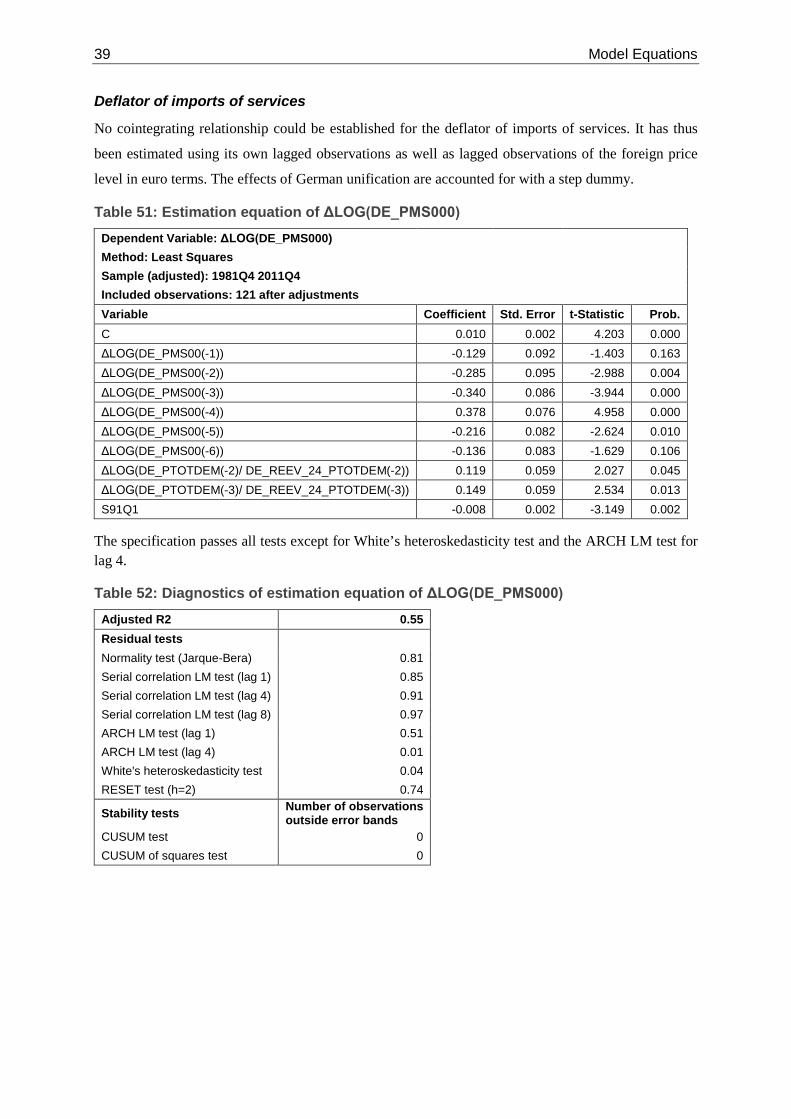
Deflator of imports of services

No cointegrating relationship could be established for the deflator of imports of services. It has thus

been estimated using its own lagged observations as well as lagged observations of the foreign price

level in euro terms. The effects of German unification are accounted for with a step dummy.

Table 51: Estimation equation of ΔLOG(DE_PMS000) Dependent Variable: ΔLOG(DE_PMS000)


C 0.010 0.002 4.203 0.000 ΔLOG(DE_PMS00(-1)) -0.129 0.092 -1.403 0.163 ΔLOG(DE_PMS00(-2)) -0.285 0.095 -2.988 0.004 ΔLOG(DE_PMS00(-3)) -0.340 0.086 -3.944 0.000 ΔLOG(DE_PMS00(-4)) 0.378 0.076 4.958 0.000 ΔLOG(DE_PMS00(-5)) -0.216 0.082 -2.624 0.010 ΔLOG(DE_PMS00(-6)) -0.136 0.083 -1.629 0.106 ΔLOG(DE_PTOTDEM(-2)/ DE_REEV_24_PTOTDEM(-2)) 0.119 0.059 2.027 0.045 ΔLOG(DE_PTOTDEM(-3)/ DE_REEV_24_PTOTDEM(-3)) 0.149 0.059 2.534 0.013 S91Q1 -0.008 0.002 -3.149 0.002

The specification passes all tests except for White’s heteroskedasticity test and the ARCH LM test for lag 4.

Table 52: Diagnostics of estimation equation of ΔLOG(DE_PMS000) Adjusted R2 0.55 Residual tests Normality test (Jarque-Bera) 0.81 Serial correlation LM test (lag 1) 0.85 Serial correlation LM test (lag 4) 0.91 Serial correlation LM test (lag 8) 0.97 ARCH LM test (lag 1) 0.51 ARCH LM test (lag 4) 0.01 White's heteroskedasticity test 0.04 RESET test (h=2) 0.74



Model Equations 40

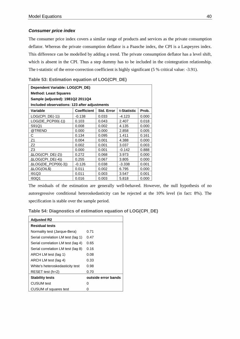
Consumer price index

The consumer price index covers a similar range of products and services as the private consumption

deflator. Whereas the private consumption deflator is a Paasche index, the CPI is a Laspeyres index.

This difference can be modelled by adding a trend. The private consumption deflator has a level shift,

which is absent in the CPI. Thus a step dummy has to be included in the cointegration relationship.

The t-statistic of the error-correction coefficient is highly significant (5 % critical value: -3.91).

Table 53: Estimation equation of LOG(CPI_DE) Dependent Variable: LOG(CPI_DE)



LOG(CPI_DE(-1)) -0.138 0.033 -4.123 0.000 LOG(DE_PCP00(-1)) 0.103 0.043 2.407 0.018 S91Q1 0.008 0.002 4.135 0.000 @TREND 0.000 0.000 2.858 0.005 C 0.134 0.095 1.411 0.161 Z1 0.004 0.001 4.388 0.000 Z2 0.002 0.001 3.037 0.003 Z3 0.000 0.001 -0.142 0.888 ΔLOG(CPI_DE(-2)) 0.272 0.068 3.973 0.000 ΔLOG(CPI_DE(-4)) 0.255 0.067 3.805 0.000 ΔLOG(DE_PCP00(-3)) -0.126 0.038 -3.338 0.001 ΔLOG(OIL$) 0.011 0.002 6.795 0.000 I91Q3 0.011 0.003 3.547 0.001 I93Q1 0.016 0.003 5.818 0.000

The residuals of the estimation are generally well-behaved. However, the null hypothesis of no

autoregressive conditional heteroskedasticity can be rejected at the 10% level (in fact: 8%). The

specification is stable over the sample period.

Table 54: Diagnostics of estimation equation of LOG(CPI_DE)

Adjusted R2 Residual tests Normality test (Jarque-Bera) 0.71

Serial correlation LM test (lag 1) 0.47 Serial correlation LM test (lag 4) 0.65 Serial correlation LM test (lag 8) 0.16 ARCH LM test (lag 1) 0.08 ARCH LM test (lag 4) 0.33 White's heteroskedasticity test 0.98 RESET test (h=2) 0.70 Stability tests outside error bands CUSUM test 0 CUSUM of squares test 0

41 Model Equations

3.1.3. Income and Employment

Consumption of fixed capital

There is a stable long-run relationship between consumption of fixed capital and the nominal capital stock calculated as the product of the real capital stock and the deflator of private non-residential capital formation. There are numerous outliers and the seasonal patterns change repeatedly.

Table 55: Estimation equation of LOG(DE_CFC) Dependent variable: DLOG(DE_CFC)

Method: Least squares Sample: 1983Q1 2011Q4 Included observations: 116 Variable Coefficient Std. Error t-Statistic Prob.

LOG(DE_CFC(-1)) -LOG(DE_CAPITAL00(-1)*DE_PIFC_ID(-1)/100) -0.012 0.002 -5.776 0.000 Z1 0.004 0.004 1.095 0.276 Z2 0.017 0.003 5.623 0.000 Z3 -0.014 0.004 -3.664 0.000 I91Q1 0.084 0.003 27.328 0.000 (1-S91Q1)*Z1 -0.023 0.003 -7.845 0.000 (1-S91Q1)*Z2 0.002 0.002 0.964 0.337 (1-S91Q1)*Z3 0.008 0.003 2.802 0.006 ΔLOG(DE_CFC(-2)) 0.081 0.031 2.569 0.012 ΔLOG(DE_CFC(-6)) 0.072 0.032 2.298 0.024 ΔLOG(DE_IFC(-1)) 0.033 0.008 4.007 0.000 ΔLOG(DE_IFC(-3)) 0.035 0.008 4.186 0.000 ΔLOG(DE_IFC(-4)) 0.018 0.009 2.059 0.042 ΔLOG(DE_IFC(-5)) 0.041 0.009 4.735 0.000 ΔLOG(DE_IFC(-6)) 0.032 0.009 3.626 0.001 S07Q1*Z1 0.014 0.002 6.452 0.000 S07Q1*Z2 0.005 0.002 2.368 0.020 S07Q1*Z3 0.006 0.002 2.665 0.009 I07Q1 0.013 0.003 4.015 0.000 I90Q1 0.020 0.003 6.266 0.000 I89Q1 0.014 0.003 4.655 0.000

The residuals can be assumed to be uncorrelated and homoskedastic. The specification is stable over the estimation period.

Table 56: Diagnostics of estimation equation of LOG(DE_CFC) Adjusted R2 0.95 Residual tests

Normality test (Jarque-Bera) 0.47 Serial correlation LM test (lag 1) 0.60 Serial correlation LM test (lag 4) 0.20 Serial correlation LM test (lag 8) 0.54 ARCH LM test (lag 1) 0.34 ARCH LM test (lag 4) 0.65 White's heteroskedasticity test 0.84 RESET test (h=2) 0.00 Stability tests Number of observations

outside error bands CUSUM test 0 CUSUM of squares test 0

Model Equations 42

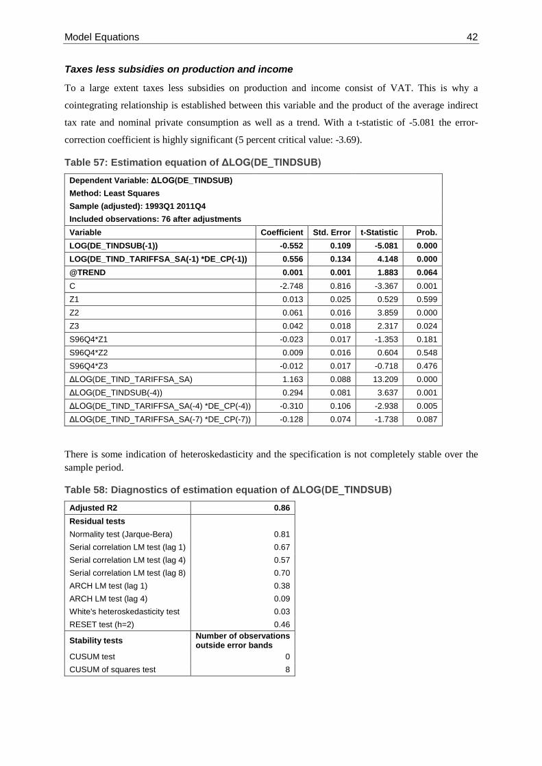
Taxes less subsidies on production and income

To a large extent taxes less subsidies on production and income consist of VAT. This is why a

cointegrating relationship is established between this variable and the product of the average indirect

tax rate and nominal private consumption as well as a trend. With a t-statistic of -5.081 the error-

correction coefficient is highly significant (5 percent critical value: -3.69).

Table 57: Estimation equation of ΔLOG(DE_TINDSUB) Dependent Variable: ΔLOG(DE_TINDSUB)


LOG(DE_TINDSUB(-1)) -0.552 0.109 -5.081 0.000 LOG(DE_TIND_TARIFFSA_SA(-1) *DE_CP(-1)) 0.556 0.134 4.148 0.000 @TREND 0.001 0.001 1.883 0.064 C -2.748 0.816 -3.367 0.001 Z1 0.013 0.025 0.529 0.599 Z2 0.061 0.016 3.859 0.000 Z3 0.042 0.018 2.317 0.024 S96Q4*Z1 -0.023 0.017 -1.353 0.181 S96Q4*Z2 0.009 0.016 0.604 0.548 S96Q4*Z3 -0.012 0.017 -0.718 0.476 ΔLOG(DE_TIND_TARIFFSA_SA) 1.163 0.088 13.209 0.000 ΔLOG(DE_TINDSUB(-4)) 0.294 0.081 3.637 0.001 ΔLOG(DE_TIND_TARIFFSA_SA(-4) *DE_CP(-4)) -0.310 0.106 -2.938 0.005 ΔLOG(DE_TIND_TARIFFSA_SA(-7) *DE_CP(-7)) -0.128 0.074 -1.738 0.087

There is some indication of heteroskedasticity and the specification is not completely stable over the sample period.

Table 58: Diagnostics of estimation equation of ΔLOG(DE_TINDSUB) Adjusted R2 0.86 Residual tests Normality test (Jarque-Bera) 0.81 Serial correlation LM test (lag 1) 0.67 Serial correlation LM test (lag 4) 0.57 Serial correlation LM test (lag 8) 0.70 ARCH LM test (lag 1) 0.38 ARCH LM test (lag 4) 0.09 White's heteroskedasticity test 0.03 RESET test (h=2) 0.46



43 Model Equations

Gross wage per employee

The main explaining variables are the GDP deflator (with a restricted coefficient), productivity and the

unemployment rate. As there are several structural breaks, which are partly due to German

reunification, some of the variables have been multiplied with step dummies. With a t-statistic of -

3.557 the error-correction coefficient is not significant. Nevertheless, the equation is being used as the

coefficients and elasticities seem sensible and there is no superior alternative.

Table 59: Estimation equation of ΔLOG(DE_GWAGEE) Dependent Variable: ΔLOG(DE_GWAGEE)


LOG(DE_GWAGEE(-1))-LOG(DE_PGDP00(-1)) -0.210 0.059 -3.557 0.001 LOG(DE_PRODEE(-1)) 0.137 0.046 2.960 0.004 DE_UR(-1)/100 -0.398 0.092 -4.311 0.000 S91Q1 0.723 0.305 2.369 0.020 LOG(DE_PRODEE(-1))*S91Q1 -0.074 0.032 -2.327 0.022 (DE_UR(-1)/100)*S94Q1 -0.205 0.040 -5.117 0.000 C -0.379 0.279 -1.358 0.178 Z1 -0.198 0.013 -15.314 0.000 Z2 -0.003 0.012 -0.270 0.788 Z3 -0.154 0.018 -8.505 0.000 ΔLOG(DE_GWAGEE(-2)) -0.498 0.060 -8.300 0.000 ΔLOG(DE_GWAGEE(-3)) -0.317 0.056 -5.664 0.000 ΔLOG(DE_GWAGEE(-6)) -0.171 0.034 -4.977 0.000 ΔLOG(DE_PGDP00(-1)) -0.782 0.146 -5.370 0.000 ΔLOG(DE_PRODEE(-1)) -0.246 0.044 -5.656 0.000 ΔLOG(DE_PRODEE(-3)) -0.143 0.045 -3.214 0.002 ΔLOG(DE_PRODEE(-5)) -0.098 0.029 -3.353 0.001 Δ(DE_UR(-2)/100) 0.622 0.277 2.242 0.027 I91Q1 -0.179 0.007 -23.910 0.000 I91Q1(-1) -0.073 0.012 -6.070 0.000 I91Q1(-2) -0.070 0.013 -5.258 0.000 I91Q1(-3) -0.061 0.013 -4.782 0.000 I84Q1 0.027 0.007 3.824 0.000 I84Q2 -0.042 0.007 -6.160 0.000 DUMMY_KA 0.000 0.000 -5.388 0.000

The RESET test points to some type of specification error, but otherwise the specification passes the

diagnostic tests.

Model Equations 44

Table 60: Diagnostics of estimation equation of ΔLOG(DE_GWAGEE)

Adjusted R2 Residual tests Normality test (Jarque-Bera) 0.83

Serial correlation LM test (lag 1) 0.46 Serial correlation LM test (lag 4) 0.14 Serial correlation LM test (lag 8) 0.27 ARCH LM test (lag 1) 0.75 ARCH LM test (lag 4) 0.24 White's heteroskedasticity test 0.09 RESET test (h=2) 0.00



Employees

In the long-run the number of employees is explained by the impact of the capital stock (adjusted for

technical progress using a modified trend) on productivity. A step dummy is included to account for

the level shift due to German reunification. With a t-statistic of -5.954 the error-correction coefficient

is highly significant (5 percent critical value: -3.69).

Table 61: Estimation equation of ΔLOG(DE_EE) Dependent Variable: ΔLOG(DE_EE)



LOG(DE_EE(-1))-LOG(DE_GDP00(-1)) -0.099 0.017 -5.954 0.000 LOG(DE_CAPITAL00(-1) +50*(100+(T80))) -0.065 0.011 -5.738 0.000 S91Q1 0.015 0.003 4.970 0.000 C 1.026 0.172 5.962 0.000 Z1 -0.009 0.003 -2.930 0.004 Z2 0.007 0.002 4.286 0.000 Z3 0.004 0.002 2.885 0.005 S91Q1*Z1 -0.001 0.002 -0.556 0.579 S91Q1*Z2 -0.004 0.002 -2.779 0.007 S91Q1*Z3 -0.004 0.002 -2.007 0.047 ΔLOG(DE_EE(-1)) +ΔLOG(DE_EE(-2)) 0.086 0.046 1.896 0.061 ΔLOG(DE_EE(-4)) 0.410 0.071 5.796 0.000 ΔLOG(DE_GDP00) 0.074 0.021 3.471 0.001 ΔLOG(DE_CAPITAL00(-1)) -0.255 0.106 -2.402 0.018 ΔLOG(DE_CAPITAL00(-2)) -0.236 0.101 -2.344 0.021 I90Q1 0.013 0.003 4.254 0.000 I91Q1 0.289 0.006 50.816 0.000 I91Q1(-4) -0.130 0.023 -5.559 0.000 DUMMY_KA(-4) 0.000 0.000 3.079 0.003

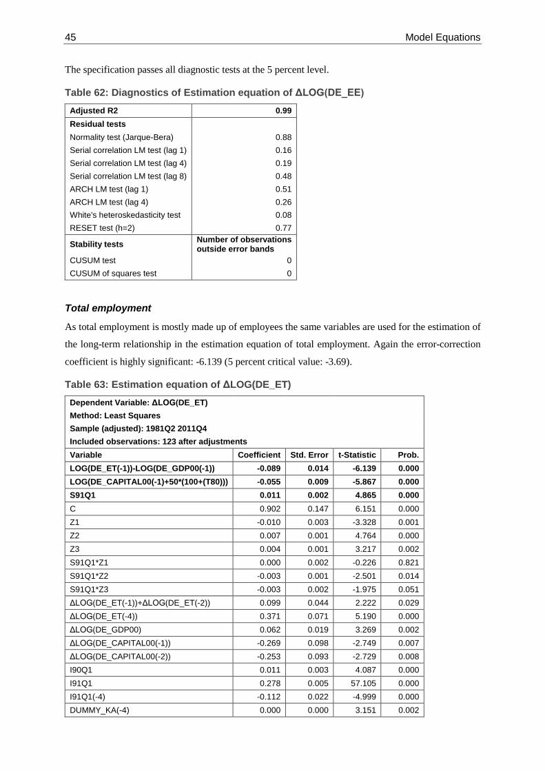
45 Model Equations


Table 62: Diagnostics of Estimation equation of ΔLOG(DE_EE) Adjusted R2 0.99 Residual tests Normality test (Jarque-Bera) 0.88 Serial correlation LM test (lag 1) 0.16 Serial correlation LM test (lag 4) 0.19 Serial correlation LM test (lag 8) 0.48 ARCH LM test (lag 1) 0.51 ARCH LM test (lag 4) 0.26 White's heteroskedasticity test 0.08 RESET test (h=2) 0.77



Total employment

As total employment is mostly made up of employees the same variables are used for the estimation of

the long-term relationship in the estimation equation of total employment. Again the error-correction

coefficient is highly significant: -6.139 (5 percent critical value: -3.69).

Table 63: Estimation equation of ΔLOG(DE_ET) Dependent Variable: ΔLOG(DE_ET)


Variable Coefficient Std. Error t-Statistic Prob. LOG(DE_ET(-1))-LOG(DE_GDP00(-1)) -0.089 0.014 -6.139 0.000 LOG(DE_CAPITAL00(-1)+50*(100+(T80))) -0.055 0.009 -5.867 0.000 S91Q1 0.011 0.002 4.865 0.000 C 0.902 0.147 6.151 0.000 Z1 -0.010 0.003 -3.328 0.001 Z2 0.007 0.001 4.764 0.000 Z3 0.004 0.001 3.217 0.002 S91Q1*Z1 0.000 0.002 -0.226 0.821 S91Q1*Z2 -0.003 0.001 -2.501 0.014 S91Q1*Z3 -0.003 0.002 -1.975 0.051 ΔLOG(DE_ET(-1))+ΔLOG(DE_ET(-2)) 0.099 0.044 2.222 0.029 ΔLOG(DE_ET(-4)) 0.371 0.071 5.190 0.000 ΔLOG(DE_GDP00) 0.062 0.019 3.269 0.002 ΔLOG(DE_CAPITAL00(-1)) -0.269 0.098 -2.749 0.007 ΔLOG(DE_CAPITAL00(-2)) -0.253 0.093 -2.729 0.008 I90Q1 0.011 0.003 4.087 0.000 I91Q1 0.278 0.005 57.105 0.000 I91Q1(-4) -0.112 0.022 -4.999 0.000 DUMMY_KA(-4) 0.000 0.000 3.151 0.002

Model Equations 46


Table 64: Diagnostics of estimation equation of ΔLOG(DE_ET) Adjusted R2 0.99 Residual tests Normality test (Jarque-Bera) 0.69 Serial correlation LM test (lag 1) 0.32 Serial correlation LM test (lag 4) 0.31 Serial correlation LM test (lag 8) 0.63 ARCH LM test (lag 1) 0.44 ARCH LM test (lag 4) 0.53 White's heteroskedasticity test 0.28 RESET test (h=2) 0.77 Stability tests outside error bands CUSUM test 0 CUSUM of squares test 0

Unemployment

There is an inverse long-term relationship between employment and unemployment. Some structural

changes are accounted for by step dummies. With a t-statistic of -6.717 the error-correction coefficient

is highly significant (5 percent critical value: -3.74).

Table 65: Estimation equation of Δ(DE_U) Dependent Variable: Δ(DE_U)



DE_U(-1) -0.088 0.013 -6.717 0.000 DE_EE(-1) -0.027 0.006 -4.230 0.000 S91Q1 452.583 68.480 6.609 0.000 S06Q1 -58.329 20.802 -2.804 0.006 C 832.453 149.439 5.571 0.000 Z1 146.905 48.855 3.007 0.003 Z2 -408.881 40.875 -10.003 0.000 Z3 -10.883 35.002 -0.311 0.757 Z1*S91Q1 324.004 49.216 6.583 0.000 Z2*S91Q1 82.828 38.917 2.128 0.036 Z3*S91Q1 140.700 42.365 3.321 0.001 Δ(DE_U(-1)) 0.413 0.070 5.874 0.000 Δ(DE_EE(-1)) -0.018 0.007 -2.458 0.016 ΔLOG(DE_GDP00(-4)) -1157.427 363.500 -3.184 0.002 I05Q1 555.800 69.305 8.020 0.000 I05Q2 -213.482 80.722 -2.645 0.009

The CUSUM of squares test indicates some instability. Otherwise the specification passes all

diagnostic tests at the 5 percent level.

47 Model Equations

Table 66: Diagnostics of estimation equation of Δ(DE_U) Adjusted R2 0.94 Residual tests Normality test (Jarque-Bera) 0.24 Serial correlation LM test (lag 1) 0.17 Serial correlation LM test (lag 4) 0.18 Serial correlation LM test (lag 8) 0.26 ARCH LM test (lag 1) 0.18 ARCH LM test (lag 4) 0.75 White's heteroskedasticity test 0.09 RESET test (h=2) 0.87



Distributed profits

In the long term distributed profits are explained by operating surplus and mixed income less direct

taxes on operating surplus and mixed income and a trend beginning in 1970. Although the error-

correction coefficient is not significant this specification is adhered to because it makes economic

sense and there is no viable alternative.

Table 67: Estimation equation of ΔLOG(DE_WDYENT) Dependent Variable: ΔLOG(DE_WDYENT)


LOG(DE_WDYENT(-1)) -0.302 0.104 -2.917 0.005 LOG(DE_GYPROP(-1)-DE_TDIREM1(-1)) 0.139 0.066 2.129 0.037 @TREND(1970:1) 0.001 0.001 2.061 0.043 C 0.541 0.307 1.761 0.083 Z1 0.005 0.042 0.121 0.904 Z2 0.066 0.030 2.228 0.029 Z3 -0.017 0.036 -0.484 0.630 ΔLOG(DE_GYPROP-DE_TDIREM1) 0.380 0.068 5.569 0.000 ΔLOG(DE_GYPROP(-2)-DE_TDIREM1(-2)) +ΔLOG(DE_GYPROP(-3)-DE_TDIREM1(-3)) 0.112 0.054 2.096 0.040

ΔLOG(DE_WDYENT(-1)) -0.149 0.093 -1.608 0.113 ΔLOG(DE_WDYENT(-2)) -0.212 0.087 -2.448 0.017

ΔLOG(DE_WDYENT(-4)-DE_RES_WDYENT(-4)) 0.382 0.075 5.085 0.000

The residuals are well-behaved. There may be some heteroskedasticity in the residuals. The specification is stable over the sample period.

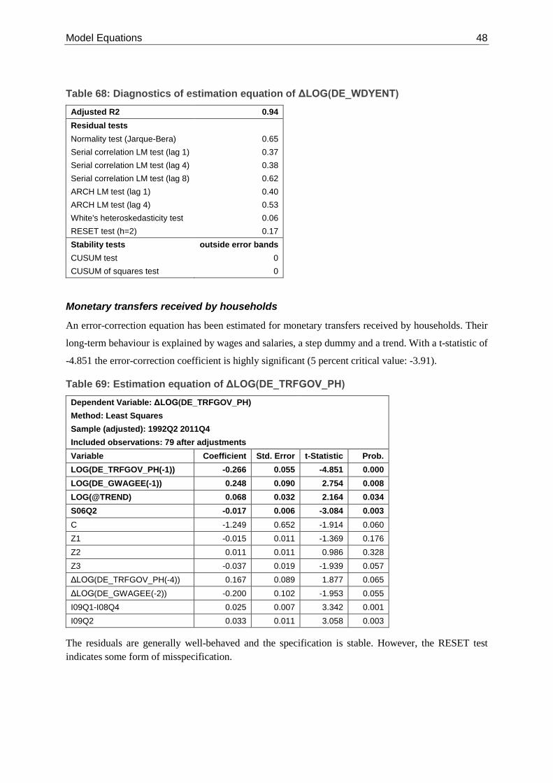
Model Equations 48

Table 68: Diagnostics of estimation equation of ΔLOG(DE_WDYENT) Adjusted R2 0.94 Residual tests Normality test (Jarque-Bera) 0.65 Serial correlation LM test (lag 1) 0.37 Serial correlation LM test (lag 4) 0.38 Serial correlation LM test (lag 8) 0.62 ARCH LM test (lag 1) 0.40 ARCH LM test (lag 4) 0.53 White's heteroskedasticity test 0.06 RESET test (h=2) 0.17 Stability tests outside error bands CUSUM test 0 CUSUM of squares test 0

Monetary transfers received by households

An error-correction equation has been estimated for monetary transfers received by households. Their

long-term behaviour is explained by wages and salaries, a step dummy and a trend. With a t-statistic of

-4.851 the error-correction coefficient is highly significant (5 percent critical value: -3.91).

Table 69: Estimation equation of ΔLOG(DE_TRFGOV_PH) Dependent Variable: ΔLOG(DE_TRFGOV_PH)



LOG(DE_TRFGOV_PH(-1)) -0.266 0.055 -4.851 0.000 LOG(DE_GWAGEE(-1)) 0.248 0.090 2.754 0.008 LOG(@TREND) 0.068 0.032 2.164 0.034 S06Q2 -0.017 0.006 -3.084 0.003 C -1.249 0.652 -1.914 0.060 Z1 -0.015 0.011 -1.369 0.176 Z2 0.011 0.011 0.986 0.328 Z3 -0.037 0.019 -1.939 0.057 ΔLOG(DE_TRFGOV_PH(-4)) 0.167 0.089 1.877 0.065 ΔLOG(DE_GWAGEE(-2)) -0.200 0.102 -1.953 0.055 I09Q1-I08Q4 0.025 0.007 3.342 0.001 I09Q2 0.033 0.011 3.058 0.003

The residuals are generally well-behaved and the specification is stable. However, the RESET test indicates some form of misspecification.

49 Model Equations

Table 70: Diagnostics of estimation equation of ΔLOG(DE_TRFGOV_PH) Adjusted R2 0.77 Residual tests Normality test (Jarque-Bera) 0.84 Serial correlation LM test (lag 1) 0.66 Serial correlation LM test (lag 4) 0.35 Serial correlation LM test (lag 8) 0.52 ARCH LM test (lag 1) 0.48 ARCH LM test (lag 4) 0.39 White's heteroskedasticity test 0.24 RESET test (h=2) 0.00 Stability tests outside error bands CUSUM test 0 CUSUM of squares test 0

Model Equations 50

3.1.4. General Government

3.1.4.1. Expenditures

Unlike the other government expenditure aggregates nominal government expenditure is not estimated

directly. Instead it is calculated as the product of real government consumption and the government

consumption deflator divided by 100. Definitions are presented in section 3.2.5. All other government

expenditures are estimated. The equations are presented below.

Monetary transfers

Like monetary transfers received by households monetary transfers paid by the government move in

line with wages and salaries in the long run. The error-correction coefficient is significant exhibiting a

t-statistic of -3.569 (5 percent critical value: -3.41). Unemployment plays a role only for the short-term

dynamics.

Table 71: Estimation equation of ΔLOG(DE_TRFGOV) Dependent Variable: ΔLOG(DE_TRFGOV)



LOG(DE_TRFGOV(-1)) -0.093 0.026 -3.569 0.001 LOG(DE_GWAGEE(-5)) 0.088 0.044 2.006 0.049 C -0.343 0.280 -1.225 0.225 Z1 -0.067 0.016 -4.037 0.000 Z2 0.035 0.018 1.951 0.055 Z3 -0.043 0.014 -3.002 0.004 ΔLOG(DE_U) 0.176 0.044 4.012 0.000 ΔLOG(DE_TRFGOV(-1))+ΔLOG(DE_TRFGOV(-2)) -0.171 0.064 -2.673 0.009 ΔLOG(DE_GWAGEE(-1)) 0.388 0.095 4.096 0.000 ΔLOG(DE_GWAGEE(-3)) 0.210 0.049 4.316 0.000 I09Q2 0.031 0.011 2.886 0.005

The specification passes all diagnostic tests. The residuals are well-behaved and the estimation

equation is stable over the sample period.

51 Model Equations

Table 72: Diagnostics of estimation equation of ΔLOG(DE_TRFGOV) Adjusted R2 0.86 Residual tests Normality test (Jarque-Bera) 0.79 Serial correlation LM test (lag 1) 0.81 Serial correlation LM test (lag 4) 0.78 Serial correlation LM test (lag 8) 0.65 ARCH LM test (lag 1) 0.91 ARCH LM test (lag 4) 0.77 White's heteroskedasticity test 0.66 RESET test (h=2) 0.10 Stability tests outside error bands CUSUM test 0 CUSUM of squares test 0

Property income paid

Property income paid comprises the government’s interest payments on debt. A cointegrating

relationship has been established between property income paid and the product of government debt

and the long-term interest rate divided by 100. With a t-statistic of -6.200 the error-correction

coefficient is highly significant (5 percent critical value: -3.19).

Table 73: Estimation equation of ΔLOG(DE_INTPAGOV) Dependent Variable: ΔLOG(DE_INTPAGOV)


LOG(DE_INTPAGOV(-1)) -0.194 0.031 -6.200 0.000 LOG(DE_DBTGOV(-1)*DE_RL10Y(-1)/100) 0.058 0.026 2.191 0.032 C 0.305 0.099 3.082 0.003 Z1 -0.014 0.008 -1.797 0.076 Z2 0.006 0.008 0.827 0.411 Z3 -0.009 0.008 -1.145 0.256 ΔLOG(DE_INTPAGOV(-1)) -0.170 0.094 -1.817 0.073 I11Q1 0.092 0.025 3.662 0.001

Except for White’s heteroskedasticity test the specification passes all diagnostic tests.

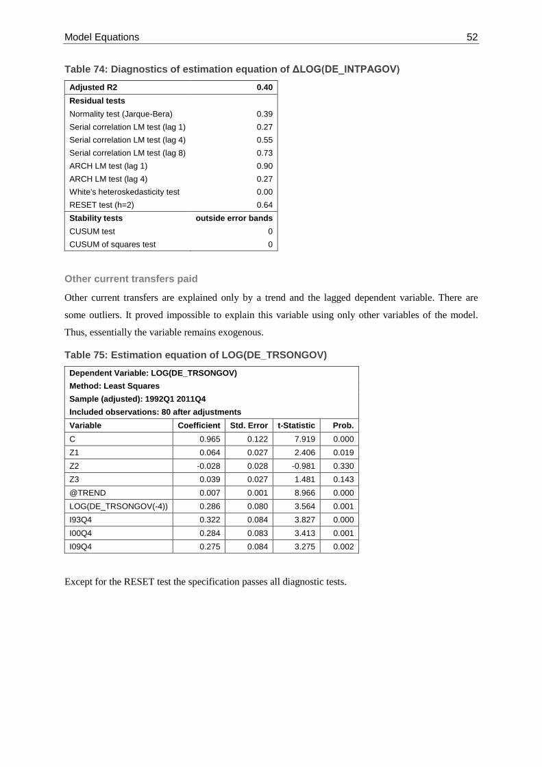
Model Equations 52

Table 74: Diagnostics of estimation equation of ΔLOG(DE_INTPAGOV) Adjusted R2 0.40 Residual tests Normality test (Jarque-Bera) 0.39 Serial correlation LM test (lag 1) 0.27 Serial correlation LM test (lag 4) 0.55 Serial correlation LM test (lag 8) 0.73 ARCH LM test (lag 1) 0.90 ARCH LM test (lag 4) 0.27 White's heteroskedasticity test 0.00 RESET test (h=2) 0.64 Stability tests outside error bands CUSUM test 0 CUSUM of squares test 0

Other current transfers paid

Other current transfers are explained only by a trend and the lagged dependent variable. There are

some outliers. It proved impossible to explain this variable using only other variables of the model.

Thus, essentially the variable remains exogenous.

Table 75: Estimation equation of LOG(DE_TRSONGOV) Dependent Variable: LOG(DE_TRSONGOV)



C 0.965 0.122 7.919 0.000 Z1 0.064 0.027 2.406 0.019 Z2 -0.028 0.028 -0.981 0.330 Z3 0.039 0.027 1.481 0.143 @TREND 0.007 0.001 8.966 0.000 LOG(DE_TRSONGOV(-4)) 0.286 0.080 3.564 0.001 I93Q4 0.322 0.084 3.827 0.000 I00Q4 0.284 0.083 3.413 0.001 I09Q4 0.275 0.084 3.275 0.002

Except for the RESET test the specification passes all diagnostic tests.

53 Model Equations

Table 76: Diagnostics of estimation equation of LOG(DE_TRSONGOV) Adjusted R2 0.89 Residual tests Normality test (Jarque-Bera) 0.52 Serial correlation LM test (lag 1) 0.10 Serial correlation LM test (lag 4) 0.18 Serial correlation LM test (lag 8) 0.16 ARCH LM test (lag 1) 0.40 ARCH LM test (lag 4) 0.46 White's heteroskedasticity test 0.60 RESET test (h=2) 0.01 Stability tests outside error bands CUSUM test 0 CUSUM of squares test 0

Capital transfers paid

This variable is I(0). Therefore no attempts were made to estimate an error-correction equation. In

addition the variable seems totally uncorrelated with any other model variable. It is thus explained

only by lagged observations and deterministics.

Table 77: Estimation equation of LOG(DE_PROTRGOV) Dependent Variable: LOG(DE_PROTRGOV)



C 2.017 0.163 12.397 0.000 Z1 -0.163 0.075 -2.179 0.033 Z2 -0.527 0.088 -5.998 0.000 Z3 -0.496 0.081 -6.095 0.000 @TREND 0.004 0.001 3.203 0.002 LOG(DE_PROTRGOV(-2)) -0.200 0.078 -2.564 0.012 I95Q1 2.671 0.237 11.283 0.000 I95Q3 1.919 0.316 6.077 0.000 I10Q3 1.734 0.239 7.259 0.000

Due to the limited availability of suitable variables it has proved impossible to estimate an equation

that passes all diagnostic tests. Auto-correlation and heteroskedasticity could not be avoided.

Model Equations 54

Table 78: Diagnostics of estimation equation of LOG(DE_PROTRGOV) Adjusted R2 0.81 Residual tests Normality test (Jarque-Bera) 0.43 Serial correlation LM test (lag 1) 0.70 Serial correlation LM test (lag 4) 0.00 Serial correlation LM test (lag 8) 0.00 ARCH LM test (lag 1) 0.14 ARCH LM test (lag 4) 0.00 White's heteroskedasticity test 0.00 RESET test (h=2) 0.55 Stability tests outside error bands CUSUM test 0 CUSUM of squares test 7

Net acquisition of non-produced assets

This variable is I(0). Therefore no attempts were made to estimate an error-correction equation. In

addition the variable seems totally uncorrelated with any other model variable. It is thus explained

only by lagged observations and deterministics.

Table 79: Estimation equation of DE_NETPRGOV Dependent Variable: DE_NETPRGOV



C -0.364 0.009 -41.627 0.000 Z1 0.145 0.022 6.574 0.000 Z2 0.149 0.022 6.749 0.000 Z3 0.104 0.022 4.740 0.000 (1-S95Q1)*@TREND 0.001 0.000 3.461 0.001 DE_NETPRGOV(-1) -0.002 0.001 -1.233 0.222 I00Q3 -50.773 0.072 -709.156 0.000 I10Q2 -4.359 0.072 -60.892 0.000

Except for the RESET test the estimation equation passes all specification tests. The residuals are

uncorrelated and can be assumed to be homoskedastic. The specification is stable over the sample

period.

55 Model Equations

Table 80: Diagnostics of estimation equation of DE_NETPRGOV Adjusted R2 0.9999 Residual tests Normality test (Jarque-Bera) 0.12 Serial correlation LM test (lag 1) 0.12 Serial correlation LM test (lag 4) 0.17 Serial correlation LM test (lag 8) 0.52 ARCH LM test (lag 1) 0.96 ARCH LM test (lag 4) 0.22 White's heteroskedasticity test 0.28 RESET test (h=2) 0.03 Stability tests outside error bands CUSUM test 0 CUSUM of squares test 0

Other expenditures

Other expenditures are also explained by past observations and deterministics.

Table 81: Estimation equation of LOG(DE_EXPOTH) Dependent Variable: LOG(DE_EXPOTH)



C 0.230 0.099 2.314 0.024 Z1 -0.319 0.049 -6.554 0.000 Z2 -0.237 0.045 -5.315 0.000 Z3 -0.070 0.045 -1.551 0.126 LOG(DE_EXPOTH(-1)) 0.384 0.087 4.411 0.000 LOG(DE_EXPOTH(-3)) 0.111 0.050 2.196 0.032 LOG(DE_EXPOTH(-4)) 0.122 0.051 2.381 0.021 LOG(DE_EXPOTH(-7)) 0.104 0.050 2.079 0.042 LOG(DE_EXPOTH(-8)) 0.105 0.051 2.067 0.043 I95Q1 0.623 0.087 7.153 0.000 I95Q2 -1.550 0.099 -15.624 0.000 I95Q3 0.418 0.143 2.932 0.005 I00Q3 -0.395 0.088 -4.510 0.000 I00Q4 0.478 0.093 5.147 0.000 S05Q1 0.144 0.045 3.155 0.003 I11Q1 0.198 0.093 2.127 0.038

There is some indication of higher order autocorrelation. The specification is stable and the residuals

are homoskedastic.

Model Equations 56

Table 82: Diagnostics of estimation equation of LOG(DE_EXPOTH) Adjusted R2 0.96 Residual tests Normality test (Jarque-Bera) 0.61 Serial correlation LM test (lag 1) 0.76 Serial correlation LM test (lag 4) 0.00 Serial correlation LM test (lag 8) 0.00 ARCH LM test (lag 1) 0.89 ARCH LM test (lag 4) 0.89 White's heteroskedasticity test 0.79 RESET test (h=2) 0.08 Stability tests outside error bands CUSUM test 0 CUSUM of squares test 0

3.1.4.2. Revenues

Social contributions from employees and from employers are calculated from gross wages and salaries

and the seasonally adjusted average contribution rates (for the documentation of the definition see

section 3.2.5 below).

Indirect taxes

Most indirect taxes are closely connected to nominal private consumption. This is why a cointegrating

relationship has been established between indirect taxes and nominal private consumption multiplied

by the average seasonally adjusted indirect tax rate. With a t-statistic of -3.785 the error-correction

coefficient is significant (5 percent critical value: -3.41).

Table 83: Estimation equation of ΔLOG(DE_TIND) Dependent Variable: ΔLOG(DE_TIND)


LOG(DE_TIND(-1)) -0.670 0.177 -3.785 0.000 LOG(DE_TIND_TARIFFSA_SA(-1) *DE_CP00(-1)*DE_PCP00(-1)/100) 0.652 0.178 3.667 0.001

C -2.919 0.823 -3.547 0.001 Z1 -0.036 0.009 -3.794 0.000 Z2 -0.031 0.011 -2.725 0.008 Z3 -0.045 0.007 -6.094 0.000 S96Q4*Z1 0.006 0.010 0.575 0.567 S96Q4*Z2 0.040 0.009 4.555 0.000 S96Q4*Z3 0.043 0.008 5.134 0.000 ΔLOG(DE_TIND_TARIFFSA_SA) 1.005 0.056 17.822 0.000 ΔLOG(DE_TIND(-1)) -0.445 0.096 -4.638 0.000 ΔLOG(DE_TIND_TARIFFSA_SA(-1)) 0.469 0.108 4.353 0.000 I08Q4 -0.026 0.012 -2.109 0.039

57 Model Equations

The residuals show some higher-order autocorrelation as well as heteroskedasticity. Further the

specification is not completely stable over the sample.

Table 84: Diagnostics of estimation equation of ΔLOG(DE_TIND) Adjusted R2 0.89 Residual tests Normality test (Jarque-Bera) 0.76 Serial correlation LM test (lag 1) 0.45 Serial correlation LM test (lag 4) 0.03 Serial correlation LM test (lag 8) 0.06 ARCH LM test (lag 1) 0.93 ARCH LM test (lag 4) 0.15 White's heteroskedasticity test 0.05 RESET test (h=2) 0.38 Stability tests outside error bands CUSUM test 0 CUSUM of squares test 7

Direct taxes on wages and salaries

The long-term evolution of direct taxes on wages and salaries is explained by gross wages and salaries

per employee, the number of employees and a step dummy accounting for tax reform at the turn of the

millennium.

Table 85: Estimation equation of ΔLOG(DE_TDIREE) Dependent Variable: ΔLOG(DE_TDIREE)


LOG(DE_TDIREE(-1)) -0.273 0.056 -4.889 0.000 LOG(DE_GWAGEE(-1)) 0.353 0.077 4.589 0.000 LOG(DE_EE(-1)) 0.221 0.064 3.462 0.001 S00Q1 -0.029 0.008 -3.458 0.001 C -4.392 0.973 -4.516 0.000 Z1 -0.083 0.043 -1.906 0.060 Z2 -0.087 0.039 -2.231 0.028 Z3 -0.130 0.044 -2.928 0.004 ΔLOG(DE_TDIREE(-1)) 0.213 0.085 2.515 0.013 ΔLOG(DE_TDIREE(-3)) -0.182 0.059 -3.069 0.003 ΔLOG(DE_TDIREE(-4)) 0.625 0.057 11.013 0.000 ΔLOG(DE_EE(-1)) -0.301 0.157 -1.916 0.058 ΔLOG(DE_GWAGEE(-1)) -0.915 0.249 -3.672 0.000 ΔLOG(DE_GWAGEE(-2)) -0.517 0.122 -4.229 0.000 I90Q1 -0.116 0.026 -4.563 0.000

Except for White’s heteroskedasticity test the specification passes all diagnostic tests.

Model Equations 58

Table 86: Diagnostics of estimation equation of ΔLOG(DE_TDIREE) Adjusted R2 0.99 Residual tests Normality test (Jarque-Bera) 0.53 Serial correlation LM test (lag 1) 0.29 Serial correlation LM test (lag 4) 0.82 Serial correlation LM test (lag 8) 0.93 ARCH LM test (lag 1) 0.52 ARCH LM test (lag 4) 0.47 White's heteroskedasticity test 0.01 RESET test (h=2) 0.38 Stability tests outside error bands CUSUM test 0 CUSUM of squares test 0

Direct taxes on operating surplus and mixed income

In the long term direct taxes on operating surplus and mixed income depend on operating surplus and

mixed income. With a t-statistic of -4.071 the error-correction coefficient is highly significant

(5 percent critical value: -3.69).

Table 87: Estimation equation of ΔLOG(DE_TDIREM1)

Dependent Variable: ΔLOG(DE_TDIREM1) Method: Least Squares

Sample (adjusted): 1992Q4 2011Q4 Included observations: 77 after adjustments

Variable Coefficient Std. Error t-Statistic Prob. LOG(DE_TDIREM1(-1)) -0.151 0.037 -4.071 0.000 LOG(DE_GYPROP(-1)) 0.165 0.045 3.689 0.001 C -0.315 0.144 -2.194 0.032 Z1 -0.040 0.042 -0.944 0.349 Z2 -0.021 0.019 -1.109 0.272 Z3 -0.118 0.057 -2.092 0.041 ΔLOG(DE_TDIREM1(-1)) 0.694 0.094 7.353 0.000 ΔLOG(DE_TDIREM1(-2)) -0.344 0.093 -3.686 0.001 ΔLOG(DE_TDIREM1(-4)) 0.790 0.093 8.507 0.000 ΔLOG(DE_TDIREM1(-5)) -0.446 0.110 -4.051 0.000 ΔLOG(DE_TDIREM1(-6)) 0.340 0.109 3.132 0.003 ΔLOG(DE_GYPROP(-7)) -0.205 0.105 -1.946 0.056 Δ (DE_RS3M(-3)) -0.043 0.013 -3.283 0.002 I95Q1 -0.124 0.041 -2.996 0.004

The residuals are well-behaved and the specification is stable over the sample. All diagnostic tests are

passed.

59 Model Equations

Table 88: Diagnostics of estimation equation of ΔLOG(DE_TDIREM1) Adjusted R2 0.88 Residual tests

Normality test (Jarque-Bera) 0.16


Serial correlation LM test (lag 4) 0.99 Serial correlation LM test (lag 8) 0.29 ARCH LM test (lag 1) 0.97 ARCH LM test (lag 4) 0.91 White's heteroskedasticity test 0.91 RESET test (h=2) 0.41 Stability tests outside error bands CUSUM test 0 CUSUM of squares test 0

Property income received

Property income receive is also estimated as an error-correction equation. There is a long-run

relationship between property income received, the nominal short-term interest rate and a linear trend.

The error-correction coefficient is highly significant exhibiting a t-statistic of -5.175 compared to the 5

percent critical value of -3.69.

Table 89: Estimation equation of ΔLOG(DE_YPROGOV) Dependent Variable: ΔLOG(DE_YPROGOV)



LOG(DE_YPROGOV(-1)) -0.489 0.094 -5.175 0.000 @TREND 0.003 0.001 3.076 0.003 DE_RS3M(-1) 0.031 0.012 2.583 0.012 C 0.330 0.149 2.217 0.030 Z1 -0.043 0.093 -0.461 0.646 Z2 1.109 0.083 13.429 0.000 Z3 -0.065 0.139 -0.468 0.642 Z1*S05Q1 0.649 0.111 5.839 0.000 Z2*S05Q1 -0.982 0.108 -9.069 0.000 Z3*S05Q1 -0.064 0.164 -0.391 0.697 ΔLOG(DE_YPROGOV(-1)) -0.245 0.083 -2.941 0.004 I04Q2 -1.013 0.149 -6.817 0.000 I05Q1 -0.681 0.153 -4.456 0.000

The CUSUM of squares test indicates some instability. Otherwise the specification passes all

diagnostic tests.

Model Equations 60

Table 90: Diagnostics of estimation equation of ΔLOG(DE_YPROGOV)

Adjusted R2 0.95 Residual tests Normality test (Jarque-Bera) 0.21 Serial correlation LM test (lag 1) 0.35 Serial correlation LM test (lag 4) 0.23 Serial correlation LM test (lag 8) 0.11 ARCH LM test (lag 1) 0.87 ARCH LM test (lag 4) 0.23 White's heteroskedasticity test 0.80 RESET test (h=2) 0.13 Stability tests outside error bands CUSUM test 0 CUSUM of squares test 11

Other current transfers received

Other current transfers received cannot be explained by any other variable of the model. Rather the

variable is estimated using lagged observations and deterministics. There are also numerous outliers.

In fact, the variable remains exogenous.

Table 91: Estimation equation of DE_REVYTRF Dependent Variable: DE_REVYTRF



C 1.243 0.291 4.272 0.000 Z1 -0.600 0.094 -6.374 0.000 Z2 -0.485 0.087 -5.562 0.000 Z3 -0.275 0.088 -3.131 0.003 @TREND 0.004 0.001 2.451 0.017 DE_REVYTRF(-1) 0.586 0.089 6.616 0.000 I92Q3 0.661 0.286 2.315 0.024 I04Q4 1.748 0.287 6.098 0.000 I05Q1 2.010 0.340 5.909 0.000 I05Q2 -1.738 0.408 -4.258 0.000 I09Q1 -0.468 0.287 -1.633 0.107

The serial correlation LM test indicates higher-order autocorrelation and the specification is not

completely stable over the sample.

61 Model Equations

Table 92: Diagnostics of estimation equation of DE_REVYTRF Adjusted R2 0.81 Residual tests Normality test (Jarque-Bera) 0.44 Serial correlation LM test (lag 1) 0.72 Serial correlation LM test (lag 4) 0.02 Serial correlation LM test (lag 8) 0.04 ARCH LM test (lag 1) 0.74 ARCH LM test (lag 4) 0.67 White's heteroskedasticity test 0.78 RESET test (h=2) 0.99 Stability tests outside error bands CUSUM test 0 CUSUM of squares test 4

Capital transfers received

Being I(0) capital transfers received are estimated in log-levels. Explaining variables are limited to the

lagged dependent variable and deterministics. The specification passes all diagnostic tests except for

the RESET test.

Table 93: Estimation equation of LOG(DE_RECPROTR) Dependent Variable: LOG(DE_RECPROTR)



C -1.301 0.298 -4.371 0.000 Z1 -0.069 0.042 -1.629 0.108 Z2 -0.176 0.046 -3.853 0.000 Z3 -0.116 0.043 -2.673 0.009 LOG(@TREND) 0.422 0.076 5.562 0.000 I95Q1 0.939 0.136 6.897 0.000 LOG(DE_RECPROTR(-4)) 0.226 0.084 2.686 0.009

Table 94: Diagnostics of estimation equation of LOG(DE_RECPROTR) Adjusted R2 0.70 Residual tests Normality test (Jarque-Bera) 0.40 Serial correlation LM test (lag 1) 0.67 Serial correlation LM test (lag 4) 0.98 Serial correlation LM test (lag 8) 0.66 ARCH LM test (lag 1) 0.66 ARCH LM test (lag 4) 0.29 White's heteroskedasticity test 0.28 RESET test (h=2) 0.00 Stability tests outside error bands CUSUM test 0 CUSUM of squares test 0

Model Equations 62

Sales and other subsidies

cannot be explained by any other variable of the model. Rather the variable is estimated using lagged

observations and deterministics. Thus, in fact, the variable remains exogenous.

Table 95: Estimation equation of DE_SALESSUB Dependent Variable: DE_SALESSUB



C -0.172 0.180 -0.958 0.342 Z1 -1.096 0.330 -3.319 0.001 Z2 -0.007 0.164 -0.045 0.964 Z3 -0.086 0.313 -0.274 0.785 DE_SALESSUB(-1) 0.899 0.066 13.631 0.000 DE_SALESSUB(-3) -0.155 0.081 -1.909 0.060 DE_SALESSUB(-4) 0.790 0.090 8.821 0.000 DE_SALESSUB(-5) -0.512 0.083 -6.192 0.000 I04Q2 -0.659 0.235 -2.808 0.007 I11Q1 0.699 0.242 2.889 0.005

The CUSUM of squares test points to some instability. Otherwise the specification passes all

diagnostic tests.

Table 96: Diagnostics of estimation equation of DE_SALESSUB Adjusted R2 0.99 Residual tests Normality test (Jarque-Bera) 0.99 Serial correlation LM test (lag 1) 0.86 Serial correlation LM test (lag 4) 0.53 Serial correlation LM test (lag 8) 0.39 ARCH LM test (lag 1) 0.99 ARCH LM test (lag 4) 0.63 White's heteroskedasticity test 0.45 RESET test (h=2) 0.66 Stability tests outside error bands CUSUM test 0 CUSUM of squares test 2

63 Model Equations

3.1.5. Other variables

Nominal changes in inventories and net acquisitions of valuables

The variable is I(0). Therefore an error-correction equation is not appropriate. Changes in inventories

and net acquisitions of valuables are explained by past observations, the coincident change of total

demand and deterministics.

Table 97: Estimation equation of DE_INV Dependent Variable: DE_INV



C -0.158 0.299 -0.527 0.599 Z1 14.892 2.089 7.129 0.000 Z2 3.997 1.270 3.147 0.002 Z3 10.404 1.612 6.454 0.000 DE_INV(-1) 0.281 0.073 3.845 0.000 DE_INV(-4) 0.511 0.071 7.158 0.000 S91Q1*Z1 6.859 1.653 4.149 0.000 S91Q1*Z2 -2.182 1.511 -1.444 0.152 S91Q1*Z3 3.067 1.657 1.851 0.067 Δ(DE_GDP+DE_M) 0.066 0.025 2.641 0.010 I06Q4 -9.938 2.671 -3.720 0.000 I09Q2 -11.760 2.712 -4.336 0.000 I09Q2(2) 3.756 2.849 1.318 0.190

Except for White’s heteroskedasticity test the specification passes all diagnostic tests at the 5 percent

level. However, the probability of first order autocorrelation is close to 5 percent.

Table 98: Diagnostics of estimation equation of DE_INV Adjusted R2 0.94 Residual tests Normality test (Jarque-Bera) 0.67 Serial correlation LM test (lag 1) 0.06 Serial correlation LM test (lag 4) 0.18 Serial correlation LM test (lag 8) 0.20 ARCH LM test (lag 1) 0.72 ARCH LM test (lag 4) 0.52 White's heteroskedasticity test 0.00 RESET test (h=2) 0.06 Stability tests outside error bands CUSUM test 0 CUSUM of squares test 65

Model Equations 64

3.2. Definitions

3.2.1. Real GDP

de_gdp00 = (1 - s91q1agg) * (de_cp00 + de_cgov00 + de_gcf00 + de_x00 - de_m00) + @nan(s91q1agg * ((@movav(de_pcp00(-1) , 4) * s1 + @movav(de_pcp00(-2) , 4) * s2 + @movav(de_pcp00(-3) , 4) * s3 + @movav(de_pcp00(-4) , 4) * s4) / ( @movav(de_pgdp00(-1) , 4) * s1 + @movav(de_pgdp00(-2) , 4) * s2 + @movav(de_pgdp00(-3) , 4) * s3 + @movav(de_pgdp00(-4) , 4) * s4) * de_cp00 + (@movav(de_pcgov00(-1) , 4) * s1 + @movav(de_pcgov00(-2) , 4) * s2 + @movav(de_pcgov00(-3) , 4) * s3 + @movav(de_pcgov00(-4) , 4) * s4) / ( @movav(de_pgdp00(-1) , 4) * s1 + @movav(de_pgdp00(-2) , 4) * s2 + @movav(de_pgdp00(-3) , 4) * s3 + @movav(de_pgdp00(-4) , 4) * s4) * de_cgov00 + (@movav(de_pgcf00(-1) , 4) * s1 + @movav(de_pgcf00(-2) , 4) * s2 + @movav(de_pgcf00(-3) , 4) * s3 + @movav(de_pgcf00(-4) , 4) * s4) / (@movav(de_pgdp00(-1) , 4) * s1 + @movav(de_pgdp00(-2) , 4) * s2 + @movav(de_pgdp00(-3) , 4) * s3 + @movav(de_pgdp00(-4) , 4) * s4) * de_gcf00 + (@movav(de_px00(-1) , 4) * s1 + @movav(de_px00(-2) , 4) * s2 + @movav(de_px00(-3) , 4) * s3 + @movav(de_px00(-4) , 4) * s4) / (@movav(de_pgdp00(-1) , 4) * s1 + @movav(de_pgdp00(-2) , 4) * s2 + @movav(de_pgdp00(-3) , 4) * s3 + @movav(de_pgdp00(-4) , 4) * s4) * de_x00 - (@movav(de_pm00(-1) , 4) * s1 + @movav(de_pm00(-2) , 4) * s2 + @movav(de_pm00(-3) , 4) * s3 + @movav(de_pm00(-4) , 4) * s4) / (@movav(de_pgdp00(-1) , 4) * s1 + @movav(de_pgdp00(-2) , 4) * s2 + @movav(de_pgdp00(-3) , 4) * s3 + @movav(de_pgdp00(-4) , 4) * s4) * de_m00) , 0)

de_ifc00 = (1 - s91q1agg) * (de_imeq00 + de_inrb00 + de_id00 + de_icongov00 + de_ioth00) + @nan(s91q1agg * ((@movav(de_pimeq00(-1) , 4) * s1 + @movav(de_pimeq00(-2) , 4) * s2 + @movav(de_pimeq00(-3) , 4) * s3 + @movav(de_pimeq00(-4) , 4) * s4) / ( @movav(de_pifc00(-1) , 4) * s1 + @movav(de_pifc00(-2) , 4) * s2 + @movav(de_pifc00(-3) , 4) * s3 + @movav(de_pifc00(-4) , 4) * s4) * de_imeq00 + (@movav(de_picongov00(-1) , 4) * s1 + @movav(de_picongov00(-2) , 4) * s2 + @movav(de_picongov00(-3) , 4) * s3 + @movav(de_picongov00(-4) , 4) * s4) / ( @movav(de_pifc00(-1) , 4) * s1 + @movav(de_pifc00(-2) , 4) * s2 + @movav(de_pifc00(-3) , 4) * s3 + @movav(de_pifc00(-4) , 4) * s4) * de_icongov00 + (@movav(de_pioth00(-1) , 4) * s1 + @movav(de_pioth00(-2) , 4) * s2 + @movav(de_pioth00(-3) , 4) * s3 + @movav(de_pioth00(-4) , 4) * s4) / (@movav(de_pifc00(-1) , 4) * s1 + @movav(de_pifc00(-2) , 4) * s2 + @movav(de_pifc00(-3) , 4) * s3 + @movav(de_pifc00(-4) , 4) * s4) * de_ioth00 + (@movav(de_pinrb00(-1) , 4) * s1 + @movav(de_pinrb00(-2) , 4) * s2 + @movav(de_pinrb00(-3) , 4) * s3 + @movav(de_pinrb00(-4) , 4) * s4) / (@movav(de_pifc00(-1) , 4) * s1 + @movav(de_pifc00(-2) , 4) * s2 + @movav(de_pifc00(-3) , 4) * s3 + @movav(de_pifc00(-4) , 4) * s4) * de_inrb00 + (@movav(de_pid00(-1) , 4) * s1 + @movav(de_pid00(-2) , 4) * s2 + @movav(de_pid00(-3) , 4) * s3 + @movav(de_pid00(-4) , 4) * s4) / (@movav(de_pifc00(-1) , 4) * s1 + @movav(de_pifc00(-2) , 4) * s2 + @movav(de_pifc00(-3) , 4) * s3 + @movav(de_pifc00(-4) , 4) * s4) * de_id00) , 0)

de_x00 = (1 - s91q1agg) * (de_xg00 + de_xs00 ) + @nan(s91q1agg * ((@movav(de_pxg00(-1) , 4) * s1 + @movav(de_pxg00(-2) , 4) * s2 + @movav(de_pxg00(-3) , 4) * s3 + @movav(de_pxg00(-4) , 4) * s4) / ( @movav(de_px00(-1) , 4) * s1 + @movav(de_px00(-2) , 4) * s2 + @movav(de_px00(-3) , 4) * s3 + @movav(de_px00(-4) , 4) * s4) * de_xg00 + (@movav(de_pxs00(-1) , 4) * s1 + @movav(de_pxs00(-2) , 4) * s2 + @movav(de_pxs00(-3) , 4) * s3 + @movav(de_pxs00(-4) , 4) * s4) / ( @movav(de_px00(-1) , 4) * s1 + @movav(de_px00(-2) , 4) * s2 + @movav(de_px00(-3) , 4) * s3 + @movav(de_px00(-4) , 4) * s4) * de_xs00) , 0)

de_m00 = (1 - s91q1agg) * (de_mg00 + de_ms00 ) + @nan(s91q1agg * ((@movav(de_pmg00(-1) , 4) * s1 + @movav(de_pmg00(-2) , 4) * s2 + @movav(de_pmg00(-3) , 4) * s3 + @movav(de_pmg00(-4) , 4) * s4) / ( @movav(de_pm00(-1) , 4) * s1 + @movav(de_pm00(-2) , 4) * s2 + @movav(de_pm00(-3) , 4) * s3 + @movav(de_pm00(-4) , 4) * s4) * de_mg00 + (@movav(de_pms00(-1) , 4) * s1 + @movav(de_pms00(-2) , 4) * s2 + @movav(de_pms00(-3) , 4) * s3 + @movav(de_pms00(-4) , 4) * s4) / ( @movav(de_pm00(-1) , 4) * s1 + @movav(de_pm00(-2) , 4) * s2 + @movav(de_pm00(-3) , 4) * s3 + @movav(de_pm00(-4) , 4) * s4) * de_ms00) , 0)

de_xm00 = de_x00 - de_m00

de_xg00 = de_xg00_ewu + de_xg00_us + de_xg00_uk + de_xg00_row

de_gcf00 = de_ifc00 + de_inv00

de_iend00 = de_gdp00 + de_m00 - de_x00

de_end00 = de_gdp00 + de_m00

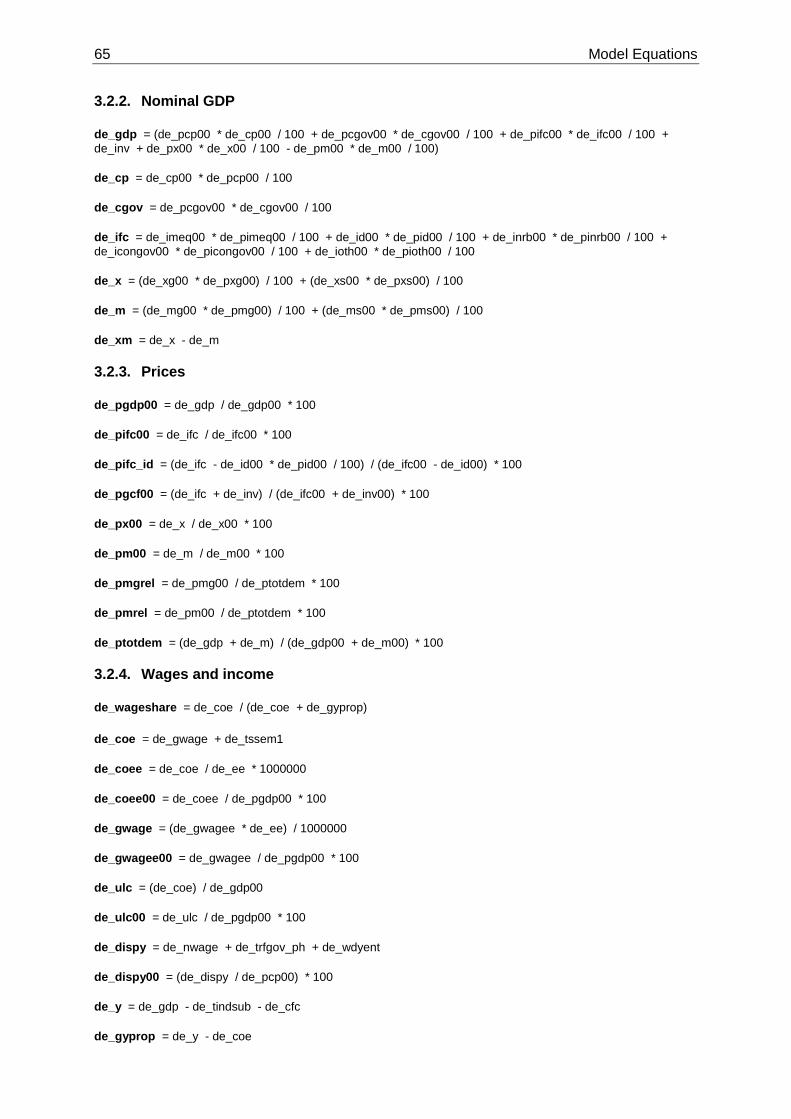
65 Model Equations

3.2.2. Nominal GDP

de_gdp = (de_pcp00 * de_cp00 / 100 + de_pcgov00 * de_cgov00 / 100 + de_pifc00 * de_ifc00 / 100 + de_inv + de_px00 * de_x00 / 100 - de_pm00 * de_m00 / 100)

de_cp = de_cp00 * de_pcp00 / 100

de_cgov = de_pcgov00 * de_cgov00 / 100

de_ifc = de_imeq00 * de_pimeq00 / 100 + de_id00 * de_pid00 / 100 + de_inrb00 * de_pinrb00 / 100 + de_icongov00 * de_picongov00 / 100 + de_ioth00 * de_pioth00 / 100

de_x = (de_xg00 * de_pxg00) / 100 + (de_xs00 * de_pxs00) / 100

de_m = (de_mg00 * de_pmg00) / 100 + (de_ms00 * de_pms00) / 100

de_xm = de_x - de_m

3.2.3. Prices

de_pgdp00 = de_gdp / de_gdp00 * 100

de_pifc00 = de_ifc / de_ifc00 * 100

de_pifc_id = (de_ifc - de_id00 * de_pid00 / 100) / (de_ifc00 - de_id00) * 100

de_pgcf00 = (de_ifc + de_inv) / (de_ifc00 + de_inv00) * 100

de_px00 = de_x / de_x00 * 100

de_pm00 = de_m / de_m00 * 100

de_pmgrel = de_pmg00 / de_ptotdem * 100

de_pmrel = de_pm00 / de_ptotdem * 100

de_ptotdem = (de_gdp + de_m) / (de_gdp00 + de_m00) * 100

3.2.4. Wages and income

de_wageshare = de_coe / (de_coe + de_gyprop)

de_coe = de_gwage + de_tssem1

de_coee = de_coe / de_ee * 1000000

de_coee00 = de_coee / de_pgdp00 * 100

de_gwage = (de_gwagee * de_ee) / 1000000

de_gwagee00 = de_gwagee / de_pgdp00 * 100

de_ulc = (de_coe) / de_gdp00

de_ulc00 = de_ulc / de_pgdp00 * 100

de_dispy = de_nwage + de_trfgov_ph + de_wdyent

de_dispy00 = (de_dispy / de_pcp00) * 100

de_y = de_gdp - de_tindsub - de_cfc

de_gyprop = de_y - de_coe

Model Equations 66

de_nwage = de_gwage - de_tdiree - de_tssee

de_masseneink = de_nwage + de_trfgov_ph

de_masseink00 = de_masseneink / de_pcp00 * 100

3.2.5. General government

de_tdir = de_tdiree + de_tdirem1

de_t = de_tdir + de_tind

de_tssem1 = de_gwage * de_tssem1_tariffsa_sa / 100

de_tssem = de_gwage * de_tssem_tariffsa_sa / 100

de_tssee = de_gwage * de_tssee_tariffsa_sa / 100

de_tss = de_tssee + de_tssem

de_revgov = de_t + de_tss + de_yprogov + de_revytrf + de_recprotr + de_salessub

de_expgov = de_cgov + de_intpagov + de_trfgov + de_protrgov + de_igov + de_subgov + de_trsongov + de_netprgov + de_expoth

de_bgov = de_revgov - de_expgov

deficit_gdp_ratio = de_bgov / de_gdp * 100

de_dbtgov = de_dbtgov(-1) - de_bgov

dbt_gdp_ratio = de_dbtgov / (de_gdp + de_gdp(-1) + de_gdp(-2) + de_gdp(-3)) * 100

3.2.6. Other variables

de_capital00 = de_capital00(-1) + de_imeq00 + de_inrb00 + de_icongov00 + de_ioth00 - de_cfc / de_pifc_id * 100 * .76 + i91q1 * 681

de_ur = (de_u ) / (de_et + de_u ) * 100

de_prodee = de_gdp00 / de_ee * 1000000

de_capa = (de_gdp00 / de_gdp00t) * 100

de_rl10y00 = de_rl10y - (de_pcp00 / de_pcp00(-4) - 1) * 100

de_rs3m00 = de_rs3m - (de_pcp00 / de_pcp00(-4) - 1) * 100

de_sav_ratio = 100 - de_cp / de_dispy * 100

de_reev_24_ptotdem = de_apeuro_24_ptotdem * de_ptotdem / 100

de_reev_56_cpi = de_apeuro_56_cpi * cpi_de / 100

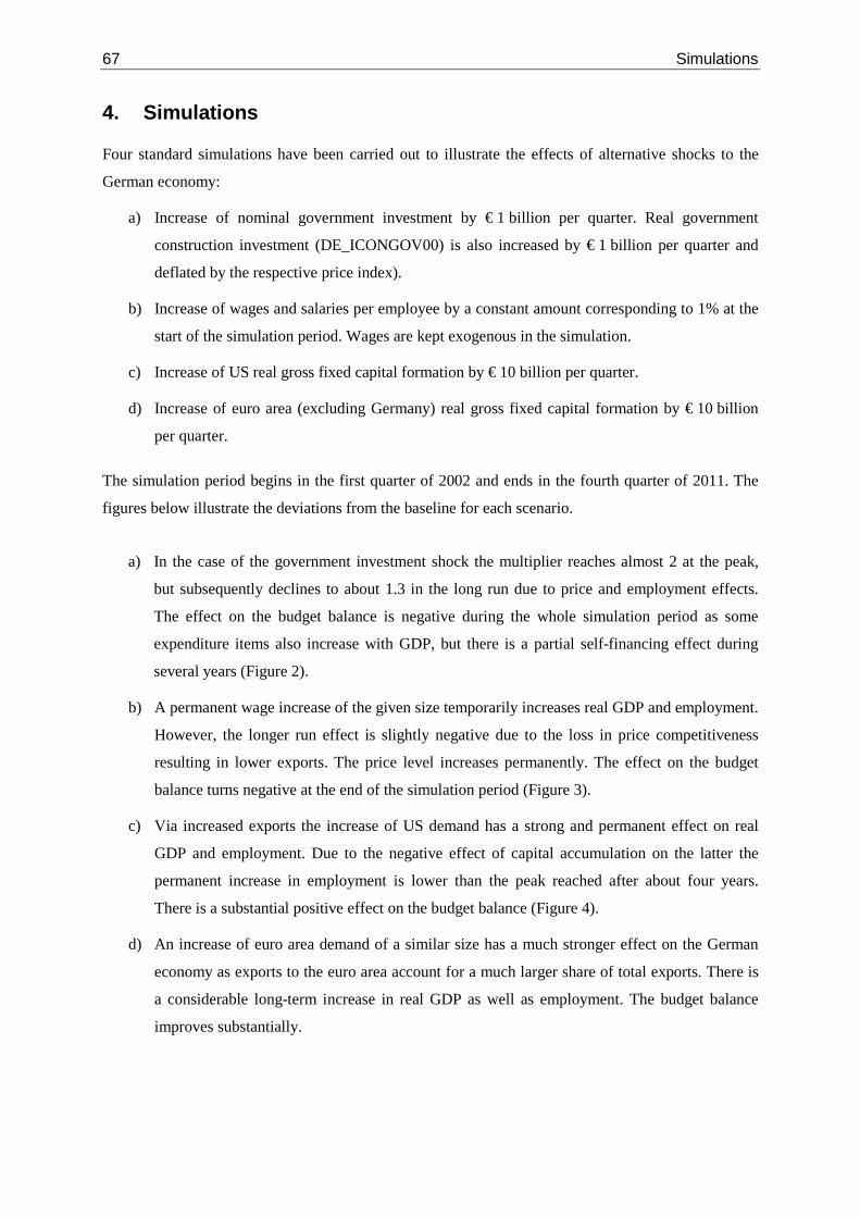
67 Simulations

4. Simulations

Four standard simulations have been carried out to illustrate the effects of alternative shocks to the

German economy:

a) Increase of nominal government investment by € 1 billion per quarter. Real government

construction investment (DE_ICONGOV00) is also increased by € 1 billion per quarter and

deflated by the respective price index).

b) Increase of wages and salaries per employee by a constant amount corresponding to 1% at the

start of the simulation period. Wages are kept exogenous in the simulation.

c) Increase of US real gross fixed capital formation by € 10 billion per quarter.

d) Increase of euro area (excluding Germany) real gross fixed capital formation by € 10 billion

per quarter.

The simulation period begins in the first quarter of 2002 and ends in the fourth quarter of 2011. The

figures below illustrate the deviations from the baseline for each scenario.

a) In the case of the government investment shock the multiplier reaches almost 2 at the peak,

but subsequently declines to about 1.3 in the long run due to price and employment effects.

The effect on the budget balance is negative during the whole simulation period as some

expenditure items also increase with GDP, but there is a partial self-financing effect during

several years (Figure 2).

b) A permanent wage increase of the given size temporarily increases real GDP and employment.

However, the longer run effect is slightly negative due to the loss in price competitiveness

resulting in lower exports. The price level increases permanently. The effect on the budget

balance turns negative at the end of the simulation period (Figure 3).

c) Via increased exports the increase of US demand has a strong and permanent effect on real

GDP and employment. Due to the negative effect of capital accumulation on the latter the

permanent increase in employment is lower than the peak reached after about four years.

There is a substantial positive effect on the budget balance (Figure 4).

d) An increase of euro area demand of a similar size has a much stronger effect on the German

economy as exports to the euro area account for a much larger share of total exports. There is

a considerable long-term increase in real GDP as well as employment. The budget balance

improves substantially.

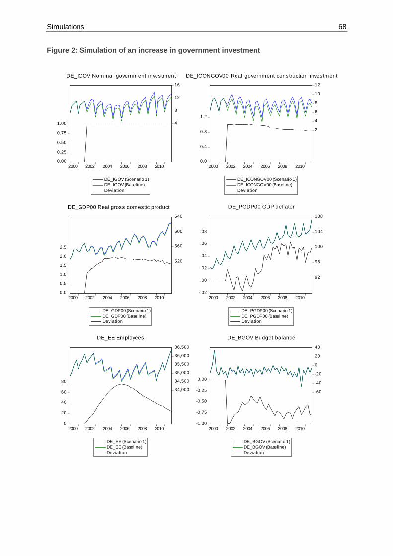
Simulations 68

Figure 2: Simulation of an increase in government investment

0.00

0.25

0.50

0.75

1.00 4

8

12

16

2000 2002 2004 2006 2008 2010

DE_IGOV (Scenario 1)DE_IGOV (Baseline)Deviation

DE_IGOV Nominal government investment

0.0

0.4

0.8

1.2

2

4

6

8

10

12

2000 2002 2004 2006 2008 2010

DE_ICONGOV00 (Scenario 1)DE_ICONGOV00 (Baseline)Deviation

DE_ICONGOV00 Real government construction investment

0.0

0.5

1.0

1.5

2.0

2.5

520

560

600

640

2000 2002 2004 2006 2008 2010

DE_GDP00 (Scenario 1)DE_GDP00 (Baseline)Deviation

DE_GDP00 Real gross domestic product

-.02

.00

.02

.04

.06

.08

92

96

100

104

108

2000 2002 2004 2006 2008 2010

DE_PGDP00 (Scenario 1)DE_PGDP00 (Baseline)Deviation

DE_PGDP00 GDP deflator

0

20

40

60

80

34,000

34,500

35,000

35,500

36,000

36,500

2000 2002 2004 2006 2008 2010

DE_EE (Scenario 1)DE_EE (Baseline)Deviation

DE_EE Employees

-1.00

-0.75

-0.50

-0.25

0.00

-60

-40

-20

0

20

40

2000 2002 2004 2006 2008 2010

DE_BGOV (Scenario 1)DE_BGOV (Baseline)Deviation

DE_BGOV Budget balance

69 Simulations

Figure 3: Simulation of a wage increase

0

20

40

60

80

5,500

6,000

6,500

7,000

7,500

8,000

8,500

2000 2002 2004 2006 2008 2010

DE_GWAGEE (Scenario 2)DE_GWAGEE (Baseline)Deviation

DE_GWAGEE Gross wages and salaries per employee

-0.5

0.0

0.5

1.0

1.5

520

560

600

640

2000 2002 2004 2006 2008 2010


DE_GDP00 Real gross domestic product

-1.6

-1.2

-0.8

-0.4

0.0 150

200

250

300

350

2000 2002 2004 2006 2008 2010

DE_X00 (Scenario 2)DE_X00 (Baseline)Deviation

DE_X00 Real exports

.0

.1

.2

.3

90

95

100

105

110

2000 2002 2004 2006 2008 2010

DE_PCP00 (Scenario 2)DE_PCP00 (Baseline)Deviation

DE_PCP00 Private consumption deflator

-20

0

20

40

60 34,400

34,800

35,200

35,600

36,000

36,400

2000 2002 2004 2006 2008 2010


DE_EE Employees

-0.4

0.0

0.4

0.8

1.2

-60

-40

-20

0

20

40

2000 2002 2004 2006 2008 2010



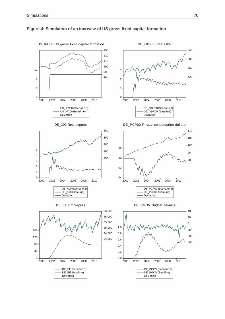
Simulations 70

Figure 4: Simulation of an increase of US gross fixed capital formation

0

4

8

12

80

90

100

110

120

130

2000 2002 2004 2006 2008 2010

US_IFC00 (Scenario 3)US_IFC00 (Baseline)Deviation

US_IFC00 US gross fixed capital formation

0

1

2

3

520

560

600

640

2000 2002 2004 2006 2008 2010


DE_GDP00 Real GDP

0

1

2

3

4

5

150

200

250

300

350

2000 2002 2004 2006 2008 2010


DE_X00 Real exports

-.04

-.02

.00

.02

90

95

100

105

110

2000 2002 2004 2006 2008 2010



0

40

80

120

160

34,000

34,500

35,000

35,500

36,000

36,500

2000 2002 2004 2006 2008 2010


DE_EE Employees

0.0

0.2

0.4

0.6

0.8

1.0

-60

-40

-20

0

20

40

2000 2002 2004 2006 2008 2010



71 Simulations

Figure 5: Simulation of an increase of EMU gross fixed capital formation

0

4

8

12

80

100

120

140

160

2000 2002 2004 2006 2008 2010

EWU_ODE_IFC00 (Scenario 4)EWU_ODE_IFC00 (Baseline)Deviation

EWU_ODE_IFC00 Gross fixed capital formationof the euro area excluding Germany

0

2

4

6

8

10

520

560

600

640

2000 2002 2004 2006 2008 2010


DE_GDP00 Real GDP

0

4

8

12150

200

250

300

350

2000 2002 2004 2006 2008 2010


DE_X00 Real exports

-.12

-.08

-.04

.00

.04

90

95

100

105

110

2000 2002 2004 2006 2008 2010



0

100

200

300

400

500

34,000

35,000

36,000

37,000

2000 2002 2004 2006 2008 2010


DE_EE Employees

0

1

2

3

-60

-40

-20

0

20

40

2000 2002 2004 2006 2008 2010



Conclusion 72

5. Conclusion

The IMK’s macroeconometric model of the German economy has been used for the IMK’s forecasts

as well as policy simulations for several years now. During this time individual equations have been

re-estimated frequently and will be re-estimated again whenever new data become available. Thus, the

current specifications are not sacrosanct and this documentation is merely a snapshot of the state of the

model in the summer of 2012. Despite frequent re-estimations the general structure and model

philosophy have remained more or less the same over the years.

Generally, the model is highly aggregated and rather compact. It allows addressing a large number of

macroeconomic issues, but has limitations. For specific interests additional equations and variables are

therefore added temporarily. For example, the model was amended by a module for the pension

system to analyse the effects of pension reform on macroeconomic stability (Meinhardt et al. 2009).

This may be repeated in the case of other specific policy issues.

Next steps will concentrate on the role of income distribution for private consumption expenditure.

With the availability of quarterly data for the government sector some more substantial revisions of

the respective equations may also become necessary.

73 References

References Banerjee, A., J. Dolado, and R. Mestre (1998): Error-correction mechanism tests for cointegration in a single-equation framework," Journal of Time Series Analysis, 19, 267-283.

Barcellan, R. (1994): -ECOTRIM: a Program for Temporal Disaggregation of Time Series," Paper presented at the joint INSEE and Eurostat Quarterly National Accounts Workshop in Paris on December 5th and 6th, 1994.

Chow, G., and A. Lin (1971): Best linear unbiased interpolation, distribution and extrapolation of time series by related series," The Review of Economics and Statistics, (53), 372-375.

Duong, M.H., Logeay, C., Stephan, S., Yahnych, S., Zwiener, R. (2005): Modelling European Business Cycles (EBC Model): A Macroeconometric Model of Germany ; Version March 2005, DIW Berlin, Data Documentation 5.

Dickey, D., and W. Fuller (1979): Distribution of the Estimators for Autoregressive Time Series with a Unit Root," Journal of the American Statistical Association, 74, 427-431.

Enders, W. (2004): Applied Econometric Time Series. Wiley, second edition.

Engle, R., and C. Granger (1987): Co-integration and error-correction: Representation, estimation and testing," Econometrica, 55(2), 251-276.

Hassler, U. (2004): Leitfaden zum Testen und Schätzen von Kointegration," in Arbeiten mit ökonometrischen Modellen, ed. by W. Gaab, U. Heilemann, and J. Wolters, pp. 85-115. Physica-Verlag, Heidelberg.

Lütkepohl, H. (2004): Univariate Time Series Analysis," in Applied Time Series Econometrics, ed. by H. Lütkepohl, and M. Krätzig, pp. 8-85. Cambridge University Press.

Meinhardt, V., Rietzler, K. and Zwiener, R. (2009): Konjunktur und Rentenversicherung – gegenseitige Abhängigkeiten und mögliche Veränderungen durch diskretionäre Maßnahmen, IMK Studies 3/2009, Düsseldorf;

Perron, P. (1989): The Great Crash, the Oil Price Shock, and the Unit Root Hypothesis," Econometrica, 57(6), 1361-1401.

Perron, P., and T. Vogelsang (1993): Erratum," Econometrica, 61(1), 248-250.

Ramsey, J. (1969): Tests for specifcation errors in classical linear least-squares regression analysis," Journal of the Royal Statistical Society, 31, 350-371.

Stephan, S. (2002): German exports to the euro area," DIW Discussion Papers, No. 286.

Stephan, S. (2005a): Pricing-to-Market Effects in Foreign Trade Prices," IMK Working Paper, No. 7/2005.

Stephan, S. (2005b): Sind deutsche Warenimport preisunelastisch? Neue Antworten auf ein altes "Puzzle" .

Stock, J. (1987): Asymptotic properties of least squares estimators of cointegrating vectors," Econometrica, 55(5), 1035-1056.

Tödter, K.-H. (2005): Umstellung der deutschen VGR auf Vorjahrespreisbasis Konzept und Konsequenzen für die aktuelle Wirtschaftsanalyse sowie die ökonometrische Modellierung," Diskussionspapier, Reihe 1: Volkswirtschaftliche Studien, No. 31/2005.

White, H. (1980): A heteroskedastic-consistent covariance matrix estimator and a direct test for heteroskedasticity," Econometrica, 48, 817-838.

Appendix: Variables of the model 74

Appendix: Variables of the model

Table 99: List of variables

Abbreviation Explanation Source

CPI_DE Consumer price index, Germany OECD

CPI_EWU Consumer price index, euro area OECD

CPI_UK Consumer price index, United Kingdom OECD

CPI_US Consumer price index, United States of America OECD

DBT_GDP_RATIO Debt to GDP ratio IMK calculations

DE_APEURO_24_PTOTDEM Foreign price level (total demand) of 24 countries in euro terms IMK calculations

DE_APEURO_56_CPI Foreign price level (cpi) of 56 countries in euro terms IMK calculations

DE_BGOV Government budget balance Destatis, IMK

DE_CAPA Capacity utilisation IMK estimate

DE_CAPITAL00 Capital stock, in real terms, reference year 2005 IMK calculation

DE_CFC Consumption of fixed capital Destatis

DE_CGOV Government consumption, nominal Destatis

DE_CGOV00 Government consumption, in real terms, reference year 2005 Destatis

DE_COE Compensation of employees Destatis

DE_COEE Compensation per employee IMK calculation

DE_COEE00 Compensation per employee, in real terms, reference year 2005 IMK calculation

DE_CP Private consumption, nominal Destatis

DE_CP00 Private consumption, in real terms, reference year 2005 Destatis

DE_DBTGOV Government gross debt Destatis

DE_DISPY Disposable income of households and NPISH, nominal Destatis

DE_DISPY00 Disposable income of households and NPISH, in real terms, reference year 2005 Destatis

DE_EE Employees Destatis

DE_END00 Total final demand, in real terms, reference year 2005 IMK calculation

DE_ET Employment Destatis

DE_EXPGOV Government expenditure Destatis

DE_EXPOTH Other government expenditures Destatis, IMK calculation

DE_GCF00 Gross capital formation, in real terms, reference year 2005 Destatis

DE_GDP Gross domestic product, nominal Destatis

DE_GDP00 Gross domestic product, in real terms, reference year 2005 Destatis

DE_GDP00T Trend of real GDP IMK estimate

DE_GWAGE Gross wages and salaries Destatis

DE_GWAGEE Gross wage per employee IMK calculation

DE_GWAGEE00 Real gross wage per employee, reference year 2005 IMK calculation

DE_GYPROP Operating surplus and mixed income Destatis

DE_ICONGOV00 Gross fixed capital formation of the government, in real terms, reference year 2005

Destatis

75 Appendix: Variables of the model


DE_ID00 Gross fixed capital formation: residential construction of private sector, in real terms, reference year 2005

Destatis

DE_IEND00 Total final domestic demand (DE_END00 less exports), in real terms, reference year 2005

IMK calculation

DE_IFC Gross fixed capital formation, nominal Destatis

DE_IFC00 Gross fixed capital formation, in real terms, reference year 2005 Destatis

DE_IGOV Gross fixed capital formation: government Destatis

DE_IMEQ00 Gross fixed capital formation: machinery and equipment, in real terms, reference year 2005

Destatis

DE_INRB00 Gross fixed capital formation: non-residential construction of private sector, in real terms, reference year 2005

Destatis

DE_INTPAGOV Property income paid, government (i.e. interest payments) Destatis

DE_INV Changes in inventories and net acquisitions of valuables, nominal Destatis

DE_INV00 Changes in inventories and net acquisitions of valuables, in real terms, reference year 2005

Destatis

DE_IOTH00 Gross fixed capital formation: other products, in real terms, reference year 2005

Destatis

DE_M Imports of goods and services, nominal Destatis

DE_M00 Imports of goods and services, in real terms, reference year 2005 Destatis

DE_MASSEINK00 Mass income, in real terms, reference year 2005 Destatis

DE_MASSENEINK Mass income, nominal Destatis

DE_MG00 Imports of goods, in real terms, reference year 2005 Destatis

DE_MS00 Imports of services, in real terms, reference year 2005 Destatis

DE_NETPRGOV Government: net increase of valuables DE_NEV_EWU Nominal effective exchange rate vis-à-vis

euro area countries IMK calculation

DE_NEV_UK Nominal effective exchange rate vis-à-vis the United Kingdom IMK calculation

DE_NEV_US Nominal effective exchange rate vis-à-vis the United States of America IMK calculation

DE_NWAGE Net wages and salaries Destatis

DE_PCGOV00 Government consumption deflator; index: 2005=100 Destatis

DE_PCP00 Private consumption deflator; index: 2005=100 Destatis

DE_PGCF00 Deflator of gross capital formation; index: 2005=100 Destatis

DE_PGDP00 GDP deflator; index: 2005=100 Destatis

DE_PICONGOV00 Deflator of gross fixed capital formation: government construction; index: 2005=100

Destatis



DE_PID00 Deflator of gross fixed capital formation: private residential construction; index: 2005=100

Destatis

DE_PIFC00 Deflator of gross fixed capital formation: total; index: 2005=100 Destatis

DE_PIFC_ID Deflator of gross fixed capital formation (excluding residential construction); index: 2005=100

Destatis

DE_PIMEQ00 Deflator of gross fixed capital formation: machinery and equipment; index: 2005=100

Destatis

DE_PINRB00 Deflator of gross fixed capital formation: private non-residential construction; index: 2005=100

Destatis

DE_PIOTH00 Deflator of gross fixed capital formation: other products; index: 2005=100 Destatis

DE_PM00 Deflator of imports of goods and services; index: 2005=100 Destatis

DE_PMG00 Deflator of imports of goods; index: 2005=100 Destatis

DE_PMGREL Price level of goods imports relative to domestic price level IMK calculation

DE_PMREL Price level of imports relative to domestic price level; index: 2005=100 IMK calculation

DE_PMS00 Deflator of imports of services; index: 2005=100 Destatis

DE_POPUL Population Destatis DE_PRODEE Productivity per employee IMK calculation DE_PROTRGOV Property transfers paid by the government Destatis, IMK calculations DE_PTOTDEM Deflator of total demand Destatis

DE_PX00 Deflator of exports of goods and services; index: 2005=100 Destatis

DE_PXG00 Deflator of exports of goods; index: 2005=100 Destatis

DE_PXS00 Deflator of exports of services; index: 2005=100 Destatis

DE_RECPROTR Property transfers received by the government Destatis, IMK calculations

DE_REEV_24_PTOTDEM Real effective exchange rate vis-à-vis 24 industrialised countries (price index: deflator of total demand)

Deutsche Bundesbank

DE_REEV_56_CPI Real effective exchange rate vis-à-vis 56 countries (price index: consumer price index)

Deutsche Bundesbank

DE_REVGOV Government revenue Destatis, IMK calculations

DE_REVYTRF Other current transfers received by the government from the other sectors Destatis, IMK calculations

DE_RL10Y Nominal long term interest rate (10 years) Deutsche Bundesbank DE_RL10Y00 Real long term interest rate (10 years) Deutsche Bundesbank

DE_RS3M Nominal short term interest rate (3 months, money market rate) IMK calculation

DE_RS3M00 Real short term interest rate (3 months, money market rate) IMK calculation

DE_SALESSUB Sales and other revenues of the Destatis, IMK calculations

77 Appendix: Variables of the model

Abbreviation Explanation Source government

DE_SAV_RATIO Household savings ratio Destatis DE_SUBGOV Government subsidies Destatis, IMK calculations DE_T Taxes paid to the government Destatis, IMK calculations DE_TDIR Direct taxes Destatis, IMK calculations

DE_TDIREE Taxes on income and wealth paid by employees Destatis

DE_TDIREM1 Taxes on income and wealth paid by employers and self-employed households Destatis, IMK calculations

DE_TIND Taxes on production and imports Destatis DE_TIND_TARIFFSA_SA Seasonally adjusted indirect tax rate IMK calculations

DE_TINDSUB Taxes less subsidies on production and imports Destatis

DE_TRFGOV Monetary government transfers paid by the government Destatis, IMK calculations

DE_TRFGOV_PH Monetary government transfers received by households Destatis

DE_TRSONGOV Other current transfers paid by the government Destatis, IMK calculations

DE_TSS Social contributions paid to the government Destatis, IMK calculations

DE_TSSEE Social contributions paid by employees Destatis

DE_TSSEE_TARIFFSA_SA Employees' social security contribution rate (seasonally adjusted) IMK calculations

DE_TSSEM Social contributions paid by employers Destatis, IMK calculations DE_TSSEM1 Employers' social contributions Destatis, IMK calculations

DE_TSSEM1_TARIFFSA_SA

Employers' social contribution rate (seasonally adjusted, difference between compensation of employees and gross wages and salaries)

IMK calculations

DE_TSSEM_TARIFFSA_SA Employers' social contribution rate (seasonally adjusted, government accounts)

IMK calculations

DE_U Unemployed persons (thousands) Destatis DE_ULC Unit labour cost IMK calculation DE_ULC00 Real unit labour cost IMK calculation DE_UR Unemployment rate Destatis DE_WAGESHARE Wage share (as a fraction of 1) IMK calculation DE_WDYENT Distributed profits IMK calculation DE_X Exports of goods and services, nominal Destatis

DE_X00 Exports of goods and services, in real terms, reference year 2005 Destatis

DE_XG00 Exports of goods, in real terms, reference year 2005 Destatis

DE_XG00_EWU Exports of goods to the euro area, in real terms, reference year 2005 Destatis

DE_XG00_ROW Exports of goods to the rest of the world, in real terms, reference year 2005 Destatis

DE_XG00_UK Exports of goods to the UK, in real terms, reference year 2005 Destatis



DE_XG00_US Exports of goods to the United States, in real terms, reference year 2005 Destatis

DE_XM Net exports, nominal Destatis

DE_XM00 Net exports, in real terms, reference year 2005 IMK calculation

DE_XS00 Exports of services, in real terms, reference year 2005 Destatis

DE_Y National income Destatis

DE_YPROGOV Property income reveived by the government Destatis, IMK calculations

DEFICIT_GDP_RATIO Budget balance in % of GDP Destatis, IMK calculations

EWU6_ULC Unit labour cost of 6 euro area countries IMK calculation based on Eurostat data

EWU_ODE_IFC00 Real gross fixed capital formation of EMU excluding Germany; index: 2000=100

IMK calculation based on Eurostat data

OIL$ Oil price in USD IMF, EIA

ROW_GDP00 Real GDP of the Rest of the world; index: 2000=100

World Bank, IMK calculations

UK_GDP05_SB UK GDP, in real terms; index: 2005=100 Eurostat

UK_ULC Unit labour cost UK IMK calculation based on Eurostat data

US_IFC00 Gross fixed capital formation of the United States, in real terms; index: 2000=100 OECD

US_ULC Unit labour cost, USA OECD

79 List of Figures

List of Figures Figure 1: Structure of the IMK Model .................................................................................................... 6

Figure 2: Simulation of an increase in government investment ............................................................ 68

Figure 3: Simulation of a wage increase ............................................................................................... 69

Figure 4: Simulation of an increase of US gross fixed capital formation ............................................. 70

Figure 5: Simulation of an increase of EMU gross fixed capital formation .......................................... 71

List of Tables

Table 1: Results of the Augmented Dickey-Fuller Tests ........................................................................ 8

Table 2: Results of the Perron Tests ...................................................................................................... 12

Table 3: Estimation equation of ΔLOG(DE_CP00) .............................................................................. 14

Table 4: Diagnostics of estimation equation of ΔLOG(DE_CP00) ...................................................... 15

Table 5: Estimation equation of ΔLOG(DE_CGOV00) ....................................................................... 15

Table 6: Diagnostics of estimation equation of ΔLOG(DE_CGOV00) ................................................ 16

Table 7: Estimation equation of ΔLOG(DE_IMEQ00)......................................................................... 16

Table 8: Diagnostics of estimation equation of ΔLOG(DE_IMEQ00) ................................................. 17

Table 9: Estimation equation of ΔLOG(DE_ID00) .............................................................................. 17

Table 10: Diagnostics of estimation equation of ΔLOG(DE_ID00) ..................................................... 18

Table 11: Estimation equation of ΔLOG(DE_INRB00) ....................................................................... 18

Table 12: Diagnostics of estimation equation of ΔLOG(DE_INRB00) ................................................ 19

Table 13: Estimation equation of ΔLOG(DE_IOTH00) ....................................................................... 19

Table 14: Diagnostics of estimation equation of ΔLOG(DE_IOTH00) ................................................ 20

Table 15: Estimation equation of DE_INV00 ....................................................................................... 20

Table 16: Diagnostics of estimation equation of DE_INV00 ................................................................ 21

Table 17: Estimation equation of ΔLOG(DE_XG00_EWU) ................................................................ 21

Table 18: Diagnostics of estimation equation of ΔLOG(DE_XG00_EWU) ........................................ 22

Table 19: Estimation equation of ΔLOG(DE_XG00_UK) ................................................................... 22

Table 20: Estimation equation of ΔLOG(DE_XG00_UK) ................................................................... 23

Table 21: Estimation equation of ΔLOG(DE_XG00_US) .................................................................... 23

Table 22: Diagnostics of estimation equation of ΔLOG(DE_XG00_US) ............................................ 24

Table 23: Estimation equation of ΔLOG(DE_XG00_ROW) ................................................................ 24

Table 24: Diagnostics of estimation equation of ΔLOG(DE_XG00_ROW) ........................................ 25

Table 25: Estimation equation of ΔLOG(DE_XS00) ............................................................................ 25

Table 26: Diagnostics of estimation equation of ΔLOG(DE_XS00) .................................................... 26

Table 27: Estimation equation of ΔLOG(DE_MG00) .......................................................................... 26

List of Tables 80

Table 28: Diagnostics of estimation equation of ΔLOG(DE_MG00) ................................................... 27

Table 29: Estimation equation of ΔLOG(DE_MS00) ........................................................................... 27

Table 30: Diagnostics of estimation equation of ΔLOG(DE_MS00) ................................................... 28

Table 31: Estimation equation of ΔLOG(DE_PCP00) .......................................................................... 29

Table 32: Diagnostics of Estimation equation of ΔLOG(DE_PCP00) ................................................. 29

Table 33: Estimation equation of ΔLOG(DE_PCGOV00) ................................................................... 30

Table 34: Diagnostics of Estimation equation of ΔLOG(DE_PCGOV00) ........................................... 30

Table 35: Estimation equation of LOG(DE_PIMEQ00) ....................................................................... 31

Table 36: Diagnostics of estimation equation of LOG(DE_PIMEQ00) ............................................... 31

Table 37: Estimation equation of ΔLOG(DE_PID00) .......................................................................... 32

Table 38: Diagnostics of Estimation equation of ΔLOG(DE_PID00) .................................................. 32

Table 39: Estimation equation of ΔLOG(DE_PINRB00) ..................................................................... 33

Table 40: Diagnostics of estimation equation of ΔLOG(DE_PINRB00) ............................................. 33

Table 41: Estimation equation of LOG(DE_PICONGOV00) ............................................................... 34

Table 42: Diagnostics of estimation equation of LOG(DE_PICONGOV00) ....................................... 34

Table 43: Estimation equation of ΔLOG(DE_PIOTH00) ..................................................................... 35

Table 44: Diagnostics of estimation equation of ΔLOG(DE_PIOTH00) ............................................. 35

Table 45: Estimation equation of ΔLOG(DE_PXG00) ......................................................................... 36

Table 46: Diagnostics of estimation equation of ΔLOG(DE_PXG00) ................................................. 36

Table 47: Estimation equation of ΔLOG(DE_PXS00) ......................................................................... 37

Table 48: Diagnostics of estimation equation of ΔLOG(DE_PXS00) .................................................. 37

Table 49: Estimation equation of ΔLOG(DE_PMG00) ........................................................................ 38

Table 50: Diagnostics of estimation equation of ΔLOG(DE_PMG00) ................................................. 38

Table 51: Estimation equation of ΔLOG(DE_PMS000) ....................................................................... 39

Table 52: Diagnostics of estimation equation of ΔLOG(DE_PMS000) ............................................... 39

Table 53: Estimation equation of LOG(CPI_DE) ................................................................................. 40

Table 54: Diagnostics of estimation equation of LOG(CPI_DE) .......................................................... 40

Table 55: Estimation equation of LOG(DE_CFC) ................................................................................ 41

Table 56: Diagnostics of estimation equation of LOG(DE_CFC) ........................................................ 41

Table 57: Estimation equation of ΔLOG(DE_TINDSUB) ................................................................... 42

Table 58: Diagnostics of estimation equation of ΔLOG(DE_TINDSUB) ............................................ 42

Table 59: Estimation equation of ΔLOG(DE_GWAGEE) ................................................................... 43

Table 60: Diagnostics of estimation equation of ΔLOG(DE_GWAGEE) ............................................ 44

Table 61: Estimation equation of ΔLOG(DE_EE) ................................................................................ 44

Table 62: Diagnostics of Estimation equation of ΔLOG(DE_EE) ........................................................ 45

Table 63: Estimation equation of ΔLOG(DE_ET) ................................................................................ 45

Table 64: Diagnostics of estimation equation of ΔLOG(DE_ET) ........................................................ 46

Table 65: Estimation equation of Δ(DE_U) .......................................................................................... 46

81 List of Tables

Table 66: Diagnostics of estimation equation of Δ(DE_U)................................................................... 47

Table 67: Estimation equation of ΔLOG(DE_WDYENT) ................................................................... 47

Table 68: Diagnostics of estimation equation of ΔLOG(DE_WDYENT) ............................................ 48

Table 69: Estimation equation of ΔLOG(DE_TRFGOV_PH) .............................................................. 48

Table 70: Diagnostics of estimation equation of ΔLOG(DE_TRFGOV_PH) ...................................... 49

Table 71: Estimation equation of ΔLOG(DE_TRFGOV) ..................................................................... 50

Table 72: Diagnostics of estimation equation of ΔLOG(DE_TRFGOV) ............................................. 51

Table 73: Estimation equation of ΔLOG(DE_INTPAGOV) ................................................................ 51

Table 74: Diagnostics of estimation equation of ΔLOG(DE_INTPAGOV) ......................................... 52

Table 75: Estimation equation of LOG(DE_TRSONGOV).................................................................. 52

Table 76: Diagnostics of estimation equation of LOG(DE_TRSONGOV) .......................................... 53

Table 77: Estimation equation of LOG(DE_PROTRGOV) .................................................................. 53

Table 78: Diagnostics of estimation equation of LOG(DE_PROTRGOV) .......................................... 54

Table 79: Estimation equation of DE_NETPRGOV ............................................................................. 54

Table 80: Diagnostics of estimation equation of DE_NETPRGOV ..................................................... 55

Table 81: Estimation equation of LOG(DE_EXPOTH)........................................................................ 55

Table 82: Diagnostics of estimation equation of LOG(DE_EXPOTH) ................................................ 56

Table 83: Estimation equation of ΔLOG(DE_TIND) ........................................................................... 56

Table 84: Diagnostics of estimation equation of ΔLOG(DE_TIND) .................................................... 57

Table 85: Estimation equation of ΔLOG(DE_TDIREE)....................................................................... 57

Table 86: Diagnostics of estimation equation of ΔLOG(DE_TDIREE) ............................................... 58

Table 87: Estimation equation of ΔLOG(DE_TDIREM1) ................................................................... 58

Table 88: Diagnostics of estimation equation of ΔLOG(DE_TDIREM1) ............................................ 59

Table 89: Estimation equation of ΔLOG(DE_YPROGOV) ................................................................. 59

Table 90: Diagnostics of estimation equation of ΔLOG(DE_YPROGOV) .......................................... 60

Table 91: Estimation equation of DE_REVYTRF ................................................................................ 60

Table 92: Diagnostics of estimation equation of DE_REVYTRF ........................................................ 61

Table 93: Estimation equation of LOG(DE_RECPROTR) ................................................................... 61

Table 94: Diagnostics of estimation equation of LOG(DE_RECPROTR) ........................................... 61

Table 95: Estimation equation of DE_SALESSUB .............................................................................. 62

Table 96: Diagnostics of estimation equation of DE_SALESSUB ....................................................... 62

Table 97: Estimation equation of DE_INV ........................................................................................... 63

Table 98: Diagnostics of estimation equation of DE_INV .................................................................... 63

Table 99: List of variables ..................................................................................................................... 74

Publisher: Hans-Böckler-Stiftung, Hans-Böckler-Str. 39, 40476 Düsseldorf, Germany Phone: +49-211-7778-331, [email protected], http://www.imk-boeckler.de

IMK Studies is an online publication series available at: http://www.boeckler.de/imk_5023.htm

ISSN: 1861-2180 The views expressed in this paper do not necessarily reflect those of the IMK or the Hans-Böckler-Foundation. All rights reserved. Reproduction for educational and non-commercial purposes is permitted provided that the source is acknowledged.

mailto:[email protected]

mailto:[email protected]

http://www.boeckler.de/imk_5023.htm

Sabine-Kurzboeck

Schreibmaschinentext

Sabine-Kurzboeck


Sabine-Kurzboeck


Sabine-Kurzboeck


Sabine-Kurzboeck


Sabine-Kurzboeck


Sabine-Kurzboeck


Sabine-Kurzboeck


Sabine-Kurzboeck


Sabine-Kurzboeck


Sabine-Kurzboeck


Sabine-Kurzboeck


Sabine-Kurzboeck


Sabine-Kurzboeck


Sabine-Kurzboeck


Sabine-Kurzboeck


Sabine-Kurzboeck


Sabine-Kurzboeck


Sabine-Kurzboeck


Sabine-Kurzboeck


Sabine-Kurzboeck


Sabine-Kurzboeck


Sabine-Kurzboeck


Sabine-Kurzboeck


Sabine-Kurzboeck


Sabine-Kurzboeck


Sabine-Kurzboeck


Sabine-Kurzboeck


Sabine-Kurzboeck


Sabine-Kurzboeck


Sabine-Kurzboeck


Sabine-Kurzboeck


Sabine-Kurzboeck


Sabine-Kurzboeck


Sabine-Kurzboeck


Sabine-Kurzboeck


Sabine-Kurzboeck


Sabine-Kurzboeck


Sabine-Kurzboeck


Sabine-Kurzboeck


Sabine-Kurzboeck


Sabine-Kurzboeck


Sabine-Kurzboeck


Sabine-Kurzboeck


Sabine-Kurzboeck


Sabine-Kurzboeck


Sabine-Kurzboeck


Sabine-Kurzboeck


Sabine-Kurzboeck


Dieses Gutachten wurde am 07. Februar 2011 abgeschlossen.

Sabine-Kurzboeck


Sabine-Kurzboeck


Sabine-Kurzboeck


Sabine-Kurzboeck


Sabine-Kurzboeck


Sabine-Kurzboeck


Sabine-Kurzboeck


macroeconomic p olicy institute study - hans-böckler-stiftung · this imk study is a documentation...

Documents