macroeconomic dynamics of income growth: evidences … · · 2016-06-26macroeconomic dynamics of...

European Journal of Business, Economics and Accountancy Vol. 4, No. 5, 2016 ISSN 2056-6018

Progressive Academic Publishing, UK Page 60 www.idpublications.org

MACROECONOMIC DYNAMICS OF INCOME GROWTH: EVIDENCES FROM

ARDL BOUND APPROACH, GMM AND DYNAMIC OLS

Dr. Muhammad Mustafa

School of Business

South Carolina State University

Orangeburg, SC 29117

USA

Dr. Haile M Selassie

School of Business

South Carolina State University

Orangeburg, SC 29117

USA

ABSTRACT

Using the annual data from 1980 through 2015, and applying the Autoregressive Distributed

Lag (ARDL) Bound Approach, Dynamic OLS (DOLS) and Generalized Method of Moments

(GMM) methodologies, this paper attempts to identify some major macroeconomic drivers of

income growth in South Carolina. The ARDL Bounds testing approach, proposed by Pesaran,

Shin, and Smith (2001) has several advantages compared to widely used Johansen and

Juselius (1990) cointegration technique. One advantage is that it lends itself to estimating the

long-run relationship without requiring the pretesting of the presence of unit root. Also, the

error-correction modeling by the ARDL cointegration procedure facilitates both short-run and

the long-run causality. The long-run results show that capital investment, export, government

expenditure, and new business have significant positive effect on the growth of income. The

short run dynamic results confirm that capital investment, export, government expenditure

and new business establishment have significant and positive impact on income growth. The

long term estimates indicate that a 1% increase in capital investment, export, government

expenditures, and new business would increase income growth by 7.71, 33.7, 16.89, and 28.4

percent respectively. Also, GMM and Dynamic OLS estimates find capital investment,

export, government expenditures and new business have significant and positive impact on

income growth. The results imply a commitment to export promotion, capital investment,

government expenditures and new business are important ingredients for successful state

growth strategy.

Keywords: Income Growth, ARDL Bound Approach, DOLS, GMM.

INTRODUCTION

The per capita income of South Carolina lags behind the nation and most of the Southern

states (Figure 1). While Georgia, Florida, North Carolina, Tennessee, Virginia, and the US

average reached $40,000 or more in 2015, Alabama, Mississippi, and South Carolina are

behind the national average. According to the Bureau of Economic Analysis, the population

of South Carolina was closer to 5 million in 2015 and ranked 23rd

in the nation (BEA, March

2016). The same report indicates that the State had per capita personal income of $38,041.

This is ranked 47th

in the US. Since 2009 the per capita personal income of South Carolina as

a percent of the United States has been declining.

This trend and disparity of economic well-being of the state should be of great concern to

economic policy makers who are designing economic development strategies. In developing

strategies, it is important to know and understand the dynamic causalities or the factors that

influence per capita income so that intervention can take place to reverse trends by promoting

and enhancing programs that will boost the economic well-being of the state.



Source: Bureau of Economic Analysis (www.bea.gov).

This paper investigates the dynamic short-run and long-run relationship among the growth in

per capita income, and macroeconomic variables such as export, capital investment,

government expenditure and new business establishment. The panel unit root, ARDL

cointegration, dynamic OLS (DOLS), and Generalized Method of Moments (GMM)

estimation methodologies are applied for the period 1980-2015. To the best of our

knowledge, similar empirical studies are not available. The remainder of the paper provides a

brief review of directly related literature followed by empirical methodologies and data,

results, discussion and conclusions.

LITERATURE REVIEW

The theory of economic growth and development suggests that the long term per capita

income growth is dependent on the growth of macroeconomic variables such as capital

investment, the productivity of human resources, government expenditure, new business

establishments, the level of export activities and other economic activities. Solow (1957)

provides a framework of long-term determinants of economic growth as a function of

growth in capital and labor. According to Elmendorf and Mankiw (1998), reduced domestic

investment over a period of time will result in a smaller domestic capital stock, which in turn

implies lower output and income. In addition, reduced net foreign investment over a period of

time means that domestic residents will own less capital abroad (or that foreign residents will

own more domestic capital). In either case, the capital income of domestic residents will fall.

The need for South Carolina to improve the quality of its workforce in order to compete in

the global, knowledge-based economy was examined by Shannon (2007). The study finds

several factors that hinder the state to improve the quality of its workforce include the lack of

broad effective leadership and communication or strong relationships with economic

development organizations. The need to speed-up economic development in South Carolina

is examined by Harrell (2006). The study suggests that the state must redouble its economic

development efforts to stimulate job growth. The article outlines three steps. First, the need is

to aggressively recruit companies to South Carolina. This will help in creating better jobs.

Next is to identify and implement ways to help large and small South Carolina companies

thrive. Finally, the state must transform research universities into economic engines. It is

0

10,000

20,000

30,000

40,000

50,000

60,000

Figure 1. Per Capita Income of South Carolina, USA, and

Southern States for Selected Years

Year 2000 Year 2005 Year 2010 Year 2015



going to take the cooperation of government and business leaders to transform the state to a

knowledge-based economy.

Hammond and Thompson (2006) found little role for public capital investment in either

metropolitan or non-metropolitan regions, but that manufacturing investment tended to spur

growth in non-metropolitan regions, in contrast to results for metropolitan regions. Further,

the study finds some evidence which suggests that human capital investment (measured by

college-level educational attainment) may not have a significant positive impact on growth in

non-metropolitan labor market areas, in contrast to metropolitan areas. However, these results

are only suggestive. The issue of global competition and public policy response is analyzed

by Barkley, Henry and Nair (2006). The study suggests the creation of a geographic

concentration of innovative activity (regional innovation systems [RIS]) that will enhance

metropolitan economic development through knowledge spillovers, product development,

and new firm spin-offs. This article identifies three RIS in the thirteen southern states based

on cluster analysis of twenty indicators of innovative and entrepreneurial activity.

The impact of policy to attract investors plays crucial role. For example, Miley and

Associates (2010) make a note of the great impact of Boeing and BMW’s investments on

manufacturing employment and gross state product. The study indicates that these two

investments have significant impact on South Carolina’s manufacturing jobs, and incomes of

the people. Similarly, Kuker (2011) offers an analysis of incentives to the Boeing Company

of South Carolina such as the House Bill 3130 that provides benefits including tax

exemptions and economic development bonds enjoyed by the Airbus SAS and Boeing.

Woodward (2013) uses South Carolina's economic development experience as a case study of

significant challenge in regional development. The study urges caution regarding

development incentives as a regional strategy and suggests that stronger agglomeration and

cluster-based strategies are better suited to promote economic development. Meacham (2010)

examines economic development policies created in North and South Carolina to attract

aircraft industry manufacturing facilities.

METHODOLOGY

Cointegration- ARDL Bounds Testing Approach

This study uses the ARDL bounds testing approach introduced by Pesaran and Shin (1999)

and extended by Pesaran, Shin and Smith (2001) to investigate the co-integration relationship

among capital investment, export, government expenditure, new business and income growth.

This test has several advantages over previous co-integration tests, such as the residual-based

technique by Robert and Granger (1987) and Full Maximum Likelihood (FML) test based on

Johansen (1988, 1991) and on Johansen and Juselius (1990). First, unlike other co-integration

techniques, the ARDL bounds testing approach does not impose the restrictive assumption

that all the variables under study must be integrated of the same order. The ARDL approach

can be applied to test the existence of a co-integrating relationship among variables

regardless of whether the underlying repressors are integrated of order one [I(1)], order zero

[I(0)], or fractionally integrated.

Second, conventional co-integration methods estimate the long-run relationships within the

context of a system of equations, the ARDL method employs only a single reduced form

equation (Pesaran & Shin, 1999). Third, the ARDL technique generally provides unbiased

estimates of the long-run model and valid t statistics – even when some of the regressors are



endogenous (Odhiambo, 2007; Odhiambo, 2010). Fourth, while other co-integration

techniques are sensitive to the size of the sample, the ARDL test is suitable even when the

sample size is small. Thus, the ARDL test has superior small sample properties compared to

the Johansen and Juselius (1990) co-integration test. Consequently, the approach is

considered very suitable for analyzing the underlying relationship and it has been

increasingly used in empirical research in recent years. Based on the previous studies and the

availability of data, the following double-log model is specified.

Where, LNPIt = natural log of Personal Income; LCINt = natural log of capital investment,

LSEXt = natural log of South Carolina export, LSGEt = Natural log of South Carolina

government expenditure, and LNBEt = Natural log of new business. A priori expected signs

of coefficients are >0, >0 and > 0. An ARDL representation of equation (1) is

Where Δ is the first difference, the parameters ij are the short-run parameters and ij are the

long run multipliers respectively in equation (2). The null and alternative hypotheses are:

Once the selected long run model is estimated, then the short run dynamic elasticities of the

variable within the framework of the errors-correction representation of the ARDL model is

estimated as follows in equation 3.

Where Φi is the speed of adjustment and E is the residual obtained from equation (2)

Dynamic OLS (DOLS)

The ARDL co-integration test is complimented with the dynamic OLS (DOLS) estimates.

The panel Dynamic Ordinary Least Squares (DOLS) methodology will provide the

estimation of the statistic long-run relation augmented by leads and lags. This will improve

the efficiency of the long-run estimates but does not provide guidance on the short-run

behavior. The following model is estimated:

(4)

GMM method

This paper also uses the GMM methodology developed by Arellano and Bond (1991) and

Arellano and Bover (1995). The advantage of this methodology is that it points out the



econometric problems caused by unobserved effects and endogeneity of the independent

variables in lagged–dependent-variable models such as income growth. This methodology

allows the relaxing of strong erogeneity of the explanatory variables by allowing them to be

correlated with current and previous realizations of the error term. The following model is

estimated:

(5)

RESULTS

Data and Sources

Annual data from 1980 through 2015 are employed. Personal income (NPI) capital

Investment (CIN), export (SEX), government expenditure(SGE) and New Business (NBE)

data from Bureau of Economic Analysis, SC Department of Commerce, Bureau of

Economic Analysis, US Census Bureau and SC Department of Commerce respectively.

Stationarity Tests

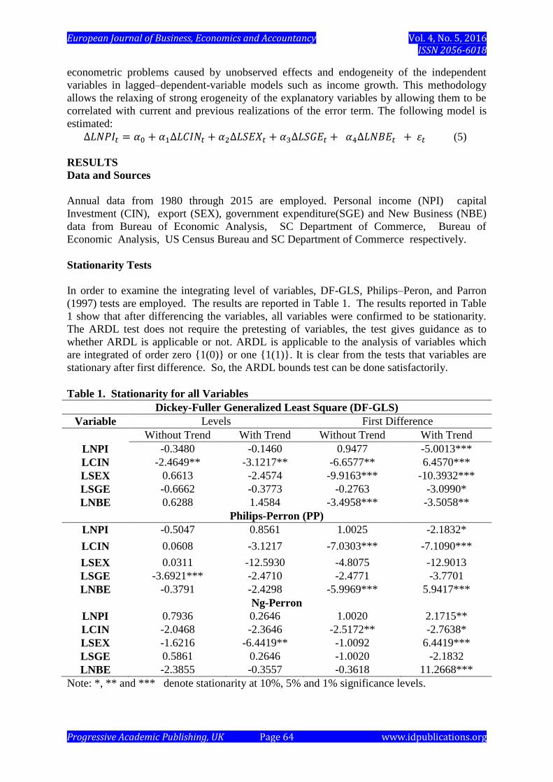
In order to examine the integrating level of variables, DF-GLS, Philips–Peron, and Parron

(1997) tests are employed. The results are reported in Table 1. The results reported in Table

1 show that after differencing the variables, all variables were confirmed to be stationarity.

The ARDL test does not require the pretesting of variables, the test gives guidance as to

whether ARDL is applicable or not. ARDL is applicable to the analysis of variables which

are integrated of order zero {1(0)} or one {1(1)}. It is clear from the tests that variables are

stationary after first difference. So, the ARDL bounds test can be done satisfactorily.

Table 1. Stationarity for all Variables

Dickey-Fuller Generalized Least Square (DF-GLS)

Variable Levels First Difference

Without Trend With Trend Without Trend With Trend

LNPI -0.3480 -0.1460 0.9477 -5.0013***

LCIN -2.4649** -3.1217** -6.6577** 6.4570***

LSEX 0.6613 -2.4574 -9.9163*** -10.3932***

LSGE -0.6662 -0.3773 -0.2763 -3.0990*

LNBE 0.6288 1.4584 -3.4958*** -3.5058**

Philips-Perron (PP)

LNPI -0.5047 0.8561 1.0025 -2.1832*

LCIN 0.0608 -3.1217 -7.0303*** -7.1090***

LSEX 0.0311 -12.5930 -4.8075 -12.9013

LSGE -3.6921*** -2.4710 -2.4771 -3.7701

LNBE -0.3791 -2.4298 -5.9969*** 5.9417***

Ng-Perron

LNPI 0.7936 0.2646 1.0020 2.1715**

LCIN -2.0468 -2.3646 -2.5172** -2.7638*

LSEX -1.6216 -6.4419** -1.0092 6.4419***

LSGE 0.5861 0.2646 -1.0020 -2.1832

LNBE -2.3855 -0.3557 -0.3618 11.2668***

Note: *, ** and *** denote stationarity at 10%, 5% and 1% significance levels.


Progressive Academic Publishing, UK 5 www.idpublications.org

Estimates of Unrestricted ARDL Model

Table 2 presents the unrestricted ARDL model estimates of equation (2). The model is

referred to as unrestricted equilibrium correction model. The long-run parameters and

respective standard errors are estimated using OLS. The table shows values of long-run ( and short run ( ) with their t-statistics. The coefficients of income growth lagged 1 period

(LNPI(-1)), capital investment (LCIN), export (LSEX) and Government Expenditure

(LSGE), and new business (LNBE) have positive and significant impact on economic growth.

Table 2: Unrestricted Estimates of ARDL Model (1, 0, 0, 0, 0)

Variable Coefficient Std. Error t-Statistic Prob.

LNPI(-1) 0.775503 0.076141 10.18503 0.0000

LCIN 0.017326 0.007660 2.261954 0.0314

LSEX 0.075683 0.030402 2.489382 0.0188

LSGE 0.037907 0.021375 1.773443 0.0867

LNBE 0.063772 0.039352 1.620569 0.1159

C 0.675419 0.323159 2.090049 0.0455

R2 0.999249 Schwarz criterion -4.886694

Adjusted R2 0.999120 F-statistic 7721.386

Co-integration and ARDL-ECM Bound Test

The long-run relationship among the variables in the general model is examined using the

ARDL bounds testing procedure. The first step is to obtain the order of lags on the first

differenced variables in equations (2) by using the Schwartz Bayesian Criterion. This is

followed by the application of a bound F-test to equation (2) to establish a long-run

relationship between the variables under study. The results of the bounds F-test are reported

in table 3.

Table 3: ARDL Bounds Test for Cointegration

Null Hypothesis: No long-run relationships exist

Test Statistic Value k

F-statistic 57.46270 4

Critical Value Bounds

Significance I0 Bound I1 Bound

10% 2.2 3.09

5% 2.56 3.49

2.5% 2.88 3.87

1% 3.29 4.37

The results of the F-test suggest that there exists a long-run relationship among LNPI,

LCIN, LSEX, LSGE and LNBE. Therefore, the empirical findings lead to the conclusion that

a long run relationship among income growth, capital investment, export, government

expenditure and new business exist.

The above result is a step forward to the estimation of long-run coefficients which are

reported in Table 4. The long-run estimated coefficients of capital investment, new business

are significant at 5% level and the coefficients of export and government expenditure are

significant at 1% level. The result of long run estimated coefficients show that a one percent



increase in capital investment, export, government expenditure, and new business is expected

to lead to 7.7, 33.7, 16.9 and 28.4% increase in income growth respectively.

Table 4: Long Run ARDL Cointegration Model (1, 0, 0, 0, 0, 0)

Long Run Coefficients


LCIN 0.077178 0.038567 2.001160 0.0548**

LSEX 0.337123 0.055582 6.065287 0.0000*

LSGE 0.168852 0.055046 3.067470 0.0046*

LNBE 0.284069 0.136569 2.080036 0.0465**

C 3.008589 1.369972 2.196096 0.0362**

Note: Asterisk *, ** Show significance levels at the 1%, and 5% level

Diagnostic Tests:

Adjusted R2 0.9900

JB Normality Test 0.8811(0.6436)

Breusch-Godfrey Serial Correlation F-Test: 1.07288(0.3561)

Breusch-Pagan-Godfrey Heteroscedasticity F-Test 0.2840 (09163)

In Table 4, the results of the estimated long-run ARDL cointegration model (1, 0, 0, 0, 0),

selected automatically by Schwarz criterion (SIC) out of 2500 models are reported. The SIC

criterion automatically determined the lag to be one. The bottom portion of Table 4 displays

the results of the diagnostic tests of the selected ARDL (1, 0, 0, 0, 0) model. The coefficient

of adjusted degree of freedom, R2,

is 99%, explaining the variation in income growth by

changes in LCIN, LSEX, LSGE, and LNBE. The JB test for normality indicates that the

residual are normality distributed. Breusch-Godfrey Serial Correlation F-test and the

Breusch-Godfrey Heteroskedasticity F-test fail to reject the null-hypothesis of no serial

correlation and no heteroscedasticity of the residuals.

Table 5 is drawn from Table 4 to emphasize the estimated coefficients are also the elasticities

of the macroeconomic variables with respect to income growth. The results indicate the

elasticities of capital investment, export, government expenditure, and new business with

respect to income growth are 0.0771, 0.3370, 0 .1689, and 0.2840 respectively. The results

imply that a one percent increase in capital investment, export, government expenditures, and

new business establishment would be expected to increase income growth by 7.71, 33.7,

16.89, and 28.4 percent respectively.

Table 5: Elasticity Estimates with Respect to Income Growth

Capital Investment 0.0771**

Export 0.3370*

Government Expenditure 0.1689*

New Business 0.2840**

Note: Asterisks *, ** Show significance levels at the 1%, and 5% level

In table 6, the results of the estimated ARDL short-run error-correction model is presented.

The coefficients of ∆LCIN, ∆ LSEX, ∆LSGE and ∆LNBE exhibited a positive sign and are

significant at 1%, 1%, 5% and 8% respectively. The coefficient of error-correction term, ECT

(-1), is significant at the 1% level and exhibits the expected negative sign. The error-

correction term, besides confirming the existence of cointegration based on the ARDL model,



shows that 21% of the disequilibria in the income growth arising out of past shocks will be

corrected in the current period, although the speed of adjustment is relatively slower.

Table 6: The ARDL Cointegrating Short-run Error-Correction Model (1, 0, 0, 0, 0)


∆(LCIN) 0.023127 0.007344 3.149005 0.0038

∆ (LSEX) 0.090181 0.033685 2.677231 0.0121

∆ (LSGE) 0.036554 0.018622 1.962915 0.0593

∆ (LNBE) 0.067334 0.037216 1.809284 0.0808

ECT(-1) -0.217650 0.019819 -10.981679 0.0000

Parameter stability tests

One of the requirements for well-specified ARDL model is the presence of stability of

parameter. One should always employ the cumulative sum of recursive residuals (CUSUM)

and cumulative sum of squares of recursive residuals (CUSUMQ) as suggested in Brown,

Durbin, and Evans (1975). Figures 2 and 3 report plots of the CUSUM and CUSUMSQ

graphs. It can be seen that the plot of CUSUM and CUSUMQ stay within the critical 5%

bounds. This confirms the long-run relationships among variables and thus indicates the

stability of coefficients.

Figure 2: CUSUM test for stability

-16

-12

-8

-4

0

4

8

12

16

88 90 92 94 96 98 00 02 04 06 08 10 12 14

CUSUM 5% Significance



Figure 3: CUSUM Square Test for Stability

-0.4

-0.2

0.0

0.2

0.4

0.6

0.8

1.0

1.2

1.4

88 90 92 94 96 98 00 02 04 06 08 10 12 14

CUSUM of Squares 5% Significance

Dynamic OLS (DOLS)

To complement the ARDL co-integration test, the dynamic OLS (DOLS) is estimated. The

panel Dynamic Ordinary Least Squares (DOLS) methodology will provide the estimation of

the statistic long-run relation augmented by leads and lags. This will improve the efficiency

of the long-run estimates but does not provide guidance on the short-run behavior. The

estimated results are reported in Table 7. The coefficients of capital investment, export,

government expenditure, and new business all are positive and significant at 1% level,

suggesting that in the long run they will lead the income growth rate.

Table 7: Dynamic Least Squares (DOLS)


LCIN 0.036034 0.010955 3.289147 0.0046

LSEX 0.384571 0.016767 22.93633 0.0000

LSGE 0.090381 0.027484 3.288519 0.0046

LNBE 0.784813 0.104364 7.519939 0.0000

C -2.203768 0.955527 -2.306339 0.0348

R2 0.999540 Adjusted R

2 0.999080

GMM Estimates

The results of the GMM estimates are reported in Table 8. The coefficients of capital

investment, export, and new business are positive and significant at 1% level suggesting that

they will lead the income growth rate. Thus, both dynamic OLS cointegration and GMM

estimates lead to almost identical conclusion. However, in the GMM estimates, the estimated

coefficients of explanatory variables are usually taken to represent short-term impact, whilst

dynamic OLS (DOLS) estimates provide information on the long-run. Also, capital

investment is positive in both models and significant in dynamic OLS.



Table 8: Generalized Method of Moments (GMM)


LCIN 0.036394 0.038079 0.955764 0.3466

LSEX 0.312275 0.040315 7.745824 0.0000

LSGE 0.217029 0.042517 5.104481 0.0000

LNBE 0.537722 0.023875 22.52227 0.0000

R2 0.995186 J-statistic 1.548240

Adjusted R2 0.994720

DISCUSSION

This paper, for the first time in the literature, has applied the ARDL bound approach,

dynamic OLS, and GMM method to empirically identify major macroeconomic drivers of

personal income growth in South Carolina during the period of 1980-2015. ARDL bound

approach and dynamic OLS (DOLS) show that major drivers of income growth in South

Carolina are capital investment, export, government expenditures and new business. The

study shows all the variables are stationary at level or after first difference. Hence, they are

integrated of order I (1). Together they form a long-run link exhibiting an integrating

relationship among LNPI, LCIN, LSEX, LSGE and LNBE. The coefficients of all variables

in ARDL short-run estimates and GMM estimates are positive and significant with the

exception of LCIN in the GMM model. The coefficient of error-correction, ECT (-1) is

significant at 1% level and has negative sign as expected.

The elasticities of capital investment, export, government expenditures, and new business

establishment with respect to income growth are 0.077, 0.337, 0.1689, and 0.284

respectively. In other words, the result imply that one percent increase in capital investment,

export, government expenditures, and new business establishment would be expected to

increase by 7.7, 33.7, 16.9, and 28.4 percent respectively.

CONCLUSION

This paper investigates the dynamic short-run and long-run relationship among the growth in

per capita income, and macroeconomic variables such as export, capital investment,

government expenditure and new business establishment. The panel unit root, ARDL bound

cointegration, dynamic OLS (DOLS), and Generalized Method of Moments (GMM)

estimation are applied for the period 1980-2015. The long-run results show that capital

investment, export, government expenditure, and new business have significant positive

effect on the growth of income. The short run dynamic results confirm that capital

investment, export, government expenditure and new business establishment have significant

positive impact on income growth. The long term estimates indicate that a 1% increase in

capital investment, export, government expenditures and new business would be expected to

increase income growth by 7.71, 33.70, 16.89, and 28.40 percent respectively. Also, GMM

estimates, which represent short run impact, find capital investment, export, government

expenditures and new business have significant and positive impact on income growth. The

estimated ARDL cointegration model passes the econometric diagnostic tests. Also,

coefficients are stable. CUSUM and CUSUMQ tests confirm the long run stable relationship

among the variables. The results imply capital investment, export, new business, government

expenditures are macroeconomic drivers of economic growth. One of the policy implications

of the findings in this paper is that policy makers should strategize to encourage capital



investment, attract new businesses like BMW, Boeing and Amazon.com and promote

exports.

ACKNOWLEDGEMENTS

This article is based upon work that is supported by the National Institute of Food and

Agriculture, U.S. Department of Agriculture, Evans-Allen project number SCX-101-08-15.

Any opinions, findings, conclusions, or recommendations expressed in this publication are

those of the authors and do not necessarily reflect the view of the U.S. Department of

Agriculture.

REFERENCES

Arellano, M. and Bond, S. (1991). “Some Tests of Specification for Panel Data: Monte Carlo

Evidence and an Application to Employment Equations.” Review of Economic Studies,

58, 277-297.

Arellano, M. & Bover, O. (1995). Another Look at the Instrumental Variable Estimation of

Error Components Models. Journal of Econometrics, 68, 29-51.

Brown, R. L, J. Durbin and J. M. Evans (1975). Techniques for Testing the Constancy of

Regression Relationships over Time. Journal of the Royal Statistical Society. Series B

(Methodological). Vol. 37, No. 2 (1975), 149-192

Dickey, D.A., and W.A. Fuller (1979). Distribution of the Estimators for Autoregressive

Time Series with a Unit Root. Journal of the American Statistical Association, 74,

427-431.

Elmendorf D.W. and Mankiw N.G. (1998). Government Debt. Harvard Institute of Economic

Research, Research Paper.

Engle, Robert F. and C.W.J. Granger (1987). Co-integration and Error Connection:

Representation, Estimation, and Testing. Econometrica, Vol 55, No 2. (March 1987),

251-276.

Hammond G.W. and Thompson E. (2006) “Determinants of Income Growth in U.S.

Metropolitan and Non-Metropolitan Labor Markets”, West Virginia University.

Johansen, S. (1988). Statistical Analysis of Cointegration Vectors. Journal of Economic

Dynamics and Control, 12, 231-254.

Johansen S. (1991). Estimation and Hypothesis Testing of Cointegration Vectors in Gaussian

Vector Autoregressive Models. Econometrica. Published by the Econometrica Society.

Vol. 59, No. 6, 1551-1580.

Johansen, S., and Juselius, K. (1990). Maximum Likelihood Estimation and Inference on

Cointegration with Applications to the Demand for Money. Oxford Bulletin of

Economics and Statistics, 51, 69-210.

Kuker, A. (2011). “An Analysis of South Carolina's Incentives to Boeing Company."

Journal of International Law & Business, fall, Vol.8 Issue 1, 165-203.

Mecham, Michael. (2010). “Big Ambitions" Aviation Week & Space Technology, Vol. 172,

Issue 42, 50.

Ng, Serena and Pierre Perron (2001). Lag Length Selection and the Construction of Unit Root

Tests with Good Size and power. Econometrica, 69, 1519-1554.

Odhiambo, N. M. (2007). “Supply-leading versus Demand-following Hypothesis: Empirical

Evidence from SSA Countries,” African Development Review, 19, 257-280.

Odhiambo, N. M. (2010). “Financial Investment-Growth Nexus in South Africa: An ARDL-

bounds Testing Procedure”, Economic Change and Restructuring, 43, 205-219.



Pesaran, M.H., and Shin, Y., 1999. An Autoregressive Distributed Lag-Modelling

Approaches to Co-Integration Analysis, Chapter 11, in Econometrics and Economic

Theory in the 20th

Century: The Ragnar Frisch Centennial Symposium, Strom S.-

Cambridge University Press, Cambridge.

Pesaran, M. H., Y. Shin, and R. Smith (2001). Bounds Testing Approach to the analysis of

Level Relationships. Journal of Applied Economics, 16, 289-326.

Philips, P.C.B. and Perron (1988). Testing for a Unit Root in Time Series Regression.

Biometrika, 75, 335-346

Shannon, Sue-Ann Gerald. (2007). “Reshaping South Carolina's Workforce.” Business &

Economic Review, Jan Mar2007, Vol. 53 Issue 2, 3-6.

Solow, R.M. (1956). A Contribution to the Theory of Economic Growth. Quarterly Journal

of Economics (70), 65-94.

Woodard, Douglas. (2013). "Industry Location, Economic Development Incentives, and

Clusters" The Official Journal of the Southern Regional Science Association, 5, 23

macroeconomic dynamics of income growth: evidences … · · 2016-06-26macroeconomic dynamics of...

Documents