IFPRI Discussion Paper 00897 September 2009

Spatial Networks, Labor Supply, and Income Dynamics

Evidence from Indonesian Villages

Futoshi Yamauchi Megumi Muto

Shyamal Chowdhury Reno Dewina

Sony Sumaryanto

Poverty, Health, and Nutrition Division

brought to you by COREView metadata, citation and similar papers at core.ac.uk

provided by Research Papers in Economics

INTERNATIONAL FOOD POLICY RESEARCH INSTITUTE

The International Food Policy Research Institute (IFPRI) was established in 1975. IFPRI is one of 15 agricultural research centers that receive principal funding from governments, private foundations, and international and regional organizations, most of which are members of the Consultative Group on International Agricultural Research (CGIAR).

FINANCIAL CONTRIBUTORS AND PARTNERS IFPRI’s research, capacity strengthening, and communications work is made possible by its financial contributors and partners. IFPRI receives its principal funding from governments, private foundations, and international and regional organizations, most of which are members of the Consultative Group on International Agricultural Research (CGIAR). IFPRI gratefully acknowledges the generous unrestricted funding from Australia, Canada, China, Finland, France, Germany, India, Ireland, Italy, Japan, Netherlands, Norway, South Africa, Sweden, Switzerland, United Kingdom, United States, and World Bank.

AUTHORS Futoshi Yamauchi, International Food Policy Research Institute Research Fellow, Poverty, Health, and Nutrition Division Megumi Muto, Japan International Cooperation Agency Research Institute Research Fellow Shyamal Chowdhury, University of Sydney Lecturer, Department of Agriculture and Resource Economics Reno Dewina, International Food Policy Research Institute Research Analyst, Markets, Trade, and Institutions Division Sony Sumaryanto, Indonesian Center for Agriculture Socio Economic Policy Studies Researcher

Notices 1 Effective January 2007, the Discussion Paper series within each division and the Director General’s Office of IFPRI were merged into one IFPRI–wide Discussion Paper series. The new series begins with number 00689, reflecting the prior publication of 688 discussion papers within the dispersed series. The earlier series are available on IFPRI’s website at www.ifpri.org/pubs/otherpubs.htm#dp. 2 IFPRI Discussion Papers contain preliminary material and research results. They have not been subject to formal external reviews managed by IFPRI’s Publications Review Committee but have been reviewed by at least one internal and/or external reviewer. They are circulated in order to stimulate discussion and critical comment.

Copyright 2009 International Food Policy Research Institute. All rights reserved. Sections of this material may be reproduced for personal and not-for-profit use without the express written permission of but with acknowledgment to IFPRI. To reproduce the material contained herein for profit or commercial use requires express written permission. To obtain permission, contact the Communications Division at ifpri-copyright@cgiar.org.

iii

Contents

Acknowledgments v

Abstract vi

1. Introduction 1

2. Data 3

3. Descriptive Analyses 7

4. Empirical Framework 16

5. Empirical Results 17

6. Policy Discussion 21

7. Conclusion 22

References 23

iv

Tables 1. Sample village ecological and agricultural characteristics 4

2. Asphalt road proportions in intervillage roads (province-wise averages) 8

3. Village-level changes in intervillage road quality (asphalt/concrete/cone-block or not), 1996-2006 9

4. Distances to subdistrict, district, and provincial capitals 11

5. Summary statistics 12

6. Changes in nonagricultural income 18

7. Changes in labor supply to the nonagricultural sector 20

Figures 1. Locations of surveyed villages 3

2. Changes in average intervillage road quality (asphalt road proportion) 10

3a. Per capita income growth and household head’s education under conditions of improved road quality 14

3b. Per capita income growth and household head’s education under conditions of deteriorated road quality 14

4a. Changes in nonagricultural income share and average road quality 15

4b. Changes in nonagricultural labor income share and average road quality 15

v

ACKNOWLEDGMENTS

This study is based on collaboration of the Japan International Cooperation Agency (JICA), the International Food Policy Research Institute (IFPRI), and the Indonesian Center for Agriculture and Socio Economic Policy Studies (ICASEPS). The team acknowledges financial support from JICA. We are especially grateful to Ali Subandoro for his leadership in organizing the survey teams. We also thank all of the fieldworkers and team leaders who collected the survey data, as well as Takako Yuki, Shinobu Shimokoshi, and various workshop participants in the Indonesian Ministry of Agriculture for their helpful comments.

vi

ABSTRACT

This paper uses household panel and village census data from Indonesia to examine the impact of spatial connectivity (road) development on household income growth and nonagricultural labor supply. The empirical results show that the impacts of improvements in local road quality (which positively correlate with transportation speed) on income growth and the transition to nonagricultural labor markets depend on the distance to economic centers and the household education level. In particular, postprimary education significantly increases the benefit from local spatial connectivity improvement in remote areas and promotes labor transition to nonagricultural sectors. Education and local road quality are complementary, mutually increasing income growth and nonagricultural labor income in remote areas. The gain from improvements in local connectivity (measured by average road quality) depends on village remoteness and initial household-level endowments. Keywords: income growth, spatial connectivity, rural economy, education, Indonesia

1

1. INTRODUCTION

Economic growth often shows spatial inequality. Spatial connection to high growth centers can facilitate escape from poverty in local economies, largely by improving economic returns to investment and reducing the costs of transportation and acquisition of both human and physical resources, thereby altering household resource allocation. In general, improvement of spatial connectivity is expected to increase the allocative efficiency of the local economy, since the mobilization of resources becomes faster and less costly, thereby reducing price disparities (for example, Minten and Kyle 1999).

We herein seek to identify household behaviors (especially pertaining to labor supply) that dynamically respond to improvements in spatial connectivity, and examine how spatial connectivity affects household incomes, labor allocation, and the economic transition from a farm-based rural economy to nonfarm development. At present, it is not clear how better spatial connectivity (for example, among neighborhood local areas and/or with distant economic centers) can change income distribution in village economies. Furthermore, we do not yet fully understand what population(s) gain first from better spatial connectivity. However, improved spatial connectivity in the local economy may have heterogeneous impacts on households with different endowments. In this paper, we address these issues by focusing on household labor supplies in Indonesia, using a combination of two unique data sets: household panel data and village census data.1

Once a new road connects a rural village to a nearby town where jobs are available, the household allocation of labor in the rural village is expected to change as household members seek earning opportunities in the town’s labor market. If entry to the labor market is easier for educated agents, the allocation of labor will differ by the household level of education. More educated agents may try to capture better employment or urban market opportunities that are available in larger economic centers farther than the local town (without migrating). In this case, road access to the larger economic center becomes important. Thus, the effects of improved road quality could be heterogeneous across different locations and among households with different endowments.

2

The recent literature provides some studies suggesting that returns to human and physical capital in rural areas critically depend on spatial connectivity, which affects the allocation of household resources, including labor supply (for example, Fafchamps and Shilpi 2003, 2005; Fafchamps and Wahba 2006). Fafchamps and Shilpi (2003) show that the distance to cities crucially determines wage opportunities and employment structures in Nepal, with nonfarm employment (either wage or self-employment) concentrated in and around cities. Road construction, which improves the access to (nonagricultural) labor markets and/or urban consumers, increases wages and employment choices for rural residents. Furthermore, certain types of employment become newly available with improved spatial linkages.

3

1 Over the past three decades, Indonesia has transformed from a predominantly farm economy to one that relies heavily on

its nonfarm sector. The gross domestic product (GDP) per capita grew at an annual average rate of above 5 percent beginning in 1970 and lasting until just before the economic crisis. The relative contribution of agriculture to GDP declined from a share of around 45 percent in 1970 to around 16 percent in 2001 (World Bank 2003). However, these changes were unevenly distributed, with some regions lagging significantly behind then other regions. A similar pattern can be observed in spatial connectivity; some regions have made significant progress while others have lagged.

2 Developmental economics has placed enormous emphasis on labor supply and wage determination ever since the early contributions of Lewis (1954), Sen (1966), and Stiglitz (1974, 1976). Since the 1980s, neoclassical labor supply has been examined in numerous empirical studies (for example, Rosenzweig 1980 and Benjamin 1992), as summarized in Singh, Squire, and Strauss (1986). Fafchamps (1993) introduced a rigorous dynamic analysis in this area. To our knowledge, our work is the first attempt to analyze the role of spatial network development (as measured by changes in local road quality) on household labor supply behavior and income in a developing country.

3 The improvement of spatial connectivity also has implications for product markets, as it reduces transportation margins. Minten and Kyle (1999) show that price variations are largely due to transportation costs in the former Zaire. Interestingly, traders gain from bad road conditions, with reduced purchase prices increasing their profits. Therefore, spatial connectivity can potentially increase farmers’ incomes by reducing traders’ profit margins.

2

Connectivity to urban centers benefits laborer households more than farm (landed) households by improving access to nonagricultural employment opportunities. Foster and Rosenzweig (2001) show that the landless in India prefer road construction as a local public investment choice because it improves access to labor markets, whereas the landed prefer investment in irrigation, which augments returns to land. Infrastructure can bring changes in both farm and nonfarm production, and it can alter labor demand by changing production composition towards nonfarm and tertiary activities. Infrastructure can have both substitution and complementary effects; it can be a cheaper substitute for some inputs and can have positive complementarities with other inputs, potentially shifting production composition toward activities that use the infrastructural services. Moreover, by integrating fragmented markets, infrastructure can outwardly shift the production frontier, thereby increasing labor demand. By reducing the time and energy costs created by distance, and decreasing the transportation costs between rural and urban areas (and within rural areas), infrastructure can integrate fragmented markets.

Since Aschauer’s (1989a, 1989b) pioneering works on the effects of public infrastructure on productivity, a diverse body of literature has examined the impact of infrastructures at the aggregate level. Most macroeconomic studies use an aggregated production function that includes the public capital stock, while sector-specific studies utilize cost functions (for example, Morrison and Schwartz 1996) and infrastructure-specific studies (for example, Röller and Waverman 2001) simultaneously determine the demand and supply of a specific infrastructure. Numerous studies estimate the returns to infrastructure investments (for example, road construction) under various assumptions, mostly at the aggregate level (Fan et al. 2004; Binswanger et al. 1993). To analyze the dynamic effects on income growth at the household level, however, we must combine household and spatial panel data over a long span of time that encompasses sufficiently large changes in infrastructure.

In this paper, we endeavor to capture improvements in spatial connectivity by constructing a measure that captures intervillage road quality in a region, using data from Indonesian village censuses in 1996 and 2006. We combine this measure with the distance to economic centers, such as subdistrict, district, and provincial capitals (as assessed in a village survey we conducted in 2007). We hypothesize that intervillage road quality determines the means of transportation used in the local economy, and therefore determines the average speed of resource (including human) mobility, which affects the allocable efficiency of the local economy. Potential gains in allocable efficiency are also affected by the distance to different levels of economic center, which offer different economic opportunities.

Previous studies on the spatial connectivity of rural households are limited in the sense that they perceive connectivity as either access to local towns or remoteness from growth centers, but do not discuss both together. In the context of actual policy choices, however, public investment planners face decisions on the allocation of resources among trunk roads (those that lead to economic centers) and local roads. They also face policy choices regarding the balance between fiscal spending on education and roads.

Our empirical results show that the impacts of improved local road quality (which is positively correlated with increased transportation speed) on income growth and the transition to nonagricultural activities depend on the distance to economic centers and the household’s education level. Education significantly increases the benefit from spatial connectivity improvement, and this effect is augmented by the distance from the provincial capital. In particular, it increases the labor supply to and the income growth from nonagricultural labor markets. Education and local road quality are complementary, increasing income growth and labor transition to the nonagricultural sector. Therefore, whether or not local connectivity improvement (as measured by average road quality) is pro-poor depends on the village’s location and the initial household-level, human-capital endowment.

3

2. DATA

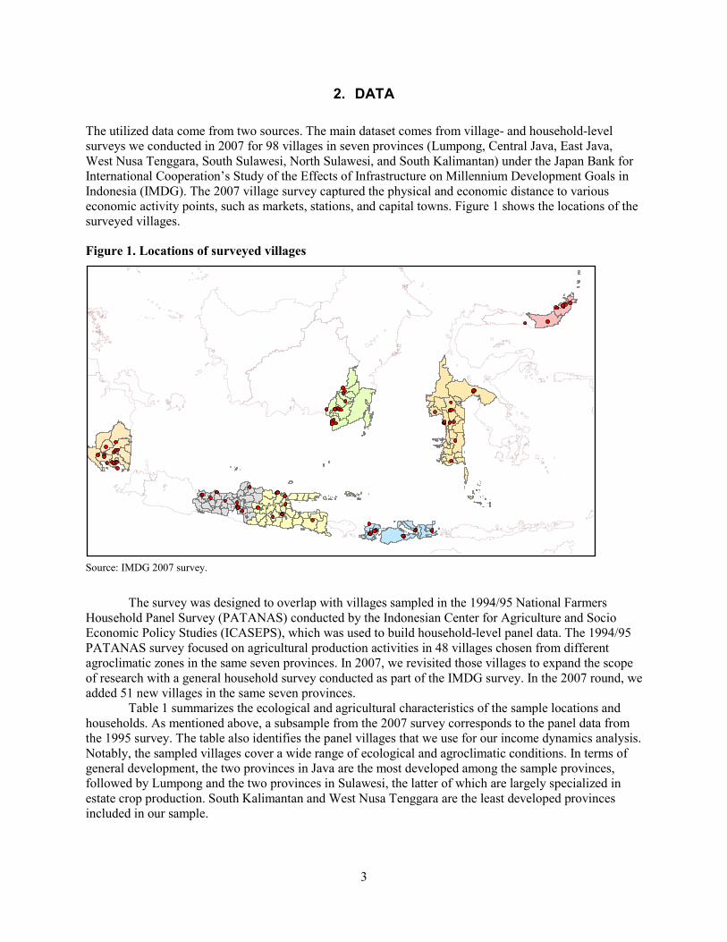
The utilized data come from two sources. The main dataset comes from village- and household-level surveys we conducted in 2007 for 98 villages in seven provinces (Lumpong, Central Java, East Java, West Nusa Tenggara, South Sulawesi, North Sulawesi, and South Kalimantan) under the Japan Bank for International Cooperation’s Study of the Effects of Infrastructure on Millennium Development Goals in Indonesia (IMDG). The 2007 village survey captured the physical and economic distance to various economic activity points, such as markets, stations, and capital towns. Figure 1 shows the locations of the surveyed villages.

Figure 1. Locations of surveyed villages

Source: IMDG 2007 survey.

The survey was designed to overlap with villages sampled in the 1994/95 National Farmers Household Panel Survey (PATANAS) conducted by the Indonesian Center for Agriculture and Socio Economic Policy Studies (ICASEPS), which was used to build household-level panel data. The 1994/95 PATANAS survey focused on agricultural production activities in 48 villages chosen from different agroclimatic zones in the same seven provinces. In 2007, we revisited those villages to expand the scope of research with a general household survey conducted as part of the IMDG survey. In the 2007 round, we added 51 new villages in the same seven provinces.

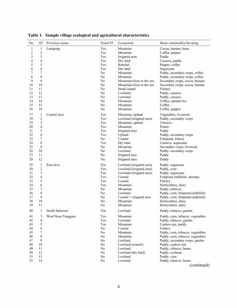
Table 1 summarizes the ecological and agricultural characteristics of the sample locations and households. As mentioned above, a subsample from the 2007 survey corresponds to the panel data from the 1995 survey. The table also identifies the panel villages that we use for our income dynamics analysis. Notably, the sampled villages cover a wide range of ecological and agroclimatic conditions. In terms of general development, the two provinces in Java are the most developed among the sample provinces, followed by Lumpong and the two provinces in Sulawesi, the latter of which are largely specialized in estate crop production. South Kalimantan and West Nusa Tenggara are the least developed provinces included in our sample.

4

Table 1. Sample village ecological and agricultural characteristics

No. ID Province name Panel 95 Ecosystem Main commodity/farming 1 1 Lampung Yes Mountain Cocoa, banana, bean 2 2 Yes Mountain Coffee, pepper 3 3 Yes Irrigated area Paddy 4 4 Yes Dry land Cassava, paddy 5 5 Yes Rainfed Pepper, coffee 6 6 Yes Dry land Sugarcane 7 7 No Mountain Paddy, secondary crops, coffee 8 8 No Mountain Paddy, secondary crops, coffee 9 9 No Mountain/close to the sea Secondary crops, cocoa, banana

10 10 No Mountain/close to the sea Secondary crops, cocoa, banana 11 11 No Small island Fishery 12 12 No Lowland Paddy, cassava 13 13 No Lowland Paddy, cassava 14 14 No Mountain Coffee, upland rice 15 15 No Mountain Coffee 16 16 No Mountain Coffee, pepper 17 1 Central Java Yes Mountain, upland Vegetables, livestock 18 2 Yes Lowland (irrigated area) Paddy, secondary crops 19 3 Yes Mountain, upland Tobacco 20 4 Yes Mountain Potato 21 5 Yes Irrigated area Paddy 22 6 Yes Upland Paddy, secondary crops 23 7 No Coastal Fishpond, fishery 24 8 Yes Dry land Cassava, sugarcane 25 9 No Mountain Secondary crops, livestock 26 10 No Lowland Paddy, secondary crops 27 11 No Irrigated area Paddy 28 12 No Irrigated area Paddy 29 1 East Java Yes Lowland (irrigated area) Paddy, sugarcane 30 2 Yes Lowland (irrigated area) Paddy, corn 31 3 Yes Lowland (irrigated area) Paddy, sugarcane 32 4 Yes Coastal Fishpond (milkfish, shrimp) 33 5 Yes Coastal Fishery 34 6 Yes Mountain Horticulture, dairy 35 7 No Mountain Paddy, tobacco 36 8 No Lowland Paddy, corn, fishpond (milkfish) 37 9 No Coastal + irrigated area Paddy, corn, fishpond (milkfish) 38 10 No Mountain Horticulture, dairy 39 11 No Mountain Horticulture, dairy 40 1 North Sulawesi Yes Lowland Paddy, tobacco, garden 41 3 West Nusa Tenggara Yes Mountain Paddy, corn, tobacco, vegetables 42 4 Yes Lowland Paddy, tobacco, garden 43 5 Yes Mountain Cashew nut, paddy 44 6 No Coastal Fishery 45 7 No Mountain Paddy, corn, tobacco, vegetables 46 8 No Mountain Paddy, corn, tobacco, vegetables 47 9 No Lowland Paddy, secondary crops, garden 48 10 No Lowland (coastal) Paddy, cashew nut 49 11 No Lowland Paddy, tobacco, beans 50 12 No Lowland (dry land) Paddy, soybean 51 13 No Lowland Paddy, corn 52 14 No Lowland Paddy, tobacco, beans

(continued)

5

Table 1 (continued) No. ID Province name Panel 95 Ecosystem Main commodity/farming 53 1 South Kalimantan No Tidal/swamp area Local paddy 54 2 No Estate plantation Rubber 55 3 No Tidal Paddy, coconut 56 4 No Tidal/swamp area Local paddy 57 5 No Tidal/swamp area Local paddy 58 6 No Coastal Fishery, paddy 59 7 No Mountain Paddy, horticulture 60 8 No Estate plantation Rubber 61 9 No Estate plantation Rubber 62 10 No Tidal/swamp area Local paddy 63 11 No Coastal Fishery, paddy 64 12 No Lowland Paddy, secondary crops 65 13 No Mountain Paddy, corn 66 14 No Tidal/swamp area Local paddy 67 15 No Tidal Coconut palm 68 16 No Tidal/swamp area Local paddy 69 1 North Sulawesi Yes Mountain Coconut, clove, paddy 70 2 Yes Irrigated area + plantation Paddy, clove, coconut 71 3 Yes Upland Horticulture 72 4 Yes Plain, rainfed Coconut, nutmeg 73 5 Yes Lowland Paddy, coconut 74 6 No Coastal Fishery 75 7 No Mountain Paddy, coconut 76 8 No Coastal-irrigated area Coconut, paddy, secondary crops 77 9 No Coastal-irrigated area Coconut, paddy, secondary crops 78 10 No Mountain Coconut, vanilla, clove, woods 79 11 No Mountain Coconut, corn, native palm 80 12 No Mountain Coconut, cocoa 81 1 South Sulawesi Yes Lowland Paddy, cocoa, coconut 82 2 Yes Irrigated area Paddy 83 3 No Irrigated area Paddy 84 4 Yes Irrigated area Paddy 85 5 Yes Mountain Coffee 86 6 Yes Mountain (dry land) Upland rice, corn 87 7 Yes Dry land, plantation Cocoa 88 8 No Lowland (coastal) Paddy, fishpond 89 9 No Lowland (coastal) Paddy, fishpond 90 10 No Lowland (coastal) Paddy, fishpond 91 11 No Irrigated area Paddy 92 12 No Irrigated area Paddy 93 13 No Coastal Fishery, fishpond 94 14 No Lowland Paddy, cocoa, coconut 95 15 No Lowland Paddy, cocoa, coconut 96 16 No Lowland Paddy, cocoa, coconut 97 17 No Irrigated land and fishpond Paddy, milkfish 98 18 No Coastal Milkfish, shrimp

Note: No. 2 of West Nusa Tenggarra was dropped due to the fact that access to the village was unsafe in 2007, and we added a new village in the province.

In the revisited villages, we resampled 20 households per village from the 1994/95 sample and followed the split households. In the newly surveyed villages, we sampled 24 households from two main hamlets in each village. Since one of the 48 villages included in the 1994/95 PATANAS (in West Nusa Tenggara Province) was not accessible in 2007 for safety reasons, our final sample includes data from a total of 98 villages. For the panel analysis, we construct a household income panel using data from 34

6

villages in six provinces (Lumpong, Central Java, East Java, West Nusa Tenggara, South Sulawesi, and North Sulawesi) for which we had 2007 household and 1994/95 PATANAS survey data.4

Additional data come from the 1996 and 2006 Village Potential Statistics (PODES), which is a village census conducted by the Republic of Indonesia Central Bureau of Statistics (described in detail in Section 3).

4 The 1994/95 PATANAS survey consists of two sub-surveys. The income and production data used herein are drawn from

the second part, which contains information from 34 villages in six provinces (excluding South Kalimantan). To merge the household panel data with the spatial data on road quality from PODES 1996 and 2006, we interact subdistrict and district-level road quality variables with household- and village-level variables such as land owned and distance to a district center. We cannot construct road quality datasets for two of the subdistricts in North Sulawesi, which are not fully captured in PODES. When we previously constructed village panel data from PODES for other studies aimed at analyzing village dynamics, we had problems linking villages across rounds due to village divisions and mergers associated (at least in part) with the country’s decentralization. To solve this problem, we linked the subdistricts and then linked the villages within each subdistrict by their names. In the present study, however, this is less of an issue because we use only subdistrict-level information (the average proportion of asphalt roads among the intervillage roads).

7

3. DESCRIPTIVE ANALYSES

Spatial Connectivity

Intervillage Road Improvement

In this section, we describe the village census and PODES data with an emphasis on transportation, road quality variables, and changes in local road quality from 1996 to 2006. The data cover all villages in the census years. We use the 1996 and 2006 rounds because our household panel data come from 1995 and 2007. In the panel analysis, we take the difference between 1996 and 2006 to represent changes in the average local road quality during the study period.

The PODES data include information on major intervillage traffic. If the major traffic is on land, the data include information regarding the type of widest road for land transport (for example, asphalt, concrete, cone-block, hardened, soil, and others), and whether four-wheel or more vehicles can pass the road all year long. From the above information, it is possible to construct indicator variables for the following: (1) whether the major intervillage traffic is by land or not; (2) whether the widest road is asphalt, concrete, cone-block, or not; (3) whether the widest road is hardened or not; (4) whether the widest road is soil or not; (5) whether the widest road is “other” or not; and (6) whether vehicles with four or more wheels can pass the road all year long or not.

For the present study, we use measure (2) to capture transportation speed in the local economy. The average is taken at the subdistrict, district, and provincial levels for each round as

where is an indicator variable that takes the value of one if the majority of intervillage traffic is on land and the road is constructed of asphalt/concrete/cone-block (good quality), or zero otherwise (bad quality), N(j) is a set of villages within the neighborhood of village j, and #N(j) is the number of villages in N(j). Therefore, zt(j) is the probability of village j having good-quality transportation in its neighborhood, which is assumed to be positively correlated with the average transportation speed in the local economy.

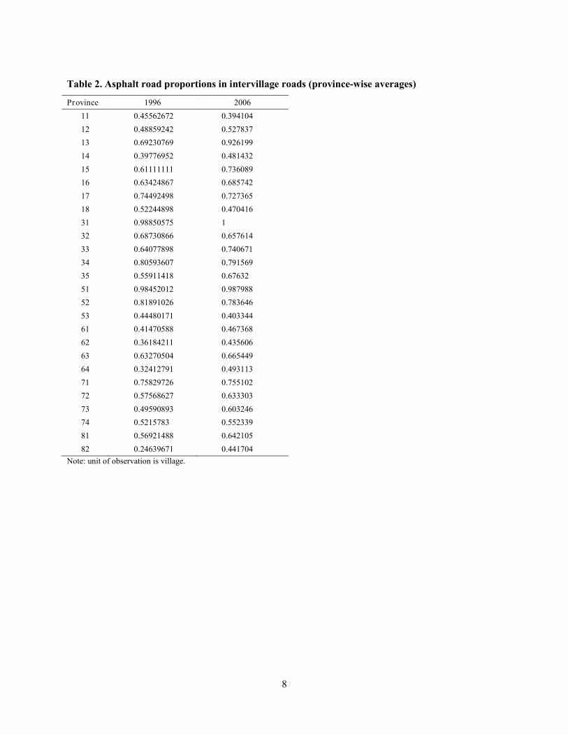
Table 2 shows the province-level averages of asphalt road indicators in 1996 and 2006. To make the data from the two years comparable, we use the 1996 provinces for villages that experienced changes in their province/district classifications between 1996 and 2006. This comparison reveals that there are interprovincial disparities in average road quality for both years, and also that the average proportion of asphalt intervillage roads improves over time in many provinces.

Table 3 shows village-level changes in intervillage road quality (asphalt or not) between 1996 and 2007. In many provinces, a higher proportion of villages show intervillage road quality improvement versus deterioration. However, a large number of villages show no change in quality, and a nonnegligible number of villages show deterioration of road quality. The reasons underlying the deterioration of road quality are not obvious from the data, but may be related to inadequate road maintenance or construction of new, poor quality roads.

Next, we take the difference between the two rounds to examine the improvement or deterioration of road quality in the local economies as follows:

Interestingly, we find that the changes in all regions are symmetrically distributed with either improvement or deterioration, although the majority of cases show relatively small changes around zero (see Figure 2).

8

Table 2. Asphalt road proportions in intervillage roads (province-wise averages)

Province 1996 2006 11 0.45562672 0.394104 12 0.48859242 0.527837 13 0.69230769 0.926199 14 0.39776952 0.481432 15 0.61111111 0.736089 16 0.63424867 0.685742 17 0.74492498 0.727365 18 0.52244898 0.470416 31 0.98850575 1 32 0.68730866 0.657614 33 0.64077898 0.740671 34 0.80593607 0.791569 35 0.55911418 0.67632 51 0.98452012 0.987988 52 0.81891026 0.783646 53 0.44480171 0.403344 61 0.41470588 0.467368 62 0.36184211 0.435606 63 0.63270504 0.665449 64 0.32412791 0.493113 71 0.75829726 0.755102 72 0.57568627 0.633303 73 0.49590893 0.603246 74 0.5215783 0.552339 81 0.56921488 0.642105 82 0.24639671 0.441704

Note: unit of observation is village.

9

Table 3. Village-level changes in intervillage road quality (asphalt/concrete/cone-block or not), 1996–2006

Province name

Number of villages Propor tion of villages in each province No change

Deter iorated Improved Total

No change

Deter iorated Improved

Difference (improved)-

(deter iorated) Remain good Remain bad Remain good Remain bad (percent) Jawa Barat 516 546 230 128 1,420 36.3 38.5 16.2 9.0 -7.2 Lampung 373 60 53 35 521 71.6 11.5 10.2 6.7 -3.5 Maluku 249 349 91 70 759 32.8 46.0 12.0 9.2 -2.8 Jambi 586 154 101 77 918 63.8 16.8 11.0 8.4 -2.6 South Kalimantan 303 47 42 35 427 71.0 11.0 9.8 8.2 -1.6 East Java 1,067 438 279 250 2,034 52.5 21.5 13.7 12.3 -1.4 Aceh 989 1,907 689 649 4,234 23.4 45.0 16.3 15.3 -0.9 Kalimantan Timur 602 3 8 10 623 96.6 0.5 1.3 1.6 0.3 Bali 1,277 1,277 385 424 3,363 38.0 38.0 11.4 12.6 1.2 Sulawesi Tengah 349 125 71 82 627 55.7 19.9 11.3 13.1 1.8 Central Java 258 0 0 7 265 97.4 0.0 0.0 2.6 2.6 Riau 860 599 139 189 1,787 48.1 33.5 7.8 10.6 2.8 West Nusa Tenggara 188 378 56 78 700 26.9 54.0 8.0 11.1 3.1 Sumatra Barat 261 207 56 78 602 43.4 34.4 9.3 13.0 3.7 Sumatra Selatan 190 357 12 36 595 31.9 60.0 2.0 6.1 4.0 Irian Jaya 1,162 646 157 261 2,226 52.2 29.0 7.1 11.7 4.7 Nusa Tenggara Timur 101 759 25 81 966 10.5 78.6 2.6 8.4 5.8 North Sulawesi 968 695 179 314 2,156 44.9 32.2 8.3 14.6 6.3 Sumatera Utra 152 251 17 49 469 32.4 53.5 3.6 10.4 6.8 Bengkulu 215 37 8 28 288 74.7 12.8 2.8 9.7 6.9 Sulawesi Tenggara 561 423 73 159 1,216 46.1 34.8 6.0 13.1 7.1 South Sulawesi 139 502 18 73 732 19.0 68.6 2.5 10.0 7.5 DKI Jakarta 378 137 64 123 702 53.8 19.5 9.1 17.5 8.4 Kalimantan Barat 4,379 1,361 684 1,441 7,865 55.7 17.3 8.7 18.3 9.6 DI Yogyakarta 268 536 61 171 1,036 25.9 51.7 5.9 16.5 10.6 Kalimantan Tengah 3,653 1,756 807 1,746 7,962 45.9 22.1 10.1 21.9 11.8

Total 20,044 13,550 4,305 6,594 44,493 45.0 30.5 9.7 14.8 5.1

10

Figure 2. Changes in average intervillage road quality (asphalt road proportion)

Notes: X-axis: Changes in subdistrict level average road quality. Y-axis: Frequency. Regional groups: 1, Sumatra; 2, Java (excluding Jakarta); 3, Kalimantan; 4, Sulawesi; 5, others (excluding Bali).

At the subdistrict level, improvement and deterioration coexist over the ten-year study period, allowing us to examine the impact of intervillage road quality changes on household income dynamics. Comparison of road quality changes (at the subdistrict level) between Java and non-Javan regions showed that Javan areas experience a faster improvement compared to regions outside Java.

Distance to Economic Centers

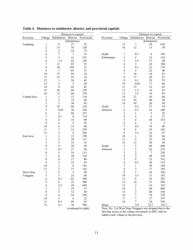
We assume that the physical distances between each village and its economic center are constant throughout the period, so these distances are taken as predetermined. This is important, because we hypothesize that spatial connectivity development has uneven impacts on village economies, depending on each village’s distance to the main economic activity points. Table 4 shows the distances to the centers of all 98 sampled villages, as observed from the 2007 village survey.

11

Table 4. Distances to subdistrict, district, and provincial capitals Distance to capital Distance to capital Province Village Subdistr ict Distr ict Provincial Province Village Subdistr ict Distr ict Provincial (kilometers) (kilometers) Lampung 1 9 37 53 13 7 49 650 2 13 56 120 14 12 13 39 3 5 14 75 4 7 7 67 South

Kalimantan 1 0.5 4 102

5 3 15 125 2 4 12 124 6 3.5 42 145 3 3.5 37 40 7 12 85 55 4 3 10 180 8 38 104 12 5 0.1 22 170 9 7 85 37 6 4 22 90 10 37 95 14 7 18 18 61 11 35 95 14 8 17 20 67 12 1 10 45 9 0.1 29 79 13 5 5 50 10 0.05 17 86 14 4 45 82 11 15 32 45 15 20 80 120 12 1.5 16 81 16 15 60 150 13 3.5 10 93 Central Java 1 3 13 110 14 21 45 60 2 3 15 50 15 50 40 50 3 3 30 93 16 50 20 50 4 10 60 120 North

Sulawesi 1 0.3 27 54

5 0.05 30 250 2 0.7 18 100 6 2 60 225 3 1 5 25 7 0.1 8 114 4 4 6 27 8 4 14 90 5 4 40 335 9 6 5 93 6 6 5 5 10 6 15 60 7 0.5 18 60 11 7 15 270 8 6 25 105 12 5 8 250 9 3.5 16 97 East Java 1 3 15 190 10 1 30 60 2 5 20 137 11 4 23 59 3 5 14 35 12 13 20 50 4 4 20 38 South

Sulawesi 1 3 60 600

5 0.7 27 90 2 5 42 279 6 5 14 115 3 2 7 258 7 6 20 218 4 3 48 126 8 4 17 80 5 9 33 352 9 2 25 93 6 0.5 28 114 10 1 8 145 7 1 30 140 11 2 27 145 8 3 17 189 West Nusa Tenggara

1 5 5 50 9 3 16 186 3 5 25 60 10 3.5 13 183

4 0.1 62 300 11 8 45 282 5 6 25 500 12 16 51 280 6 2.5 44 640 13 2 16 185 7 2 19 57 14 1 60 600 8 5 12 50 15 2 60 530 9 8 54 250 16 7 70 570 10 3 4 22 17 7 17 197 11 0.3 44 45 18 7 24 250 12 0.1 30 500 Mean 6.9 32.7 141.1 (continued to right) Note: No. 2 of West Nusa Tenggara was dropped due to the

fact that access to the village was unsafe in 2007, and we added a new village in the province.

12

Household Income In the analysis of household income dynamics, we use household panel data collected from six provinces during the 1995 and 2007 survey rounds. Both surveys include detailed information on income-generating activities. For the present study, we aggregate the incomes from these activities to construct household-level income measures. Some 2007 households had split from the 1995 households (called original households), so we aggregate incomes from both original and split households in 2007 to allow comparison with the 1995 original households. When we aggregate incomes from original and split households in 2007 using the 1995 household units, the results are quite similar, implying that the attrition (split) bias in our panel analysis is not large.

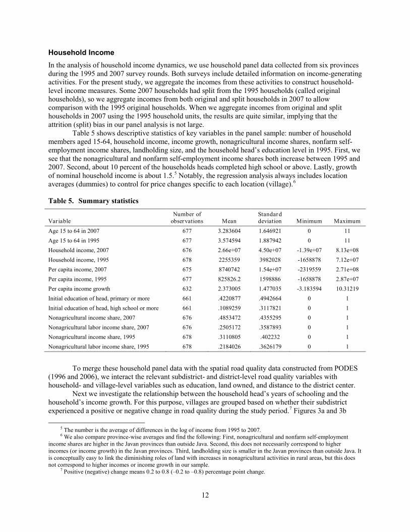
Table 5 shows descriptive statistics of key variables in the panel sample: number of household members aged 15-64, household income, income growth, nonagricultural income shares, nonfarm self-employment income shares, landholding size, and the household head’s education level in 1995. First, we see that the nonagricultural and nonfarm self-employment income shares both increase between 1995 and 2007. Second, about 10 percent of the households heads completed high school or above. Lastly, growth of nominal household income is about 1.5.5 Notably, the regression analysis always includes location averages (dummies) to control for price changes specific to each location (village).6

Table 5. Summary statistics

Var iable Number of

observations Mean Standard deviation Minimum Maximum

Age 15 to 64 in 2007 677 3.283604 1.646921 0 11 Age 15 to 64 in 1995 677 3.574594 1.887942 0 11 Household income, 2007 676 2.66e+07 4.50e+07 -1.39e+07 8.13e+08 Household income, 1995 678 2255359 3982028 -1658878 7.12e+07 Per capita income, 2007 675 8740742 1.54e+07 -2319559 2.71e+08 Per capita income, 1995 677 825826.2 1598886 -1658878 2.87e+07 Per capita income growth 632 2.373005 1.477035 -3.183594 10.31219 Initial education of head, primary or more 661 .4220877 .4942664 0 1 Initial education of head, high school or more 661 .1089259 .3117821 0 1 Nonagricultural income share, 2007 676 .4853472 .4355295 0 1 Nonagricultural labor income share, 2007 676 .2505172 .3587893 0 1 Nonagricultural income share, 1995 678 .3110805 .402232 0 1 Nonagricultural labor income share, 1995 678 .2184026 .3626179 0 1

To merge these household panel data with the spatial road quality data constructed from PODES (1996 and 2006), we interact the relevant subdistrict- and district-level road quality variables with household- and village-level variables such as education, land owned, and distance to the district center.

Next we investigate the relationship between the household head’s years of schooling and the household’s income growth. For this purpose, villages are grouped based on whether their subdistrict experienced a positive or negative change in road quality during the study period.7

5 The number is the average of differences in the log of income from 1995 to 2007.

Figures 3a and 3b

6 We also compare province-wise averages and find the following: First, nonagricultural and nonfarm self-employment income shares are higher in the Javan provinces than outside Java. Second, this does not necessarily correspond to higher incomes (or income growth) in the Javan provinces. Third, landholding size is smaller in the Javan provinces than outside Java. It is conceptually easy to link the diminishing roles of land with increases in nonagricultural activities in rural areas, but this does not correspond to higher incomes or income growth in our sample.

7 Positive (negative) change means 0.2 to 0.8 (–0.2 to –0.8) percentage point change.

13

show per capita income growth in villages located in subdistricts that experienced positive (negative) changes in road quality. Income growth is demeaned by village effects, so we observe intra-village variations using the residuals. Interestingly, when the road quality improves, income growth is relatively constant among households with heads educated up to completion of junior high school, but this income growth substantially increases among households with heads that completed senior high school and above. This indicates that there may be a threshold schooling level, beyond which local road quality changes and education jointly increase income growth. In villages that experienced deterioration of road quality, the negative impact on income growth is larger among educated households.

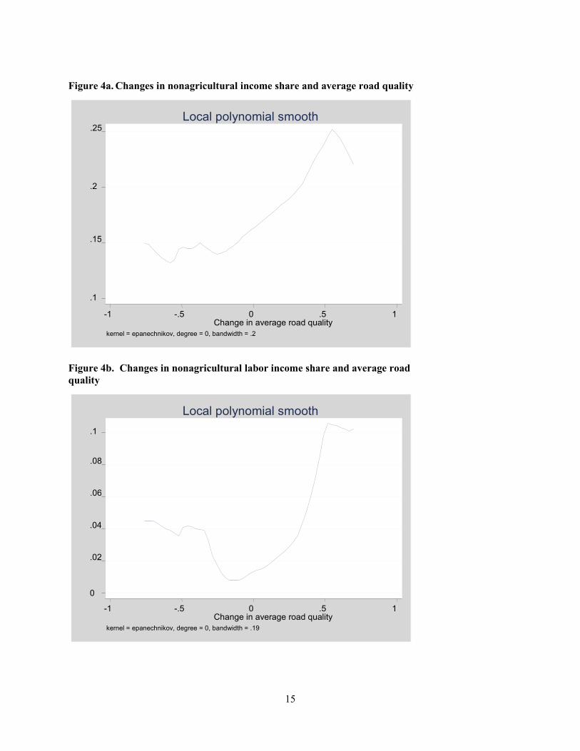
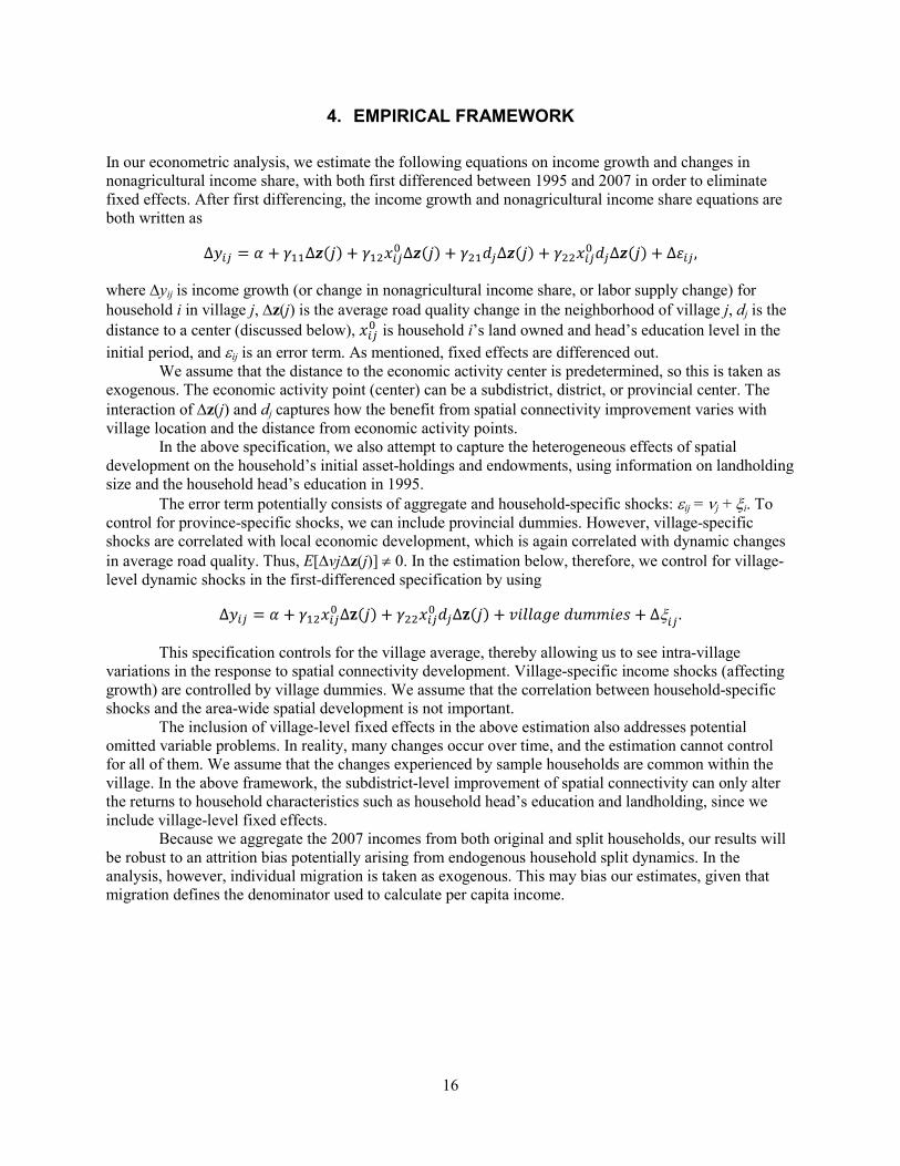
Figures 4a and 4b, which show the relationship between changes in average road quality and nonagricultural income share, reveal that the improvement of intervillage roads within a subdistrict is associated with an increase in the nonagricultural income share. This is particularly strong for nonagricultural labor income. Our econometric analysis confirms this observation.

14

Figure 3a. Per capita income growth and household head’s education under conditions of improved road quality

Figure 3b. Per capita income growth and household head’s education under conditions of deteriorated road quality

-.3

-.2

-.1

0

.1

0 5 10 15 yrschool

kernel = epanechnikov, degree = 0, bandwidth = 1.69

Local polynomial smooth

15

Figure 4a. Changes in nonagricultural income share and average road quality

Figure 4b. Changes in nonagricultural labor income share and average road quality

0

.02

.04

.06

.08

.1

-1 -.5 0 .5 1 Change in average road quality

kernel = epanechnikov, degree = 0, bandwidth = .19

Local polynomial smooth

.1

.15

.2

.25

-1 -.5 0 .5 1 Change in average road quality

kernel = epanechnikov, degree = 0, bandwidth = .2

Local polynomial smooth

16

4. EMPIRICAL FRAMEWORK

In our econometric analysis, we estimate the following equations on income growth and changes in nonagricultural income share, with both first differenced between 1995 and 2007 in order to eliminate fixed effects. After first differencing, the income growth and nonagricultural income share equations are both written as

where ∆yij is income growth (or change in nonagricultural income share, or labor supply change) for household i in village j, ∆z(j) is the average road quality change in the neighborhood of village j, dj is the distance to a center (discussed below), is household i’s land owned and head’s education level in the initial period, and εij is an error term. As mentioned, fixed effects are differenced out.

We assume that the distance to the economic activity center is predetermined, so this is taken as exogenous. The economic activity point (center) can be a subdistrict, district, or provincial center. The interaction of ∆z(j) and dj captures how the benefit from spatial connectivity improvement varies with village location and the distance from economic activity points.

In the above specification, we also attempt to capture the heterogeneous effects of spatial development on the household’s initial asset-holdings and endowments, using information on landholding size and the household head’s education in 1995.

The error term potentially consists of aggregate and household-specific shocks: εij = νj + ξi. To control for province-specific shocks, we can include provincial dummies. However, village-specific shocks are correlated with local economic development, which is again correlated with dynamic changes in average road quality. Thus, E[∆vj∆z(j)] ≠ 0. In the estimation below, therefore, we control for village-level dynamic shocks in the first-differenced specification by using

This specification controls for the village average, thereby allowing us to see intra-village variations in the response to spatial connectivity development. Village-specific income shocks (affecting growth) are controlled by village dummies. We assume that the correlation between household-specific shocks and the area-wide spatial development is not important.

The inclusion of village-level fixed effects in the above estimation also addresses potential omitted variable problems. In reality, many changes occur over time, and the estimation cannot control for all of them. We assume that the changes experienced by sample households are common within the village. In the above framework, the subdistrict-level improvement of spatial connectivity can only alter the returns to household characteristics such as household head’s education and landholding, since we include village-level fixed effects.

Because we aggregate the 2007 incomes from both original and split households, our results will be robust to an attrition bias potentially arising from endogenous household split dynamics. In the analysis, however, individual migration is taken as exogenous. This may bias our estimates, given that migration defines the denominator used to calculate per capita income.

17

5. EMPIRICAL RESULTS

Income Growth and Nonagricultural Share In this section, we summarize the main results from our household analysis, which examines household income growth and changes in nonagricultural income share. Preliminary analyses show that subdistrict-level road quality measures explain income growth and changes in nonagricultural income share better than district- and province-level road quality measures, probably due to subdistrict-level variations in the sample and the fact that localized spatial connectivity development opens access to wider economic activities (such as district and provincial centers). Based on preliminary analysis, we decide to restrict the sample to those with changes in the asphalt road proportion that are in the range of minus 0.3 to 0.8. Extreme values outside the range create large noise in the estimation.8

To capture the potentially heterogeneous effects of the subdistrict average road quality improvement on income growth, we introduce some heterogeneity into the analysis by including household head’s education level in 1995 (at the household level) and the distances to subdistrict, district, and provincial centers (at the village level).

9

Here, the main analytical point is to investigate the role of post-primary education in income growth when spatial connectivity is improving in the local neighborhood and from there to investigate the relationship with connectivity to larger, more distant economic centers.

10

In Table 6, Column 1 shows the results when we use an indicator that takes the value of one if the household head has completed high school or higher, and zero otherwise, and interact this indicator with the 1995 intervillage road quality indicator and the distances to the subdistrict, district, and provincial centers. First, the initial level of household education significantly increases income growth. Second, our results support complementarity between education and road quality, the educated benefit from improvement in road quality in neighborhood economy. Third, we also find that the distance factors do significantly affect the education-spatial network effects on per capita income growth.

We include village dummies to control for village-specific shocks and corresponding price changes specific to the village economy.

In Columns 2 and 3, we examine changes in nonagricultural total income share and nonagricultural labor income share, respectively. The results are comparable. First, the education effect is insignificant in both cases. Second, the distance to the subdistrict capital significantly increases the marginal effect of education on nonagricultural total income share. Third, and more interesting, the change in nonagricultural labor income share increases marginally significantly with the distance from the provincial capital. The above findings may imply that the impact of improved local spatial networks on the transition to nonagricultural income sources (especially labor income) tends to be positive in remote villages.

8 Similarly, our estimation excludes two observations that show income growth as too large. 9 In our empirical setting with a small number of villages in each subdistrict, we cannot identify the effect of subdistrict-

level road quality changes on household-level outcomes. Therefore, we focus on intra-village distributional effects (with village dummies controlling for price changes and village-level shocks) in our parametric estimation.

10 Education level can change over time, creating an endogeneity issue. Changes in household income and spatial connectivity can affect changes in the household education level. Statistically, the first differencing and the inclusion of village-level fixed effects mitigate the above endogeneity problem, since we are only concerned with the correlation between household-specific shocks and the initial level of household schooling. However, we should consider the direction of the potential bias. Dewina and Yamauchi (2009) show that intergenerational educational growth in the same dataset, as measured by the gap between household head’s education and the maximum level of educational attainment in the household in 1995, significantly explains income growth. Yamauchi (2009) also demonstrates significant changes in educational attainment in Indonesia in the 1970s and 1980s. These findings suggest that a higher level of schooling attainment by the household head implies, on average, a lower education gap with the maximum level of educational attainment in the household. If so, the potential bias in the education effect is small. However, if a higher level of educational attainment by the head means higher growth of educational attainment within the household, we may face a potentially large upward bias.

18

Table 6. Changes in nonagricultural income (1) (2) (3) (4)

Dependent

Per capita income growth

Change in nonagr icultural

income share

Change in nonagr icultural

labor income share

Per capita nonagr icultural

labor income growth

High school or higher 0.6406 0.0418 0.0852 2.572 (2.31) (0.49) (1.11) (2.97)

Change in average road quality × high school or higher 7.266 -0.5774 0.2734 8.415

(3.64) (1.08) (0.46) (1.11)

× High school × asphalt in 1995 -1.594 0.1348 -0.2753 -3.502

(1.32) (0.39) (0.87) (0.96)

× High school × distance to subdistrict capital 0.1381 0.0687 0.0683 0.5910

(2.90) (4.24) (3.78) (3.14)

× High school × distance to district capital -0.4981 -0.0153 -0.0668 -1.359

(3.31) (0.35) (1.40) (2.55)

× High school × distance to provincial capital 0.0398 0.0014 0.0070 0.1254

(3.58) (0.42) (1.71) (2.87) Village dummies Yes Yes Yes Yes R-squared 0.1634 0.1195 0.1189 0.1066 Number of observations 540 540 540 540 Notes: numbers in parentheses are absolute t-values, which we calculate using robust standard errors with village-level clusters. In column 4, we assign 1,000 rupiah to zero values in order to compute income growth.

In Column 4, we attempt to directly verify the above conjecture, by using the growth of nonagricultural labor income from 1995 to 2007. For this analysis, incomes of zero are assigned a value of 1,000 rupiah, allowing us to compute income growth. First, the direct effect of education is insignificantly positive. Second, complementarity between education and spatial network becomes insignificant. However, third, location factors, measured by distances from economic centers, significantly alter the complementarity of the distance factors. The distance from the provincial capital significantly increases nonagricultural labor income growth if the household head has attained a high school or higher education and the neighboring road networks improve over time. These findings are consistent with those shown in Figures 3 and 4.

The marginal benefits from local road quality improvement are large in remote areas, probably because there is a low level of capital accumulation. However, our results show that the district center is always important to the local economy, given localized economic interactions at the district level. There seem to be two important dimensions to this economic connectivity: links to the local economy (district capital), and links to the larger economic demand center (provincial capital). In the former, proximity to the center is always beneficial for the educated. However, areas far from the latter (that is, districts far from the provincial capital) are more likely to benefit from local road quality improvement. Regardless of interactions with distance, however, education always increases the marginal benefits from local road quality improvement.

In our definition, nonagricultural activities only cover those undertaken by current household members, excluding nonmembers who work/live at a distance from their original villages (that is, those

19

who do not commute). Therefore, we may be missing migration-linked, nonagricultural transitions.11

In the estimation, we include clustered correlations within the village in order to compute robust standard errors. There may be correlations across shocks outside the village (even after village-level fixed effects are used to control for village-specific shocks), such as when income shocks are positively correlated within a province. In our preliminary analysis, we experimented with district- and province-level clusters, and the results proved the robustness of our results. However, we do not explicitly incorporate any correlation structure that decays with physical or economic distance.

Instead, income growth (as defined herein) includes agriculture-based growth, such as that arising from improved marketing of agricultural products (for example, vegetables). In this activity, connecting to larger demand centers seems to be a driving force.

Labor Supply to the Nonagricultural Sector This section focuses on the household behavior of labor supply to the non-agricultural sector. In the previous section, we show that income growth does not necessarily match the share change of nonagricultural income sources. To resolve this issue, we next examine nonagricultural labor market behavior.

We construct the share of labor supplied to nonagricultural activities in 1995 and 2007. The number of household members aged 15 to 64 defines the household labor endowment (converted to man-days, assuming that each individual works 250 days a year). Since we note that the 1995 survey undercounted household members, we use the 1995 member list reconstructed from the 2007 survey. For actual man-days worked in nonagricultural activities, we use data from the 1995 and 2007 surveys. For our analysis of labor supply dynamics, we use the change in the share of labor supplied to nonagricultural activities.12

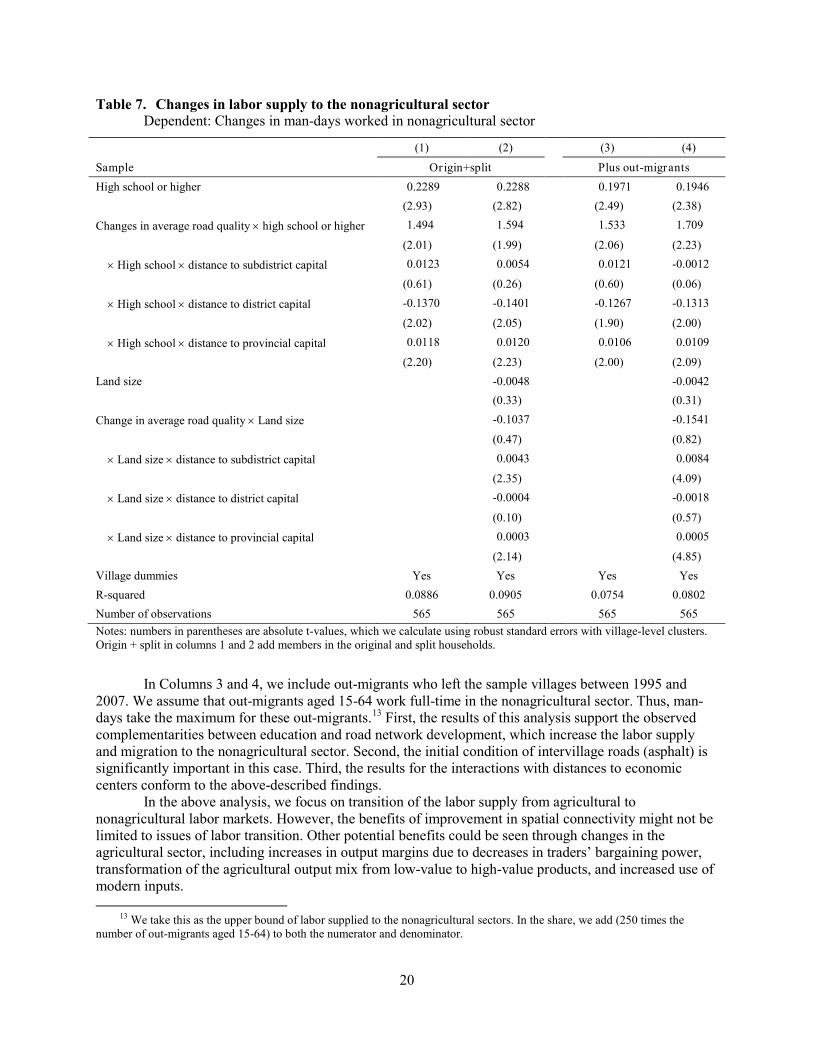
Table 7 shows the change in man-days worked in the nonagricultural labor market from 1995 to 2007. Columns 1 and 2 use the sample of household members in the original and split households living in the sample villages in 2007.

The results reveal that the signs and significance of the parameter estimates are quite similar to those of the income growth equations shown in Table 6. Educational attainment at the secondary or higher level helps households gain more from spatial network development. Complementarity between education and local road quality is significant. In remote villages (that is, those distant from the provincial capital), the gain is large. The direct role of initial landholding is not significant, but location factors play a similar role, that is, distance from provincial capital augments the complementarity with spatial network.

11 We see a negative effect of schooling on the change in nonagricultural income share (through the interaction term with

changes in road quality). First, those who are educated at the initial stage are more likely than the less educated to have nonagricultural income opportunities; therefore, local road quality improvement has a smaller marginal effect on the transition of the educated to the nonagricultural sector. Second, more educated households also have more assets for agricultural production; thus road quality improvement increases the productivity of their farm activities more significantly. Third, individual-level selectivity may account for the above result. At the individual level, the educated are more likely to move out of households over time, in order to pursue higher income opportunities in nonagricultural sectors. The comparison of completed schooling between current household members and nonmembers shows that there is higher average schooling among nonmembers. In households with educated heads, other members are also more likely to be educated. If such migration selection is important during the period of 1995-2007, there may be an inverse correlation between schooling (at the household level) and observed nonagricultural transitions. This is because educated agents tend to leave, while relatively less educated household members tend to stay.

12 Some individuals may work more than 250 days per year. It is also possible that household members younger than 15 or older than 65 could work in nonagricultural sectors (although it is illegal for children under 15 to work). In some households, our roster may miss some members who contribute to the household income; however, their labor supply and incomes are captured. For all these possible reasons, the estimated share of labor can be above one. In this case, we adjust the values to one. In the present analysis, however, we take the difference between 1995 and 2007, which minimizes this potential problem.

20

Table 7. Changes in labor supply to the nonagricultural sector Dependent: Changes in man-days worked in nonagricultural sector (1) (2) (3) (4)

Sample Or igin+split Plus out-migrants High school or higher 0.2289 0.2288 0.1971 0.1946 (2.93) (2.82) (2.49) (2.38)

Changes in average road quality × high school or higher 1.494 1.594 1.533 1.709

(2.01) (1.99) (2.06) (2.23)

× High school × distance to subdistrict capital 0.0123 0.0054 0.0121 -0.0012

(0.61) (0.26) (0.60) (0.06)

× High school × distance to district capital -0.1370 -0.1401 -0.1267 -0.1313

(2.02) (2.05) (1.90) (2.00)

× High school × distance to provincial capital 0.0118 0.0120 0.0106 0.0109

(2.20) (2.23) (2.00) (2.09) Land size -0.0048 -0.0042 (0.33) (0.31)

Change in average road quality × Land size -0.1037 -0.1541

(0.47) (0.82)

× Land size × distance to subdistrict capital 0.0043 0.0084

(2.35) (4.09)

× Land size × distance to district capital -0.0004 -0.0018

(0.10) (0.57)

× Land size × distance to provincial capital 0.0003 0.0005

(2.14) (4.85) Village dummies Yes Yes Yes Yes R-squared 0.0886 0.0905 0.0754 0.0802 Number of observations 565 565 565 565 Notes: numbers in parentheses are absolute t-values, which we calculate using robust standard errors with village-level clusters. Origin + split in columns 1 and 2 add members in the original and split households.

In Columns 3 and 4, we include out-migrants who left the sample villages between 1995 and 2007. We assume that out-migrants aged 15-64 work full-time in the nonagricultural sector. Thus, man-days take the maximum for these out-migrants.13

In the above analysis, we focus on transition of the labor supply from agricultural to nonagricultural labor markets. However, the benefits of improvement in spatial connectivity might not be limited to issues of labor transition. Other potential benefits could be seen through changes in the agricultural sector, including increases in output margins due to decreases in traders’ bargaining power, transformation of the agricultural output mix from low-value to high-value products, and increased use of modern inputs.

First, the results of this analysis support the observed complementarities between education and road network development, which increase the labor supply and migration to the nonagricultural sector. Second, the initial condition of intervillage roads (asphalt) is significantly important in this case. Third, the results for the interactions with distances to economic centers conform to the above-described findings.

13 We take this as the upper bound of labor supplied to the nonagricultural sectors. In the share, we add (250 times the

number of out-migrants aged 15-64) to both the numerator and denominator.

21

6. POLICY DISCUSSION

Here, we seek to bridge the gap between academic studies and infrastructure planning. Previous academic studies on the spatial connectivities of rural households are limited in the sense that they perceive connectivity as either access to local towns or remoteness from growth centers, and do not discuss the combination of both. In actual policy choices, however, public investment planners face decisions on the allocation of resources among trunk roads (that lead to economic centers) and local roads. Public investment planners also face policy choices regarding the balance between spending on education and on roads.

The analyses reported herein suggest that the more educated households can increase their incomes to a higher degree, given better spatial connectivity at the local level. Better local road quality may also improve the access for remote villages to trunk roads, thus helping the more educated engage in better job/business opportunities at district capital (local economy) or provincial capital (larger economic center).

However, the effect on income growth is larger when the village is close to the district center, and/or distant from the provincial center. Although not specifically examined in our empirical analysis due to data limitations, this difference may be due to market space and/or the value-added nature of different income-generating activities. For example, some income-generating activities focus on the market, with the district capital as the local economic center. These may include activities such as food processing with low value-added (such as dried fish or chips/crackers) and marketing of staple foods. In this case, proximity to the economic center is key, as it reduces transport-related transaction costs. However, other income-generating activities have wider market areas, especially those catering to urban economic centers (for example, provincial centers). These may include higher value-added goods sold in large urban markets, such as bamboo or wood products. Another example can be high-quality vegetables for the urban market. In such a case, the added value can cover the transaction cost due to transportation; in this case, a greater distance from the provincial center is not an obstacle, provided that the household is connected to economic centers. Better road connectivity to the provincial center due to local road improvement may therefore give households in remote villages the chance to market such value-added products.

Improving the trunk roads connecting villages to closer district centers is important, but should occur alongside the improvement of local roads providing access to the trunk roads. It is also important to develop the network of trunk roads to secure connectivity to distant economic centers (for example, the provincial capital), alongside the improvement of local roads.

Poverty Reduction Strategies (PRSs) adopted by low-income countries (especially those in Africa) are currently entering a second, growth-focused stage (as compared to the previous generation of PRSs, which emphasized budget allocation to primary education and health). However, little is known on the type of public investment combinations that induce growth. The analyses herein suggest that there may be value in simultaneously investing in spatial connection of local neighborhoods plus connection to distant economic centers. Furthermore, there may be benefit in concurrently investing in both higher education (high school and above) and road development. Although actual PRSs should be country-driven and country-specific, our findings may help add value to the next generation of growth-oriented PRSs.

22

7. CONCLUSION

This paper examines the impact of spatial connectivity development on household income growth and the transition to nonagriculture, by combining household panel data and village census data from Indonesia. Our empirical results show that the impacts of improved local road quality (which positively correlates with an increase in transportation speed) on income growth and transition to nonagricultural activities depend on the distance to economic centers, household education level, and landholding size. In particular, postprimary education significantly increases the benefit of local connectivity improvement in remote areas and the transition to nonagricultural labor markets. Postprimary education and local road quality are complementary, increasing income growth and labor supply to the nonagricultural sector.

23

REFERENCES

Aschauer, D. A. 1989a. Is public expenditure productive? Journal of Monetary Economics 23 (2): 177–200.

________. 1989b. Public investment and productivity growth in the Group of Seven. Federal Reserve Bank of Chicago. Economic Perspectives 13 (5): 17–25.

Benjamin, D. 1992. Household composition, labor markets, and labor demand: Testing for separation in agricultural household models. Econometrica 60 (2): 287–322.

Binswanger, H., S. R. Khandker, and M. R. Rosenzweig. 1993. How infrastructure and financial institutions affect agricultural output and investment in India. Journal of Development Economics 41 (2): 337–366.

Dewina, R., and F. Yamauchi. 2009. Human capital, mobility, and income dynamics: Evidence from Indonesia. Japan International Cooperation Agency, Tokyo, and International Food Policy Research Institute, Washington, D.C. Photocopy.

Fafchamps, M. 1993. Sequential labor decisions under uncertainty: An estimable household model of West African farmers. Econometrica 61 (5): 1173–1198.

Fafchamps, M., and F. Shilpi. 2003. Spatial division of labor in Nepal. Journal of Development Studies 39 (6): 23–66.

________. 2005. Cities and spacialization: Evidence from South Asia. Economic Journal 115 (503): 477–504.

Fafchamps, M., and J. Wahba. 2006. Child labor, urban proximity and household composition. Journal of Development Economics 79 (2): 374–397.

Fan, S., L. Zhang, and X. Zhang. 2004. Reforms, investment, and poverty in rural China. Economic Development and Cultural Change 52 (2): 395–421.

Foster, A., and M. Rosenzweig. 2001. Democratization, decentralization, and the distribution of local public goods in a poor rural economy. Brown University, Providence, R.I., U.S.A. Photocopy.

Lewis, W. A. 1954. Economic development with unlimited supplies of labour. Manchester School 28 (2): 139–191.

Minten, B., and S Kyle. 1999. The effect of distance and road quality on food collection, marketing margins, and traders' wages: evidence from the former Zaire. Journal of Development Economics 60 (2): 467–495.

Morrison, C. J., and A. E. Schwartz. 1996. State infrastructure and productive performance. American Economic Review 86 (5): 1095–1111.

Röller, L.-H., and L. Waverman. 2001. Telecommunications infrastructure and economic growth: A simultaneous approach. American Economic Review 91 (4): 909–923.

Rosenzweig, M. 1980. Neoclassical theory and the optimizing peasant: An econometric analysis of market family labor supply in a developing country. Quarterly Journal of Economics 94 (1): 31–55.

Sen, A. K. 1966. Peasants and dualism with or without surplus labor. Journal of Political Economy 74 (5): 425–450.

Singh, I., L. Squire, and J. Strauss. 1986. Agricultural household models: Extensions and applications. Baltimore: Johns Hopkins University Press.

Stiglitz, J. E. 1974. Alternative theories of wage determination and unemployment in LDCs. Quarterly Journal of Economics 88 (2): 194–227.

________. 1976. The efficiency wage hypothesis, surplus labour, and the distribution of income of LDCs. Oxford Economic Papers 28 (2): 185–207.

World Bank. 2003. World development indicators 2003. Washington, D.C.

Yamauchi, F. 2009. Intergenerational mobility, schooling, and the transformation of agrarian society: Evidence from Indonesia. Japan International Cooperation Agency, Tokyo, and International Food Policy Research Institute, Washington, D.C. Photocopy.

24

RECENT IFPRI DISCUSSION PAPERS

For earlier discussion papers, please go to www.ifpri.org/pubs/pubs.htm#dp. All discussion papers can be downloaded free of charge.

896. The evolution of an industrial cluster in China. Belton Fleisher, Dinghuan Hu, William McGuire, and Xiaobo Zhang, 2009.

895. Commodity price volatility and nutrition vulnerability. Monika Verma and Thomas W. Hertel, 2009

894. Measuring irrigation performance in Africa. Mark Svendsen, Mandy Ewing, and Siwa Msangi, 2009

893. Managing future oil revenues in Ghana: An assessment of alternative allocation options. Clemens Breisinger, Xinshen Diao, Rainer Schweickert, and Manfred Wiebelt, 2009.

892. Impact of water user associations on agricultural productivity in Chile. Nancy McCarthy and Tim Essam, 2009.

891. China’s growth and the agricultural exports of southern Africa. Nelson Villoria, Thomas Hertel, and Alejandro Nin-Pratt, 2009.

890. The impact of climate variability and change on economic growth and poverty in Zambia. James Thurlow, Tingju Zhu, and Xinshen Diao, 2009.

889. Navigating the perfect storm: Reflections on the food, energy, and financial crises. Derek Headey, Sangeetha Malaiyandi, and Shenggen Fan, 2009.

888. How important is a regional free trade area for southern Africa? Potential impacts and structural constraints. Alejandro Nin Pratt, Xinshen Diao, and Yonas Bahta, 2009.

887. Determinant of smallholder farmer labor allocation decisions in Uganda. Fred Bagamba, Kees Burger, and Arie Kuyvenhoven, 2009.

886. The potential cost of a failed Doha Round. Antoine Bouët and David Laborde, 2009.

885. Mapping South African farming sector vulnerability to climate change and variability: A subnational assessment. Glwadys Aymone Gbetibouo and Claudia Ringler, 2009.

884. How does food price increase affect Ugandan households? An augmented multimarket approach. John M. Ulimwengu and Racha Ramadan, 2009.

883. Linking urban consumers and rural farmers in India: A comparison of traditional and modern food supply chains. Bart Minten, Thomas Reardon, and Anneleen Vandeplas, 2009.

882. Promising Approaches to Address the Needs of Poor Female Farmers: Resources, Constraints, and Interventions. Agnes R. Quisumbing and Lauren Pandolfelli, 2009.

881. Natural Disasters, Self-Insurance, and Human Capital Investment: Evidence from Bangladesh, Ethiopia, and Malawi. Futoshi Yamauchi, Yisehac Yohannes, and Agnes Quisumbing, 2009.

880. Risks, ex-ante actions, and public assistance: Impacts of natural disasters on child schooling in Bangladesh, Ethiopia, and Malawi. Futoshi Yamauchi, Yisehac Yohannes, and Agnes Quisumbing, 2009.

879. Measuring child labor: Comparisons between hours data and subjective measures. Andrew Dillon, 2009.

878. The effects of political reservations for women on local governance and rural service provision: Survey evidence from Karnataka. Katharina Raabe, Madhushree Sekher, and Regina Birner, 2009.

877. Why is the Doha development agenda failing? And what can be Done? A computable general equilibrium-game theoretical approach. Antoine Bouët and David Laborde, 2009.

876. Priorities for realizing the potential to increase agricultural productivity and growth in Western and Central Africa. Alejandro Nin-Pratt, Michael Johnson, Eduardo Magalhaes, Xinshen Diao, Liang You, and Jordan Chamberlin, 2009.

875. Rethinking China’s underurbanization: An evaluation of Its county-to-city upgrading policy. Shenggen Fan, Lixing Li, and Xiaobo Zhang, 2009.

INTERNATIONAL FOOD POLICY RESEARCH INSTITUTE

www.ifpri.org

IFPRI HEADQUARTERS

2033 K Street, NW Washington, DC 20006-1002 USA Tel.: +1-202-862-5600 Fax: +1-202-467-4439 Email: ifpri@cgiar.org

IFPRI ADDIS ABABA

P. O. Box 5689 Addis Ababa, Ethiopia Tel.: +251 11 6463215 Fax: +251 11 6462927 Email: ifpri-addisababa@cgiar.org

IFPRI NEW DELHI

CG Block, NASC Complex, PUSA New Delhi 110-012 India Tel.: 91 11 2584-6565 Fax: 91 11 2584-8008 / 2584-6572 Email: ifpri-newdelhi@cgiar.org