m a thema t ics h l
TRANSCRIPT

www.ib.academy
HLM A T H E M A T I C S
S T U D Y G U I D E
IB Academy Mathematics Study GuideAvailable on learn.ib.academy
Authors: Tess Colijn, Robert van den HeuvelContributing Authors: Tom Janssen, Laurence Gibbons
Design Typesetting
Special thanks: Vilijam Strovanovski
This work may be shared digitally and in printed form,but it may not be changed and then redistributed in any form.
Copyright © 2017, IB AcademyVersion: MatHL.1.3.170410
This work is published under the Creative CommonsBY-NC-ND 4.0 International License. To view a copy of thislicense, visit creativecommons.org/licenses/by-nc-nd/4.0
This work may not used for commercial purposes other than by IB Academy, orparties directly licenced by IB Academy. If you acquired this guide by paying forit, or if you have received this guide as part of a paid service or product, directlyor indirectly, we kindly ask that you contact us immediately.
Laan van Puntenburg 2a3511ER, UtrechtThe Netherlands
[email protected]+31 (0) 30 4300 430

INTRODUCTION
Welcome to the IB.Academy Study Guide for IB Mathematics High Level.
We are proud to present our study guides and hope that you will find them helpful. Theyare the result of a collaborative undertaking between our tutors, students and teachersfrom schools across the globe. Our mission is to create the most simple yetcomprehensive guides accessible to IB students and teachers worldwide. We are firmbelievers in the open education movement, which advocates for transparency andaccessibility of academic material. As a result, we embarked on this journey to createthese study guides that will be continuously reviewed and improved. Should you haveany comments, feel free to contact us.
For this Mathematics HL guide, we incorporated everything you need to know for yourfinal exam. The guide is broken down into chapters based on the syllabus topics and theybegin with ‘cheat sheets’ that summarise the content. This will prove especially usefulwhen you work on the exercises. The guide then looks into the subtopics for eachchapter, followed by our step-by-step approach and a calculator section which explainshow to use the instrument for your exam.
For more information and details on our revision courses, be sure to visit our websiteat ib.academy. We hope that you will enjoy our guides and best of luck with your studies.
IB.Academy Team
3

TABLE OF CONTENTS
1. Algebra 7
2. Functions 21
3. Vectors 33
4. Trigonometry and circular
functions
45
5. Differentiation 59
6. Integration 75
7. Probability 85
8. Statistics 97
5


1ALGEBRATable of contents & cheatsheet
1.1. Sequences 8
Arithmetic: +/− common difference
un = nth term= u1+(n− 1)d
Sn = sum of n terms=n2
�
2u1+(n− 1)d�
with u1 = a = 1st term, d = common difference.
Geometric: ×/÷ common ratio
un = nth term= u1 · rn−1
Sn = sum of n terms=u1 (1− r n)(1− r )
S∞ = sum to infinity=u1
1− r, when −1< r < 1
with u1 = a = 1st term, r = common ratio.
Sigma notationA shorthand to show the sum of a number of terms in asequence.
10∑
n=13n− 1
Last value of n
Formula
First value of n
e.g.10∑
n=13n−1= (3 · 1)− 1
︸ ︷︷ ︸
n=1
+(3 · 2)− 1︸ ︷︷ ︸
n=2
+ · · ·+(3 · 10)− 1︸ ︷︷ ︸
n=10
= 155
1.2. Exponents and logarithms 12
Exponents
x1 = x x0 = 1
x m · xn = x m+n x m
xn= x m−n
(x m)n= x m·n (x · y)n = xn · yn
x−1 =1x
x−n =1
xn
x12 =p
xp
x ·p
x = xp
xy =p
x ·py x1n = npx
xmn = npx m x−
mn =
1npx m
Logarithms
loga ax = x aloga b = b
Let ax = b , isolate x from the exponent: loga ax = x = loga b
Let loga x = b , isolate x from the logarithm: aloga x = x = ab
Laws of logarithms
I: logA+ logB = log(A ·B)
II: logA− logB = log�
AB
�
III: n logA= log(An)
IV: logB A=logAlogB
1.3. Binomial Expansion 14
In a expansion of a binomial in the form (a+ b )n . Each term can be
described as�
nr
�
an − r b r , where�
nr
�
is the coefficient.
The full expansion can be written thus
(a+ b )n =�
n0
�
an+�
n1
�
an−1b+�
n2
�
an−2b 2+· · ·+�
nn− 1
�
ab n−1+�
nn
�
b n
Find the coefficient using either pascals triangle
1
1 1
1 2+
1
1 3+
3+
1
1 4+
6+
4+
1
1 5+
10+
10+
5+
1
n = 0
n = 1
n = 2
n = 3
n = 4
n = 5
Or the nCr function on your calculator
7
ALGEBRA Sequences
1.1 Sequences
1.1.1 Arithmetic sequence
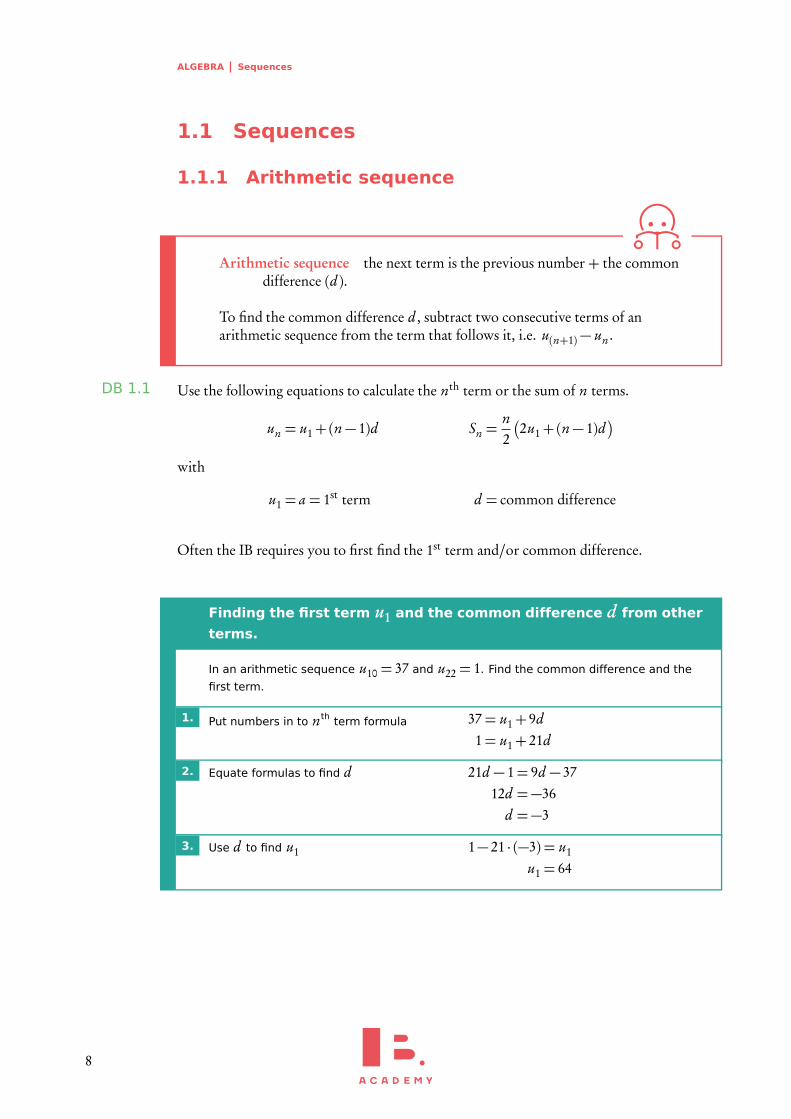
Arithmetic sequence the next term is the previous number + the commondifference (d ).
To find the common difference d , subtract two consecutive terms of anarithmetic sequence from the term that follows it, i.e. u(n+1)− un .
Use the following equations to calculate the nth term or the sum of n terms.DB 1.1
un = u1+(n− 1)d Sn =n2
�
2u1+(n− 1)d�
with
u1 = a = 1st term d = common difference
Often the IB requires you to first find the 1st term and/or common difference.
Finding the first term u1 and the common difference d from other
terms.
In an arithmetic sequence u10 = 37 and u22 = 1. Find the common difference and the
first term.
1. Put numbers in to nth term formula 37= u1+ 9d1= u1+ 21d
2. Equate formulas to find d 21d − 1= 9d − 3712d =−36
d =−3
3. Use d to find u1 1− 21 · (−3) = u1
u1 = 64
8
ALGEBRA Sequences 1
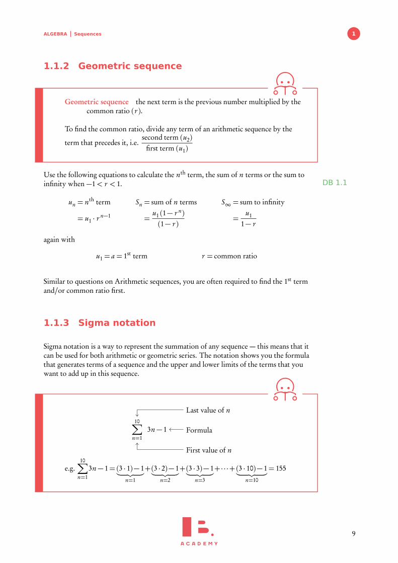
1.1.2 Geometric sequence
Geometric sequence the next term is the previous number multiplied by thecommon ratio (r ).
To find the common ratio, divide any term of an arithmetic sequence by the
term that precedes it, i.e.second term (u2)
first term (u1)
Use the following equations to calculate the nth term, the sum of n terms or the sum toinfinity when −1< r < 1. DB 1.1
un = nth term Sn = sum of n terms S∞ = sum to infinity
= u1 · rn−1 =
u1 (1− r n)(1− r )
=u1
1− r
again with
u1 = a = 1st term r = common ratio
Similar to questions on Arithmetic sequences, you are often required to find the 1st termand/or common ratio first.
1.1.3 Sigma notation
Sigma notation is a way to represent the summation of any sequence — this means that itcan be used for both arithmetic or geometric series. The notation shows you the formulathat generates terms of a sequence and the upper and lower limits of the terms that youwant to add up in this sequence.
10∑
n=13n− 1
Last value of n
Formula
First value of n
e.g.10∑
n=13n− 1= (3 · 1)− 1
︸ ︷︷ ︸
n=1
+(3 · 2)− 1︸ ︷︷ ︸
n=2
+(3 · 3)− 1︸ ︷︷ ︸
n=3
+ · · ·+(3 · 10)− 1︸ ︷︷ ︸
n=10
= 155
9
ALGEBRA Sequences
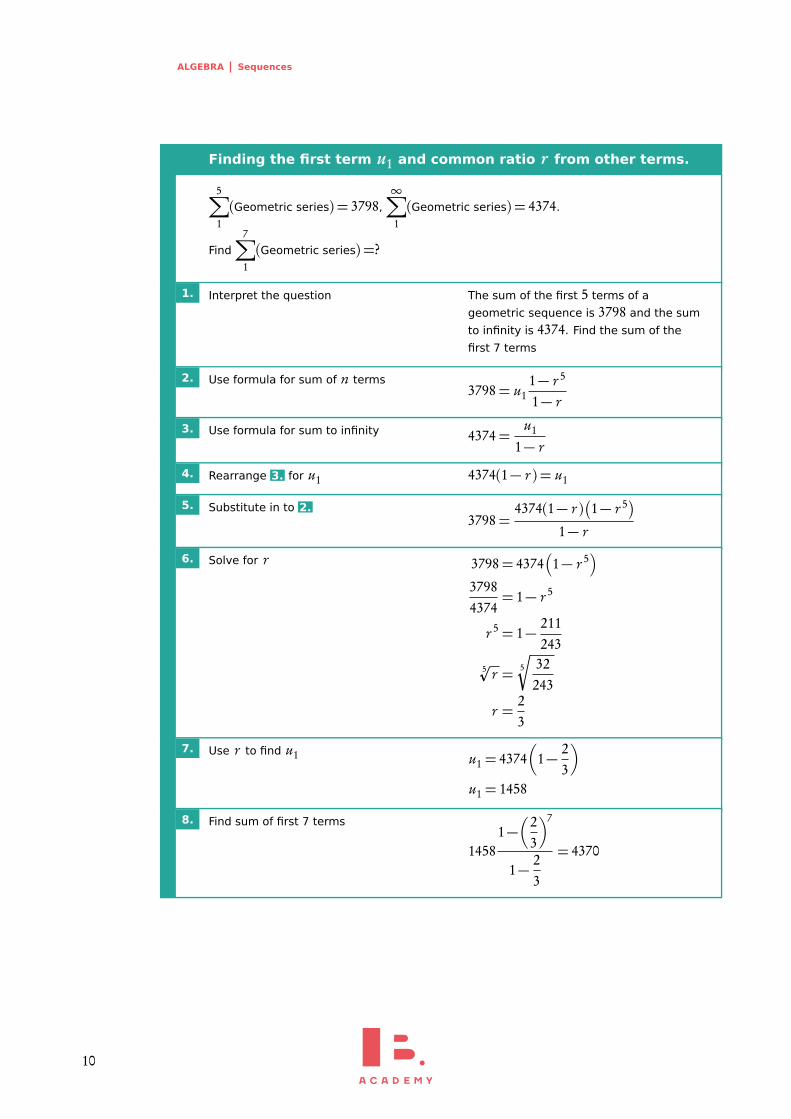
Finding the first term u1 and common ratio r from other terms.
5∑
1(Geometric series) = 3798,
∞∑
1(Geometric series) = 4374.
Find7∑
1(Geometric series) =?
1. Interpret the question The sum of the first 5 terms of a
geometric sequence is 3798 and the sum
to infinity is 4374. Find the sum of the
first 7 terms
2. Use formula for sum of n terms3798= u1
1− r 5
1− r
3. Use formula for sum to infinity 4374=u1
1− r
4. Rearrange 3. for u1 4374(1− r ) = u1
5. Substitute in to 2.3798=
4374(1− r )�
1− r 5�
1− r
6. Solve for r 3798= 4374�
1− r 5�
37984374
= 1− r 5
r 5 = 1− 211243
5pr = 5
s
32243
r =23
7. Use r to find u1 u1 = 4374�
1− 23
�
u1 = 1458
8. Find sum of first 7 terms
14581−
�
23
�7
1− 23
= 4370
10
ALGEBRA Sequences 1
1.1.4 The fundamental theorem of algebra and
complex roots
The fundamental theorem of algebra any polynomial of degree n has nroots
A degree of a polynomial is the largest exponent.
If f (x) = 4x3+ 3x2+ 7x + 9 then it is a polynomial at degree 3, and according to thefundamental theorem of algebra will have 3 roots.
Exam
ple.
Any polynomial can be rewritten/factorized to include the roots:
a(x − r1)(x − r2)(x − r3) · · ·
where r1, r2, r3, . . . , are all roots.
Note: some polynomials will have complex roots. A polynomial of degree 4 can have 4real roots or 4 complex roots or 2 real and 2 complex roots.
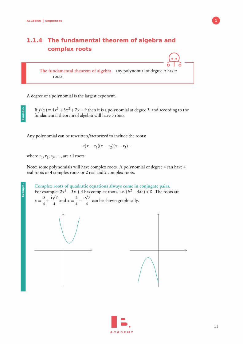
Complex roots of quadratic equations always come in conjugate pairs.For example: 2x2− 3x + 4 has complex roots, i.e. (b 2− 4ac)< 0. The roots are
x =34+
ip
74
and x =34− ip
74
can be shown graphically.
Exam
ple.
11

ALGEBRA Exponents and logarithms
1.2 Exponents and logarithms
1.2.1 Laws of exponents
Exponents always follow certain rules. If you are multiplying or dividing, use thefollowing rules to determine what happens with the powers.
x1 = x 61 = 6
x0 = 1 70 = 1
x m · xn = x m+n 45 · 46 = 411
x m
xn= x m−n 35
34= 35−4 = 31 = 3
(x m)n = x m·n�
105�2= 1010
(x · y)n = xn · yn (2 · 4)3 = 23 · 43 and (3x)4 = 34x4
x−1 =1x
5−1 =15
and�
34
�−1=
43
x−n =1
xn3−5 =
135=
1243
Exam
ple.
1.2.2 Fractional exponents
When doing mathematical operations (+, −, × or ÷) with fractions in the exponent youwill need the following rules. These are often helpful when writing your answers insimplest terms.
x12 =p
x 212 =p
2p
x ·p
x = xp
3 ·p
3= 3p
xy =p
x ·pyp
12=p
4 · 3=p
4 ·p
3= 2 ·p
3
x1n = npx 5
13 = 3p5
xmn = npx m 3−
25 =
15p
32
Exam
ple.
12

ALGEBRA Exponents and logarithms 1
1.2.3 Laws of logarithms
Logarithms are the inverse mathematical operation of exponents, like division is theinverse mathematical operation of multiplication. The logarithm is often used to find thevariable in an exponent. DB 1.2
ax = b ⇔ x = loga b
Since loga ax = x, so that x = loga b .
This formula shows that the variable x in the power of the exponent becomes the subjectof your log equation, while the number a becomes the base of your logarithm.
Below are the rules that you will need to use when performing calculations withlogarithms and when simplifying them. The sets of equations on the left and right arethe same; on the right we show the notation that the DB uses while the equations on theleft are easier to understand.
Laws of logarithms and change of base
DB 1.2I: logA+ logB = log(A ·B) logc a+ logc b = logc (ab )
II: logA− logB = log�
AB
�
logc a− logc b = logc
� ab
�
III: n logA= log(An) n logc a = logc (an)
IV: logB A=logAlogB
logb a =logc alogc b
Note
• x = loga a = 1• With the 4th rule you can change the base of a log.• loga 0= x is always undefined (because ax 6= 0).• When you see a log with no base, it is referring to a logarithm with a base of 10
(e.g. log13= log10 13).
Solve x in exponents using logs.
Solve 2x = 13.
1. Take the log on both sides log2x = log13
2. Use rule III to take x outside x log2= log13
3. Solvex =
log13log2
13

ALGEBRA Binomial expansion
But what about ln and e? These work exactly the same; e is just the irrational number2.71828 . . . (infinitely too long to write out) and ln is just loge.
lna+ ln b = ln(a · b )
lna− ln b = ln� a
b
�
n lna = lnan
lne= 1
elna = a
1.3 Binomial expansion
Binomial an expression (a+ b )n which is the sum of two terms raised to thepower n.
Binomial expansion (a+ b )n is expanded into a sum of terms
Binomial expansions get increasingly complex as the power increases:
binomial binomial expansion(a+ b )1 = a+ b(a+ b )2 = a2+ 2ab + b 2
(a+ b )3 = a3+ 3a2b + 3ab 2+ b 3
The general formula for each term is:�
nr
�
an−r b r .
In order to find the full binomial expansion of a binomial, you have to determine the
coefficient�
nr
�
and the powers for each term, n− r and r for a and b respectively, as
shown by the binomial expansion formula.
Binomial expansion formula
DB 1.3 (a+ b )n = an +�
n1
�
an−1b + · · ·+�
nr
�
an−r b r + · · ·+ b n
=�
n0
�
an +�
n1
�
an−1b +�
n2
�
an−2b 2+ . . .
The powers decrease by 1 for a and increase by 1 for b for each subsequent term.
The sum of the powers of each term will always = n.
14
ALGEBRA Binomial expansion 1
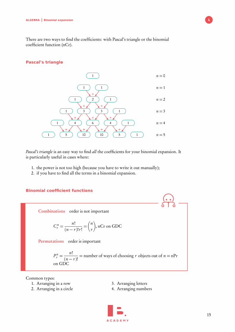
There are two ways to find the coefficients: with Pascal’s triangle or the binomialcoefficient function (nCr).
Pascal’s triangle
1
1 1
1 2+
1
1 3+
3+
1
1 4+
6+
4+
1
1 5+
10+
10+
5+
1
n = 0
n = 1
n = 2
n = 3
n = 4
n = 5
Pascal’s triangle is an easy way to find all the coefficients for your binomial expansion. Itis particularly useful in cases where:
1. the power is not too high (because you have to write it out manually);2. if you have to find all the terms in a binomial expansion.
Binomial coefficient functions
Combinations order is not important
C nr =
n!(n− r )!r !
=�
nr
�
, nCr on GDC
Permutations order is important
P nr =
n!(n− r )!
= number of ways of choosing r objects out of n = nPr
on GDC
Common types:1. Arranging in a row2. Arranging in a circle
3. Arranging letters4. Arranging numbers
15
ALGEBRA Binomial expansion
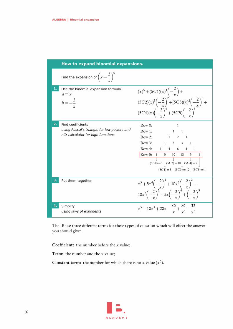
How to expand binomial expansions.
Find the expansion of
�
x − 2x
�5
1. Use the binomial expansion formula
a = x
b =− 2x
(x)5+(5C 1)(x)4�
− 2x
�
+
(5C 2)(x)3�
− 2x
�2+(5C 3)(x)2
�
− 2x
�3+
(5C 4)(x)�
− 2x
�4+(5C 5)
�
− 2x
�5
2. Find coefficients
using Pascal’s triangle for low powers and
nCr calculator for high functions
1
1 1
1 2 1
1 3 3 1
1 4 6 4 1
1 5 10 10 5 1
Row 0:Row 1:Row 2:Row 3:Row 4:Row 5:
(5C 0) = 1
(5C 1) = 5
(5C 2) = 10
(5C 3) = 10
(5C 4) = 5
(5C 5) = 1
3. Put them togetherx5+ 5x4
�
− 2x
�1+ 10x3
�
− 2x
�2+
10x2�
− 2x
�3+ 5x
�
− 2x
�4+�
− 2x
�5
4. Simplify
using laws of exponentsx5− 10x3+ 20x − 80
x+
80x3− 32
x5
The IB use three different terms for these types of question which will effect the answeryou should give:
Coefficient: the number before the x value;
Term: the number and the x value;
Constant term: the number for which there is no x value (x0).
16

ALGEBRA Binomial expansion 1
Finding a specific term in a binomial expansion.
Find the coefficient of x5 in the expansion (2x − 5)8
1. One term is asked, usually of a high
power then use binomial expansion
formula
(a+ b )n = · · ·+�
nr
�
an−r b r + . . .
2. Determine r Since a = 2x , to find x5 we need a5.
a5 = an−r = a8−r , so that r = 3
3. Plug r into the general formula�
nr
�
an−r b r =�
83
�
a8−3b 3 =�
83
�
a5b 3
4. Replace a and b�
83
�
(2x)5(−5)3
5.Use nCr to calculate the value for
�
nr
� �
83
�
= 8C 3= 56
IB ACADEMY
Press menu
5: Probability
3: Combinations
IB ACADEMY
Insert the values for nand r separated by acomma
6. Substitute and calculate the value 56× 25(x5)× (−5)3 =−224000(x5)
7. Alternatively can be found using:�
8!5!3!
�
=�
8× 7× 66
= 8× 7�
17
ALGEBRA Induction
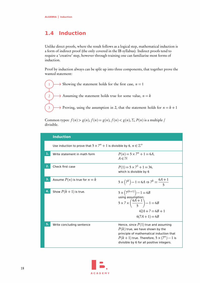
1.4 Induction
Unlike direct proofs, where the result follows as a logical step, mathematical induction isa form of indirect proof (the only covered in the IB syllabus). Indirect proofs tend torequire a ‘creative’ step, however through training one can familiarise most forms ofinduction.
Prrof by induction always can be split up into three components, that together prove thewanted statement:
1
2
3
Showing the statement holds for the first case, n = 1
Assuming the statement holds true for some value, n = k
Proving, using the assumption in 2, that the statement holds for n = k + 1
Common types: f (n)> g (n), f (n) = g (n), f (n)< g (n), Σ, P (n) is a multiple /divisible.
Induction
Use induction to prove that 5× 7n + 1 is divisible by 6, n ∈Z+
1. Write statement in math form P (n) = 5× 7n + 1= 6A,
A∈N
2. Check first case P (1) = 5× 71+ 1= 36,
which is divisible by 6
3. Assume P (n) is true for n = k5×
�
7k�
− 1= 6A⇒ 7k =6A+ 1
5
4. Show P (k + 1) is true. 5�
7(k+1)�
− 1= 6Busing assumption:
5× 7×�
6A+ 15
�
− 1= 6B
42A+ 7= 6B + 16(7A+ 1) = 6B
5. Write concluding sentence Hence, since P (1) true and assuming
P (k) true, we have shown by the
principle of mathematical induction that
P (k + 1) true. Therefore, 5× (7n)− 1 is
divisible by 6 for all positive integers.
18
ALGEBRA Complex numbers 1
1.5 Complex numbers
A complex number is defined as z = a+ b i. Where a, b ∈R, a is the realpart (ℜ) and b is the imaginary part (ℑ).
i=p−1
i2 =−1
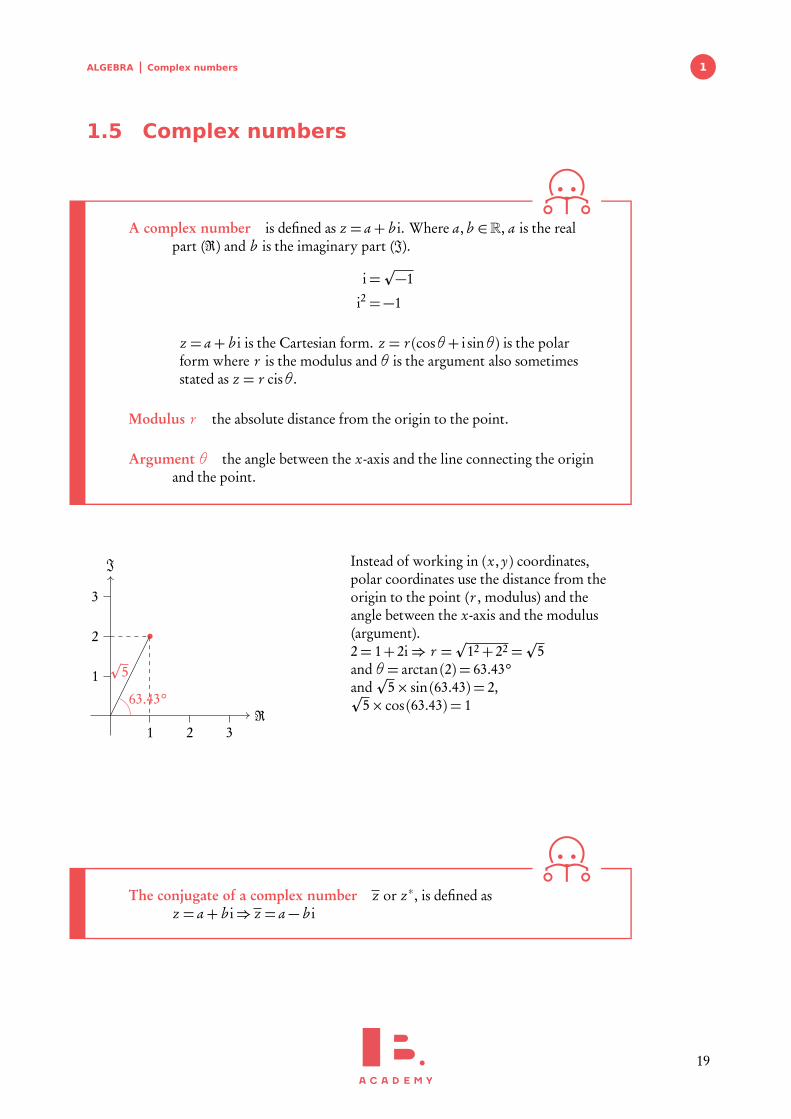
z = a+ b i is the Cartesian form. z = r (cosθ+ i sinθ) is the polarform where r is the modulus and θ is the argument also sometimesstated as z = r cisθ.
Modulus r the absolute distance from the origin to the point.
Argument θ the angle between the x-axis and the line connecting the originand the point.
ℜ
ℑ
1 2 3
1
2
3
p5
63.43°
Instead of working in (x, y) coordinates,polar coordinates use the distance from theorigin to the point (r , modulus) and theangle between the x-axis and the modulus(argument).2= 1+ 2i⇒ r =
p12+ 22 =
p5
and θ= arctan (2) = 63.43°andp
5× sin (63.43) = 2,p5× cos (63.43) = 1
The conjugate of a complex number z or z∗, is defined asz = a+ b i⇒ z = a− b i
19
ALGEBRA Complex numbers
De Moivre’s theorem
DB
zn = (cos x + i sin x)n = cos(nx)+ i sin(nx)
Euler’s formula
eix = cos x + i sin x and (eix )n = einx
De Moivre’s theorem: proof by induction
Having seen the method of induction, we will now apply it to De Moivre’s theorem.
Prove: zn =�
cos(x)i sin(x)�n = cos(nx) + i sin(nx).
1. Show true for n = 1�
cos(x)i sin(x)�1 = cos(1x)+ i sin(1x)
cos(x)i sin(x) = cos(x)+ i sin(1x)
is true for n = 1
2. Assume true for n = k�
cos(x)+ i sin(x)�k = cos(k x)+ i sin(k x)
3. Prove true for n = k + 1�
cos(x)+ i sin(x)�k+1 = cos
�
(k + 1)x�
+ i sin�
(k + 1)x�
=�
cos(x)+ i sin(x)�1�cos(x)+ i sin(x)
�k
Inductive step: use assumption about n = k
=�
cos(x)+ i sin(x)� �
cos(k x)+ i sin(k x)�
Remember i2 =−1
=�
cos(x)� �
cos(k x)�
+�
cos(x)� �
i sin(k x)�
+�
i sin(x)� �
cos(k x)�
−�
sin(x)� �
sin(k x)�
= cos(x)cos(k x)− sin(x) sin(k x)+ i�
cos(x) sin(k x)+ sin(x)cos(k x)�
Use of the double/half angle formulae
= cos�
θ+ kθ�
+ i sin�
θ+ kθ�
= cos�
(k + 1)θ�
+ i sin�
(k + 1)θ�
is required result and form.
Hence, by assuming n = k true, n = k+ 1 is true. Since the statement is true for n = 1, itis true for all n ∈Z+.
20

2FUNCTIONSTable of contents & cheatsheet
Definitions
Function a mathematical relationship where each input has a single output. It is oft en written as f (x)where x is the input
Domain all possible x values, the input. (the domain of investigation)
Range possible y values, the output. (the range of outcomes)
Coordinates uniquely determines the position of a point, given by (x, y)
2.1. Types of functions 22
Linear functions y = mx + c m is the gradient,c is the y intercept.
Midpoint:� x1+ x2
2,
y1+ y2
2
�
Distance:p
(x2− x1)2+(y2− y1)2
Gradient: m =y2− y1
x2− x1
(x1, y1)(x2, y2)
Parallel lines: m1 = m2 (same gradients)Perpendicular lines: m1m2 =−1
Quadratic functions y = ax2+ b x + c = 0
Axis of symmetry: x-coordinate of the vertex: x =−b2a
Factorized form: y = (x + p)(x + q)
x
ya > 0
x
ya < 0
vertex
axis of symetry
If a = 1 use the factorization method (x + p) · (x + q)
If a 6= 1 use the quadratic formula
When asked excplicity complete the square
Vertex form: y = a(x − h)2+ kVertex: (h, k)
Exponentialf (x) = ax + c
f (x)
c
Logarithmicg (x) = loga(x + b )
g (x)
−b
2.2. Rearranging functions 28
Inverse function, f −1(x) reflection of f (x) in y = x.
y = x
f (x)
f −1(x)
Composite function, ( f ◦ g )(x) is the combinedfunction f of g of x.
When f (x) and g (x) are given, replace x in f (x) by g (x).
Transforming functions
Change to f (x) Effect
f (x)+ a Move graph a units upwardsf (x + a) Move graph a units to the lefta · f (x) Vertical stretch by factor a
f (a · x) Horizontal stretch by factor1a
− f (x) Reflection in x-axisf (−x) Reflection in y-axis
21

FUNCTIONS Types of functions
2.1 Types of functions
Functions are mathematical relationships where each input has a single output. You haveprobably been doing functions since you began learning maths, but they may havelooked like this:
16 +10 26 Algebraically this is:f (x) = x + 10,here x = 16, y = 26.
We can use graphs to show multiple outputs of y for inputs x, and therefore visualize therelation between the two. Two common types of functions are linear functions andquadratic functions.
2.1.1 Linear functions
Linear functions y = mx + c increases/decreases at a constant rate m,where m is the gradient and c is the y intercept.
Midpoint� x1+ x2
2,
y1+ y2
2
�
DistanceÆ
(x2− x1)2+(y2− y1)2
Gradient m =y2− y1
x2− x1
Parallel lines m1 = m2 (equal gradients)Perpendicular lines m1m2 =−1
-1
-1
1
1
2
2
3
3
Determine the midpoint, distance and gradient using the two points P1(2, 8)and P2(6, 3)
Midpoint:� x1+ x2
2,
y1+ y2
2
�
=�
2+ 62
,8+ 3
2
�
= (4,5.5)
Distance:p
(x2− x1)2+(y2− y1)2 =p
(6− 2)2+(3− 8)2 =p
(4)2+(5)2 =p
41
Gradient: m =y2− y1
x2− x1= m =
3− 86− 2
=−54
Parallel line: −54
x + 3
Perpendicular line: −45
x + 7x
y
1 2 3 4 5 6 7
123456789 P1(2,8)
P2(6,3)
Exam
ple.
22

FUNCTIONS Types of functions 2
2.1.2 Quadratic functions
x
y
O
a > 0
a > 0, positive quadratic
x
y
O
a < 0
a < 0, negative quadratic
Quadratic functions y = ax2+ b x + c = 0
Graph has a parabolic shape, increase/decrease at an increasing rate.
The roots of an equation are the x-values for which y = 0, in other words thex-intercept(s).
To find the roots of the equation you can use
factorisation: If a = 1, use the factorization method (x + p) · (x + q)
quadratic formula: If a 6= 1, use the quadratic formulaThe b 2 − 4ac part ofthe quadratic formulais also known as thediscriminant ∆. It canbe used to check howmany x-intercepts theequation has:∆> 0: 2 solutions∆= 0: 1 solution∆< 0: no real solutions
−b ±p
b 2− 4ac2a
=−b ±
p∆
2a
Solving quadratic equations by factorisation.
Solve: x2− 5x + 6= 0
1. Set up system of equations
p + q = b and p × q = cp + q =−5p × q = 6
«
p =−2 and q =−3
2. Plug the values for p and q into:
(x + p)(x + q)(x − 2)(x − 3) = x2− 5x + 6
3. Equate each part to 0(x + p) = 0, (x + q) = 0,
and solve for x
(x − 2) = 0(x − 3) = 0
«
x = 2 or x = 3
23

FUNCTIONS Types of functions
Solving quadratic equations using the quadratic formula.
Solve: 3x2− 8x + 4= 0
1. Calculate the discriminant∆∆= b 2− 4ac
∆= (−8)2− 4 · 3 · 4= 16
2. How many solutions?
∆> 0⇒ 2 solutions
∆= 0⇒ 1 solution
∆< 0⇒ no real solutions
∆> 0, so 2 solutions
3. Calculate x , use
x =−b ±
p∆
2a
x =8±p
162 · 3
=8± 4
6
=8− 4
6=
46
=8+ 4
6= 2
⇒ x =23
or x = 2
By completing the square you can find the value of the vertex (the minimum ormaximum). For the exam you will always be asked explicitly.
Find the vertex by completing the square
4x2− 2x − 5= 0
1. Move c to the other side 4x2− 2x = 5
2. Divide by a x2− 12
x =54
3.Calculate
� x coeficient
2
�2
−12
2
2
=116
4. Add this term to both sides x2− 12
x +116=
54+
116
5. Factor perfect square, bring constant
back
�
x − 14
�2− 21
16= 0
⇒ minimum point=
�
14
,−2116
�
Other forms: y = a(x − h)2+ k vertex (h, k) and y = a(x − p)(x − q), x intercepts:(p, 0)(q , 0).
24

FUNCTIONS Types of functions 2
2.1.3 Functions with asymptotes
Asymptote a straight line that a curve approaches, but never touches.
A single function can have multiple asymptotes: horizontal, vertical and in rare casesdiagonal. Functions that contain the variable (x) in the denominator of a fraction willalways have asymptotes, as well as exponential and logarithmic functions.
Vertical asymptotes
Vertical asymptotes occur when the denominator is zero, as dividing by zero isundefinable. Therefore if the denominator contains x and there is a value for x for whichthe denominator will be 0, we get a vertical asymptote.
In the function f (x) =x
x − 4, when x = 4, the denominator is 0 so there is a vertical
asymptote.Exam
ple.
Horizontal asymptotes
Horizontal asymptotes are the value that a function tends to as x become really big orreally small; technically: to the limit of infinity, x→∞. When x is large other parts ofthe function not involving x become insignificant and so can be ignored.
In the function f (x) =x
x − 4, when x is small the 4 is important.
x = 10 10− 4= 6But as x gets bigger the 4 becomes increasingly insignificant
x = 100 100− 4= 96x = 10000 10000− 4= 9996
Therefore as we approach the limits we can ignore the 4.lim
x→∞f (x) =
xx= 1
So there is a horizontal asymptote at y = 1.
Exam
ple.
Exponential and logarithmic functions
Exponential functions willalways have a horizontalasymptote and logarithmicfunctions will always have avertical asymptote, due to thenature of these functions. Theposition of the asymptote isdetermined by constants in thefunction.
Exponential
f (x)
c
f (x) = ax + cwhere a is a positive number
(often e)
Logarithmic
g (x)
−b
g (x) = loga(x + b )
25

FUNCTIONS Types of functions
2.1.4 Describing functions
Even and odd functions
When f (x) = f (−x) we describe the function as even or a graph symmetrical over they-axis.
An even function: f (x) = x4 + 2
Testing algebraically substitute (−x): f (−x) =−x4+ 2= x4+ 2
x
y
The graph is symmetrical over the y-axis.
Exam
ple.
When − f (x) = f (−x) we describe the function as odd or a graph has rotationalsymmetry with respect to the origin.
An odd function: f (x) = x3 − x
Testing algebraically. − f (x) =−x3+ x.Substitute (−x): f (−x) =−x3+ x =−x3+ x =− f (x)
x
y
The graph has a rotational symmetry with respect to the origin.
Exam
ple.
26
FUNCTIONS Types of functions 2
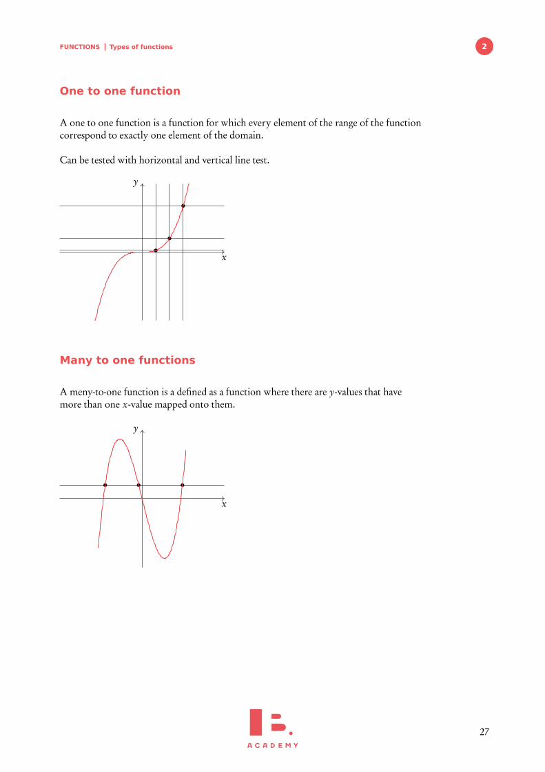
One to one function
A one to one function is a function for which every element of the range of the functioncorrespond to exactly one element of the domain.
Can be tested with horizontal and vertical line test.
x
y
Many to one functions
A meny-to-one function is a defined as a function where there are y-values that havemore than one x-value mapped onto them.
x
y
27

FUNCTIONS Rearranging functions
2.2 Rearranging functions
2.2.1 Inverse functions, f −1(x)
Inverse functions are the reverse of a func-tion. Finding the input x for the output y.You can think of it as going backwardsthrough the number machine
f −1(x)
This is the same as reflecting a graph in the y = x axis.
Finding the inverse function.
f (x) = 2x3+ 3, find f −1(x)
1. Replace f (x) with y y = 2x3+ 3
2. Solve for x y − 3= 2x3
⇒y − 3
2= x3
⇒ 3
s
y − 32= x
3. Replace x with f −1(x) and y with x 3
s
x − 32= f −1(x)
2.2.2 Composite functions
Composite functions are combination of two functions.
( f ◦ g )(x) means f of g of x
To find the composite function above substitute the function of g (x) into the x of f (x).
Let f (x) = 2x + 3 and g(x) = x2. Find (f ◦ g)(x) and (g ◦ f )(x).
( f ◦ g )(x): replace x in the f (x) function with the entire g (x) function
(2g (x))+ 3= 2x2+ 3
(g ◦ f )(x): replace x in the g (x) function with the entire f (x) function
�
f (x)�2 = (2x + 3)2
Exam
ple.
28

FUNCTIONS Rearranging functions 2
2.2.3 Transforming functions
By adding and/ormultiplying by constantswe can transform afunction into anotherfunction.
Exam hint: describethe transformation withwords as well to guaran-tee marks.
Change to f (x) Effect
f (x)+ a Move graph a units upwardsf (x + a) Move graph a units to the lefta · f (x) Vertical stretch by factor af (a · x) Horizontal stretch by factor 1/a− f (x) Reflection in x-axisf (−x) Reflection in y-axis
Transforming functions f (x)→ a f (x + b)
Given f (x) =14
x3+ x2− 54
x , draw 3 f (x − 1).
1. Sketch f (x)
x
y
−3−2−1 1 2 3
−3−2−1
123
f (x)
2. Stretch the graph by the factor of a a = 3
x
y
−3−2−1 1 2 3
−3−2−1
123
f (x)3 f (x)
3. Move graph by −b Move graph by 1 to the right
x
y
−3−2−1 1 2 3
−3−2−1
123
f (x) 3 f (x − 1)
29

FUNCTIONS Rearranging functions
Absolute value:�
�f�
�
f (x) = x2− 2⇒�
� f (x)�
�=?.
x
y
−3 −2 −1 1 2 3
−3
−2
−1
1
2
3f (x) = x2− 2
�
� f (x)�
�
Exam
ple.
Reciprocal:1
f (x)
f (x) = x4+ 4x3 so:1
f (x)=
1x4+ 4x3
x
y
−4 −3 −2 −1 1 2 3 4
−40
−30
−20
−10
10
20
30
40
f (x) = x4+ 4x3
1f (x)
Exam
ple.
30
FUNCTIONS Rearranging functions 2
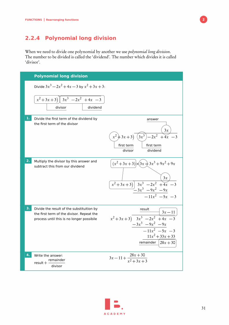
2.2.4 Polynomial long division
When we need to divide one polynomial by another we use polynomial long division.The number to be divided is called the ‘dividend’. The number which divides it is called‘divisor’.
Polynomial long division
Divide 3x3− 2x2+ 4x − 3 by x2+ 3x + 3:
x2+ 3x + 3�
3x3 − 2x2 + 4x − 3
divisor dividend
1. Divide the first term of the dividend by
the first term of the divisor
3x
x2+ 3x + 3�
3x3 − 2x2 + 4x − 3
first term
divisor
first term
dividend
answer
2. Multiply the divisor by this answer and
subtract this from our dividend(x2+ 3x + 3)× 3x = 3x3+ 9x2+ 9x
3x
x2+ 3x + 3�
3x3 − 2x2 + 4x − 3− 3x3 − 9x2 − 9x
− 11x2 − 5x − 3
3. Divide the result of the substituition by
the first term of the divisor. Repeat the
process until this is no longer possibile
3x − 11
x2+ 3x + 3�
3x3 − 2x2 + 4x − 3− 3x3 − 9x2 − 9x
− 11x2 − 5x − 311x2+ 33x + 33
28x + 30
result
remainder
4. Write the answer:
result+remainder
divisor
3x − 11+28x + 30
x2+ 3x + 3
31
FUNCTIONS The factor and remainder theorem
2.3 The factor and remainder theorem
Remainder theorem when we divide a polynomial f (x) by x − c theremainder r equals f (c)
Let’s sayf (x)÷ (x − c) = q(x)+ r
where r is the remainder. We also know
f (x) = (x − c)q(x)+ r
If we now substitute x with c
f (c) = (c − c)q(c)+ r
but c − c = 0, thereforef (c) = r
Factor theorem when f (c) = 0 then x − c is a factor of the polynomial
32

3VECTORSTable of contents & cheatsheet
Definitions
Vector a geometric object with magnitude (length) anddirection, represented by an arrow.
Collinear points points that lie on the same lineUnit vector vector with magnitude 1
Base vector ~i =
100
, ~j =
010
, ~k =
001
.
3.1. Working with vectors 34
Vector from point O to point A: ~OA= ~a =�
32
�
Vector from point O to point B : ~OB = ~b =�
−11
�
Can be written in two ways:
~a =
320
=�
32
�
~a = 3i + 2 j + 0k = 3i + 2 j
Length of ~a: |~a|=p
x2+ y2 =p
32+ 22 =p
13
Addition & multiplication: ~a+ 2~b =�
32
�
+ 2�
−11
�
=�
32
�
+�
−22
�
=�
14
�
Subtraction: ~a− ~b =�
32
�
−�
−11
�
=�
41
�
x
y
−1 1 2 3 4
1
2
3
4
A
~aB
~b
3.2. Equations of lines 36
Example of a line:
r =�
03
�
+ t�
11
�
position vectorparameter
direction vector
x
y
−3−2−1 1 2 3
12345 y = x + 3
t�
11
�
�
03
�
3.3. Dot product 38
The dot product of two vectors ~c · ~d can beused to find the angle between them.
Let ~c =
c1c2c3
, ~d =
d1d2d3
:
~c · ~d = |~c || ~d |cosθ
~c · ~d = c1d1+ c2d2+ c3d3
33

VECTORS Working with vectors
3.1 Working with vectors
Vectors are a geometric object with a magnitude (length) and direction. They arerepresented by an arrow, where the arrow shows the direction and the length representsthe magnitude.
So looking at the diagram we can see thatvector ~u has a greater magnitude than ~v.Vectors can also be described in terms of thepoints they pass between. So
(
~u = ~PQ~v = ~P S
with the arrow over the top showing thedirection.
~v
~uP Q
RS M
N
You can use vectors as a geometric algebra, expressing other vectors in terms of ~u and ~v.For example
~P R= ~u + ~v ~QS =−~u + ~v ~QN =12(−~u + ~v)
~u
~v
P Q
RS M
N~v
−~uP Q
RS M
N
~u−1
2~u
12~v
P Q
RS M
This may seem slightly counter-intuitive at first. But if we add in some possible figuresyou can see how it works. If ~u moves 5 units to the left and ~v moves 1 unit to the right(−left) and 3 units down.
Then ~P R= ~u + ~v = 5 units to the left −1 unit to the right and 3 units down = 4 units tothe left and 3 units down.
34

VECTORS Working with vectors 3
3.1.1 Vectors with value
Formally the value of a vector is defined by its direction and magnitude within a 2D or3D space. You can think of this as the steps it has to take to go from its starting point toits end, moving only in the x, y and z axis.
Vector from point O to point A:
~OA= ~a =�
32
�
Vector from point O to point B :
~OB = ~b =�
−11
�
x
y
−1 1 2 3 4
1
2
3
4
A
~aB
~b
Note: unless told other-wise, answer questionsin the form used in thequestion.
Vectors can be written in two ways:
1. ~a =
320
=�
32
�
, where the top value is movement in the x-axis. Then the next is
movement in the y and finally in the z. Here the vector is in 2D space as there isno value for the z-axis.
2. as the sum of the three base vectors:
~i =
100
, ~j =
010
, ~k =
001
.
Here ~i is moving 1 unit in the x-axis, ~j 1 unit in the y-axis and ~k 1 unit in the z-axis.
~a = 3i + 2 j + 0k = 3i + 2 j
When we work with vectors we carry out the mathematical operation in each axisseparately. So x-values with x-values and so on.
Addition & multiplication:
~a+2~b =�
32
�
+2�
−11
�
=�
32
�
+�
−22
�
=�
14
�
Subtraction:
~a− ~b =�
32
�
−�
−11
�
=�
41
�
x
y
−1 1 2 3 4
1
2
3
4
A
~aB
~b
~a+ 2~b
~a− ~b
~b
~b
−~b
However it must be remembered that vector notation does not give us the actual length(magnitude) of the vector. To find this we use something familiar.
35
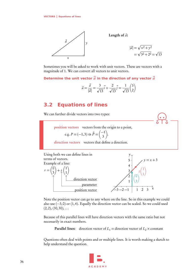
VECTORS Equations of lines
x
y~a
Length of ~a:
|~a|=p
x2+ y2
=p
32+ 22 =p
13
Sometimes you will be asked to work with unit vectors. These are vectors with amagnitude of 1. We can convert all vectors to unit vectors.
Determine the unit vector ba in the direction of any vector ~a
ba =~a|~a|=
3p
13~i +
2p
13~j =
1p
13
�
32
�
3.2 Equations of lines
We can further divide vectors into two types:
position vectors vectors from the origin to a point,
e.g. P = (−1,3)⇒ ~P =�
−13
�
.
direction vectors vectors that define a direction.
Using both we can define lines interms of vectors.Example of a line:
r =�
03
�
+ t�
11
�
position vectorparameter
direction vector
x
y
−3−2−1 1 2 3
12345 y = x + 3
t�
11
�
�
03
�
Note the position vector can go to any where on the line. So in this example we couldalso use (−3,0) or (1,4). Equally the direction vector can be scaled. So we could used(2,2), (30,30), . . .
Because of this parallel lines will have direction vectors with the same ratio but notnecessarily in exact numbers.
Parallel lines: direction vector of L1 = direction vector of L2× constant
Questions often deal with points and or multiple lines. It is worth making a sketch tohelp understand the question.
36
VECTORS Equations of lines 3
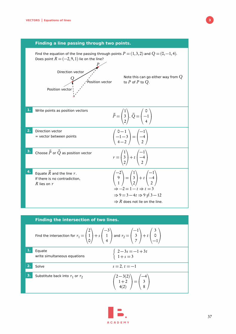
Finding a line passing through two points.
Find the equation of the line passing through points P = (1,3,2) and Q = (0,−1,4).Does point R= (−2,9,1) lie on the line?
Q
P
Position vector
Position vector
Direction vectorNote this can go either way from Qto P of P to Q .
1. Write points as position vectors~P =
132
, ~Q =
0−14
2. Direction vector
= vector between points
0− 1−1− 34− 2
=
−1−42
3. Choose ~P or ~Q as position vectorr =
132
+ t
−1−42
4. Equate ~R and the line r .
If there is no contradiction,
R lies on r
−291
=
132
+ t
−1−42
⇒−2= 1− t ⇒ t = 3⇒ 9= 3− 4t ⇒ 9 6= 3− 12⇒ R does not lie on the line.
Finding the intersection of two lines.
Find the intersection for r1 =
210
+ s
−314
and r2 =
−137
+ t
30−1
1. Equate
write simultaneous equations
�
2− 3s =−1+ 3t1+ s = 3
2. Solve s = 2, t =−1
3. Substitute back into r1 or r2
2− 3(2)1+ 24(2)
=
−438
37
VECTORS Dot (scalar) product
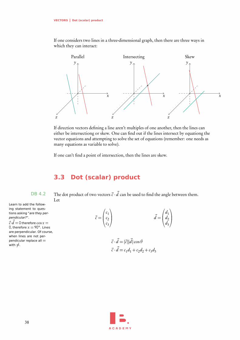
If one considers two lines in a three-dimensional graph, then there are three ways inwhich they can interact:
Parallely
x
z
Intersectingy
x
z
Skewy
x
z
If direction vectors defining a line aren’t multiples of one another, then the lines caneither be intersectiong or skew. One can find out if the lines intersect by equationg thevector equations and attempting to solve the set of equations (remember: one needs asmany equations as variable to solve).
If one can’t find a point of intersection, then the lines are skew.
3.3 Dot (scalar) product
The dot product of two vectors ~c · ~d can be used to find the angle between them.DB 4.2Let
Learn to add the follow-ing statement to ques-tions asking “are they per-pendicular?”.
~c · ~d = 0 therefore cos x =0, therefore x = 90°. Linesare perpendicular. Of course,when lines are not per-pendicular replace all =with 6=.
~c =
c1c2c3
~d =
d1d2d3
~c · ~d = |~c || ~d |cosθ
~c · ~d = c1d1+ c2d2+ c3d3
38
VECTORS Cross (vector) product 3
Finding the angle between two lines.
(Often are these two vectors perpendicular)
Find the angle between
23−1
and
813
.
1.Find ~c · ~d in terms of components ~c · ~d = 2× 8+ 3× 1+(−1)× 3= 16
2.Find ~c · ~d in terms of magnitudes ~c · ~d =
p
22+ 32+(−1)2×p
82+ 12+ 32× cosθ=p
14p
74cosθ
3. Equate and solve for θ 16=p
14p
74cosθ
⇒ cosθ=16
p14p
74⇒ θ= 60.2°
Note: when θ= 90° (perpendicular vectors), cos(90°) = 0⇒ ~c · ~d = 0
3.4 Cross (vector) product
The cross product of two vectors produces a third vector which is perpendicular to bothof the two vectors. As the result is a vector, it is also called the vector product.
There are two methods to find the cross product:
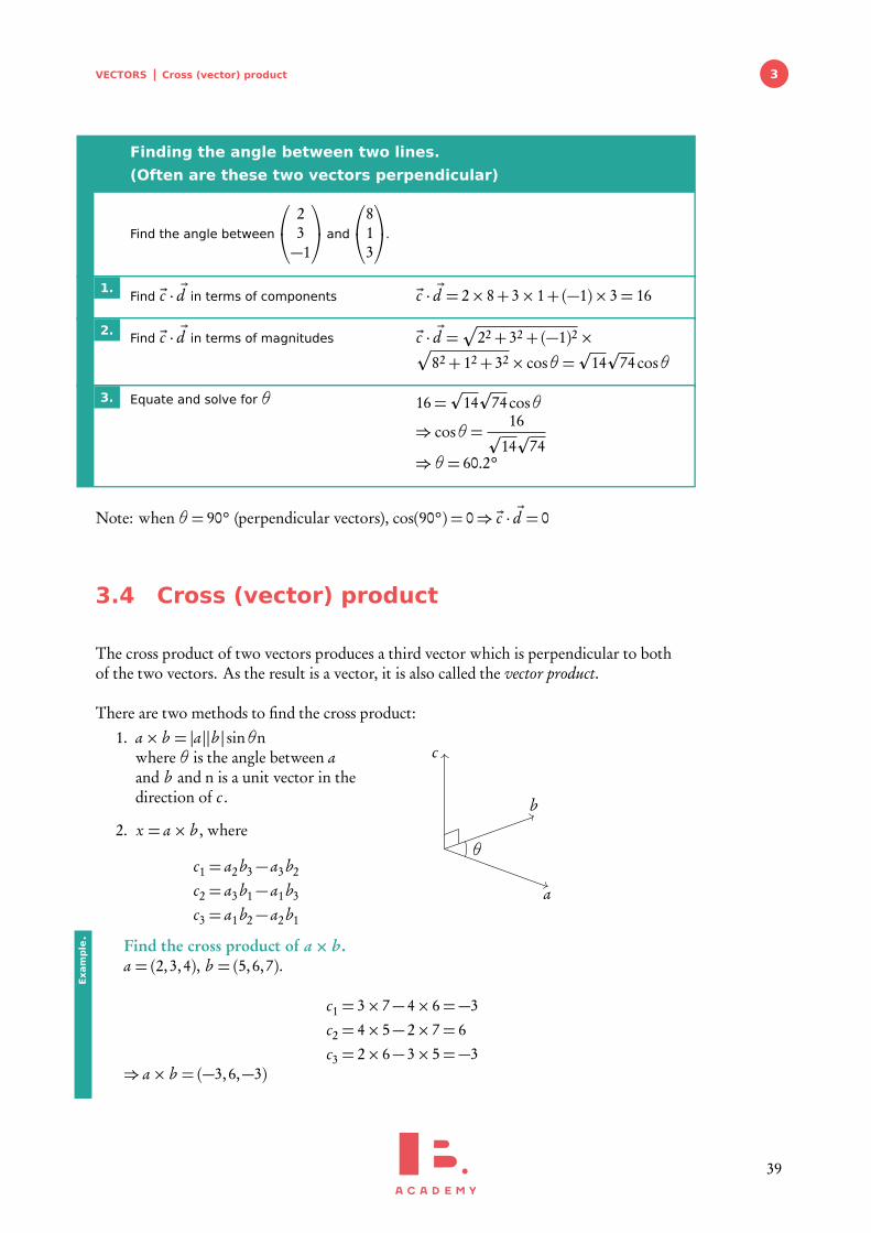
1. a× b = |a||b | sinθnwhere θ is the angle between aand b and n is a unit vector in thedirection of c .
2. x = a× b , where
c1 = a2b3− a3b2
c2 = a3b1− a1b3
c3 = a1b2− a2b1
a
b
c
θ
Find the cross product of a × b.a = (2,3,4), b = (5,6,7).
c1 = 3× 7− 4× 6=−3c2 = 4× 5− 2× 7= 6c3 = 2× 6− 3× 5=−3
⇒ a× b = (−3,6,−3)
Exam
ple.
39
VECTORS Equation of a plane
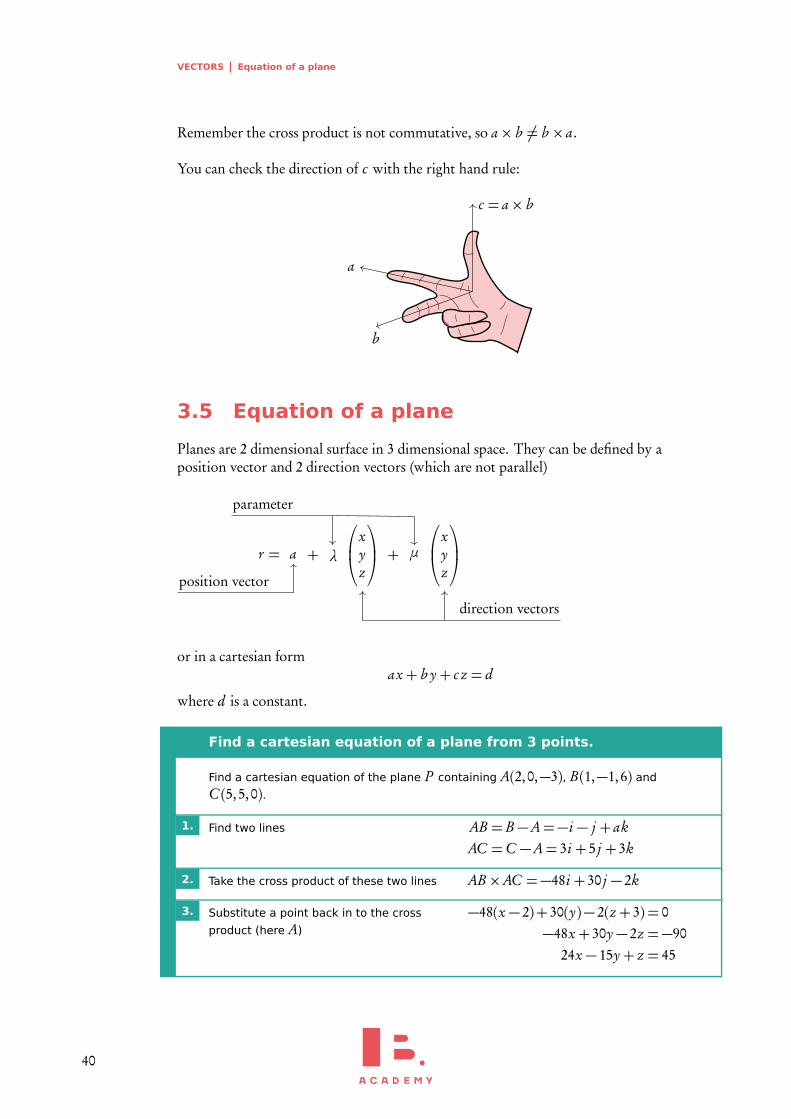
Remember the cross product is not commutative, so a× b 6= b × a.
You can check the direction of c with the right hand rule:
c = a× b
a
b
3.5 Equation of a plane
Planes are 2 dimensional surface in 3 dimensional space. They can be defined by aposition vector and 2 direction vectors (which are not parallel)
r = a + λ
xyz
+ µ
xyz
position vector
parameter
direction vectors
or in a cartesian formax + b y + c z = d
where d is a constant.
Find a cartesian equation of a plane from 3 points.
Find a cartesian equation of the plane P containing A(2,0,−3), B(1,−1,6) and
C (5,5,0).
1. Find two lines AB = B −A=−i − j + akAC =C −A= 3i + 5 j + 3k
2. Take the cross product of these two lines AB ×AC =−48i + 30 j − 2k
3. Substitute a point back in to the cross
product (here A)
−48(x − 2)+ 30(y)− 2(z + 3) = 0−48x + 30y − 2z =−90
24x − 15y + z = 45
40
VECTORS Equation of a plane 3
3.5.1 Line and plane
Lines can instersect with a plane in 3 ways:
1. Parallel to the plane 0 solutions
2. Intersect the plane 1 solution
3. Lie on the plane infinite solutions
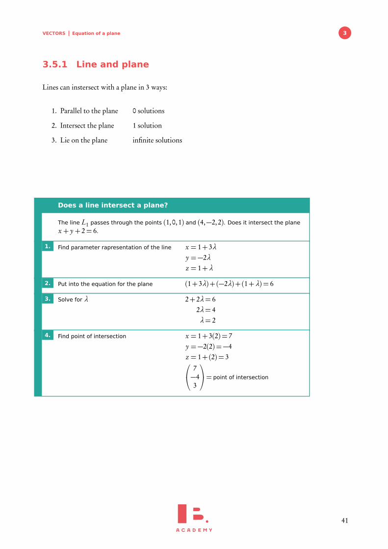
Does a line intersect a plane?
The line L1 passes through the points (1,0,1) and (4,−2,2). Does it intersect the plane
x + y + 2= 6.
1. Find parameter rapresentation of the line x = 1+ 3λy =−2λz = 1+λ
2. Put into the equation for the plane (1+ 3λ)+ (−2λ)+ (1+λ) = 6
3. Solve for λ 2+ 2λ= 62λ= 4λ= 2
4. Find point of intersection x = 1+ 3(2) = 7y =−2(2) =−4z = 1+(2) = 3
7−43
= point of intersection
41

VECTORS Equation of a plane
3.5.2 Plane and plane
Intersection of two planes
When two planes intersect, they will intersect along a line.
Finding line of intersection of two planes
Find the intersection of x + y + z + 1= 0 and x + 2y + 3z + 4= 0
1. Check the equations for planes are in a
cartesian form; move the constant to the
other side
�
x + y + z =−1 (1)
x + 2y + 3z =−4 (2)
2. Solve the system of equations to remove
a variable
(1)− (2)�
x + y + z =−1−x − 2y − 3z =−4− y − 2z = 3
y =−3− 2z
3. Let z = t ⇒ y =−3− 2t . Rearrange:
x =−1− y − zx =−1− (−3− 2t )− tx = t + 2
4. Find the result Intersection occurs at line
(x, y, z) = (t + 2,−2t − 3, t ) or
r =
2−30
+
1−21
t
42

VECTORS Equation of a plane 3
Intersection of three planes
Unless two or more planes are parallel, three planes will intersect at a point. If two areparallel there will be two lines of intersect. If all three are parallel, there will be nosolutions.
We have three variablesand three equations andse we can solve the sys-tem.
Finding point of intersect of three planes
Find the instersect of the three planes
x − 3y + 3z =−4 (a)
2x + 3y − z = 15 (b)
4x − 3y − z = 19 (c)
1. Eliminate one variable in two pair of lines
(here z)
(b)− (c)⇒ −2x + 6y =−4 (d)
(a)+ 3(b)⇒ 7x + 6y = 41 (e)
2. Eliminate antoher variable from these
new lines (here y)
(e)− (d)⇒ 9x = 45x = 5
3. Place the value into the equations to find
values for x , y , and zx = 5
(d) − 2(5)+ 6y =−4 ⇒ y = 1(a) (5)− 3(1)+ 3z =−4 ⇒ z =−2Point of intersection (5,1,−2)
3.5.3 Normal vector
By taking the cross product of the two direction vectors that define a plane, we can findthe normal vector. This vector is perpendicular to the plane. In turn the normal vectorcan be used to show a line is parallel to the plane by using the dot product. If paralleln · d = 0, where n is the normal vector and d is the direction vector of a line.
43


4TRIGONOMETRY AND
CIRCULAR FUNCTIONSTable of contents & cheatsheet
4.1. Basic trigonometry 46
radians=π
180°× degrees degrees=
180°π× radians
Before each question make sure calculator is in correctsetting: degrees or radians?
chord
segment
arc
sector
Area of a sector =12
r 2 ·θ
Arc length = r ·θ
θ in radians, r = radius.
Right-angle triangle (triangle with 90° angle)
adjacent
hypo
tenus
e
θ oppo
site sinθ=
oppositehypotenuse
SOH
cosθ=adjacent
hypotenuseCAH
tanθ=oppositeadjacent
TOA
Non-right angle triangles
a
bc
B C
A
Sine rule:a
sinA=
bsinB
=c
sinCUse this rule when you know: 2 angles and a side (notbetween the angles) or 2 sides and an angle (notbetween the sides).
Cosine rule: c2 = a2+ b 2− 2 ab cosCUse this rule when you know: 3 sides or 2 sides andthe angle between them.
Area of a triangle: Area=12
ab sinC
Use this rule when you know: 3 sides or 2 sides andthe angle between them.
Three-figure bearingsDirection given as an angle of a full circle. North is 000 and the angle is expressed in the clockwise direction from North.So East is 090, South is 180 and West 270.
4.2. Circular functions 51
sin90°= 1
cos0°= 1
positive angles
αβ
θ
deg 0° 30° 45° 60° 90° 120° 135° 150° 180°
rad 016π
14π
13π
12π
23π
34π
56π π
sinθ 012
p2
2
p3
21
p3
2
p2
212
0
cosθ 1
p3
2
p2
212
0 −12
−p
22
−p
32
−1
tanθ 01p
31
p3 ∞ −
p3 −1 − 1
p3
0
Trigonometric function y = a sin(b x + c)+ d
Amplitude: a
Period:360°
bor
2πb
Horizontal shift: c
Vertical shift: d
Trigonometric identities
tanθ=sinθcosθ
sin2 θ+ cos2 θ= 1
2sinθ cosθ= sin2θ
cos2θ= cos2 θ− sin2 θ
45

TRIGONOMETRY AND CIRCULAR FUNCTIONS Basic trigonometry
4.1 Basic trigonometry
This section offers an overview of some basic trigonometry rules and values that willrecur often. It is worthwhile to know these by heart; but it is much better to understandhow to obtain these values. Like converting between Celsius and Fahrenheit; you canremember some values that correspond to each other but if you understand how toobtain them, you will be able to convert any temperature.
4.1.1 Converting between radians and degrees
radians=π
180°× degrees
degrees=180°π× radians
30°
π
645°
π
460°
π
390°
π
2
120°
2π3
135°
3π4
150°
5π6
180°π
270°
3π2
0° 0
360° 2π
Table 4.1: Common radians/degrees conversions
Degrees 0° 30° 45° 60° 90° 120° 135° 180° 270° 360°
Radians 0π
6π
4π
3π
22π3
3π4
π3π2
2π
4.1.2 Circle formulasDB 3.1
Area of a sector =12
r 2 ·θ
Arc length = r ·θ
θ in radians, r = radius.
chord
segment
arc
sector
46

TRIGONOMETRY AND CIRCULAR FUNCTIONS Basic trigonometry 4
4.1.3 Right-angle triangles
a2 = b 2+ c2 Pythagoras
sinθ=opposite
hypotenuseSOH
cosθ=adjacent
hypotenuseCAH
tanθ=oppositeadjacent
TOA adjacent
hypo
tenus
e
θ
opposite
Two important triangles to memorize:
4
53
12
135
The IB loves asking questions about these special triangles which have whole numbersfor all the sides of the right triangles.
60°
30°
1
p3
2
45°
45°
1
1
p2
Note: these triangles can help you in finding the sin, cos and tan of the angles that youshould memorize, shown in table 4.2 at page 52. Use SOH, CAH, TOA to find thevalues.
47
TRIGONOMETRY AND CIRCULAR FUNCTIONS Basic trigonometry
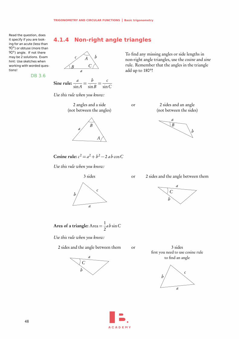
4.1.4 Non-right angle triangles
a
bc
B C
ATo find any missing angles or side lengths innon-right angle triangles, use the cosine and sinerule. Remember that the angles in the triangleadd up to 180°!
Read the question, doesit specify if you are look-ing for an acute (less than90°) or obtuse (more than90°) angle. If not theremay be 2 solutions. Examhint: Use sketches whenworking with worded ques-tions!
DB 3.6
Sine rule:a
sinA=
bsinB
=c
sinC
Use this rule when you know:
2 angles and a side(not between the angles)
a
A
B
or 2 sides and an angle(not between the sides)
b
aB
Cosine rule: c2 = a2+ b 2− 2 ab cosC
Use this rule when you know:
3 sides
a
cb
or 2 sides and the angle between them
b
aC
Area of a triangle: Area=12
ab sinC
Use this rule when you know:
2 sides and the angle between them
b
aC
or 3 sidesfirst you need to use cosine rule
to find an angle
a
cb
48
TRIGONOMETRY AND CIRCULAR FUNCTIONS Basic trigonometry 4
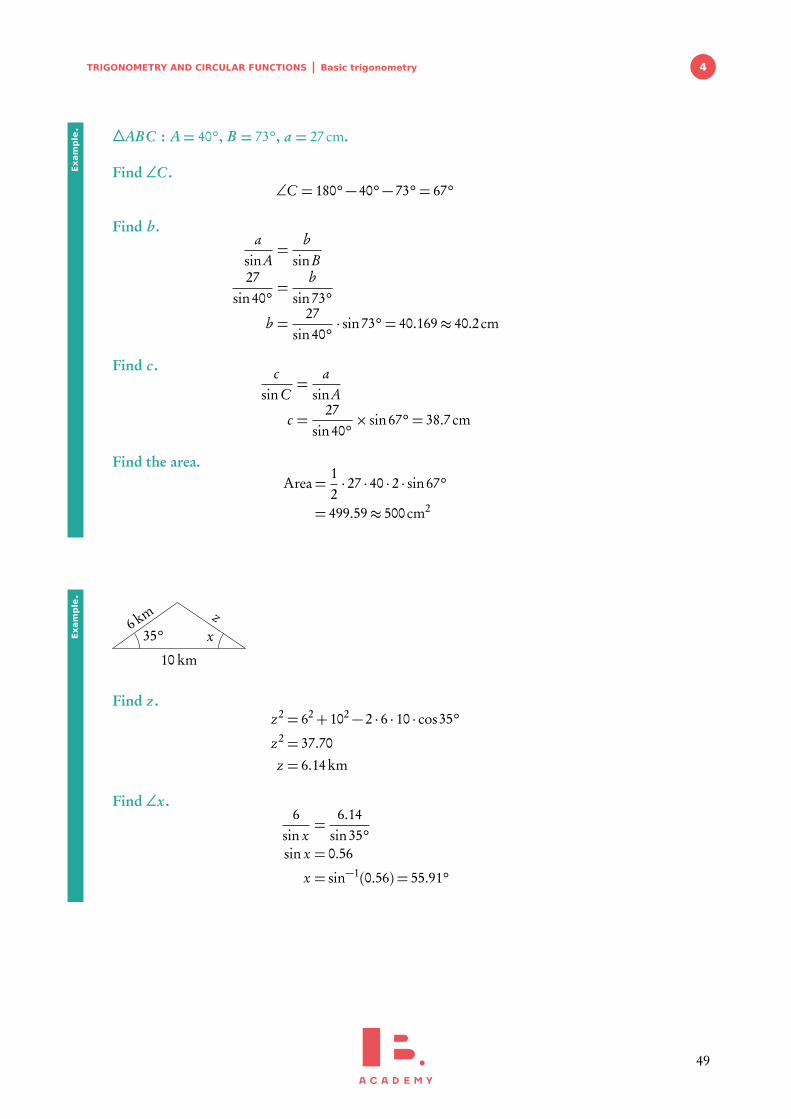
4ABC : A= 40°, B = 73°, a = 27 cm.
Find ∠C.∠C = 180°− 40°− 73°= 67°
Find b.a
sinA=
bsinB
27sin40°
=b
sin73°
b =27
sin40°· sin73°= 40.169≈ 40.2cm
Find c . csinC
=a
sinA
c =27
sin40°× sin67°= 38.7cm
Find the area.Area=
12· 27 · 40 · 2 · sin67°
= 499.59≈ 500cm2
Exam
ple.
10 km
6 km z35° x
Find z .z2 = 62+ 102− 2 · 6 · 10 · cos35°
z2 = 37.70z = 6.14km
Find ∠x .6
sin x=
6.14sin35°
sin x = 0.56
x = sin−1(0.56) = 55.91°
Exam
ple.
49

TRIGONOMETRY AND CIRCULAR FUNCTIONS Basic trigonometry
4.1.5 Three-figure bearings
N000
E 90
S180
W270
Three-figure bearings can be usedto indicate compass directions onmaps. They will be given as anangle of a full circle, so between 000and 360. North is always markedas 000. Any direction from therecan be expressed as the angle in theclockwise direction from North.
In questions on three-figurebearings, you are oftenconfronted with quite alot of text, so it is a goodidea to first make a draw-ing. You may also needto create a right angletriangle and use your ba-sic trigonometry.
SW: 45° between South and West = 225
N
E
S
W
SW
45°
225
N40°E: 40° East of North = 040
N
E
S
W
N40°E
040
Exam
ple.
A ship left port A and sailed 20km in the direction 120.
It then sailed north for 30km to reach point C . How far from the port is the ship?
1. Draw a sketch N
E
S
W
C
BA
120
θ
2. Find an internal angle of the triangle. θ= 180°− 120°= 60°=CSimilar angles between two parallel lines
3. Use cosine or sin rule. (here cosine)
AC 2 =AB2+BC 2− 2 ·AB ·BC · cosθ
AC 2 = 202+ 302− 2 · 20 · 30 · cos60°
AC 2 = 400+ 900− 2 · 20 · 30 · 12
AC =p
400+ 900− 600=p
700
50

TRIGONOMETRY AND CIRCULAR FUNCTIONS Circular functions 4
4.2 Circular functions
4.2.1 Unit circle
Unit circle
sine=−1
sine= 1
cosine=−1 cosine= 1α
The unit circle is a circle with aradius of 1 drawn from the originof a set of axes. The y-axiscorresponds to sine and the x-axisto cosine; so at the coordinate (0,1)it can be said that cosine= 0 andsine= 1, just like in the sin x andcos x graphs when plotted.
The unit circle is particularly useful to find all the solutions to a trigonometric equationwithin a certain domain. As you can see from their graphs, functions with sin x, cos x ortan x repeat themselves every given period; this is why they are also called circularfunctions. As a result, for each y-value there is an infinite amount of x-values that couldgive you this output. This is why questions will give you a set domain that limits therange of x-values you should consider in your calculations or represent on your sketch(e.g. 0°≤ x ≤ 360°).
positive angles
αβ
θ
Relations between sin, cos and tan:
• α and β have the same sine
• α and θ have the same cosine
• β and θ have the same tangent
sin30°= sin150°
30°150°
−30°
αβ
cos30°= cos330°
30°
−30°
150°
α
θ
tan150°= tan330°
30°
−30°
150°
θ
β
Exam
ple.
51
TRIGONOMETRY AND CIRCULAR FUNCTIONS Circular functions
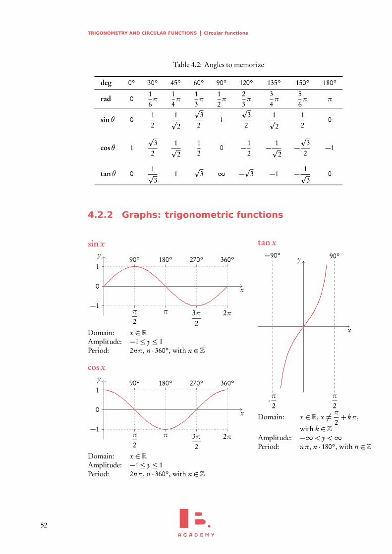
Table 4.2: Angles to memorize
deg 0° 30° 45° 60° 90° 120° 135° 150° 180°
rad 016π
14π
13π
12π
23π
34π
56π π
sinθ 012
1p
2
p3
21
p3
21p
2
12
0
cosθ 1
p3
21p
2
12
0 −12
− 1p
2−p
32
−1
tanθ 01p
31
p3 ∞ −
p3 −1 − 1
p3
0
4.2.2 Graphs: trigonometric functions
sin x
x
y
π
2
90°
π
180°
3π2
270°
2π
360°
−1
1
0
Domain: x ∈RAmplitude: −1≤ y ≤ 1Period: 2nπ, n · 360°, with n ∈Z
cos x
x
y
π
2
90°
π
180°
3π2
270°
2π
360°
−1
1
0
Domain: x ∈RAmplitude: −1≤ y ≤ 1Period: 2nπ, n · 360°, with n ∈Z
tan x
x
y
-π
2
−90°
π
2
90°
Domain: x ∈R, x 6= π2+ kπ,
with k ∈ZAmplitude: −∞< y <∞Period: nπ, n · 180°, with n ∈Z
52
TRIGONOMETRY AND CIRCULAR FUNCTIONS Circular functions 4
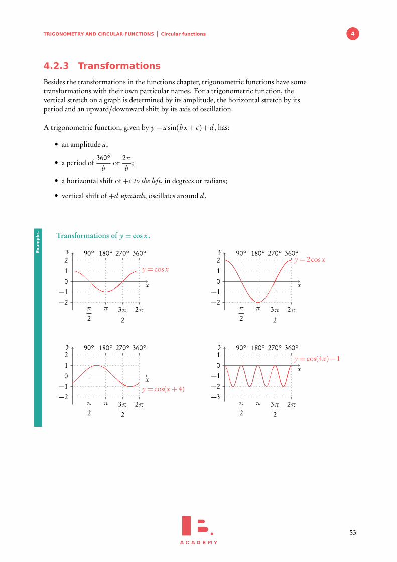
4.2.3 Transformations
Besides the transformations in the functions chapter, trigonometric functions have sometransformations with their own particular names. For a trigonometric function, thevertical stretch on a graph is determined by its amplitude, the horizontal stretch by itsperiod and an upward/downward shift by its axis of oscillation.
A trigonometric function, given by y = a sin(b x + c)+ d , has:
• an amplitude a;
• a period of360°
bor
2πb
;
• a horizontal shift of +c to the left, in degrees or radians;
• vertical shift of +d upwards, oscillates around d .
Transformations of y = cos x .
x
y
π
2
90°
π
180°
3π2
270°
2π
360°
−2−1
12
0
y = cos x
x
y
π
2
90°
π
180°
3π2
270°
2π
360°
−2−1
12
0
y = 2cos x
x
y
π
2
90°
π
180°
3π2
270°
2π
360°
−2−1
12
0
y = cos(x + 4)
x
y
π
2
90°
π
180°
3π2
270°
2π
360°
−3−2−1
10
y = cos(4x)− 1
Exam
ple.
53
TRIGONOMETRY AND CIRCULAR FUNCTIONS Circular functions
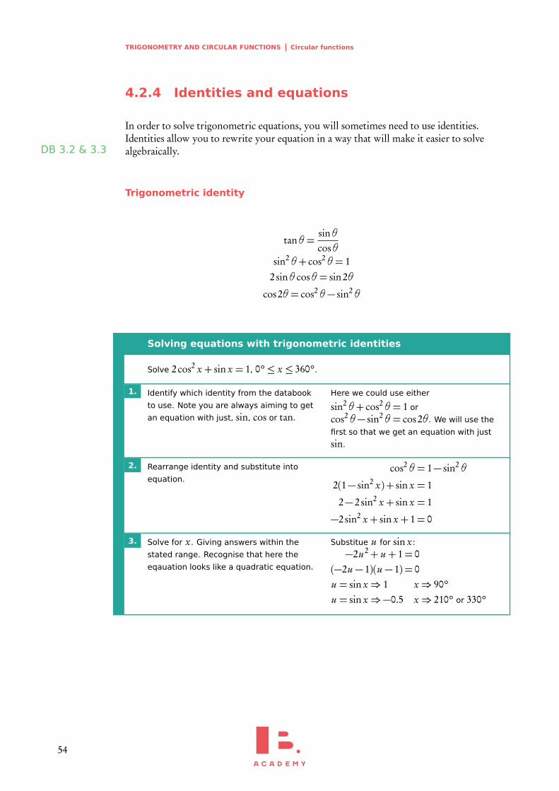
4.2.4 Identities and equations
In order to solve trigonometric equations, you will sometimes need to use identities.Identities allow you to rewrite your equation in a way that will make it easier to solvealgebraically.DB 3.2 & 3.3
Trigonometric identity
tanθ=sinθcosθ
sin2θ+ cos2θ= 12sinθ cosθ= sin2θ
cos2θ= cos2θ− sin2θ
Solving equations with trigonometric identities
Solve 2cos2 x + sin x = 1, 0°≤ x ≤ 360°.
1. Identify which identity from the databook
to use. Note you are always aiming to get
an equation with just, sin, cos or tan.
Here we could use either
sin2θ+ cos2θ= 1 or
cos2θ− sin2θ= cos2θ. We will use the
first so that we get an equation with just
sin.
2. Rearrange identity and substitute into
equation.cos2θ= 1− sin2θ
2(1− sin2 x)+ sin x = 1
2− 2sin2 x + sin x = 1
−2sin2 x + sin x + 1= 0
3. Solve for x . Giving answers within the
stated range. Recognise that here the
eqauation looks like a quadratic equation.
Substitue u for sin x:
−2u2+ u + 1= 0(−2u − 1)(u − 1) = 0u = sin x⇒ 1 x⇒ 90°u = sin x⇒−0.5 x⇒ 210° or 330°
54

TRIGONOMETRY AND CIRCULAR FUNCTIONS Circular functions 4
Double angle and half angle formulae
sin (A±B) = sinAcosB ± cosAsinBcos (A±B) = cosAcosB ± sinAsinB
tan (A±B) =tanA± tanB
1± tanAtanBcos (2a) = cos2 a− sin2 a = 2cos2 a− 1= 1− 2sin2 asin (2a) = 2sina cosa
tan (2a) =2tana
1− tan2 a
From the double angle we can obtain half angles.
cosa = cos2�a
2
�
− sin2�a
2
�
= 2cos2�a
2
�
− 1= 1− 2sin2�a
2
�
sina = 2sin�a
2
�
cos�a
2
�
tana =2tan
�a2
�
1− tan2�a
2
�
4.2.5 Inverse and reciprocal trigonometric
functionsDB
Inverse trigonometric functions
The inverse of a trigonometric function is useful for finding an angle. You should alreadybe familiar with carrying this operation out on a calculator.
sinθ=π
2⇒ θ= arcsin
π
2
Just like the inverse functions, trigonometric inverse functions have the property thatthe range of the original function is its domain and vice versa.
55

TRIGONOMETRY AND CIRCULAR FUNCTIONS Circular functions
sin−1 x = arcsin x
x
y
−1 0 1
−90°
90°
Domain: −1≤ x ≤ 1Range: −π
2≤ y ≤ π
2
cos−1 x = arccos x
x
y
−1 0 1
180°
Domain: −1≤ x ≤ 1Range: 0≤ y ≤π
tan−1 x = arctan x
x
y
−10−9−8−7−6−5−4−3−2−1 0 1 2 3 4 5 6 7 8 9 10
−90°
90°
Domain: x ∈RRange: −π
2≤ y ≤ π
2
56

TRIGONOMETRY AND CIRCULAR FUNCTIONS Circular functions 4
Reciprocal trigonometric functions
1sinθ
= cscθ
x
y
−180° 180° 360°−1
1
1cosθ
= secθ
x
y
−90° 90° 270°−1
1
1tanθ
= cotθ
x
y
−180° 180° 360°
These functions are the reciprocal functions, their vertical asyptotes correspond to thex-axis intercepts of the original function. The functions cscθ and secθ are periodic witha period of 360°, cotθ has a period of 180°.
57

5DIFFERENTIATIONTable of contents & cheatsheet
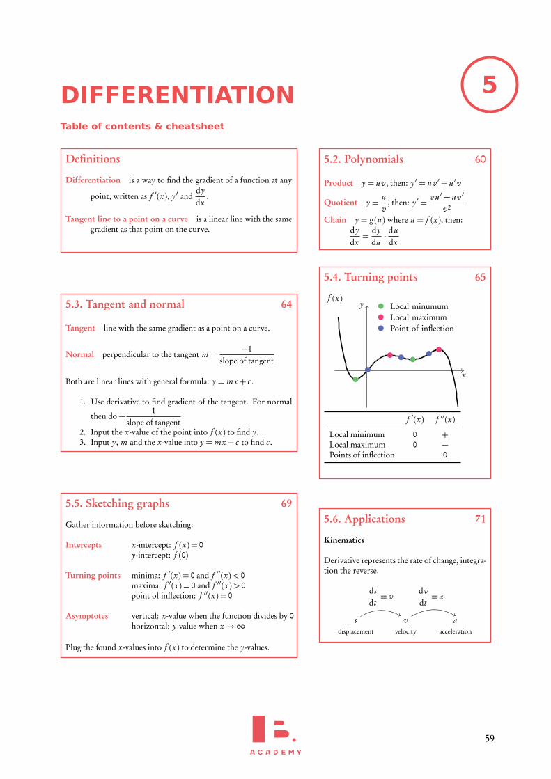
Definitions
Differentiation is a way to find the gradient of a function at any
point, written as f ′(x), y ′ anddydx
.
Tangent line to a point on a curve is a linear line with the samegradient as that point on the curve.
5.2. Polynomials 60
Product y = uv, then: y ′ = uv ′+ u ′v
Quotient y =uv
, then: y ′ =v u ′− uv ′
v2
Chain y = g (u) where u = f (x), then:dydx=
dydu· du
dx
5.3. Tangent and normal 64
Tangent line with the same gradient as a point on a curve.
Normal perpendicular to the tangent m =−1
slope of tangent
Both are linear lines with general formula: y = mx + c .
1. Use derivative to find gradient of the tangent. For normal
then do − 1slope of tangent
.
2. Input the x-value of the point into f (x) to find y.3. Input y, m and the x-value into y = mx + c to find c .
5.4. Turning points 65
x
yf (x)
Local minumumLocal maximumPoint of inflection
f ′(x) f ′′(x)
Local minimum 0 +Local maximum 0 −Points of inflection 0
5.5. Sketching graphs 69
Gather information before sketching:
Intercepts x-intercept: f (x) = 0y-intercept: f (0)
Turning points minima: f ′(x) = 0 and f ′′(x)< 0maxima: f ′(x) = 0 and f ′′(x)> 0point of inflection: f ′′(x) = 0
Asymptotes vertical: x-value when the function divides by 0horizontal: y-value when x→∞
Plug the found x-values into f (x) to determine the y-values.
5.6. Applications 71
Kinematics
Derivative represents the rate of change, integra-tion the reverse.
s v adisplacement velocity acceleration
d sdt= v
dvdt= a
59

DIFFERENTIATION Derivation from first principles
5.1 Derivation from first principles
As the derivative at a point is the gradient, differentiation can be compared to finding
gradients of lines: m =y2− y1
x2− x1.
x
f (x)
x + h
f (x + h)
h
Using the graph
x1 = x x2 = x + hy1 = f (x) y2 = f (x + h)
Plugging into the equation of the gradient of a line
m =f (x + h)− f (x)
x + h − x
Taking the limit of h going to zero, such that the distance between the points becomesvery small, one can approximate the gradient at a point of any funtion:
f ′(x) = limh→0
f (x + h)− f (x)h
5.2 Polynomials
As you have learnt in the section on functions, a straight line graph has a gradient. Thisgradient describes the rate at which the graph is changing and thanks to it we can tellhow steep the line will be. In fact gradients can be found for any function - the specialthing about linear functions is that their gradient is always the same (given by min y = mx + c ). For polynomial functions the gradient is always changing. This is wherecalculus comes in handy; we can use differentiation to derive a function using which wecan find the gradient for any value of x.
Using the following steps, you can find the derivative function ( f ′(x)) for anypolynomial function ( f (x)).
60
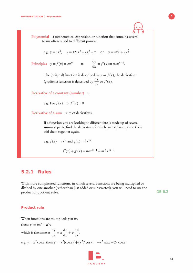
DIFFERENTIATION Polynomials 5
Polynomial a mathematical expression or function that contains severalterms often raised to different powers
e.g. y = 3x2, y = 121x5+ 7x3+ x or y = 4x23 + 2x
13
Principles y = f (x) = axn ⇒dydx= f ′(x) = naxn−1.
The (original) function is described by y or f (x), the derivative
(gradient) function is described bydydx
or f ′(x).
Derivative of a constant (number) 0
e.g. For f (x) = 5, f ′(x) = 0
Derivative of a sum sum of derivatives.
If a function you are looking to differentiate is made up of severalsummed parts, find the derivatives for each part separately and thenadd them together again.
e.g. f (x) = axn and g (x) = b x m
f ′(x)+ g ′(x) = naxn−1+mb x m−1
5.2.1 Rules
With more complicated functions, in which several functions are being multiplied ordivided by one another (rather than just added or substracted), you will need to use theproduct or quotient rules. DB 6.2
Product rule
When functions are multiplied: y = uv
then: y ′ = uv ′+ u ′v
which is the same asdydx= u
dvdx+ v
dudx
.
e.g. y = x2 cos x, then y ′ = x2(cos x)′+(x2)′ cos x =−x2 sin x + 2x cos x
61
DIFFERENTIATION Polynomials
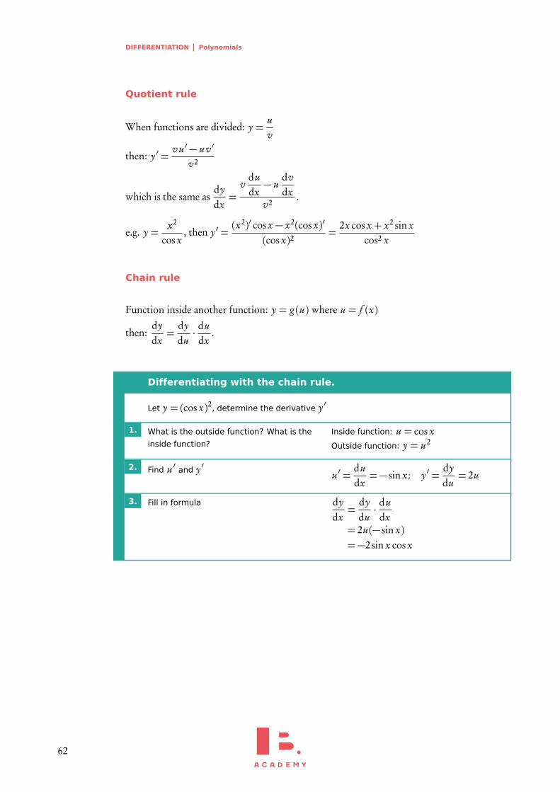
Quotient rule
When functions are divided: y =uv
then: y ′ =v u ′− uv ′
v2
which is the same asdydx=
vdudx− u
dvdx
v2.
e.g. y =x2
cos x, then y ′ =
(x2)′ cos x − x2(cos x)′
(cos x)2=
2x cos x + x2 sin xcos2 x
Chain rule
Function inside another function: y = g (u) where u = f (x)
then:dydx=
dydu· du
dx.
Differentiating with the chain rule.
Let y = (cos x)2, determine the derivative y ′
1. What is the outside function? What is the
inside function?
Inside function: u = cos xOutside function: y = u2
2. Find u ′ and y ′ u ′ =dudx=− sin x; y ′ =
dydu= 2u
3. Fill in formula dydx=
dydu· du
dx= 2u(− sin x)=−2sin x cos x
62

DIFFERENTIATION Polynomials 5
5.2.2 Implicit differentiation
When we have a function that does not express y explicitely (y =) like in the previousmethods, we must use implicit differentiation.
Steps to follow:
1. differentiate with respect to x, don’t forget chain and x rules. Derivative of y isdydx
2. collect/gather terms withdydx
3. solve fordydx
Implicit differentiation
Find the gradient at point (0,1) of exy + ln�
y2�
+ ey = 1+ e
1. Treat each part seperatelyexy becomes yexy +
dydx
xexy
ln�
y2�
becomes 2y +1y2
dydx=
2y
xdydx
ey becomesdydx
ey
2.Collect/gather terms with
dydx
yexy +dydx
xexy +dydx
2y+
dydx
ey = 0
dydx
�
xexy +2y+ ey
�
=−yexy
dydx=
−yexy
xexy +2y+ ey
3. Solve for the point (0,1) Substituting in x = 0 and y = 1dydx=−1
2+ e
63
DIFFERENTIATION Tangent and normal equation
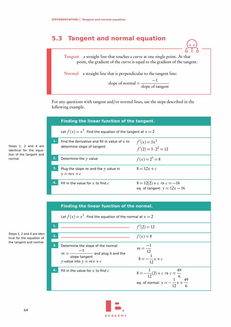
5.3 Tangent and normal equation
Tangent a straight line that touches a curve at one single point. At thatpoint, the gradient of the curve is equal to the gradient of the tangent.
Normal a straight line that is perpendicular to the tangent line:
slope of normal=−1
slope of tangent
For any questions with tangent and/or normal lines, use the steps described in thefollowing example.
Finding the linear function of the tangent.
Let f (x) = x3. Find the equation of the tangent at x = 2
1. Find the derivative and fill in value of x to
determine slope of tangentSteps 1, 2 and 4 areidentical for the equa-tion of the tangent andnormal
f ′(x) = 3x2
f ′(2) = 3 · 22 = 12
2. Determine the y value f (x) = 23 = 8
3. Plug the slope m and the y value in
y = mx + c8= 12x + c
4. Fill in the value for x to find c 8= 12(2)+ c ⇒ c =−16eq. of tangent: y = 12x − 16
Finding the linear function of the normal.
Let f (x) = x3. Find the equation of the normal at x = 2
1. f ′(2) = 12
Steps 1, 2 and 4 are iden-tical for the equation ofthe tangent and normal
2. f (x) = 8
3. Determine the slope of the normal
m =−1
slope tangentand plug it and the
y-value into y = mx + c
m =−112
8=− 112
x + c
4. Fill in the value for x to find c 8=− 112(2)+ c ⇒ c =
496
eq. of normal: y =− 112
x +496
64

DIFFERENTIATION Turning points 5
To find the gradient of a function for any value of x .
f (x) = 5x3− 2x2+ x. Find the gradient of f (x) at x = 3.
IB ACADEMY
Press menu
4: Calculus
1: Numerical Derivative
at a Point
IB ACADEMY
Enter the variable used inyour function (x) and thevalue of x that you want tofind. Keep the settings on1st Derivative
Press OK
IB ACADEMY
Type in your function
press≈
enter
In this case, f ′(3) = 124
5.4 Turning points
There are three types of turning points:
1. Local maxima
2. Local minima
3. Points of inflection
We know that when f ′(x) = 0 there will be a maximum or a minimum. Whether it is amaximum or minimum should be evident from looking at the graph of the originalfunction. If a graph is not available, we can find out by plugging in a slightly smaller andslightly larger value than the point in question into f ′(x). If the smaller value is negativeand the larger value positive then it is a local minimum. If the smaller value is positiveand the larger value negative then it is a local minimum.
If you take the derivative of a derivative function (one you have already derived) you getthe second derivate. In mathematical notation, the second derivative is written as y ′′,
f ′′(x) ord2ydx2
. We can use this to determine whether a point on a graph is a maximum, a
minimum or a point of inflection as demonstrated in the following Figure 5.1.
65
DIFFERENTIATION Turning points
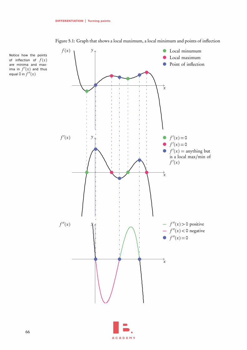
Figure 5.1: Graph that shows a local maximum, a local minimum and points of inflection
Notice how the points
of inflection of f (x)are minima and max-ima in f ′(x) and thus
equal 0 in f ′′(x)
x
y
x
y
x
y
f (x)
f ′(x)
f ′′(x)
Local minumumLocal maximumPoint of inflection
f ′(x) = 0f ′(x) = 0f ′(x) = anything butis a local max/min off ′(x)
f ′′(x) = 0
f ′′(x)> 0 positivef ′′(x)< 0 negative
66
DIFFERENTIATION Turning points 5
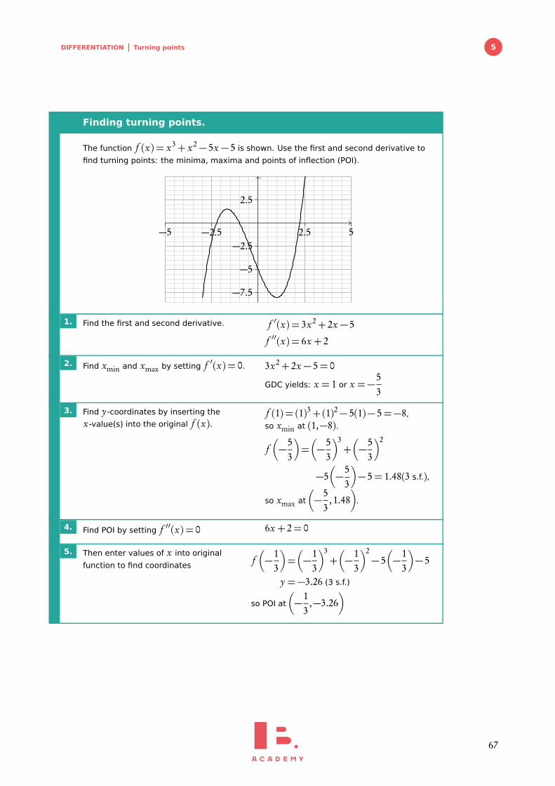
Finding turning points.
The function f (x) = x3+ x2− 5x − 5 is shown. Use the first and second derivative to
find turning points: the minima, maxima and points of inflection (POI).
−5 −2.5 2.5 5
−7.5
−5
−2.5
2.5
1. Find the first and second derivative. f ′(x) = 3x2+ 2x − 5
f ′′(x) = 6x + 2
2. Find xmin and xmax by setting f ′(x) = 0. 3x2+ 2x − 5= 0
GDC yields: x = 1 or x =−53
3. Find y-coordinates by inserting the
x-value(s) into the original f (x).f (1) = (1)3+(1)2− 5(1)− 5=−8,
so xmin at (1,−8).
f�
−53
�
=�
−53
�3+�
−53
�2
−5�
−53
�
− 5= 1.48(3 s.f.),
so xmax at
�
−53
,1.48�
.
4. Find POI by setting f ′′(x) = 0 6x + 2= 0
5. Then enter values of x into original
function to find coordinates f�
−13
�
=�
−13
�3+�
−13
�2− 5
�
−13
�
− 5
y =−3.26 (3 s.f.)
so POI at
�
−13
,−3.26�
67

DIFFERENTIATION Turning points
To find turning points (local maximum/minimum) of a function
Find the coordinates of the local minimum for f (x) = 4x2− 5x + 3
IB ACADEMY
Press menu
6: Analyze graph
or 2: Minimum
or 3: Maximum
IB ACADEMY
Use the cursor to set thebounds (the min/maxmust be between thebounds)
IB ACADEMY
So the coordinates of theminimum for f (x) are(0.625,1.44)
68
DIFFERENTIATION Sketching graphs 5
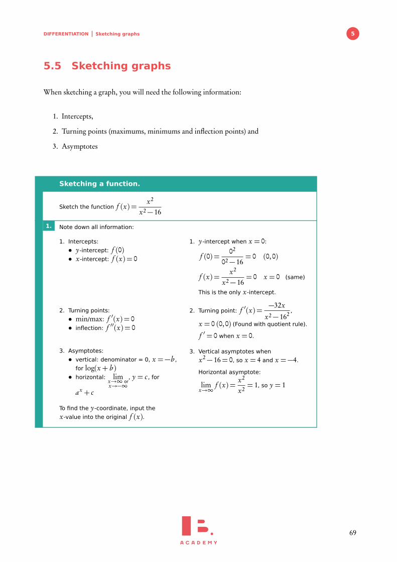
5.5 Sketching graphs
When sketching a graph, you will need the following information:
1. Intercepts,
2. Turning points (maximums, minimums and inflection points) and
3. Asymptotes
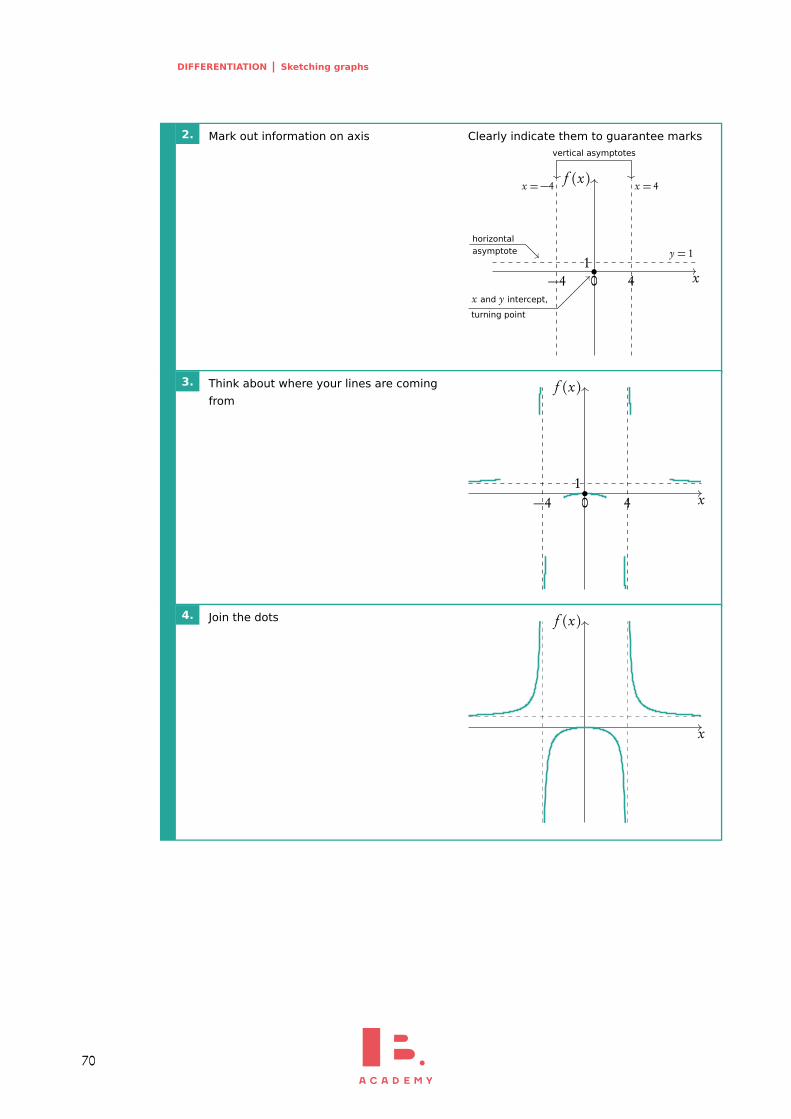
Sketching a function.
Sketch the function f (x) =x2
x2− 16
1. Note down all information:
1. Intercepts:
• y-intercept: f (0)• x-intercept: f (x) = 0
2. Turning points:
• min/max: f ′(x) = 0• inflection: f ′′(x) = 0
3. Asymptotes:
• vertical: denominator = 0, x =−b ,
for log(x + b )• horizontal: lim
x→∞ orx→−∞
, y = c , for
ax + c
To find the y-coordinate, input the
x-value into the original f (x).
1. y-intercept when x = 0:
f (0) =02
02− 16= 0 (0,0)
f (x) =x2
x2− 16= 0 x = 0 (same)
This is the only x-intercept.
2. Turning point: f ′(x) =−32x
x2− 162 ,
x = 0 (0,0) (Found with quotient rule).
f ′ = 0 when x = 0.
3. Vertical asymptotes when
x2− 16= 0, so x = 4 and x =−4.
Horizontal asymptote:
limx→∞
f (x) =x2
x2= 1, so y = 1
69
DIFFERENTIATION Sketching graphs
2. Mark out information on axis Clearly indicate them to guarantee marks
x
f (x)
x and y intercept,
turning point
x =−4 x = 4
y = 1
vertical asymptotes
horizontalasymptote
−4 0 41
3. Think about where your lines are coming
from
x
f (x)
−4 0 41
4. Join the dots
x
f (x)
70

DIFFERENTIATION Applications 5
5.6 Applications
5.6.1 Kinematics
Kinematics deals with the movement of bodies over time. When you are given onefunction to calculate displacement, velocity or acceleration you can use differentiation orintegration to determine the functions for the other two.
Displacement, s
Velocity, v =d sdt
Acceleration,
a =dvdt=
d2 sdt 2
d sdt
dvdt
∫
a dt
∫
v dt
The derivative represents the rate of change, i.e. the gradient of a graph. So, velocity isthe rate of change in displacement and acceleration is the rate of change in velocity.
Answering kinematics questions.
A diver jumps from a platform at time t = 0 seconds. The distance of the diver above
water level at time t is given by s(t ) =−4.9t 2+ 4.9t + 10, where s is in metres.
Find when velocity equals zero. Hence find the maximum height of the diver.
1. Find an equation for velocity by
differentiating equation for distance
v(t ) =−9.8t + 4.9
2. Solve for v(t ) = 0 −9.8t + 4.9= 0, t = 0.5
3. Put value into equation for distance to
find height above waters(0.5) =−4.9(0.5)2+ 4.9(0.5)+ 10=11.225m
71
DIFFERENTIATION Applications
5.6.2 Optimization
We can use differentiation to find minimum and maximum areas/volumes of variousshapes. Often the key skill with these questions is to find an expression using simplegeometric formulas and rearranging in order to differentiate.
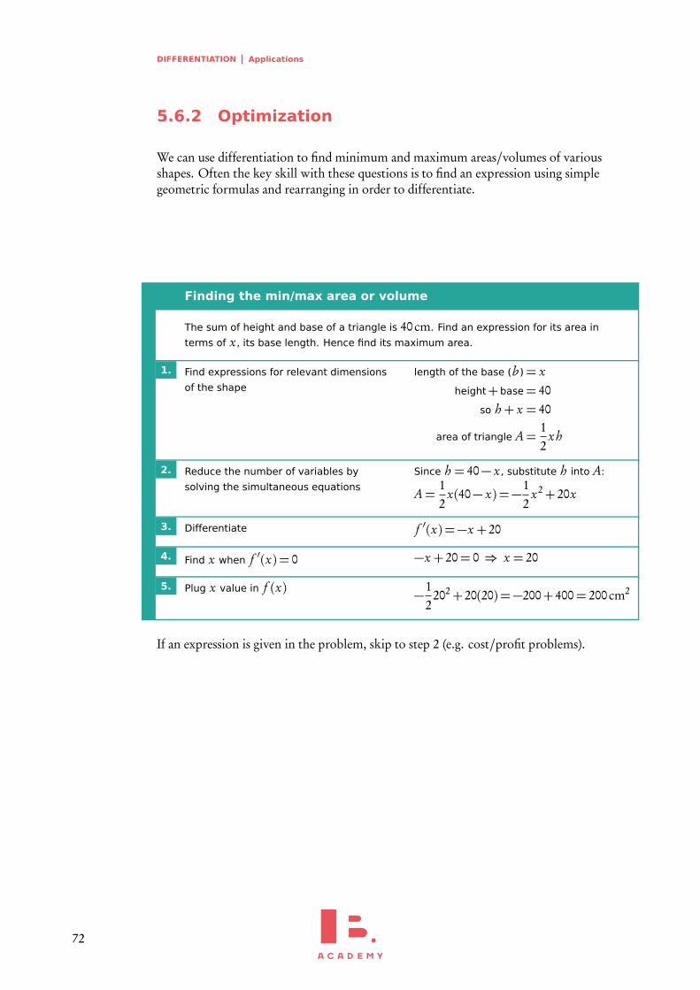
Finding the min/max area or volume
The sum of height and base of a triangle is 40cm. Find an expression for its area in
terms of x , its base length. Hence find its maximum area.
1. Find expressions for relevant dimensions
of the shape
length of the base (b )= xheight+ base= 40
so h + x = 40
area of triangle A=12
x h
2. Reduce the number of variables by
solving the simultaneous equations
Since h = 40− x , substitute h into A:
A=12
x(40− x) =−12
x2+ 20x
3. Differentiate f ′(x) =−x + 20
4. Find x when f ′(x) = 0 −x + 20= 0 ⇒ x = 20
5. Plug x value in f (x) −12
202+ 20(20) =−200+ 400= 200cm2
If an expression is given in the problem, skip to step 2 (e.g. cost/profit problems).
72
DIFFERENTIATION Implicit differentiation 5
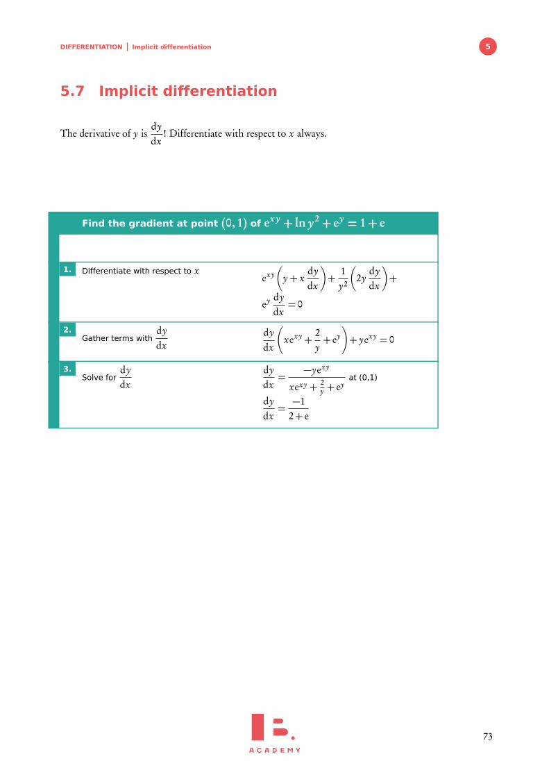
5.7 Implicit differentiation
The derivative of y isdydx
! Differentiate with respect to x always.
Find the gradient at point (0, 1) of exy + ln y2+ ey = 1+ e
1. Differentiate with respect to xexy
�
y + xdydx
�
+1y2
�
2ydydx
�
+
ey dydx= 0
2.Gather terms with
dydx
dydx
�
xexy +2y+ ey
�
+ yexy = 0
3.Solve for
dydx
dydx=
−yexy
xexy + 2y + ey
at (0,1)
dydx=−1
2+ e
73


6INTEGRATIONTable of contents & cheatsheet
6.1. Indefinite integral 76
∫
xn dx =xn+1
n+ 1+C n 6=−1
Integration with an internal function∫
f (ax + b )dx
Integrate normally and multiply by1
coefficient of x
Integration by substitution∫
f�
g (x)�
· g ′(x)dx
6.2. Definite integral 78
∫ b
af (x)dx = F (b )− F (a) where F =
∫
f (x)dx
Be careful, the order you substitute a and b into theindefinite integral is relevant for your answer:
∫ b
af (x)dx =−
∫ a
bf (x)dx
Area between a curve and the x-axis
By determining a definite integral for a function, you can findthe area beneath the curve that is between the two x-valuesindicated as its limits.
Acurve =∫ b
af (x)dx
x
y
a b
f (x)
Note: the area below the x-axis gives a negative valuefor its area. You must take that value as a positive valueto determine the area between a curve and the x-axis.Sketching the graph will show what part of the functionlies below the x-axis.
Area between two curves
Using definite integrals you can also find the areas enclosedbetween curves.
Abetween =∫ b
a
�
g (x)− f (x)�
dxx
y
a b
f (x)
g (x)
With g (x) as the “top” function (furthest from the x-axis). For the area between curves, it does not matterwhat is above/below the x-axis.
Volume of revolution
V =π∫ b
ay2 dx =
∫ b
aπy2 dx
Besides finding areas under and between curves, integra-tion can also be used to calculate the volume of the solidthat a curve would make if it were rotated 360° aroundits axis - this is called the volume of revolution.
75
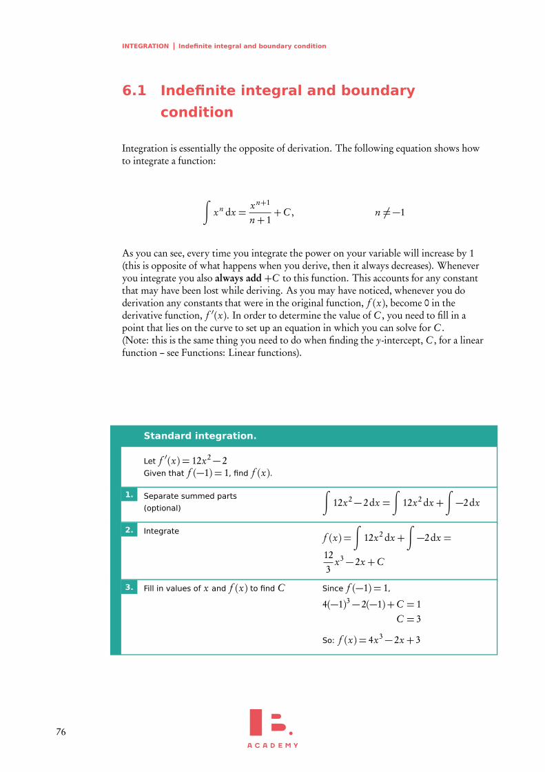
INTEGRATION Indefinite integral and boundary condition
6.1 Indefinite integral and boundary
condition
Integration is essentially the opposite of derivation. The following equation shows howto integrate a function:
∫
xn dx =xn+1
n+ 1+C , n 6=−1
As you can see, every time you integrate the power on your variable will increase by 1(this is opposite of what happens when you derive, then it always decreases). Wheneveryou integrate you also always add +C to this function. This accounts for any constantthat may have been lost while deriving. As you may have noticed, whenever you doderivation any constants that were in the original function, f (x), become 0 in thederivative function, f ′(x). In order to determine the value of C , you need to fill in apoint that lies on the curve to set up an equation in which you can solve for C .(Note: this is the same thing you need to do when finding the y-intercept, C , for a linearfunction – see Functions: Linear functions).
Standard integration.
Let f ′(x) = 12x2− 2Given that f (−1) = 1, find f (x).
1. Separate summed parts
(optional)
∫
12x2− 2dx =∫
12x2 dx +∫
−2dx
2. Integratef (x) =
∫
12x2 dx +∫
−2dx =
123
x3− 2x +C
3. Fill in values of x and f (x) to find C Since f (−1) = 1,
4(−1)3− 2(−1)+C = 1C = 3
So: f (x) = 4x3− 2x + 3
76
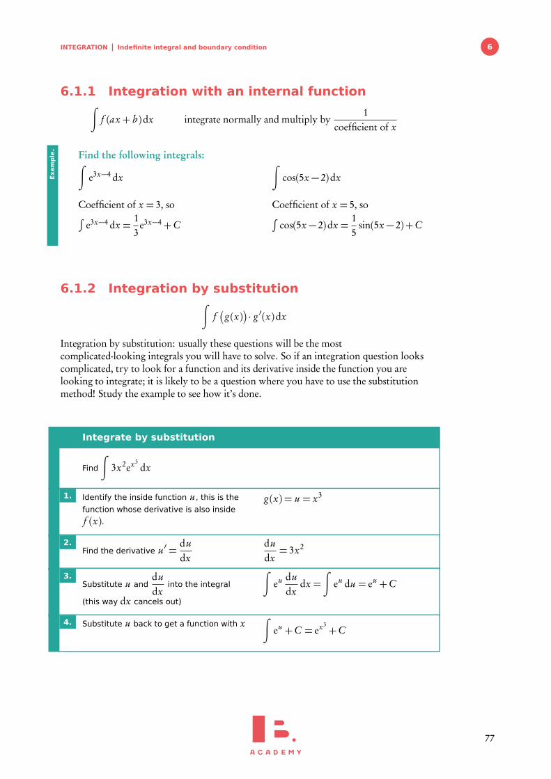
INTEGRATION Indefinite integral and boundary condition 6
6.1.1 Integration with an internal function∫
f (ax + b )dx integrate normally and multiply by1
coefficient of x
Find the following integrals:∫
e3x−4 dx
Coefficient of x = 3, so∫
e3x−4 dx =13
e3x−4+C
∫
cos(5x − 2)dx
Coefficient of x = 5, so∫
cos(5x − 2)dx =15
sin(5x − 2)+C
Exam
ple.
6.1.2 Integration by substitution∫
f�
g (x)�
· g ′(x)dx
Integration by substitution: usually these questions will be the mostcomplicated-looking integrals you will have to solve. So if an integration question lookscomplicated, try to look for a function and its derivative inside the function you arelooking to integrate; it is likely to be a question where you have to use the substitutionmethod! Study the example to see how it’s done.
Integrate by substitution
Find
∫
3x2ex3dx
1. Identify the inside function u , this is the
function whose derivative is also inside
f (x).
g (x) = u = x3
2.Find the derivative u ′ =
dudx
dudx= 3x2
3.Substitute u and
dudx
into the integral
(this way dx cancels out)
∫
eu dudx
dx =∫
eu du = eu +C
4. Substitute u back to get a function with x∫
eu +C = ex3+C
77

INTEGRATION Definite integral
6.2 Definite integral
If there are limit values indicated on your integral, you are looking to find a definiteintegral. This means that these values will be used to find a numeric answer rather than afunction.
This is done in the following way, where the values for a and b are substituted as x-valuesinto your indefinite integral:
∫ b
af (x)dx = F (b )− F (a) where F =
∫
f (x)dx
Be careful, the order you substitute a and b into the indefinite integral is relevant foryour answer:
∫ b
af (x)dx =−
∫ a
bf (x)dx
Solving definite integrals.
Find
∫ 7
312x2− 2dx , knowing that F (x) = 4x3− 2x
1. Find the indefinite integral
(without +C )
∫ 7
312x2− 2dx =
�
4x3− 2x�7
3
2. Fill in: F (b )− F (a)(integral x = b )− (integral x = a)
=�
4(7)3− 2(7)�
−�
4(3)3− 2(3)�
= 1256
78
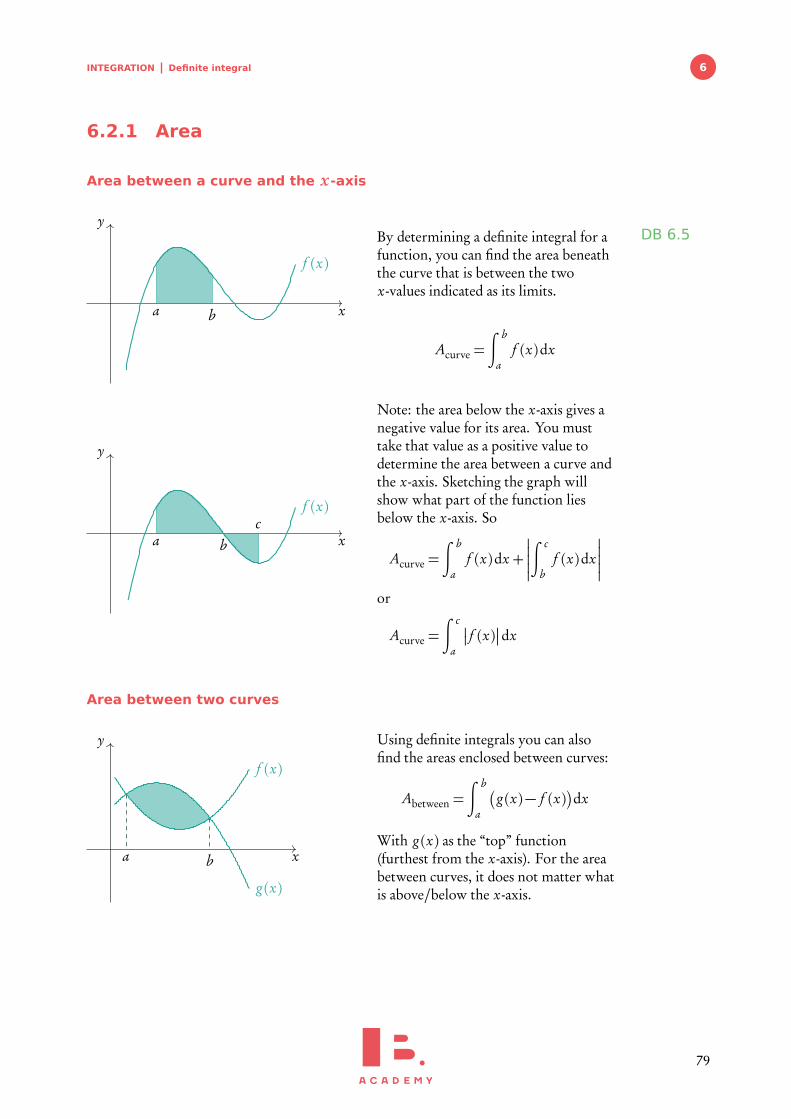
INTEGRATION Definite integral 6
6.2.1 Area
Area between a curve and the x-axis
x
y
a b
f (x)
DB 6.5By determining a definite integral for afunction, you can find the area beneaththe curve that is between the twox-values indicated as its limits.
Acurve =∫ b
af (x)dx
x
y
a bc
f (x)
Note: the area below the x-axis gives anegative value for its area. You musttake that value as a positive value todetermine the area between a curve andthe x-axis. Sketching the graph willshow what part of the function liesbelow the x-axis. So
Acurve =∫ b
af (x)dx +
�
�
�
�
�
∫ c
bf (x)dx
�
�
�
�
�
or
Acurve =∫ c
a
�
� f (x)�
�dx
Area between two curves
x
y
a b
f (x)
g (x)
Using definite integrals you can alsofind the areas enclosed between curves:
Abetween =∫ b
a
�
g (x)− f (x)�
dx
With g (x) as the “top” function(furthest from the x-axis). For the areabetween curves, it does not matter whatis above/below the x-axis.
79
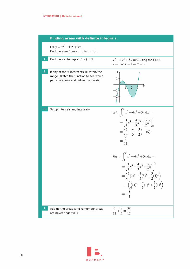
INTEGRATION Definite integral
Finding areas with definite integrals.
Let y = x3− 4x2+ 3xFind the area from x = 0 to x = 3.
1. Find the x-intercepts: f (x) = 0 x3− 4x2+ 3x = 0, using the GDC:
x = 0 or x = 1 or x = 3
2. If any of the x-intercepts lie within the
range, sketch the function to see which
parts lie above and below the x-axis.
x
y
1 2 3
−2
−1
1
3. Setup integrals and integrateLeft:
∫ 1
0x3− 4x2+ 3x dx =
=�
14
x4− 43
x3+32
x2�1
0
=�
14− 4
3+
32
�
− (0)
=512
Right:
∫ 3
1x3− 4x2+ 3x dx =
=�
14
x4− 43
x3+32
x2�3
1
=�
14(3)4− 4
3(3)3+
32(3)2
�
−�
14(1)4− 4
3(1)3+
32(1)2
�
=−83
4. Add up the areas (and remember areas
are never negative!)
512+
83=
3712
80
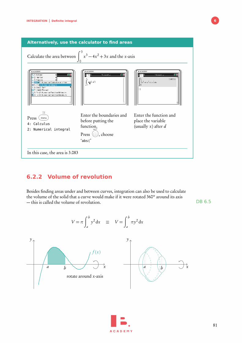
INTEGRATION Definite integral 6
Alternatively, use the calculator to find areas
Calculate the area between∫ 3
0x3− 4x2+ 3x and the x-axis
IB ACADEMY
Press menu
4: Calculus
2: Numerical integral
IB ACADEMY
Enter the boundaries andbefore putting thefunction.
Press∞β◦
, choose‘abs(’
IB ACADEMY
Enter the function andplace the variable(usually x) after d
In this case, the area is 3.083
6.2.2 Volume of revolution
Besides finding areas under and between curves, integration can also be used to calculatethe volume of the solid that a curve would make if it were rotated 360° around its axis— this is called the volume of revolution. DB 6.5
V =π∫ b
ay2 dx ≡ V =
∫ b
aπy2 dx
x
rotate around x-axis
y
a b
f (x)
x
y
a b
81
INTEGRATION Definite integral
Find the area from x = 1 to x = 4 for the function y =p
x .
A=∫ 4
1
px dx =
�
23
x32
�4
1=�
23(4)
32
�
−�
23(1)
32
�
=143
This area is rotated 360° (= 2π) around the x -axis. Find the volume of the solid.
V =π∫ 4
1
px2 dx =π
∫ 4
1x dx =π
�
12
x2�4
1=π
�
�
12(4)2
�
−�
12(1)2
�
�
=15π
2
Exam
ple.
6.2.3 Integration by partsDB
General statement:∫
u · dv = uv −∫
v · du or∫
f (x)g ′(x)dx = f g −∫
f ′ g dx
Solve∫
x sin x dxIf f (x) = x then f ′(x) = 1 and the derivative of g (x) =−cos x is g ′(x) = sin x
−x cos x −∫
1 · sin x dx =−x cos x + cos x +C
Exam
ple.
Sometimes it may be necessary to do intergration by parts multiple times.
Solve∫
e2x sin x dxWe know that sin x is the derivative of cos x
u = sin x du = cos x dx
dv = e2x dx v =e2x
2
Using the formula given in the data booklet and the information above:∫
e2x sin x dx =e2x sin x
2−∫
e2x
2cos x dx
Unfortunately this is still not nice to solve so we need to repeat the procedure along
the same line of reasoning for the integral∫
e2x
2cos x dx.
We know trigonometric functions recur – taking the integral twice would bring usback to the same trigonometric identity, apart from containing the opposite sign.
Exam
ple.
82
INTEGRATION Definite integral 6
u = cos x du =− sin x dx
dv =e2x
2dx v =
e2x
4
We again construct the formula of integration by parts.∫
e2x
2cos x dx = cos x
e2x
4−∫
e2x
4sin x dx
Now we want to combine both equations to solve for the original integral.∫
e2x sin x dx =e2x sin x
2− cos x
e2x
4+∫
e2x
4sin x dx
54
∫
e2x sin x dx =e2x sin x
2− cos x
e2x
4
=25
sin xe2x − 15
cos xe2x
Exam
ple.
83

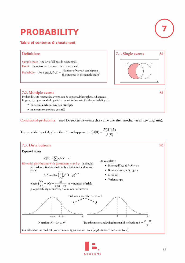
7PROBABILITYTable of contents & cheatsheet
Definitions
Sample space the list of all possible outcomes.
Event the outcomes that meet the requirement.
Probability for event A, P (A) =Number of ways A can happen
all outcomes in the sample space.
7.1. Single events 86
A B
0
7.2. Multiple events 88Probabilities for successive events can be expressed through tree diagrams.In general, if you are dealing with a question that asks for the probability of:
• one event and another, you multiply
• one event or another, you add
Conditional probability used for successive events that come one after another (as in tree diagrams).
The probability of A, given that B has happened: P (A|B) =P (A∩B)
P (B).
7.3. Distributions 90
Expected values
E(X ) =∑
xP (X = x)
Binomial distribution with parameters n and p it shouldbe used for situations with only 2 outcomes and lots oftrials
P (X = x) =�
nr
�
p r �1− p�n−r
where�
nr
�
= nCr=n!
r !(n− r )!, n = number of trials,
p = probability of success, r = number of success.
On calculator:
• Binompdf(n,p,r) P (X = r )
• Binomcdf(n,p,r) P (x ≤ r )
• Mean np
• Varience npq
xmean St. dv.
Notation: X ∼N (µ,σ2)
z0 1
Transform to standardised normal distribution: Z =x −µσ
total area under the curve = 1
On calculator: normal cdf (lower bound, upper bound, mean (=µ), standard deviation (= σ ))
85
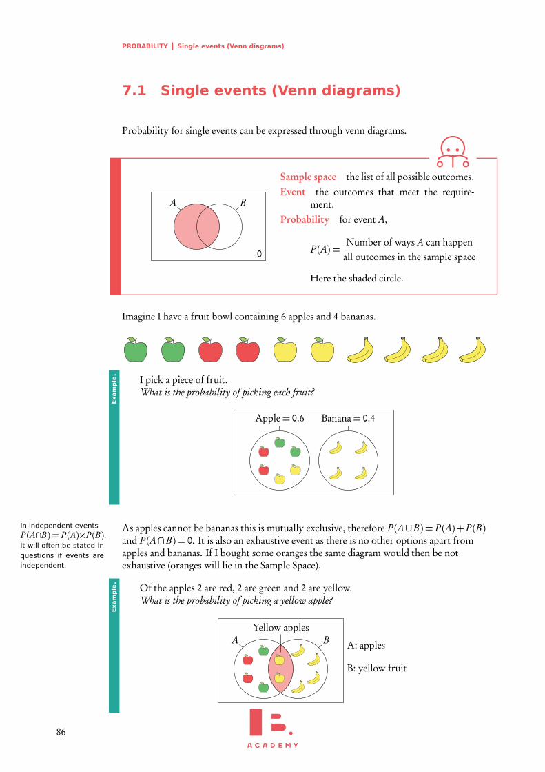
PROBABILITY Single events (Venn diagrams)
7.1 Single events (Venn diagrams)
Probability for single events can be expressed through venn diagrams.
A B
0
Sample space the list of all possible outcomes.Event the outcomes that meet the require-
ment.Probability for event A,
P (A) =Number of ways A can happen
all outcomes in the sample space
Here the shaded circle.
Imagine I have a fruit bowl containing 6 apples and 4 bananas.
I pick a piece of fruit.What is the probability of picking each fruit?
Apple= 0.6 Banana= 0.4
Exam
ple.
In independent eventsP (A∩B) = P (A)×P (B).It will often be stated inquestions if events areindependent.
As apples cannot be bananas this is mutually exclusive, therefore P (A∪B) = P (A)+ P (B)and P (A∩B) = 0. It is also an exhaustive event as there is no other options apart fromapples and bananas. If I bought some oranges the same diagram would then be notexhaustive (oranges will lie in the Sample Space).
Of the apples 2 are red, 2 are green and 2 are yellow.What is the probability of picking a yellow apple?
A BYellow apples
A: apples
B: yellow fruit
Exam
ple.
86
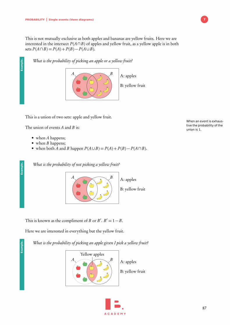
PROBABILITY Single events (Venn diagrams) 7
This is not mutually exclusive as both apples and bananas are yellow fruits. Here we areinterested in the intersect P (A∩B) of apples and yellow fruit, as a yellow apple is in bothsets P (A∩B) = P (A)+ P (B)− P (A∪B).
What is the probability of picking an apple or a yellow fruit?
A B A: apples
B: yellow fruit
Exam
ple.
This is a union of two sets: apple and yellow fruit.When an event is exhaus-tive the probability of theunion is 1.
The union of events A and B is:
• when A happens;• when B happens;• when both A and B happen P (A∪B) = P (A)+ P (B)− P (A∩B).
What is the probability of not picking a yellow fruit?
A B A: apples
B: yellow fruit
Exam
ple.
This is known as the compliment of B or B ′. B ′ = 1−B .
Here we are interested in everything but the yellow fruit.
What is the probability of picking an apple given I pick a yellow fruit?
A BYellow apples
A: apples
B: yellow fruit
Exam
ple.
87
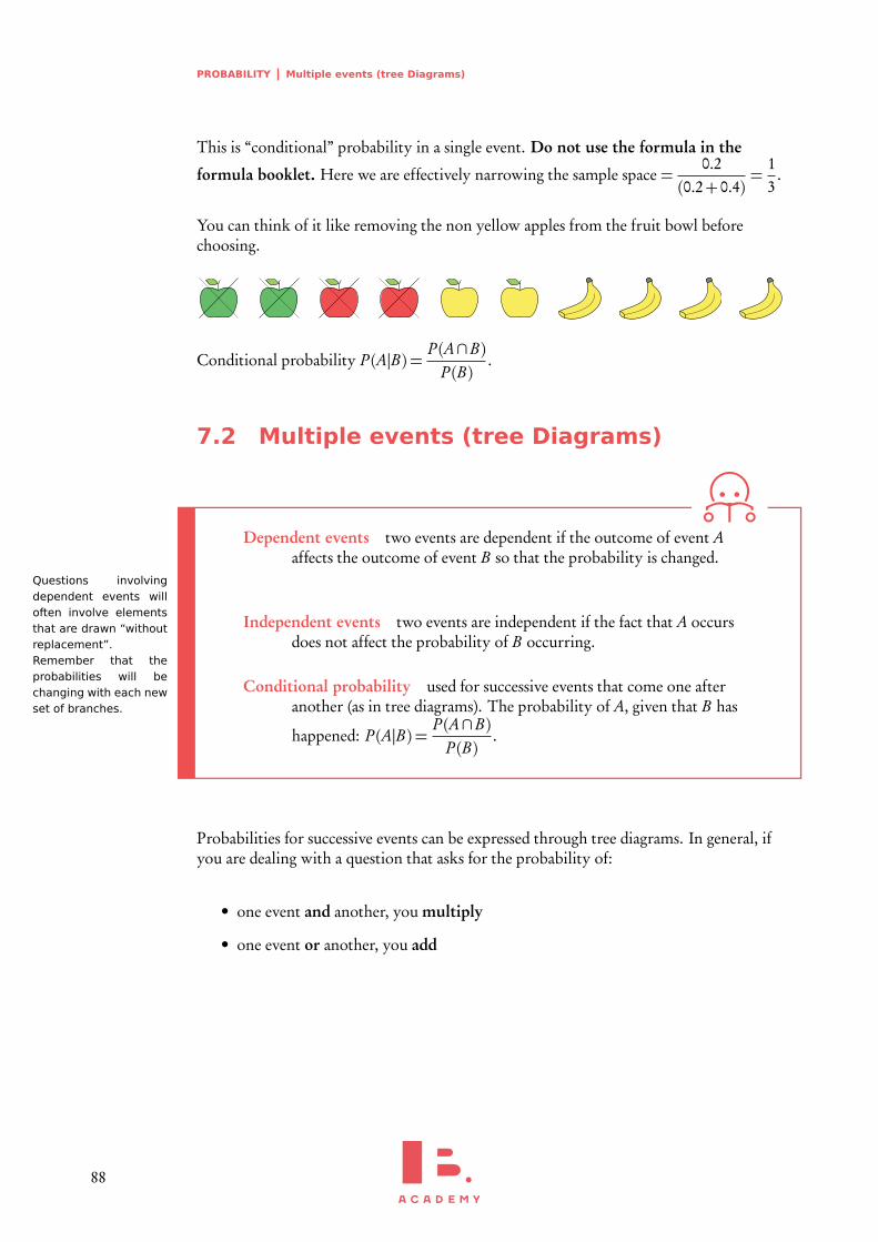
PROBABILITY Multiple events (tree Diagrams)
This is “conditional” probability in a single event. Do not use the formula in the
formula booklet. Here we are effectively narrowing the sample space =0.2
(0.2+ 0.4)=
13
.
You can think of it like removing the non yellow apples from the fruit bowl beforechoosing.
Conditional probability P (A|B) =P (A∩B)
P (B).
7.2 Multiple events (tree Diagrams)
Dependent events two events are dependent if the outcome of event Aaffects the outcome of event B so that the probability is changed.
Questions involvingdependent events willoften involve elementsthat are drawn “withoutreplacement”.Remember that theprobabilities will bechanging with each newset of branches.
Independent events two events are independent if the fact that A occursdoes not affect the probability of B occurring.
Conditional probability used for successive events that come one afteranother (as in tree diagrams). The probability of A, given that B has
happened: P (A|B) =P (A∩B)
P (B).
Probabilities for successive events can be expressed through tree diagrams. In general, ifyou are dealing with a question that asks for the probability of:
• one event and another, you multiply
• one event or another, you add
88
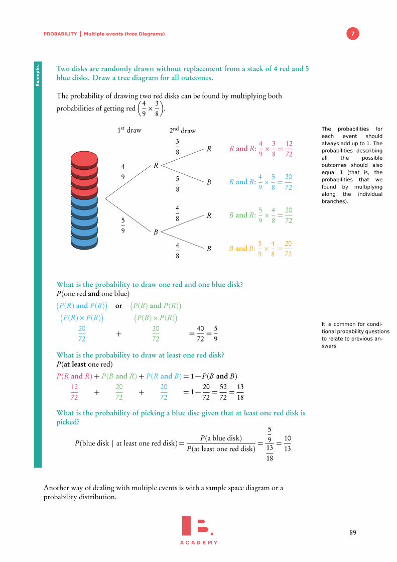
PROBABILITY Multiple events (tree Diagrams) 7
Two disks are randomly drawn without replacement from a stack of 4 red and 5blue disks. Draw a tree diagram for all outcomes.
The probability of drawing two red disks can be found by multiplying both
probabilities of getting red�
49× 3
8
�
.
The probabilities foreach event shouldalways add up to 1. Theprobabilities describingall the possibleoutcomes should alsoequal 1 (that is, theprobabilities that wefound by multiplyingalong the individualbranches).
R
B
R
B
R
B
49
59
38
58
48
48
1st draw 2nd draw
R and R:49× 3
8=
1272
R and B :49× 5
8=
2072
B and R:59× 4
8=
2072
B and B :59× 4
8=
2072
What is the probability to draw one red and one blue disk?P (one red and one blue)�
P (R) and P (B)�
or�
P (B) and P (R)�
�
P (R)× P (B)� �
P (B)× P (R)�
2072
+2072
=4072=
59
It is common for condi-tional probability questionsto relate to previous an-swers.
What is the probability to draw at least one red disk?P (at least one red)
P (R and R) + P (B and R) + P (R and B) = 1− P (B and B)1272
+2072
+2072
= 1− 2072=
5272=
1318
What is the probability of picking a blue disc given that at least one red disk ispicked?
P (blue disk | at least one red disk) =P (a blue disk)
P (at least one red disk)=
591318
=1013
Exam
ple.
Another way of dealing with multiple events is with a sample space diagram or aprobability distribution.
89
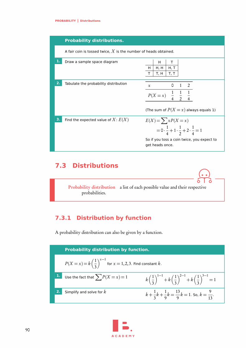
PROBABILITY Distributions
Probability distributions.
A fair coin is tossed twice, X is the number of heads obtained.
1. Draw a sample space diagram H T
H H, H H, T
T T, H T, T
2. Tabulate the probability distribution x 0 1 2
P (X = x)14
12
14
(The sum of P (X = x) always equals 1)
3. Find the expected value of X : E(X ) E(X ) =∑
xP (X = x)
= 0 · 14+ 1 · 1
2+ 2 · 1
4= 1
So if you toss a coin twice, you expect to
get heads once.
7.3 Distributions
Probability distribution a list of each possible value and their respectiveprobabilities.
7.3.1 Distribution by function
A probability distribution can also be given by a function.
Probability distribution by function.
P (X = x) = k�
13
�x−1for x = 1,2,3. Find constant k .
1. Use the fact that∑
P (X = x) = 1 k�
13
�1−1+ k
�
13
�2−1+ k
�
13
�3−1= 1
2. Simplify and solve for k k +13
k +19
k =139
k = 1. So, k =913
.
90
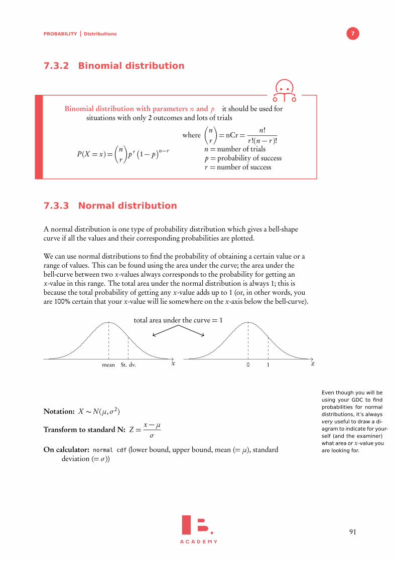
PROBABILITY Distributions 7
7.3.2 Binomial distribution
Binomial distribution with parameters n and p it should be used forsituations with only 2 outcomes and lots of trials
P (X = x) =�
nr
�
p r �1− p�n−r
where�
nr
�
= nCr=n!
r !(n− r )!n = number of trialsp = probability of successr = number of success
7.3.3 Normal distribution
A normal distribution is one type of probability distribution which gives a bell-shapecurve if all the values and their corresponding probabilities are plotted.
We can use normal distributions to find the probability of obtaining a certain value or arange of values. This can be found using the area under the curve; the area under thebell-curve between two x-values always corresponds to the probability for getting anx-value in this range. The total area under the normal distribution is always 1; this isbecause the total probability of getting any x-value adds up to 1 (or, in other words, youare 100% certain that your x-value will lie somewhere on the x-axis below the bell-curve).
xmean St. dv. z0 1
total area under the curve = 1
Even though you will beusing your GDC to findprobabilities for normaldistributions, it’s alwaysvery useful to draw a di-agram to indicate for your-self (and the examiner)what area or x-value youare looking for.
Notation: X ∼N (µ,σ2)
Transform to standard N: Z =x −µσ
On calculator: normal cdf (lower bound, upper bound, mean (=µ), standarddeviation (= σ ))
91
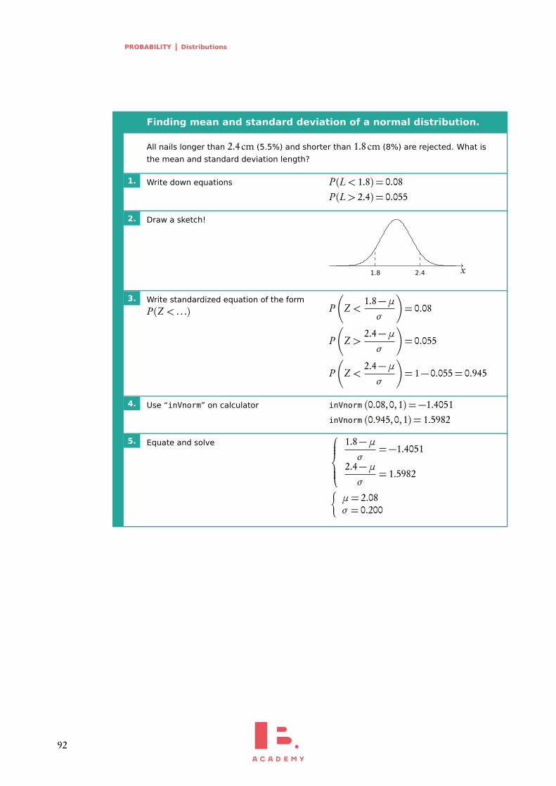
PROBABILITY Distributions
Finding mean and standard deviation of a normal distribution.
All nails longer than 2.4 cm (5.5%) and shorter than 1.8 cm (8%) are rejected. What is
the mean and standard deviation length?
1. Write down equations P (L< 1.8) = 0.08P (L> 2.4) = 0.055
2. Draw a sketch!
x1.8 2.4
3. Write standardized equation of the form
P (Z < . . .) P
�
Z <1.8−µσ
�
= 0.08
P
�
Z >2.4−µσ
�
= 0.055
P
�
Z <2.4−µσ
�
= 1− 0.055= 0.945
4. Use “inVnorm” on calculator inVnorm (0.08,0,1) =−1.4051inVnorm (0.945,0,1) = 1.5982
5. Equate and solve
1.8−µσ
=−1.4051
2.4−µσ
= 1.5982�
µ= 2.08σ = 0.200
92
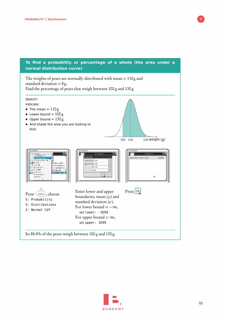
PROBABILITY Distributions 7
To find a probability or percentage of a whole (the area under a
normal distribution curve)
The weights of pears are normally distributed with mean= 110g andstandard deviation= 8g.Find the percentage of pears that weigh between 100 g and 130 g
Sketch!
Indicate:
• The mean = 110g• Lower bound = 100g• Upper bound = 130g• And shade the area you are looking to
find.
weight (g)100 110 130
IB ACADEMY
Press menu , choose5: Probability
5: Distributions
2: Normal Cdf
IB ACADEMY
Enter lower and upperboundaries, mean (µ) andstandard deviation (σ ).For lower bound = −∞,
set lower: -1E99
For upper bound =∞,set upper: 1E99
IB ACADEMY
Press OK
So 88.8% of the pears weigh between 100 g and 130 g.
93
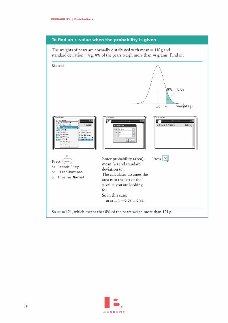
PROBABILITY Distributions
To find an x-value when the probability is given
The weights of pears are normally distributed with mean= 110g andstandard deviation= 8g. 8% of the pears weigh more than m grams. Find m.
Sketch!
weight (g)110 m
8%= 0.08
IB ACADEMY
Press menu
5: Probability
5: Distributions
3: Inverse Normal
IB ACADEMY
Enter probability (Area),mean (µ) and standarddeviation (σ ).The calculator assumes thearea is to the left of thex-value you are lookingfor.So in this case:
area= 1− 0.08= 0.92
IB ACADEMY
Press OK
So m = 121, which means that 8% of the pears weigh more than 121 g.
94
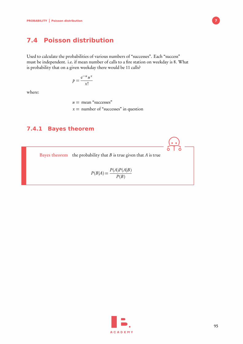
PROBABILITY Poisson distribution 7
7.4 Poisson distribution
Used to calculate the probabilities of various numbers of “successes”. Each “success”must be independent. i.e. if mean number of calls to a fire station on weekday is 8. Whatis probability that on a given weekday there would be 11 calls?
p =e−u u x
x!
where:
u = mean “successes”x = number of “successes” in question
7.4.1 Bayes theorem
Bayes theorem the probability that B is true given that A is true
P (B |A) =P (A)P (A|B)
P (B)
95

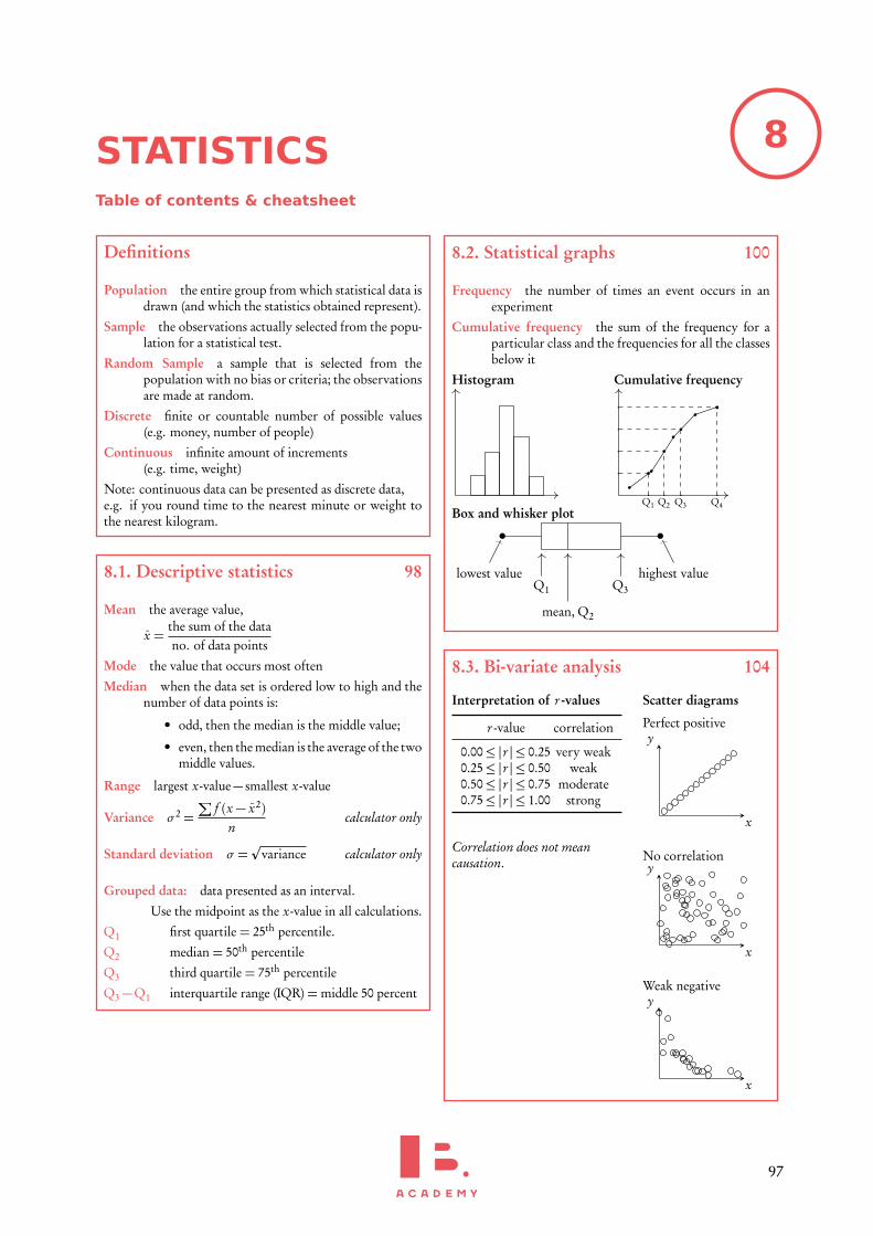
8STATISTICSTable of contents & cheatsheet
Definitions
Population the entire group from which statistical data isdrawn (and which the statistics obtained represent).
Sample the observations actually selected from the popu-lation for a statistical test.
Random Sample a sample that is selected from thepopulation with no bias or criteria; the observationsare made at random.
Discrete finite or countable number of possible values(e.g. money, number of people)
Continuous infinite amount of increments(e.g. time, weight)
Note: continuous data can be presented as discrete data,e.g. if you round time to the nearest minute or weight tothe nearest kilogram.
8.1. Descriptive statistics 98
Mean the average value,
x =the sum of the datano. of data points
Mode the value that occurs most often
Median when the data set is ordered low to high and thenumber of data points is:
• odd, then the median is the middle value;
• even, then the median is the average of the twomiddle values.
Range largest x-value− smallest x-value
Variance σ2 =∑
f (x − x2)n
calculator only
Standard deviation σ =p
variance calculator only
Grouped data: data presented as an interval.
Use the midpoint as the x-value in all calculations.
Q1 first quartile = 25th percentile.
Q2 median = 50th percentile
Q3 third quartile = 75th percentile
Q3−Q1 interquartile range (IQR) =middle 50 percent
8.2. Statistical graphs 100
Frequency the number of times an event occurs in anexperiment
Cumulative frequency the sum of the frequency for aparticular class and the frequencies for all the classesbelow it
Histogram Cumulative frequency
Q1 Q2 Q3 Q4Box and whisker plot
lowest valueQ1
mean, Q2
Q3
highest value
8.3. Bi-variate analysis 104
Interpretation of r -values
r -value correlation
0.00≤ |r | ≤ 0.25 very weak0.25≤ |r | ≤ 0.50 weak0.50≤ |r | ≤ 0.75 moderate0.75≤ |r | ≤ 1.00 strong
Correlation does not meancausation.
Scatter diagrams
Perfect positive
x
y
No correlation
x
y
Weak negative
x
y
97

STATISTICS Descriptive statistics
8.1 Descriptive statistics
The mean, mode and median, are all ways of measuring “averages”. Depending on thedistribution of the data, the values for the mean, mode and median can differ slightly or alot. Therefore, the mean, mode and median are all useful for understanding your data set.
Example data set: 6, 3, 6, 13, 7, 7 in a table:x 3 6 7 13frequency 1 2 2 1
Mean the average value, x =the sum of the datano. of data points
=∑
xn=∑
f x∑
fMode the value that occurs most often (highest frequency)
Median the middle value when the data set is ordered low to high. Evennumber of values: the median is the average of the two middle values.
Find for larger values as n+12
.
Range largest x-value− smallest x-value
Variance σ2 =∑
f (x − x2)n
calculator only
Standard deviation σ =p
variance calculator only
Note on grouped data: data presented as an interval; e.g. 10–20 cm.
• Use the midpoint as the x-value in all calculations. So for 10–20 cm use15 cm.
• For 10–20 cm, 10 is the lower boundary, 20 is the upper boundary andthe width is 20− 10= 10.
Adding a constant to all the values in a data set or multiplying the entire data set by aconstant influences the mean and standard deviation values in the following way:
Table 8.1: Adding or multiplying by a constant
adding constant k multiplying by kmean x + k k × xstandard deviation σ k ×σ
98

STATISTICS Descriptive statistics 8
Q1 first quartile = 25th percentile.The value for x so that 25% of all the data values are ≤ to it.
Q2 median = 50th percentile
Q3 third quartile = 75th percentile
Q3−Q1 interquartile range (IQR) =middle 50 percent
Snow depth is measured in centimeters:30, 75, 125, 55, 60, 75, 65, 65, 45, 120, 70, 110.Find the range, the median, the lower quartile, the upper quartile and theinterquartile range.
First always rearrange data into ascending order: 30,45,55,60,65,65,70,75,75,110,120,125
1. The range:125− 30= 95cm
2. The median: there are 12 values so the median is between the 6th and 7th value.
65+ 702
= 67.5cm
3. The lower quartile: there are 12 values so the lower quartile is between the 3rd
and 4th value.55+ 60
2= 57.5cm
4. The upper quartile: there are 12 values so the lower quartile is between the 9th
and 10th value.75+ 110
2= 92.5cm
5. The IQR92.5− 57.5= 35cm
Exam
ple.
99

STATISTICS Statistical graphs
8.2 Statistical graphs
Frequency the number of times an event occurs in an experiment
Cumulative frequency the sum of the frequency for a particular class andthe frequencies for all the classes below it
Age 17 18 19 20 21No. of students 21 45 93 61 20Cumulative freq. 21 66 159 220 240
Age
f
17 18 19 20 21
102030405060708090
100A histogram is used to display the frequency for a specificcondition. The frequencies (here: # of students) aredisplayed on the y-axis, and the different classes of thesample (here: age) are displayed on the x-axis. As such,the differences in frequency between the different classesassumed in the sample can easily be compared.
Age
cf
17 18 19 20 21
50
100
150
200
250
Q1 Q2 Q3 Q4
The cumulative frequency graph is used to display thedevelopment of the frequencies as the classes of the eventincrease. The graph is plotted by using the sum of allfrequencies for a particular class, added to the frequenciesfor all the classes below it. The classes of the event (age)are displayed on the x-axis, and the frequency isdisplayed on the y-axis. The cumulative frequency graphalways goes upwards, because the cumulative frequencyincreases as you include more classes.
lowest valueQ1 Q2 Q3
highest value
Box and whisker plots neatly summarizethe distribution of the data. It givesinformation about the range, the medianand the quartiles of the data. The firstand third quartiles are at the ends of thebox, the median is indicated with avertical line in the interior of the box,and the maximum and minimum pointsare at the ends of the whiskers.
100
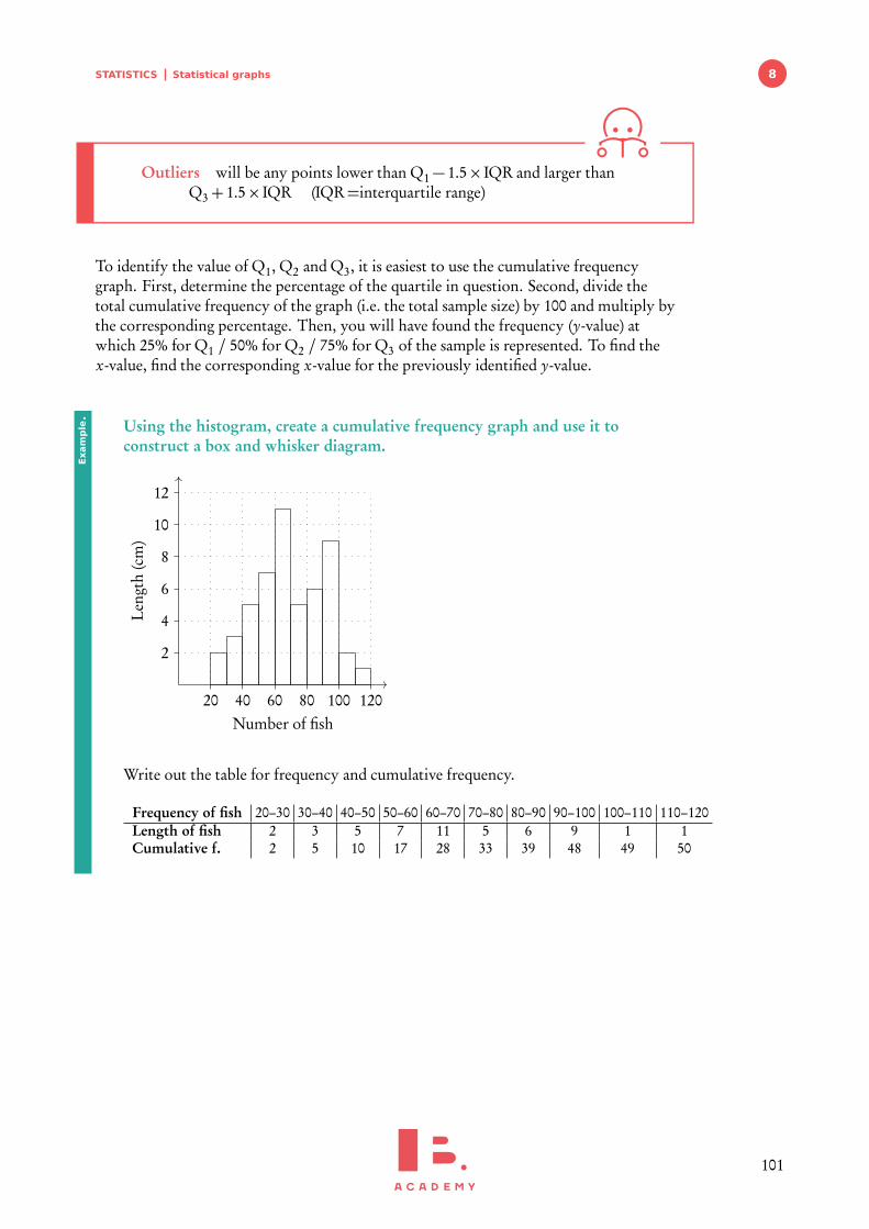
STATISTICS Statistical graphs 8
Outliers will be any points lower than Q1− 1.5× IQR and larger thanQ3+ 1.5× IQR (IQR=interquartile range)
To identify the value of Q1, Q2 and Q3, it is easiest to use the cumulative frequencygraph. First, determine the percentage of the quartile in question. Second, divide thetotal cumulative frequency of the graph (i.e. the total sample size) by 100 and multiply bythe corresponding percentage. Then, you will have found the frequency (y-value) atwhich 25% for Q1 / 50% for Q2 / 75% for Q3 of the sample is represented. To find thex-value, find the corresponding x-value for the previously identified y-value.
Using the histogram, create a cumulative frequency graph and use it toconstruct a box and whisker diagram.
Number of fish
Leng
th(c
m)
20 40 60 80 100 120
2
4
6
8
10
12
Write out the table for frequency and cumulative frequency.
Frequency of fish 20–30 30–40 40–50 50–60 60–70 70–80 80–90 90–100 100–110 110–120Length of fish 2 3 5 7 11 5 6 9 1 1Cumulative f. 2 5 10 17 28 33 39 48 49 50
Exam
ple.
101
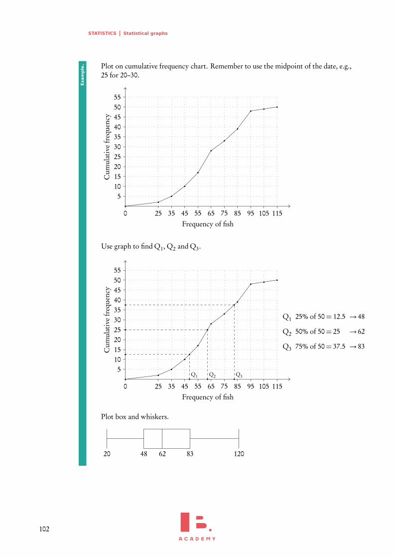
STATISTICS Statistical graphs
Plot on cumulative frequency chart. Remember to use the midpoint of the date, e.g.,25 for 20–30.
Frequency of fish
Cum
ulat
ive
freq
uenc
y
0 25 35 45 55 65 75 85 95 105 115
510152025303540455055
Use graph to find Q1, Q2 and Q3.
Frequency of fish
Cum
ulat
ive
freq
uenc
y
0 25 35 45 55 65 75 85 95 105 115
510152025303540455055
Q1 Q2 Q3
Q1 25% of 50= 12.5 → 48
Q2 50% of 50= 25 → 62
Q3 75% of 50= 37.5 → 83
Plot box and whiskers.
20 1206248 83
Exam
ple.
102
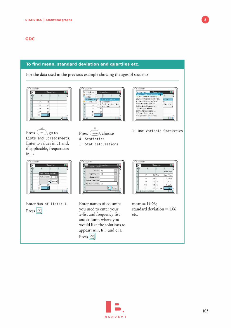
STATISTICS Statistical graphs 8
GDC
To find mean, standard deviation and quartiles etc.
For the data used in the previous example showing the ages of students
IB ACADEMY
Pressoff
on , go toLists and Spreadsheets.Enter x-values in L1 and,if applicable, frequenciesin L2
IB ACADEMY
Press menu , choose4: Statistics
1: Stat Calculations
IB ACADEMY
1: One-Variable Statistics
IB ACADEMY
Enter Num of lists: 1.
Press OK
IB ACADEMY
Enter names of columnsyou used to enter yourx-list and frequency listand column where youwould like the solutions toappear: a[], b[] and c[].
Press OK
IB ACADEMY
mean= 19.06;standard deviation= 1.06etc.
103
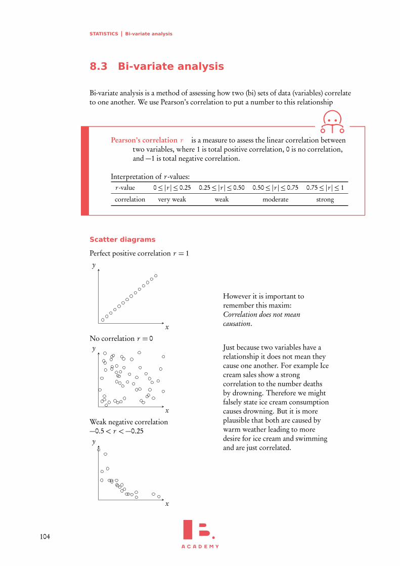
STATISTICS Bi-variate analysis
8.3 Bi-variate analysis
Bi-variate analysis is a method of assessing how two (bi) sets of data (variables) correlateto one another. We use Pearson’s correlation to put a number to this relationship
Pearson’s correlation r is a measure to assess the linear correlation betweentwo variables, where 1 is total positive correlation, 0 is no correlation,and −1 is total negative correlation.
Interpretation of r -values:r -value 0≤ |r | ≤ 0.25 0.25≤ |r | ≤ 0.50 0.50≤ |r | ≤ 0.75 0.75≤ |r | ≤ 1
correlation very weak weak moderate strong
Scatter diagrams
Perfect positive correlation r = 1
x
y
No correlation r = 0
x
y
Weak negative correlation−0.5< r <−0.25
x
y
However it is important toremember this maxim:Correlation does not meancausation.
Just because two variables have arelationship it does not mean theycause one another. For example Icecream sales show a strongcorrelation to the number deathsby drowning. Therefore we mightfalsely state ice cream consumptioncauses drowning. But it is moreplausible that both are caused bywarm weather leading to moredesire for ice cream and swimmingand are just correlated.
104
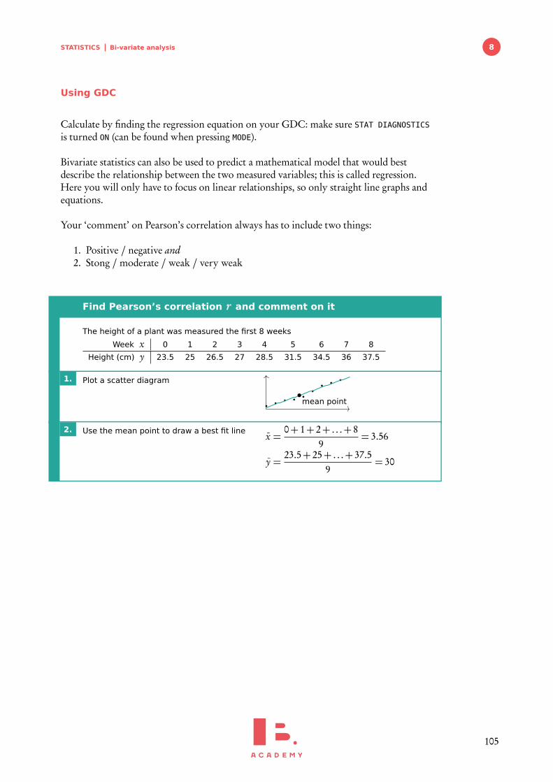
STATISTICS Bi-variate analysis 8
Using GDC
Calculate by finding the regression equation on your GDC: make sure STAT DIAGNOSTICS
is turned ON (can be found when pressing MODE).
Bivariate statistics can also be used to predict a mathematical model that would bestdescribe the relationship between the two measured variables; this is called regression.Here you will only have to focus on linear relationships, so only straight line graphs andequations.
Your ‘comment’ on Pearson’s correlation always has to include two things:
1. Positive / negative and2. Stong /moderate / weak / very weak
Find Pearson’s correlation r and comment on it
The height of a plant was measured the first 8 weeks
Week x 0 1 2 3 4 5 6 7 8
Height (cm) y 23.5 25 26.5 27 28.5 31.5 34.5 36 37.5
1. Plot a scatter diagram
mean point
2. Use the mean point to draw a best fit line x =0+ 1+ 2+ . . .+ 8
9= 3.56
y =23.5+ 25+ . . .+ 37.5
9= 30
105
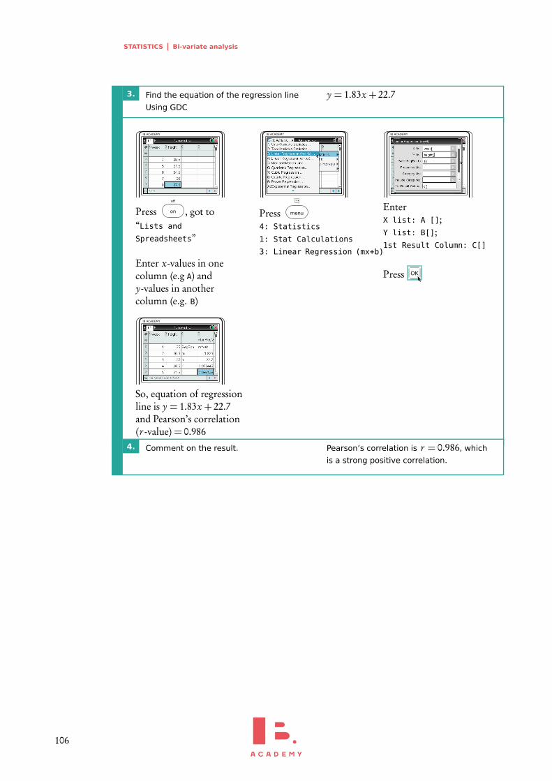
STATISTICS Bi-variate analysis
3. Find the equation of the regression line
Using GDC
y = 1.83x + 22.7
IB ACADEMY
Pressoff
on , got to“Lists and
Spreadsheets”
Enter x-values in onecolumn (e.g A) andy-values in anothercolumn (e.g. B)
IB ACADEMY
Press menu
4: Statistics
1: Stat Calculations
3: Linear Regression (mx+b)
IB ACADEMY
EnterX list: A [];Y list: B[];1st Result Column: C[]
Press OK
IB ACADEMY
So, equation of regressionline is y = 1.83x + 22.7and Pearson’s correlation(r -value) = 0.986
4. Comment on the result. Pearson’s correlation is r = 0.986, which
is a strong positive correlation.
106