Localization in inelastic rate dependent

shearing deformations

Theodoros Katsaounis∗† Min-Gi Lee∗ Athanasios Tzavaras∗‡§

Abstract

Metals deformed at high strain rates can exhibit failure through formation of shearbands, a phenomenon often attributed to Hadamard instability and localization of thestrain into an emerging coherent structure. We verify formation of shear bands for anonlinear model exhibiting strain softening and strain rate sensitivity. The effects ofstrain softening and strain rate sensitivity are first assessed by linearized analysis, in-dicating that the combined effect leads to Turing instability. For the nonlinear modela class of self-similar solutions is constructed, that depicts a coherent localizing struc-ture and the formation of a shear band. This solution is associated to a heteroclinicorbit of a dynamical system. The orbit is constructed numerically and yields explicitshear localizing solutions.

1 Introduction

Shear bands are narrow zones of intense shear observed during the dynamic deformationof many metals at high strain rates. Shear localization forms a striking instance ofmaterial instability, often preceding rupture, and its study has attracted considerableattention in the mechanics e.g. [8, 11, 16, 1, 25, 7, 22, 5, 24], numerical [23, 6, 10], ormathematical literature [9, 19, 4, 10, 13]. In experimental investigations of high strain-rate deformations of steels, observations of shear bands are typically associated with strainsoftening response – past a critical strain – of the measured stress-strain curve [8]. It wasproposed by Zener and Hollomon [27], and further precised by Clifton et al [8, 17], that theeffect of the deformation speed is twofold: An increase in the deformation speed changesthe deformation conditions from isothermal to nearly adiabatic, and the combined effect ofthermal softening and strain hardening of metals may produce a net softening response. Onthe other hand, strain-rate hardening has an effect per se, inducing momentum diffusionand playing a stabilizing role.

Strain softening has a destabilizing effect; it is known at the level of simple models(e.g. Wu and Freund [26]) to induce Hadamard instability - an ill-posedness of a linearizedproblem. It should however be remarked that, while Hadamard instability indicates thecatastrophic growth of oscillations around a mean state, what is observed in localizationis the orderly albeit extremely fast development of coherent structures, the shear bands.Despite considerable attention to the problem of localization, little is known about theinitial formation of shear bands, due to the dominance of nonlinear effects from the earlyinstances of localization.

∗Computer, Electrical and Mathematical Sciences & Engineering Division, King Abdullah Universityof Science and Technology (KAUST), Thuwal, Saudi Arabia†Department of Mathematics and Applied Mathematics, University of Crete, Heraklion, Greece‡Institute of Applied and Computational Mathematics, FORTH, Heraklion, Greece§Corresponding author : athanasios.tzavaras@kaust.edu.sa

1

arX

iv:s

ubm

it/16

4925

4 [

mat

h.A

P] 2

7 A

ug 2

016

Our aim is to study the onset of localization for a simple model, lying at the core ofvarious theories for shear band formation,

∂tv = ∂x(ϕ(γ) vnx

),

∂tγ = ∂xv ,(1)

which will serve to assess the effects of strain softening ϕ′(γ) < 0 and strain-rate sensi-tivity 0 < n � 1 and analyze the emergence of a shear band out of the competition ofHadamard instability and strain-rate hardening. The model (1) describes shear deforma-tions of a viscoplastic material in the xy-plane, with v the velocity in the y-direction, γ theplastic shear strain (elastic effects are neglected), and the material is obeying a viscoplasticconstitutive law of power law type,

σ =1

γm(γt)

n , corresponding to ϕ(γ) = γ−m with m > 0 , (2)

The constitutive law (2) can be thought as describing a plastic flow rule on the yieldsurface. The model (1) captures the bare essentials of the localization mechanism proposedin [27, 8, 17]. Early studies of (1) appear in Hutchinson and Neal [12] (in connection tonecking), Wu and Freund [26] (for linear rate-sensitivity) and Tzavaras [19, 21, 22].

The uniform shearing solutions,

vs(x) = x, γs(t) = t+ γ0 , σs(t) = ϕ(t+ γ0) , (3)

form a universal class of solutions to (1) for any n ≥ 0. When n = 0 and ϕ′(γ) < 0 thesystem (1) is elliptic in the t-direction and the initial value problem for the associatedlinearized equation presents Hadamard instability; nevertheless it admits (3) as a specialsolution. Rate sensitivity n > 0 offers a regularizing mechanism, and the associated system(1) belongs to the class of hyperbolic-parabolic systems (e.g. [21]). The linearized stabilityanalysis of (3) has been studied in [11, 16, 17] for (even more complicated models including)(1)-(2). As (3) is time dependent, the problem of linearized stability leads to the studyof non-autonomous linearized problems. This was addressed by Fressengeas-Molinari [11]and Molinari-Clifton [16] who introduced the study of relative perturbations, namely toassess the stability of the ratios of the perturbation relative to the base time-dependentsolution, and provided linearized stability results. Such linearized stability and instabilityresults compared well with studies of nonlinear stability (e.g [19] or [22] for a survey).

Here, we restrict to the constitutive function ϕ(γ) = 1γ in (2) but retain the dependence

in n, and study

vt =

(vnxγ

)x

, γt = vx . (4)

This model has a special and quite appealing property: After considering a transformationto relative perturbations and a rescaling of variables,

vx(x, t) =: u(x, t) = U(x, τ(t)) , γ(x, t) = γs(t) Γ(x, τ(t)) , σ(x, t) = σs(t) Σ(x, τ(t))

where τ(t) = log(1 +t

γ0) ,

(5)the problem of stability of the time-dependent uniform shearing solution (3) is transformedinto the problem of stability of the equilibrium (U , Γ) = (1, 1) for the nonlinear butautonomous parabolic system

Uτ = Σxx =

(Un

Γ

)xx

, Γτ = U − Γ . (6)

2

The following heuristic argument leads to a conjecture regarding the effect of ratesensitivity n on the dynamics: As time proceeds the second equation in (6), which is ofrelaxation type, relaxes to the equilibrium manifold {U = Γ}. Accordingly, the stabilityof (6) is determined by the equation describing the effective equation

Uτ =(Un−1

)xx.

The latter is parabolic for n > 1 and backward parabolic for n < 1, what suggestsinstability in the range n < 1. The argument is proposed in [13] in connection to thedevelopment of an asymptotic criterion for the quantitative assessment of shear bandformation and can be quantified by means of an asymptotic expansion (see Section 4).

In this article we study the dynamics of the system (6). First, we provide a completeanalysis of linearized stability. The linearized system around the equilibrium (1, 1) takesthe form

Uτ = nUxx − Γxx,

Γτ = U − Γ,(7)

and is simple to analyze via Fourier analysis. A complete picture emerges:

(a) For n = 0, high-frequency modes grow exponentially fast and indicate catastrophicgrowth and Hadamard instability.

(b) For 0 < n < 1, the modes still grow and are unstable but at a tame growth rate.

(c) For n > 1 strain-rate dependence is strong and stabilizes the motion.

The instability occurring in rate-dependent localization resembles at the linearized levelto the Turing instability familiar from problems of morphogenesis [18] (cf. Remark 3.1).

Next, we turn to the nonlinear system (6) and proceed to analyze the competitionbetween Hadamard instability and strain-rate dependence in the nonlinear regime in theparameter range 0 < n < 1. Exploiting scaling properties of (6) we construct a class offocusing self-similar solutions of the form

γ(x, t) = γ0

(1 +

t

γ0

)1+ 2λ2−n

Γ

(x(

1 +t

γ0

)λ),

σ(x, t) =1

γ0

(1 +

t

γ0

)−1−2λ 1−n2−n

Σ

(x(

1 +t

γ0

)λ),

u(x, t) = vx(x, t) =(

1 +t

γ0

) 2λ2−n

U

(x(

1 +t

γ0

)λ).

(8)

For λ > 0 – and as opposed with the usual self-similar solutions of diffusion equations

– the information will propagate on the lines x(1 + t

γ0

)λ= const and focus towards the

center x = 0. The solution (8) depends on four-parameters: n, the growth-rate λ > 0, andthe initial data (Γ0, U0) standing for the sizes of the initial nonuniformities: Γ0 = Γ(0)in the strain and U0 = U(0) in the strain rate. The profiles (Γ, U , Σ), U = Vξ, solve thesingular system (11) and are constructed numerically. For the construction, it turns outthat the parameters need to satisfy the constraints

λ =2− n

2

(U0

Γ0− 1

), 0 < λ <

(2− n)(1− n)

n. (9)

The uniform shear solution corresponds to the choice U0 = Γ0 = 1 associated to nogrowth λ = 0. The solution (8) shows that rate-sensitivity suppresses, at the nonlinearlevel, the oscillations resulting from Hadamard instability and that the combined processleads into a single “runaway” of concentrated strain that appears like the shear bandsobserved in experiments. It is sketched at various time instances in Figure 4(a) for the

3

strain γ, in Figure 4(b) for the strain rate γt, in Figure 4(c) for the velocity v, and inFigure 4(d) for the stress σ. The figure for the stress provides an analytical justification ofthe phenomenon of stress collapse across the shear band, predicted in theoretical resultsof [20] and in numerical computations of Wright and Walter [25].

Our analysis validates for the model (4) the onset of localization predicted by theasymptotic analysis in [13] along the lines of the Chapman-Enskog expansion of kinetictheory. The result complements an earlier study of similar behavior for a thermally soft-ening temperature dependent non-Newtonian fluid [14]. In a companion article [15], weprovide an existence proof for the heteroclinic orbit (computed numerically here); this is ac-complished even at the level of the plastic flow rule (2) in the parameter range 0 < n < m.(This region is optimal as it is known that for m > n the uniform shear is asymptoticallystable [21].) The proof of existence for the heteroclinic employs the geometric singularperturbation theory for dynamical systems and is outside the scope of the present work.

The article is organized as follows : in Section 2 we introduce the mathematical modelalong with its basic properties. The idea of relative perturbations for the stability of thetime-dependent uniform shearing solutions is reviewed in Section 3.1 and the completelinearized stability analysis is presented in Section 3.2. A dichotomy of stability for thelinearized problem appears, depending on the strain-rate sensitivity, in accord with [11, 16]and results on nonlinear stability [19, 22]. From Section 4 onwards, we study nonlineareffects. First, an effective equation is derived via an asymptotic analysis following [13] thatpostulates instability in the parameter regime 0 < n < 1. The emergence of localizationis studied in Section 5: We introduce an ansatz of focusing self-similar solutions

V (x, τ) = eλn

2−n τ V(ξ), Γ(x, τ) = eλ

22−n τ Γ

(ξ), Σ(x, τ) = eλ

(−1+ n

2−n

)τ Σ(ξ), (10)

where Vξ = U , ξ = xeλτ and λ > 0 is a parameter. Their existence is based on constructinga solution (V , Γ, Σ) for the nonlinear system of singular ordinary differential equations

λ

(n

2− nV + ξVξ

)= Σξ, , λ

(2

2− nΓ + ξΓξ

)= Vξ − Γ , Σ =

V nξ

Γ. (11)

Such singular systems may (or may not) have solutions and this is determined by a case-by-case analysis. One can remarkably de-singularize (11) and convert the problem of existenceof localizing profiles to that of constructing a suitable heteroclinic orbit for a system ofordinary differential equations (see (64)-(66)). Using a combination of dynamical systemsideas and numerical computation, we numerically construct the heteroclinic connectionand show that it gives rise to a coherent localizing structure. The heteroclinic orbit isrepresented by the red dotted line in Figure 2(a). The properties of the localizingsolutions are summarized in Section 5.5.

2 Description of the model

The simplest model for analyzing the dynamics of shear band formation is the one-dimensional shear deformation of a viscoplastic material that exhibits strain softeningand strain-rate sensitivity. The motion of the specimen occurs in the y-direction, withshear direction that of the x-axis, and is described by the velocity v(x, t), plastic strainγ(x, t) and stress σ(x, t). These field variables satisfy the balance of linear momentumand the kinematic compatibility equation

vt = σx, (12)

γt = vx, (13)

respectively. In the simplest situation, the elastic effects are neglected and one focusseson a viscoplastic model, where the stress depends only on the (plastic) strain γ and thestrain rate γt,

σ = f(γ, γt).

4

The material exhibits strain softening when∂f

∂γ< 0. A simple constitutive law of that

form isσ = ϕ(γ)(γt)

n, (14)

where ϕ′(γ) < 0 for strain softening, while the strain-rate sensitivity parameter n > 0 isthought as very small n� 1.

Uniform shearing solutions. The system (12)-(13) with (14) admits a special class ofsolutions describing uniform shearing,

vs(x) = x, us(t) = (∂xvs)(x, t) = 1,

γs(t) = t+ γ0,

σs(t) = ϕ(t+ γ0

).

(15)

Due to the strain-softening assumption ϕ′(γ) < 0, the system (12)-(13), (14), with n =0 is an elliptic initial-value problem which is ill-posed exhibiting Hadamard instability.Nevertheless, both the system with n = 0 and its regularized version with n > 0 admitthe class of the uniform shearing solutions (15).

Our goal is to study the stability of the uniform shearing solutions in both cases n = 0and n > 0. For the remainder of this work we focus on the particular choice of ϕ(γ) = 1

γ ,

namelyσ = ϕ(γ)(γt)

n = γ−1γnt , n > 0. (16)

The reason for this restriction is the following: The uniform shearing solutions are time-dependent and their analysis (linearization and nonlinear analysis) leads very quickly toissues with non-autonomous problems. The special choice of the constitutive relation (16)has the property that it leads to autonomous problems for its relative perturbation (seesystem (29)-(30)) and appears to be indicative of the general response in the unstableregime.

With the choice (16) system (12)-(13) reads

vt =

(vnxγ

)x

, (17)

γt = vx. (18)

An initial-boundary problem for (17)-(18) is considered in [0, 1] × R+ with the followinginitial and boundary conditions

v(x, 0) = v0(x), γ(x, 0) = γ0(x),

v(0, t) = 0, v(1, t) = 1.(19)

The boundary condition reflects imposed boundary shear. As a consequence of the bound-ary conditions we have ∫ 1

0vx(y, t) dy = 1, for all t > 0. (20)

An equivalent formulation of (17)-(18) and (19) is obtained by considering the strainrate as the primary field variable (replacing the velocity). Introducing the strain rateu = γt = vx, the system becomes

ut =

(un

γ

)xx

, (21)

γt = u. (22)

5

The corresponding initial conditions are

u(x, 0) = u0(x), γ(x, 0) = γ0(x). (23)

Note that the boundary conditions on v and the compatibility condition (20) imply that(un

γ

)x

(0, t) = 0,

(un

γ

)x

(1, t) = 0, (24)∫ 1

0u(x, t) dx = 1, for all t > 0. (25)

The resulting initial-boundary problem consists of (21)-(22) subject to (23)-(24). The

constraint (25) is inherited from the initial data due to the conservation of∫ 1

0 u dx. It isapparent from (21) that there is a diffusion mechanism in the strain-rate, manifesting theeffect of strain-rate sensitivity.

3 Stability Analysis

3.1 Relative Perturbations

Motivated by the form of the uniform shearing solutions (15) and [11, 16], one may intro-duce a rescaling of the dependent variables and time in the following form:

u(x, t) = us(x)U(x, τ(t)) = U(x, τ(t)),

γ(x, t) = γs(t) Γ(x, τ(t)) =(t+ γ0

)Γ(x, τ(t)),

σ(x, t) = σs(t) Σ(x, τ(t)) =( 1

t+ γ0

)Σ(x, τ(t)),

τ(t) =1

t+ γ0, τ(0) = 0 =⇒ τ(t) = log(1 +

t

γ0).

(26)

In (26) we select

γ0 :=

∫ 1

0γ(x, 0) dx (27)

which normalizes the initial relative perturbation∫ 1

0Γ(x, 0) dx = 1 . (28)

From (21)-(22) we see that the new field variables satisfy,

Uτ = Σxx =

(Un

Γ

)xx

, (29)

Γτ = U − Γ. (30)

The boundary condition (24) together with (25), (28) and the equations (26), (29), (30)imply the restrictions ∫ 1

0U(x, t) dx =

∫ 1

0Γ(x, t) dx = 1 for t > 0. (31)

Note that under the transformation (26) the uniform shearing motion is transformed toan equilibrium

U ≡ 1, Γ ≡ 1, Σ ≡ 1, (32)

for the transformed problem (29)-(30). Despite the fact the solution (15) is time dependent,the transformed problem is still autonomous. In fact, the latter property is the reason forrestricting to the constitutive class (16), so that spectral analysis can be used to obtaininformation for the linearized problem.

6

3.2 Linearized stability analysis

In order to assess the growth or decay of perturbations of the uniform shearing solutions,we linearize the system (29)-(30) around (32). Let δ � 1 be a small parameter (describingthe size of the perturbation) and consider the asymptotic expansions

U = 1 + δU +O(δ2),

Γ = 1 + δΓ +O(δ2),

Σ = 1 + δΣ +O(δ2).

By neglecting O(δ2)-terms, we obtain from (29)-(30) the linearized system

Uτ = (nU − Γ)xx, (33)

Γτ = U − Γ. (34)

The boundary condition (24) and the constraint (31) imply

(nU − Γ)x(0, t) = (nU − Γ)x(1, t) = 0, (35)∫ 1

0Γ(x, t) dx =

∫ 1

0U(x, t) dx = 0 for all t > 0. (36)

Growth and decay modes of the linearized system (33)-(34) can be captured via spectral

analysis. Let us assume the even extension of Σ = nU − Γ in [−1, 1], which is compatible

with (35) and consider a cosine series expansion of Σ,

Σ(x, τ) = Σ0(τ) +∞∑j=1

Σj(τ) cos(jπx).

In view of (33), we have also

U(x, τ) = U0(τ) +∞∑j=1

Uj(τ) cos(jπx),

Γ(x, τ) = Γ0(τ) +

∞∑j=1

Γj(τ) cos(jπx).

(37)

Then the coefficients (Uj , Γj) satisfy(UjΓj

)′=

(−nj2π2 j2π2

1 −1

)(UjΓj

), j ≥ 0. (38)

The characteristic polynomial of the coefficient matrix is

λ2j + λj(1 + nπ2j2)− (1− n)π2j2 = 0,

with discriminant

∆ = (1 + nj2π2)2 + 4(1− n)j2π2 > 0, 0 < n < 1.

Thus two eigenvalues are real and

λj,1λj,2 = −(1− n)π2j2 < 0.

7

Hence, for 0 ≤ n < 1, j > 0 there is always one negative and one positive eigenvalue. Theeigenvalues can be computed explicitly

λ±j =1

2

(− (1 + nj2π2)±

√(1 + nj2π2)2 + 4(1− n)j2π2

). (39)

The mode j = 0 needs special attention. In this case the eigenvalues are λ0,1 = 0 andλ0,2 = −1. Due to the constraint (36), we have

U0(τ) ≡ 0,

Γ′0(τ) = −Γ0(τ),

thus the zero-th mode decays exponentially to zero. We summarize the result:

Case 1. n = 0: Hadamard InstabilityThe eigenvalues are

λ±j =1

2

(−1±

√1 + 4j2π2

), j ≥ 0, (40)

and satisfy λ+j > 0 for j > 0 and λ−j < 0 for j ≥ 0.

Using the Taylor series expansion,√

1 + x = 1 + 12x −

14x

2 + 38x

3 + · · · , the leadingorder terms of (40), are

λ±j = ±πj − 1

2± 1

8πj∓ 1

64π3j3+O(

1

j5),

so λ+j increases linearly as j → ∞ and is thus unbounded. This kind of catastrophic

instability, called Hadamard instability, is associated with the strain softening behaviorand is typical in initial value problems of elliptic equations.

Case 2. n > 0: Turing InstabilityStrain-rate dependence provides a diffusive mechanism, which moderates but does notentirely suppress the instability, as can be seen by the following lemma. The behavior inthis regime is that of Turing instability

Lemma 3.1. For 0 < n < 1, the eigenvalues are

λ+j =

1

2

(−(1 + nj2π2) +

√(1 + nj2π2)2 + 4(1− n)j2π2

),

λ−j =1

2

(−(1 + nj2π2)−

√(1 + nj2π2)2 + 4(1− n)j2π2

).

and satisfy the properties

(i) λ+j is increasing in j,

(ii) λ+j <

1−nn ,

(iii) λ+j →

1−nn as j →∞.

Proof. Let x = πj and write

λ+j (x) =

1

2(1 + nx2)

(− 1 +

√1 +

4(1− n)x2

(1 + nx2)2

).

8

Since√

1 + z < 1 + 12z for z > 0, we have√

1 +4(1− n)x2

(1 + nx2)2< 1 +

2(1− n)x2

(1 + nx2)2,

and hence

λ+j (x) <

(1− n)x2

1 + nx2=

1− nn+ 1

x2

<1− nn

, (41)

which proves (ii). The eigenvalue λ+j (x) satisfies

λ+j (x)2 + λ+

j (x)(1 + nx2)− (1− n)x2 = 0.

Differentiation with respect to x gives

(λ+j )′(x) = 2x

(1− n)− nλ+j (x)

2λ+j (x) + (1 + nx2)

,

and the upper bound (41) of λ+j (x) proves (i). Further, the asymptotic expansion

λ+j (x) =

1

2(1 + nx2)

(1

2

4(1− n)x2

(1 + nx2)2− 1

4

(4(1− n)x2

(1 + nx2)2

)2+ · · ·

)=

1− nn+ 1

x2

+O(1

x2) as x→∞,

yields (iii).

Remark 3.1. (i) In view of (26), positive eigenvalues imply linearized instability andnegative linearized stability. Invoking that τ = log(1 + t

γ0), Lemma 3.1 implies that

the rates are of polynomial order and the precise rate of growth or decay can be easilycomputed. The upper bound of growth rate indicates that the rate of growth is boundedand the bound is proportional to 1

n . By (37), the perturbations exhibit oscillatory response.(ii) The instability arising in the case 0 < n < 1 is a Turing-type instability, namely,

the combined effect of two different stabilizing mechanisms leads to an instability: Notethat the coefficient matrix of (38) can be decomposed as(

−nj2π2 j2π2

1 −1

)=

(−nj2π2 j2π2

0 0

)+

(0 01 −1

).

Taking note of (36) both matrices on the right-hand-side give rise to marginally stablesystems for the eigenmodes; however, the matrix obtained as the sum of the two is equipedwith a family of strictly positive eigenvalues. This decomposition corresponds to visualiz-ing the linearized problem (33)-(34) as the sum of two problems{

Uτ = (nU − Γ)xx,

Γτ = 0and

{Uτ = 0 ,

Γτ = U − Γ.(42)

which, subject to the restriction (36), are both marginally stable. The stabilizing mecha-nism in the first one is viscosity, while in the second one are the inertial effects (stemmingfrom the fact that excess growth is needed to overcome the uniform shear solution). Thisperspective clarifies the stabilizing mechanisms present in this problem; still, the primedriver of instability is the softening response of the system that effects the coupling of thetwo systems.

9

4 Derivation of an effective nonlinear equation

The analysis in Section 3.2 concerns the behavior of the linearized problem and capturesthe onset of instability. Focusing next in the nonlinear regime, we devise an asymptoticcriterion, in the spirit of [13], for the onset of localization. The goal is to derive an effectiveequation for the evolutions of U and Γ valid at a coarse space and time scale. To this end,we consider the rescaling of independent variables

s = ετ, y =√ε x,

and rewrite (29)-(30) as

Us =

(Un

Γ

)yy

, (43)

εΓs = U − Γ. (44)

For small values of ε, we can view (43) as a moment equation and equation (44) as arelaxation process towards the equilibrium curve

Γ = U, Σ = Un−1.

We are interested in calculating the equation describing the effective response of (43),(44) for ε sufficiently small. We consider a Chapman-Enskog type expansion with ε � 1for the field variables

U = U0 + εU1 +O(ε2),

Γ = Γ0 + εΓ1 +O(ε2).

Then we have

Un = Un0(1 + ε

U1

U0+O(ε2)

)n= Un0

(1 + nε

U1

U0

)+O(ε2),

1

Γ=

1

Γ0

1

1 + εΓ1Γ0

+O(ε2)=

1

Γ0

(1− εΓ1

Γ0

)+O(ε2),

Un

Γ=Un0Γ0

+ εUn0Γ0

(nU1

U0− Γ1

Γ0

)+O(ε2)

=Un0Γ0

(1 + ε

(− (1− n)

U1

U0+U1

U0− Γ1

Γ0

))+O(ε2).

From (43) and (44), collecting together the O(1)-terms, we have

U0 − Γ0 = 0, (45a)

∂sU0 =

(Un0Γ0

)yy

=(U−(1−n)0

)yy. (45b)

This implies that the equation describing the effective dynamics at the order O(ε) is(45b). Since 0 < n < 1, equation (45b) is a backward parabolic equation. On the onehand, this indicates instability, on the other the asymptotic procedure will cease to be agood approximation at this order O(ε).

10

We thus proceed to calculate the effective equation at the order O(ε2). Collectingtogether the ε-terms, we obtain

∂sΓ0 = ∂sU0 = U1 − Γ1,

∂sU1 =

(Un0Γ0

(− (1− n)

U1

U0+U1

U0− Γ1

Γ0

))yy

=

(U−(1−n)0

(− (1− n)

U1

U0+

1

U0

(U−(1−n)0

)yy

))yy

=

(U−(1−n)0

(− (1− n)

U1

U0

))yy

+

(U−(2−n)0

((U−(1−n)0

)yy

))yy

.

Hence,

∂sU = ∂sU0 + ε∂sU1 +O(ε2)

=

(U−(1−n)0

(1− ε(1− n)

U1

U0

))yy

+ ε

(U−(2−n)0

((U−(1−n)0

)yy

))yy

+O(ε2)

=

((U0 + εU1)−(1−n)

)yy

+ ε

((U0 + εU1)−(2−n)

(((U0 + εU1)−(1−n)

)yy

))yy

+O(ε2)

=

(U−(1−n)

)yy

+ ε

(U−(2−n)

((U−(1−n)

)yy

))yy

+O(ε2).

We thus obtain an effective equation for U which captures the effective response of thesystem up to order O(ε2),

Us =

(1

U1−n

)yy

+ ε

(1

U2−n

(1

U1−n

)yy

)yy

. (46)

The leading term in (46) is backward parabolic while the first order correction is afourth order. The fourth order term introduces a stabilizing mechanism to the equation,in the sense that the linearized equation around the equilibrium U = 1 is stable. To seethat, write U = 1 + U , and compute the linearized equation satisfied by U . This has theform

Us = −(1− n)Uyy − ε(

(2− n)Uyy + (1− n)Uyyyy

). (47)

To study the stability properties of (47) we take the Fourier transform and obtain

Us =((

(1− n) + ε(2− n))ξ2 − ε(1− n)ξ4

)U .

We can see that the right-hand-side becomes negative with high frequency ξ >√

1 + 1ε + 1

1−ndue to the fourth order term. The fourth order term acts as a stabilizing mechanism.

5 Emergence of Localization

Experimental observations of shear bands indicate that the development of shear local-ization proceeds in a fast but organized and coherent fashion. It is not associated withoscillatory response, rather a coherent structure emerges from the process leading to strainlocalization. The reader should note that the unstable modes of the linearized problem(33)-(34) for 0 < n < 1 contain oscillatory modes; such individual oscillatory modes arenot observed in experiments. The conjecture is that the combined effect of instability and

11

nonlinearity suppresses the oscillations and results in a “runaway” of the strain at a point.In this section, we will construct a class of self-similar solutions that captures this processfor the system (21)-(22).

The goal is to exploit the invariance properties of the system (29)-(30) in order toconstruct self-similar focusing solutions that depict the initial stage of localization. Wefocus on values of the parameter space 0 < n < 1 and carry out the following steps :

(i) In Section 5.1, we consider a variant of (29)-(30) and show that its invariance prop-erties suggest a similarity class of solutions of the form (52) with the profile

(V , Γ, Σ

)in (52) satisfying (53)-(55).

(ii) In Section 5.2, the system (53)-(55) is de-singularized and transformed to a sys-tem of three autonomous differential equations (64)-(66). The profile

(V , Γ, Σ

)is

transformed to a heteroclinic connection for the orbit (p, q, r) of (64)-(66).

(iii) In Section 5.3, we identify the equilibria Mi, i = 0, 1, 2, 3, of the system (64)-(66) andcalculate their corresponding stable and unstable manifolds W u(Mi) and W s(Mi).

(iv) In Section 5.4, we probe the possibilities for heteroclinic connections between theequilibria, and characterize our target orbit as a connection joining M0 and M1

(following ~X02 near M0).

(v) The heteroclinic connection is computed numerically in Section 6 as an orbit betweenM0 and M1. The implications on localizing solutions are summarized in Section 5.5.

5.1 Scale invariance and a class of similarity solutions

We return to the system (17)-(18), restrict henceforth to 0 < n < 1, and consider it inthe entire domain (x, t) ∈ R × [0,+∞), with the objective to construct a special class ofsolutions. Upon introducing the change of variables (26), we obtain

Vτ = Σx, (48)

Γτ = Vx − Γ, (49)

Σ =(Vx)n

Γ, (50)

where V (x, τ(t)) = v(x, t), and the last system is considered for (x, τ) ∈ R × [0,+∞).Equation (50) may be expressed as

Vx =(ΣΓ)

1n , if n > 0,

Σ =1

Γ, if n = 0.

The system (48)-(50) is scale invariant. Indeed, given(V (x, τ),Γ(x, τ),Σ(x, τ)

), one veri-

fies that(VA(x, τ),ΓA(x, τ),ΣA(x, τ)

)defined by

VA(x, τ) = An

2−n V (Ax, τ),

ΓA(x, τ) = A2

2−n Γ(Ax, τ),

ΣA(x, τ) = A−1+ n2−n Σ(Ax, τ),

(51)

satisfies again (48)-(50). Note that the time τ is not rescaled here. The scaling invarianceproperty motivates to seek for self-similar solutions of (48)-(50) in the form

V (x, τ) = φλ(τ)n

2−n V(ξ),

Γ(x, τ) = φλ(τ)2

2−n Γ(ξ),

Σ(x, τ) = φλ(τ)−1+ n2−n Σ

(ξ),

(52)

12

functions of the similarity variable

ξ = xφλ(τ),

where φλ(τ) is specified later. (The format of (52) is suggested by setting A → φλ(τ) in(51) thus exploiting the property that rescalings of τ do not enter in the scale invarianceproperty (51)).

With this form of solutions, the problem of localization is transformed to the problem ofconstruction of an appropriate self-similar “profile” functions

(V , Γ, Σ

). The reason is the

following: Suppose a smooth profile(V , Γ, Σ

)is constructed associated to an increasing

function φλ(τ) satisfying φλ(τ) → ∞ as τ → ∞. Then (52) will describe a coherentlocalizing structure where

(V , Γ, Σ

)will depict the profile of that structure. Indeed, if

for example Γ is a bell-shaped even profile, the transformation of variables will have theeffect of narrowing the width and increasing the height of the profile as time increases.Eventually it forms a singularity at x = 0 as τ → +∞.

A simple calculation shows that the functions(V , Γ, Σ

)satisfy a system of ordinary

differential equations,

λ

(n

2− nV + ξVξ

)= Σξ, (53)

λ

(2

2− nΓ + ξΓξ

)= Vξ − Γ, (54)

Σ =V nξ

Γ, (55)

where we have selected λ := φλ(τ)φλ(τ) independently of τ , or equivalently

φλ(τ) = eλτ , with φλ(0) = 1.

In this ansatz the parameter λ parametrizes the focusing rates of growth and narrowingduring the developing localizing structure. Invoking τ = log(1+ t

γ0), we see that φλ(τ(t)) =

(1 + tγ0

)λ and thus we are seeking a family of solutions growing at a polynomial order.

The system (53)-(55) is solved subject to initial data

Γ(0) = Γ0 (56)

U(0) = Vξ(0) = U0 , Σ(0) = Σ0 . (57)

Because the problem is singular the values of the data cannot be independent and (54)-(55)imply the compatibility conditions

Σ0 =Un0Γ0, (58)(

1 + λ 22−n

)Γ0 = U0 . (59)

Therefore, among the five parameters n, λ, Γ0, U0 and Σ0, involved in determining thesesolutions, only three are independent. We adopt the view that n and the rate λ precisethe system (53)-(55), while one parameter (say) Γ0 reflects choice of the initial data.

Further inspection of (53)-(55) shows that if (V (ξ), Γ(ξ), Σ(ξ)) is a solution, then(−V (−ξ), Γ(−ξ), Σ(−ξ)) is also a solution. This symmetry implies V (ξ) is odd, Γ(ξ) andΣ(ξ) are even, and suggests to impose

V (0) = 0, Γξ(0) = 0, Σξ(0) = 0. (60)

13

In summary, we seek a family of solutions to (53)-(55) in the half space ξ ∈ R+ subject tothe initial conditions (56) and (60).

The scale invariance property of (48)-(50) is inherited by the system (53)-(55):

VA(ξ) = An

2−n V(Aξ),

ΓA(ξ) = A2

2−n Γ(Aξ),

ΣA(ξ) = A−1+ n2−n Σ

(Aξ),

(61)

is a solution if(V (ξ), Γ(ξ), Σ(ξ)

)is a solution. Note that conditions (60) persist under

rescaling but the initial value (56) does not. In other words, once we have a solution withthe initial value Γ0 = 1, then we obtain solutions with different initial values by rescaling.

5.2 An associated dynamical system

In the previous section the emergence of a localizing structure was reduced to the existenceof an orbit for the initial value problem (53) and (55) satisfying the initial conditions (56)-(60). The system (53)-(55) is non-autonomous and singular at ξ = 0. In this section, weintroduce a series of transformations in order to de-singularize the problem and obtainan autonomous system of ordinary differential equations. The solution associated with alocalizing structure rises as a heteroclinic orbit of the new system.

Define(v(η), γ(η), σ(η), u(η)

)and a new independent variable η by

v(

log ξ)

= ξn

2−n V (ξ), γ(

log ξ)

= ξ2

2−n Γ(ξ),

σ(

log ξ)

= ξ−1+ n2−n Σ(ξ), u

(log ξ

)= ξ

22−n U(ξ),

(62)

where η = log ξ, η ∈ [−∞,+∞] and U(ξ) is such that

U(x, τ) = φλ(τ)2

2−n U(ξ).

Then(v(η), γ(η), σ(η)

)satisfy the autonomous system

σ′ = −(

1− n

2− n

)σ +

λn

2− nv + λ(σγ)

1n ,

γ′ =1

λ

((σγ)

1n − γ

),

v′ = (σγ)1n +

n

2− nv,

in the new independent variable η, where we have denoted ddη (·) by (·)′.

We observe that even if γ → γ∞ as η → ∞ for some γ∞ < ∞, then (σγ)1n → γ∞

and thus v and σ diverge to infinity. This causes analytical difficulties, and in orderto overcome this difficulty we introduce a second non-linear transformation to obtain anequivalent system with all equilibria lying in a finite region. We define new variables

p =γ

σ, q = n

v

σ, r =

(σγ1−n) 1

n

(=u

γ

). (63)

A cumbersome but straightforward computation shows that (p(η), q(η), r(η)) satisfies theautonomous system

p′ = p( 1

λ(r − 1) +

(1− n

2− n)− λpr − λ

2− nq), (64)

q′ = q(

1− λpr − λ

2− nq)

+ npr, (65)

nr′ = r(1− n

λ(r − 1) +

(− 1 +

n

2− n)

+ λpr +λ

2− nq). (66)

14

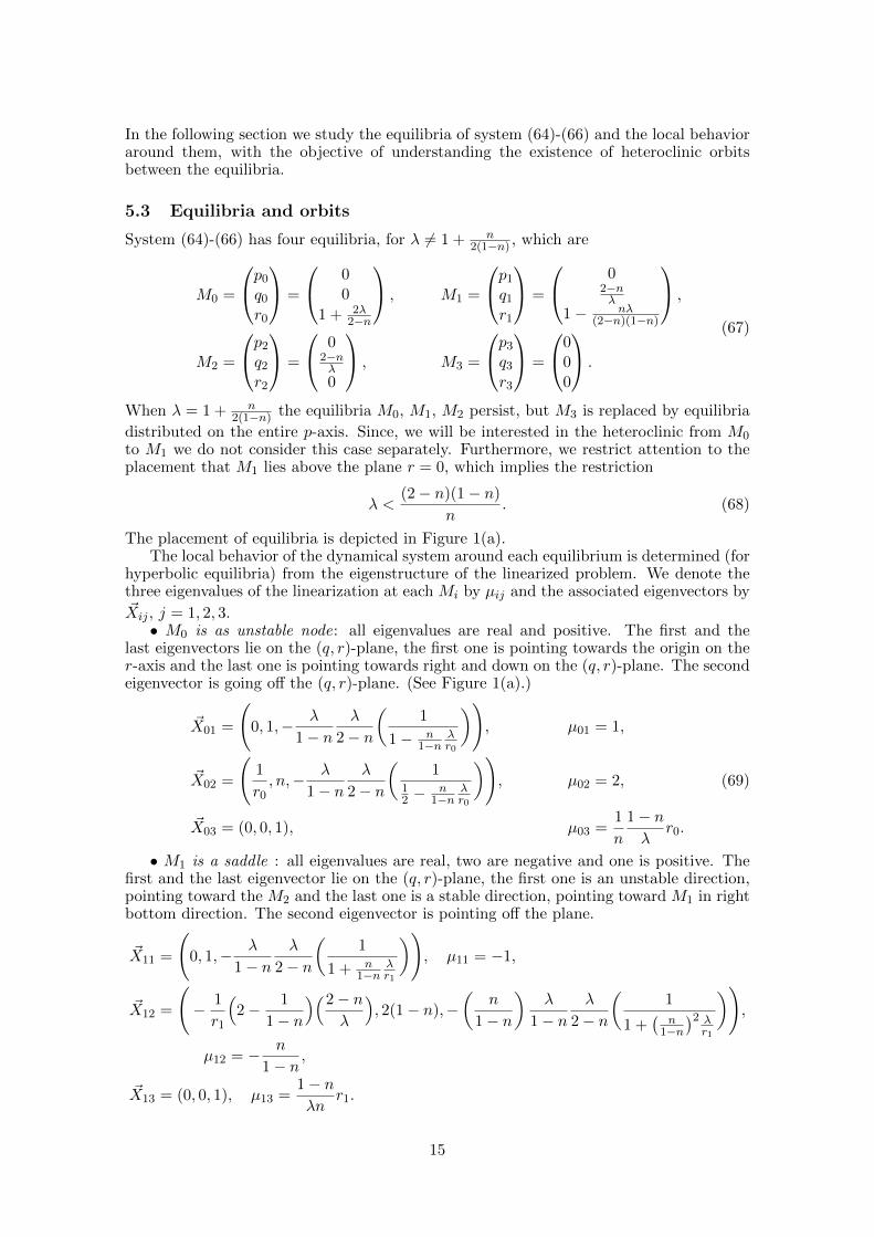
In the following section we study the equilibria of system (64)-(66) and the local behavioraround them, with the objective of understanding the existence of heteroclinic orbitsbetween the equilibria.

5.3 Equilibria and orbits

System (64)-(66) has four equilibria, for λ 6= 1 + n2(1−n) , which are

M0 =

p0

q0

r0

=

00

1 + 2λ2−n

, M1 =

p1

q1

r1

=

02−nλ

1− nλ(2−n)(1−n)

,

M2 =

p2

q2

r2

=

02−nλ0

, M3 =

p3

q3

r3

=

000

.

(67)

When λ = 1 + n2(1−n) the equilibria M0, M1, M2 persist, but M3 is replaced by equilibria

distributed on the entire p-axis. Since, we will be interested in the heteroclinic from M0

to M1 we do not consider this case separately. Furthermore, we restrict attention to theplacement that M1 lies above the plane r = 0, which implies the restriction

λ <(2− n)(1− n)

n. (68)

The placement of equilibria is depicted in Figure 1(a).The local behavior of the dynamical system around each equilibrium is determined (for

hyperbolic equilibria) from the eigenstructure of the linearized problem. We denote thethree eigenvalues of the linearization at each Mi by µij and the associated eigenvectors by~Xij , j = 1, 2, 3.• M0 is as unstable node: all eigenvalues are real and positive. The first and the

last eigenvectors lie on the (q, r)-plane, the first one is pointing towards the origin on ther-axis and the last one is pointing towards right and down on the (q, r)-plane. The secondeigenvector is going off the (q, r)-plane. (See Figure 1(a).)

~X01 =

(0, 1,− λ

1− nλ

2− n

(1

1− n1−n

λr0

)), µ01 = 1,

~X02 =

(1

r0, n,− λ

1− nλ

2− n

(1

12 −

n1−n

λr0

)), µ02 = 2, (69)

~X03 = (0, 0, 1), µ03 =1

n

1− nλ

r0.

• M1 is a saddle : all eigenvalues are real, two are negative and one is positive. Thefirst and the last eigenvector lie on the (q, r)-plane, the first one is an unstable direction,pointing toward the M2 and the last one is a stable direction, pointing toward M1 in rightbottom direction. The second eigenvector is pointing off the plane.

~X11 =

(0, 1,− λ

1− nλ

2− n

(1

1 + n1−n

λr1

)), µ11 = −1,

~X12 =

(− 1

r1

(2− 1

1− n

)(2− nλ

), 2(1− n),−

(n

1− n

)λ

1− nλ

2− n

(1

1 +(

n1−n)2 λr1

)),

µ12 = − n

1− n,

~X13 = (0, 0, 1), µ13 =1− nλn

r1.

15

(a) Equilibria of (p, q, r)-system and linearized vec-tor fields around

(b) Schematically illustrated target orbit betweenM0 and M1

Figure 1: Phase diagram. Features attributed to generic parameters are (i) M1 lies abovethe plane r = 0; (ii) µ31 > 0.

• M2 is a stable node: all eigenvalues are real and negative. The eigenvectors are thecoordinate basis vectors,

~X21 = (1, 0, 0), µ21 = − 1

λ

(1 +

n

2− nλ

),

~X22 = (0, 1, 0), µ22 = −1,

~X23 = (0, 0, 1), µ23 = − 1

n

1− nλ

r1.

• M3 is at the origin and is a saddle: all eigenvalues are real, the second eigenvalueis positive and the last eigenvalue is negative. The sign of the first eigenvalue bifurcatesby λ = 1 + n

2(1−n) ; it is negative if λ < 1 + n2(1−n) and is positive if λ > 1 + n

2(1−n) . The

eigenvectors are the coordinate basis vectors,

~X31 = (1, 0, 0), µ31 = − 1

λ

(1− 2(1− n)

2− nλ

),

~X32 = (0, 1, 0), µ32 = 1,

~X33 = (0, 0, 1), µ33 = − 1

n

1− nλ

r0.

5.4 Characterization of the heteroclinic orbit

In this section, we study the heteroclinic connections between the equilibrium points.Since there are four equilibria, the unstable and stable manifolds of the equilibria mightintersect in various ways and could conceivably produce multiple connections. We aim toidentify the one that is physically relevant and to construct it in phase space. We assertthat the relevant orbit joins M0 to M1 as η runs from −∞ to ∞. A schematic sketch ofthis orbit is depicted in Figure 1(b). Let us explain how that is singled out.

5.4.1 The behavior as η →∞

We will be interested in the orbit converging to the equilibrium M1. The reason is thefollowing: From the perspective of shear band formation, the strain of a localizing solution

16

should grow with time, as the material is loading. Note that if γ(x, t) grows polynomially

as tρ, then the ratio (t+γ0)γtγ ∼ ρ as t increases. On the other hand, the transformations

we imposed imply

r =u

γ=ξ

22−n U(ξ)

ξ2

2−n Γ(ξ)=U(ξ)

Γ(ξ)=U(x, τ)

Γ(x, τ)=

(t+ γ0)u(x, t)

γ(x, t)=

(t+ γ0)γtγ

.

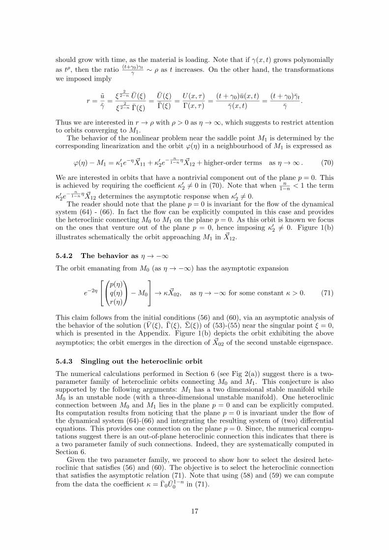
Thus we are interested in r → ρ with ρ > 0 as η →∞, which suggests to restrict attentionto orbits converging to M1.

The behavior of the nonlinear problem near the saddle point M1 is determined by thecorresponding linearization and the orbit ϕ(η) in a neighbourhood of M1 is expressed as

ϕ(η)−M1 = κ′1e−η ~X11 + κ′2e

− n1−nη ~X12 + higher-order terms as η →∞ . (70)

We are interested in orbits that have a nontrivial component out of the plane p = 0. Thisis achieved by requiring the coefficient κ′2 6= 0 in (70). Note that when n

1−n < 1 the term

κ′2e− n

1−nη ~X12 determines the asymptotic response when κ′2 6= 0.The reader should note that the plane p = 0 is invariant for the flow of the dynamical

system (64) - (66). In fact the flow can be explicitly computed in this case and providesthe heteroclinic connecting M0 to M1 on the plane p = 0. As this orbit is known we focuson the ones that venture out of the plane p = 0, hence imposing κ′2 6= 0. Figure 1(b)

illustrates schematically the orbit approaching M1 in ~X12.

5.4.2 The behavior as η → −∞

The orbit emanating from M0 (as η → −∞) has the asymptotic expansion

e−2η

p(η)q(η)r(η)

−M0

→ κ ~X02, as η → −∞ for some constant κ > 0. (71)

This claim follows from the initial conditions (56) and (60), via an asymptotic analysis ofthe behavior of the solution (V (ξ), Γ(ξ), Σ(ξ)) of (53)-(55) near the singular point ξ = 0,which is presented in the Appendix. Figure 1(b) depicts the orbit exhibiting the above

asymptotics; the orbit emerges in the direction of ~X02 of the second unstable eigenspace.

5.4.3 Singling out the heteroclinic orbit

The numerical calculations performed in Section 6 (see Fig 2(a)) suggest there is a two-parameter family of heteroclinic orbits connecting M0 and M1. This conjecture is alsosupported by the following arguments: M1 has a two dimensional stable manifold whileM0 is an unstable node (with a three-dimensional unstable manifold). One heteroclinicconnection between M0 and M1 lies in the plane p = 0 and can be explicitly computed.Its computation results from noticing that the plane p = 0 is invariant under the flow ofthe dynamical system (64)-(66) and integrating the resulting system of (two) differentialequations. This provides one connection on the plane p = 0. Since, the numerical compu-tations suggest there is an out-of-plane heteroclinic connection this indicates that there isa two parameter family of such connections. Indeed, they are systematically computed inSection 6.

Given the two parameter family, we proceed to show how to select the desired hete-roclinic that satisfies (56) and (60). The objective is to select the heteroclinic connectionthat satisfies the asymptotic relation (71). Note that using (58) and (59) we can computefrom the data the coefficient κ = Γ0U

1−n0 in (71).

17

The general heteroclinic orbit ϕ(η) satisfies, in a sufficiently small neighbourhood ofM0, the expansion

ϕ(η)−M0 = κ1eη ~X01 + κ2e

2η ~X02 + κ3e1n

1−nλr0η ~X03 + higher-order terms, (72)

as η → −∞. For n small, 1 < 2 < 1n

1−nλ r0, the first term in the right hand side of

(72) dominates the remaining terms. Therefore, (71) dictates that the coefficient κ1 = 0and thus (71) fixes one curve and reduces by one the degrees of freedom. Let us denoteby Φ(η) := (P (η), Q(η), R(η)) a heteroclinic orbit that emanates in the direction of the

eigenvector ~X02. There is one degree of freedom at our disposal provided by the translationinvariance of the selected orbit.

Having selected the curve Φ(η), we proceed to select the translation factor η0 as follows:Let κ2 be the constant associated to the asymptotic behavior of Φ(η) in (72). We set ourtarget heteroclinic

ϕ?(η) =

p(η)q(η)r(η)

=

P (η + η0)Q(η + η0)R(η + η0)

,

and compute

e−2η

p(η)q(η)r(η)

−M0

= e−2η

P (η + η0)Q(η + η0)R(η + η0)

−M0

→ κ2e2η0 ~X02, as η → −∞.

Therefore, given κ in (71), we compute η0 by

η0 =1

2log(κ2

κ

). (73)

In summary, there exists a two parameter family of heteroclinic orbits joining M0 and M1,whose existence is supported by the numerical calculations, and (71) singles out one orbitamong them.

5.5 A three-parameter family of focusing self-similar solutions

Among the parameters n, λ and the data Γ0, U0 and Σ0, only three are independent due to(58) and (59). Given n and two parameters, say Γ0 = Γ(0) and U0 = U(0) with Γ0 < U0,we select λ > 0 and the translaton factor η0 by (79):

λ =2− n

2

(U0

Γ0− 1

), κ = Γ0U

1−n0 . (74)

The inequality (68) restricts the data

1 <U0

Γ0<

2− nn

. (75)

Now, we pick one heteroclinic ϕ?(η) =(p(η), q(η), r(η)

)Thaving the desired asymptotic

behavior by the procedure described in Section 5.4.3. The solution is reconstructed byinverting (63) to obtain v, γ, u and σ,

v =1

n

(p−(1−n)q2−nrn

) 12−n

, γ =(prn) 1

2−n, σ =

(p−(1−n)rn

) 12−n

, u =(pr2) 1

2−n.

(76)

18

It is instructive to relate (p, q, r) to the original variables(v(x, t), γ(x, t), σ(x, t), u(x, t)

).

Using (62) we recover(V (ξ), Γ(ξ), U(ξ), Σ(ξ)

)which are smooth functions of ξ. More-

over, using (52) and (26), the original variables v, γ, σ and u = vx are reconstructed bythe formulas

v(x, t) =(

1 +t

γ0

) λn2−n

V

(x(

1 +t

γ0

)λ),

γ(x, t) = γ0

(1 +

t

γ0

)1+ 2λ2−n

Γ

(x(

1 +t

γ0

)λ),

σ(x, t) =1

γ0

(1 +

t

γ0

)−1−λ(1− n2−n )

Σ

(x(

1 +t

γ0

)λ),

u(x, t) =(

1 +t

γ0

) 2λ2−n

U

(x(

1 +t

γ0

)λ).

(77)

The focusing behavior of the profiles is readily deduced from the above formulas and isalso illustrated in the Figures 4(a)-4(d), obtained from the computed heteroclinic orbit.The asymptotic behavior of the profiles

(V , Γ, Σ, U

)as ξ → 0 and ξ → ∞ captures the

behavior of the localizing solution and is listed in the following proposition:

Proposition 5.1. For the orbit ϕ?(η), the corresponding profile(V , Γ, Σ, U

)defined in

[0,∞) by (62) satisfies the properties:

(i) At ξ = 0 it satisfies the boundary conditions

V (0) = Γξ(0) = Σξ(0) = Uξ(0) = 0, Γ(0) = Γ0, U(0) = U0.

(ii) The asymptotic behavior as ξ → 0 is given by

V (ξ) = U0ξ +O(ξ3), Γ(ξ) = Γ0 +O(ξ2),

Σ(ξ) =Un0Γ0

+O(ξ2), U(ξ) = U0 +O(ξ2).

(iii) The asymptotic behavior as ξ →∞ is given by

V (ξ) = O(1), Γ(ξ) = O(ξ−1

1−n ),

Σ(ξ) = O(ξ), U(ξ) = O(ξ−1

1−n ).

Indeed the behavior in (i) and (ii) follows readily from the analysis in Section (5.4)and the Appendix. To prove (iii): Note that the heteroclinic orbit ϕ?(η) must lie in theintersection W u(M0) ∩W s(M1) and thus satisfies as η → ∞ the asymptotic expansion

(70). The term multiplying e−η decays much faster than the term e−n

1−nη and can beignored. Using (70), together with (67), (69), we compute the asymptotic behavior

p(η) ∼ e−n

1−nη , q(η)→ 2− nλ

, r(η)→ 1− nλ

(2− n)(1− n)as η →∞ .

In turn, via (76),

γ(η) ∼ e−n

(1−n)(2−n)η , u(η) ∼ e−n

(1−n)(2−n)η . σ(η) ∼ en

2−nη as η →∞

and (iii) follows from (62) and ξ = eη.

19

Having identified the asymptotic behavior of(Γ, Σ, U

)associated to the selected hete-

roclinic orbit, we can identify the behavior of(γ, σ, u

). Using (77) and Proposition 5.1(iii),

we obtain:

(a) For the strain:

γ(0, t) = Γ0

(1 + t

γ0

)1+ 22−nλ

γ(x, t) ∼(

1 + tγ0

)1− n(2−n)(1−n)λ |x|−

11−n as t→∞ for x 6= 0.

The tip of the strain γ(0, t) grows at superlinear order and γ(x, t), x 6= 0, grows in sublinearorder as t → ∞. Recalling that the growth of the uniform shear motion is linear, thisobservation points to localization.

(b) For the strain rate

u(0, t) = U0

(1 + t

γ0

) 22−nλ

u(x, t) ∼(

1 + tγ0

)− n(2−n)(1−n)λ |x|−

11−n as t→∞ for x 6= 0.

u(x, t) decays to 0 for x 6= 0 in the presence of n > 0 as t→∞.

(c) For the stress

σ(0, t) =Un0Γ0

1

γ0

(1 + t

γ0

)−1−2λ 1−n2−n

,

σ(x, t) ∼(

1 + tγ0

)−1+ n2−nλ |x| as t→∞ for x 6= 0.

As time proceeds, the stress collapses at the origin quicker to 0 than at points x 6= 0.

6 Numerical Results

In this section we construct numerically the heteroclinic orbit proposed in Section 5.4 andschematically presented in Figure 1(b). To this end we numerically compute solutions ofthe dynamical system (64)-(66) using appropriate routines from the odesuite of MATLAB.Care has to be exercised to deal with the known difficulties in numerically computingheteroclinic orbits.

The first task is to compute the collection of heteroclinic orbits joining M0 and M1.Such heteroclinics appear as intersections of W u(M0), the unstable manifold of the equi-librium M0, and W s(M1), the stable manifold of the equilibrium M1. We capture thisintersection numerically by using a shooting argument. We start with initial conditionsnear M1 at the directions spanned by the stable eigenvectors of the equilibrium M1. Suchdata lie in the stable manifold W s(M1); we compute numerically the solution of (64)-(66) solving backwards in η. The orbits that tend near the equilibrium M0 are retainedand form a two dimensional manifold of heteroclinics, which comprises the intersectionW u(M0) ∩W s(M1). The result of the computation is depicted in Fig. 2(a).

It is expected from the asymptotic behavior in formula (72) that the heteroclinics

in this manifold will be separated to those approaching M0 along the eigenvector ~X01

(the blue curves) and one single orbit approaching in the direction ~X02. To capturecomputationally the latter, we proceed as follows. Starting now near M0 we compute the

solutions of (64)-(66) with initial data close to M0 in the tangent space spanned by ~X02

and ~X03. We note that the unstable manifold W u(M0) is the whole space and splits intothe blue curves (forming the heteroclinic surface) and the orange curves in the transversal

20

(a) Numerical plot of the surface formed byheteroclinic orbits (blue curves) comprisingW s(M1) ∩Wu(M0).

(b) A zoom around M0 depicting the inter-section of the surface of heteroclinics (bluecurves) with the part of the unstable man-ifold Wu(M0) associated to the directions~X02 and ~X03 (orange curves).

Figure 2: Numerical plot of the heteroclinic orbit (red dotted line).

directions. This second computation captures the orange curves. When the orbits reversedirectionality the computation captures the (red) heteroclinic emanating in the direction~X02; see Figure 2(b) for a zoom of this computation.

Having computed the heteroclinic orbit (p, q, r) of the dynamical system (64)-(66), ournext task is to introduce the computed solution to the transformation (77) to produce thenumerically computed form of the associated self-similar solution. The computed solutionis presented in Figures 4(a)-4(d). The graph is presented in terms of the original variablesv(x, t), γ(x, t), u(x, t) and σ(x, t) depicting the solution at various instances of time. FromFigures 4(a) - 4(d), one sees that initially all the variables are small perturbations of thecorresponding uniform shear solutions (15). These nonuniformities then are amplified andeventually develop a shear band. The strain and strain rate exhibit sharp peaks localizedaround the origin and the velocity field becomes a step like function, with the transitionagain occurring around the origin. The stress field initially assumes finite values, but asthe shear band forms it collapses to computable zero at the center of the band.

7 Discussions and Conclusions

We have considered a model for shear deformation of a viscoplastic material, with a yieldrelation depending the plastic strain γ and the strain rate γt, modeling a viscoplasticmaterial exhibiting strain softening and strain rate sensitivity, in the form of inverse andpower law respectively. The effects of those two mechanisms were first assessed at thelinearized level. The uniform shearing solutions are stable for n > 1, see [19], and weconsidered the range 0 < n < 1. In this parameter range, strain rate sensitivity alters thenature of instability from Hadamard instability to Turing instability.

Then we turned into explaining the emergence of a coherent structure in the nonlinearregime. An effective equation is derived which captures the combined effect of the compe-tition between strain-rate hardening and strain-softening. We analyzed a class of focusingself-similar solutions exploiting the invariance properties of the underlying model. Thisoffers a quantitative way for describing the development of singularity beyond the lin-earized level. The associated localized solution arises as a heteroclinic orbit of an inducedautonomous dynamical system. For a certain range of the parameters, the existence ofsuch a heteroclinic orbit was shown numerically. The associated profiles exhibit coherentlocalizing structures that have the morphology of shear bands. The result hinges on acomputational construction of the heteroclinic orbit. The proof of existence of the het-

21

(a) Detected orbit (b) Zoom-in of orbit near M0

Figure 3: Simulation of the heteroclinic orbit (n = 0.3 and λ = 2).

eroclinic orbit requires advanced results from dynamical systems, the geometric singularperturbation theory, and is presented in [15].

Appendix : Proof of (71)

To establish the claim (71), the starting point is the boundary conditions (56) and (60).We compute a Taylor expansion of the variables p(log ξ), q(log ξ) and r(log ξ) near ξ = 0.Initial conditions (60) imply an asymptotic behavior near ξ = 0 of the form

V (ξ) = U(0)ξ + o(ξ2),

Γ(ξ) = Γ(0) +ξ2

2Γξξ(0) + o(ξ2),

Σ(ξ) = Σ(0) +ξ2

2Σξξ(0) + o(ξ2),

U(ξ) = U(0) +ξ2

2Uξξ(0) + o(ξ2).

The values of the variables and their derivatives evaluated at ξ = 0 can be inferred bydifferentiating system (53)-(55) repeatedly. After a straightforward calculation, we find

V (0) = 0, Vξ(0) = U(0) = Γ(0)(

1 +2λ

2− n

),

Σ(0) =U(0)n

Γ(0), Γξ(0) = Σξ(0) = Uξ(0) = 0,

and

Γξξ(0) = −(Γ(0)2U(0)1−n) λ

2− nλ

1− n

(1

12 −

n1−n

λr0

)1

λ,

Uξξ(0) = −(Γ(0)2U(0)1−n) λ

2− nλ

1− n

(r0 + 2λ

12 −

n1−n

λr0

)1

λ.

22

−3 −2 −1 0 1 2 3x

10-2

10-1

100γ(x

,t)

t=0

t=0.1

t=0.2

t=0.3

t=0.4

t=0.5

(a) strain (γ)

−3 −2 −1 0 1 2 3x

10-1

100

101

u(x

,t)

t=0t=0.1t=0.2t=0.3t=0.5

(b) strain rate (u)

−20 −10 0 10 20x

−4

−3

−2

−1

0

1

2

3

4

v(x,t)

t=0t=0.1t=0.2t=0.3t=0.5

(c) velocity (v)

−20 −10 0 10 20x

100

101

102

σ(x

,t)

t=0t=0.1

t=0.2t=0.3

t=0.5

(d) stress (σ)

Figure 4: The localizing solution, for n = 0.05 and λ = 10, sketched in the originalvariables v, γ, u, σ. All graphs except v are in logarithmic scale.

Then, the Taylor expansion of p(log ξ) near ξ = 0 gives

p(log ξ) =γ

σ=ξ

22−n Γ

ξ2

2−n Σ= ξ2 Γ

Σ= ξ2 Γ(0)

Σ(0)+ o(ξ2) = Γ(0)2U(0)−nξ2 + o(ξ2) ,

and the Taylor expansion of q(log ξ) is

q(log ξ) = nv

σ= n

ξn

2−n V

ξ−1+ n2−n Σ

= nξV

Σ= n

[ξV (0)

Σ(0)+ ξ2 V (0)

Σ(0)

(Vξ(0)

V (0)−

Σξ(0)

Σ(0)

)+ o(ξ2)

]= nΓ(0)U(0)1−nξ2 + o(ξ2).

Finally, notice first that

r(log ξ) =u

γ=ξ

22−n U

ξ2

2−n Γ=U

Γand thus lim

ξ→0r(log ξ) =

U(0)

Γ(0)= 1 +

2λ

2− n= r0. (78)

The Taylor expansion of r(log ξ)− r0 near ξ = 0 yields

r(log ξ)− r0 =U

Γ− U(0)

Γ(0)= ξ

U(0)

Γ(0)

(Uξ(0)

U(0)−

Γξ(0)

Γ(0)

)+

1

2ξ2

[Uξξ(0)

Γ(0)− 2

Uξ(0)Γξ(0)

Γ2(0)+ U(0)

(−

Γξξ(0)

Γ2(0)+ 2

(Γξ(0)

)2Γ3(0)

)]+ o(ξ2)

= −(Γ(0)U(0)1−n) λ

2− nλ

1− n

(1

12 −

n1−n

λr0

)ξ2 + o(ξ2) .

23

From log ξ = η, we conclude that

e−2η

p(η)q(η)r(η)

−M0

→ Γ(0)U(0)1−n ~X02, as η → −∞.

Now (56) specifies Γ(0) and in view of (78),

κ = Γ0U1−n0 , where U0 = Γ0

(1 +

2λ

2− n

). (79)

Notice that Γ0 has the role of determining a translation factor of the curve.

Remark 7.1. Let(Γ, V , Σ

)be a solution of (53)-(55) with (56),(60) and ϕ?(η) be the

corresponding heteroclinic orbit of (64)-(66). Further, let(ΓA, VA, ΣA

)be the rescaled

solution as in (61) and ϕ?A(η) be the corresponding heteroclinic orbit. Then ϕ?A(η) =ϕ?(η + η0) with η0 = logA.

Let η0 = logA. Then

vA(

log ξ)

:= ξn

2−n VA(ξ) = (Aξ)n

2−n V (Aξ) = v(η + η0

),

γA(

log ξ)

:= ξ2

2−n ΓA(ξ) = (Aξ)2

2−n Γ(Aξ) = γ(η + η0

),

σA(

log ξ)

:= ξ−1+ n2−n ΣA(ξ) = (Aξ)−1+ n

2−n Σ(Aξ) = σ(η + η0

)and hence ϕ?A(η) = ϕ?(η + η0).

Acknowledgements

Research supported by King Abdullah University of Science and Technology (KAUST).

References

[1] L. Anand, K.H. Kim and T.G. Shawki, Onset of shear localization in viscoplasticsolids, J. Mech. Phys. Solids 35 (1987), 407–429.

[2] Th. Baxevanis and N. Charalambakis, The role of material non-homogeneitieson the formation and evolution of strain non-uniformities in thermoviscoplastic shear-ing, Quart. Appl. Math. 62 (2004), 97–116.

[3] Th. Baxevanis, Th Katsaounis, and A. E. Tzavaras, Adaptive finite elementcomputations of shear band formation, Math. Models Methods Appl. Sci. 20 (2010),423–448.

[4] M. Bertsch, L. Peletier, and S. Verduyn Lunel, The effect of temperaturedependent viscosity on shear flow of incompressible fluids, SIAM J. Math. Anal. 22(1991), 328–343.

[5] T.J. Burns and M.A. Davies, On repeated adiabatic shear band formation duringhigh speed machining, International Journal of Plasticity 18 (2002), 507–530.

[6] L. Chen and R.C. Batra , The asymptotic structure of a shear band in mode-IIdeformations. International Journal of Engineering Science 37 (1999), 895–919.

[7] R.J. Clifton, High strain rate behaviour of metals, Applied Mechanics Review 43(1990), S9–S22.

24

[8] R. J. Clifton, J. Duffy, K. A. Hartley, and T. G. Shawki, On criticalconditions for shear band formation at high strain rates. Scripta Metallurgica 18(1984), 443–448.

[9] C. M. Dafermos and L. Hsiao, Adiabatic shearing of incompressible fluids withtemperature-dependent viscosity. Quart. Applied Math. 41 (1983), 45–58.

[10] Donald J Estep, Sjoerd M Verduyn Lunel, and Roy D Williams, Analysisof Shear Layers in a Fluid with Temperature-Dependent Viscosity, J. Comp. Physics173 (2001), 17–60.

[11] C. Fressengeas and A. Molinari, Instability and localization of plastic flow inshear at high strain rates, J. Mech. Physics of Solids 35 (1987), 185–211.

[12] J.W. Hutchinson and K.W. Neale, Influence of strain-rate sensitivity on neckingunder uniaxial tension, Acta Metallurgica 25 (1977), 839–846.

[13] Th. Katsaounis and A.E. Tzavaras, Effective equations for localization and shearband formation, SIAM J. Appl. Math. 69 (2009), 1618–1643.

[14] Th. Katsaounis, J. Olivier, and A.E. Tzavaras, Emergence of coherent local-ized structures in shear deformations of temperature dependent fluids, arXiv preprintarXiv:1411.6131, (2014).

[15] M.-G. Lee and A.E. Tzavaras, Existence of localizing solutions in plasticity viathe geometric singular perturbation theory. (preprint) 2016.

[16] A. Molinari and R.J. Clifton, Analytical characterization of shear localizationin thermoviscoplastic materials, Journal of Applied Mechanics 54 (1987), 806–812.

[17] T. G. Shawki and R. J. Clifton, Shear band formation in thermal viscoplasticmaterials, Mechanics of Materials 8 (1989), 13–43.

[18] A.M. Turing, The chemical basis of morphogenesis. Phil. Trans. R. Soc. London B,237 (1952), 37–72.

[19] A.E. Tzavaras, Plastic shearing of materials exhibiting strain hardening or strainsoftening, Archive for Rational Mechanics and Analysis 94 (1986), 39–58.

[20] A.E. Tzavaras, Effect of thermal softening in shearing of strain-rate dependentmaterials. Archive for Rational Mechanics and Analysis, 99 (1987), 349–374.

[21] A.E. Tzavaras, Strain softening in viscoelasticity of the rate type. J. Integral Equa-tions Appl. 3 (1991), 195–238.

[22] A.E. Tzavaras, Nonlinear analysis techniques for shear band formation at highstrain-rates, Applied Mechanics Reviews 45 (1992), S82–S94.

[23] J.W. Walter, Numerical experiments on adiabatic shear band formation in onedimension. International Journal of Plasticity 8 (1992), 657–693.

[24] T.W. Wright, The Physics and Mathematics of Shear Bands. Cambridge Univ.Press, 2002.

[25] T.W. Wright and J.W. Walter, On stress collapse in adiabatic shear bands, J.Mech. Phys. of Solids 35 (1987), 701–720.

[26] F.H. Wu and L.B. Freund, Deformation trapping due to thermoplastic instabilityin one-dimensional wave propagation, J. Mech. Phys. of Solids 32 (1984), 119–132.

[27] C. Zener and J. H. Hollomon, Effect of strain rate upon plastic flow of steel,Journal of Applied Physics 15 (1944), 22–32.

25