lectures on applied reactor technology and nuclear … th intro... · applied reactor technology...

Applied Reactor Technology and Nuclear Power Safety Chapter 6

Lectures on Applied Reactor Technology and Nuclear Power Safety

Part II – Nuclear Reactor Thermal-Hydraulics

Henryk Anglart Nuclear Reactor Technology Division

Department of Energy Technology KTH

Spring 2005

________________________________________________________________________ Henryk Anglart Rev. 0 Page 6-1


CONTENTS OF PART II Chapter 6. Introduction to Thermal-Hydraulic Analysis of Nuclear Reactor Cores 6.1 Thermal Issues in Nuclear Reactor Cores 6.2 Power Generation in Nuclear Reactor Cores 6.3 Principles of Fluid Flow and Heat Transfer Chapter 7. Thermal-Hydraulic Analysis of Single-Phase Flows in Heated Channels 7.1 Clad-Coolant Heat Transfer in Channels with Single-Phase Flow 7.2 Coolant Enthalpy Distribution in Heated Channels 7.3 Temperature Distribution in Fuel Elements 7.4 Pressure Distribution in Channels with Single-Phase Flow Chapter 8. Thermal-Hydraulic Analysis of Two-Phase Flows in Heated Channels 8.1 Onset of Nucleate Boiling 8.2 Subcooled and Saturated Flow Boiling 8.3 Occurrence of Critical Heat Flux 8.4 Post-CHF Heat Transfer 8.5 Void Fraction Distribution in Boiling Channels 8.6 Pressure Distribution in Boiling Channels Chapter 9. Thermal-Hydraulic Design of Nuclear Reactor Cores 9.1 Basis of Thermal-Hydraulic Core Analysis 9.2 Hot Channel Factors 9.3 Heat Flux Limitations 9.4 Computer Codes in Nuclear Reactor Thermal-Hydraulics Chapter 10. Dynamics and Stability of Nuclear Reactor Cores 10.1 Nuclear Reactor Core Dynamics 10.2 Nuclear Reactor Core Stability



6. Introduction to Thermal-Hydraulic Analysis of Nuclear Reactor Cores

The energy released in nuclear fission is transformed through the kinetic energy of fission reaction products into heat generated in the reactor fuel elements. This heat must be removed from the reactor core and used to generate electrical power. The sequence of energy transformations in a typical Boiling Water Reactor (BWR) nuclear power plant is termed in present lectures as thermal energy cycles. The cycles can be put into two main categories: (a) in-vessel thermal energy cycles and (b) ex-vessel thermal energy cycles. A general view of a nuclear power plant is shown in Fig. 6.0.1.

Figure 6.0.1. General view of a nuclear power plant. All thermal processes that take place inside the nuclear reactor vessel belong to the category of in-vessel thermal energy cycles. Figure 6.0.2 shows the main stages of the in-vessel thermal energy cycles in case of a BWR nuclear power plant.



Fission-product

energy in fuel Conduction through fuel

Transfer across fuel-clad gas gap

Conduction across clad

Transfer from clad surface to coolant

Forced convection in coolant in fuel assemblies

Steam generation due to boiling

Steam separation

Figure 6.0.2. In-vessel thermal energy cycles in a BWR nuclear power plant. Figure 6.0.3 shows a schematic of ex-vessel thermal energy cycles in a typical Boiling Water Reactor (BWR) nuclear power plant. Corresponding schematic for Pressurized Water Reactor (PWR) nuclear power plant is shown in Fig. 6.0.4.

Figure 6.0.3. Schematic of ex-vessel thermal energy cycles in BWR nuclear power plants.



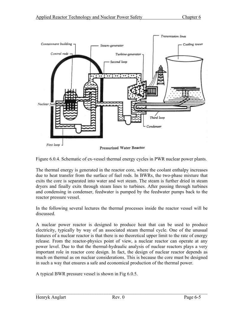
Figure 6.0.4. Schematic of ex-vessel thermal energy cycles in PWR nuclear power plants. The thermal energy is generated in the reactor core, where the coolant enthalpy increases due to heat transfer from the surface of fuel rods. In BWRs, the two-phase mixture that exits the core is separated into water and wet steam. The steam is further dried in steam dryers and finally exits through steam lines to turbines. After passing through turbines and condensing in condenser, feedwater is pumped by the feedwater pumps back to the reactor pressure vessel. In the following several lectures the thermal processes inside the reactor vessel will be discussed. A nuclear power reactor is designed to produce heat that can be used to produce electricity, typically by way of an associated steam thermal cycle. One of the unusual features of a nuclear reactor is that there is no theoretical upper limit to the rate of energy release. From the reactor-physics point of view, a nuclear reactor can operate at any power level. Due to that the thermal-hydraulic analysis of nuclear reactors plays a very important role in reactor core design. In fact, the design of nuclear reactor depends as much on thermal as on nuclear considerations. This is because the core must be designed in such a way that ensures a safe and economical production of the thermal power. A typical BWR pressure vessel is shown in Fig 6.0.5.



Figure 6.0.5. BWR pressure vessel. Reactor pressure vessel contains internal structures, in which the most important one is the nuclear reactor core. The reactor core, in turn, consists of hundred of so-called fuel assemblies. Fuel assemblies contain cylindrical fuel rods organized in square or triangular

________________________________________________________________________ Henryk Anglart Rev. 0 -6


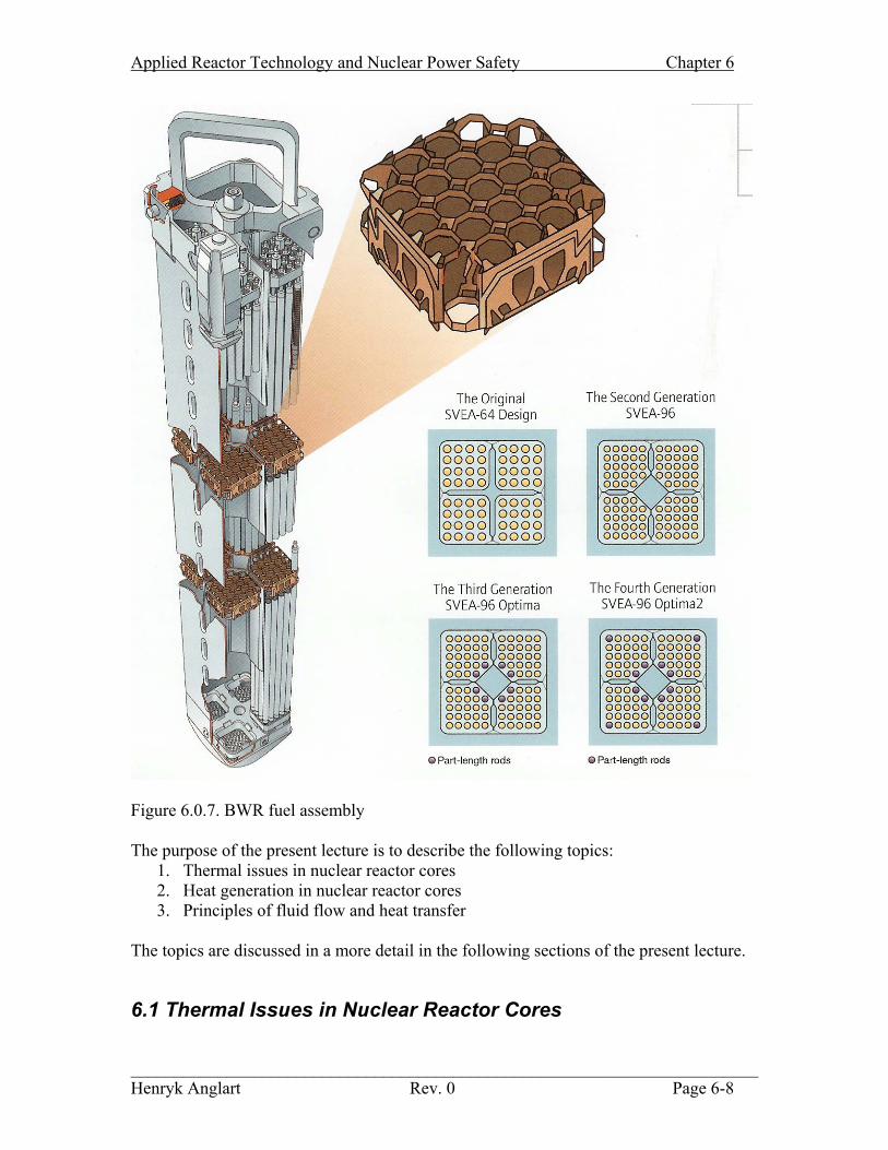
lattices. An example of a PWR fuel assembly is shown in Fig. 6.0.6 and an example of a BWR fuel assembly is shown in Fig. 6.0.7.

Figure 6.0.6. PWR fuel assembly.



Figure 6.0.7. BWR fuel assembly The purpose of the present lecture is to describe the following topics:

1. Thermal issues in nuclear reactor cores 2. Heat generation in nuclear reactor cores 3. Principles of fluid flow and heat transfer

The topics are discussed in a more detail in the following sections of the present lecture.

6.1 Thermal Issues in Nuclear Reactor Cores



There are several existing reactor concepts in which heat transfer solutions depend on particular design concepts and the choice of coolant. Although each reactor design has its own specific thermal problems, the solution of these problems can be approached in standard engineering manners that involve the fluid flow and heat transfer analysis. The effort to integrate the heat transfer and fluid mechanics principles to accomplish the desired rate of heat removal from the reactor fuel is termed as the thermal-hydraulic design of a nuclear reactor. An important difference between nuclear power plants and conventional power plants is that in the latter the temperature is limited to that resulting from combustion of coal, oil or gas, whereas it can increase continuously in a nuclear reactor in which the rate of heat removal is less than the rate of heat generation. Such situation could lead to the core damage. For a given reactor design, the maximum operating power is limited by some temperature in the system. There are several possible factors that will set the limit temperature (and thus the reactor power): material changes of some construction material in the reactor, allowable thermal stresses or influence of temperature on corrosion. Thus the maximum temperature in a nuclear reactor core must be definitely established under normal reactor operation and this is the goal of the thermal-hydraulic design and analysis of nuclear reactor cores. In nuclear reactors the construction materials must be chosen not only on the basis of the thermo-mechanical performance, but also (and often exclusively) on the basis of the nuclear properties. Beryllium metal, for example, is an excellent material for use as moderator and reflector, but it is relatively brittle. Austenitic stainless steels are used as the cladding for fast reactor fuels, but they tend to swell as a result of exposure at high temperatures to fast neutrons. Another peculiarity (and factor that adds problem) of nuclear reactors is that the power densities (e.g. power generated per unit volume) are very high. This is required by economical considerations. That leads to power densities of approximately 100 MWt/m3 in PWRs and 55 MWt/m3 in BWRs. A typical sodium-cooled commercial fast breeder reactor has a power density as high as 500 MWt/m3. In conventional power plants is of the order of 10 MWt/m3.

6.2 Power Generation in Nuclear Reactor Cores The energy released in nuclear fission reaction is distributed among a variety of reaction products characterized by different range and time delays. In thermal design, the energy deposition distributed over the coolant and structural materials is frequently reassigned to the fuel in order to simplify the thermal analysis of the core. The volumetric fission heat source in the core can be found as,

( ) ( ) ( )EEdENwq if

ii

if ,)(

0

)()( rrr φσ∫∑∞

=′′′ . (6.2.1)



Here is the recoverable energy released per fission event. Since the flux and the number density of the fuel vary across the reactor core, there will be a corresponding variation in the fission heat source.

)(ifw

The simplest model of fission heat distribution would correspond to a bare, homogeneous core. One should recall here the one-group flux distribution for such geometry given as,

( )

=

Hz

Rr

Jzr ~cos~, 00

πνφ . (6.2.2)

Here R~ and H~ are effective core dimensions that include extrapolation lengths as well as an adjustment to account for a reflected core. Having a fuel rod located at r = rf distance from the centerline of the core, the volumetric fission heat source becomes a function of the axial coordinate, z, only,

Σ=′′′

Hz

Rr

Jwzq fff ~cos~

405.2)( 00

πφ . (6.2.3)

There are numerous factors that perturb the power distribution of the reactor core, and the above equation will not be valid. For example fuel is usually not loaded with uniform enrichment. At the beginning of core life, higher enrichment fuel is loaded toward the edge of the core in order to flatten the power distribution. Other factors include the influence of the control rods and variation of the coolant density. All these power perturbations will cause a corresponding variation of temperature distribution in the core. A usual technique to take care of these variations is to estimate the local working conditions (power level, coolant flow, etc) which are the closest to the thermal limitations. Such part of the core is called hot channel and the working conditions are related with so-called hot channel factors. One common approach to define hot channel is to choose the channel where the core heat flux and the coolant enthalpy rise is a maximum. Working conditions in the hot channel are defined by several ratios of local conditions to core-averaged conditions. These ratios, termed the hot channel factors or power peaking factors will be considered in more detail in coming lectures. However, it can be mentioned already here that the basic initial plant thermal design relay on these factors.

6.3 Principles of Fluid Flow and Heat Transfer 6.3.1 Heat Conduction



Heat conduction refers to the transfer of heat by means of molecular interactions without any accompanying macroscopic displacement of matter. The flow of heat by conduction is governed by the Fourier law: ( ) ( tTt ,, rrq ∇−=′′ )λ (6.3.1)

where [W/m( t,rq ′′ ) 2] is the heat flux vector expressing the rate at which heat flows across a surface at location r and time t, T(r,t) [K] is the local temperature and λ [W m-1 K-1] is the thermal conductivity. A non-stationary temperature distribution in an arbitrary volume is described by the following equation, resulting from a simple energy balance for an arbitrary volume in the solid:

[ ] ( ) ( ttqtTtctt

,,),(),(),( rqrrrr ′′⋅∇−′′′=∂∂ ρ )

)

(6.3.2)

Here ( t,rρ [kg m-3] is the density of the solid material, c(r,t) [J kg-1 K-1] is the specific heat of the solid material and [W m( t,rq ′′ ) -3] is the heat source per unit volume. Substituting Eq. (6.3.1) into Eq. (6.3.2) yields the heat conduction equation:

[ ] ( tqtTtTtctt

,),(),(),(),( rrrrr ′′′=∇⋅∇−∂∂ λρ ). (6.3.3)

Distribution of temperature in any arbitrary volume can be found from Eq. (6.3.3) provided that the boundary and the initial conditions are known. The initial conditions are typically specified by a given temperature distribution in the whole region of interest at given time t = t0. Usually t0 = 0 and the initial condition can be written as, ( ) )(0, rr fT = , (6.3.4)

where f(r) is a given function of spatial coordinates. The boundary conditions can be specified in several different ways, depending on what kind of a parameter is known at the boundary. If the boundary temperature is known, the boundary conditions of the first kind (or the Dirichlet boundary conditions) are specified: ( ) ),(, ttT

Brrr

rϕ=

= (6.3.5)



Here rB are coordinates that describe the region boundaries where the temperature is a known function of time. If the boundary heat flux is known, the boundary conditions of the second kind (or the Neumann boundary conditions) are specified:

( ) ( ) ),(,, tn

tTtqB

Brrr

rrrr

φλ =∂

∂−≡

==

(6.3.6)

If a convective heat transfer to fluid with a known bulk temperature takes place, the boundary conditions of the third kind (or the Newton boundary conditions) are specified:

( ) ( ) ( )[ *,,,BB

B

tTtThn

tTf rrrr

rr

rrr==

=

−=∂

∂− λ ] (6.3.7)

where h [W m-2 K-1] is the convective heat transfer coefficient and ( ) *,

Btf rr

r=

T is the fluid

bulk temperature (notation r indicates that this value is not at the boundary location but at a certain distance from the boundary, equivalent to the thickness of the boundary layer).

*Br=

If two solid bodies are in contact with each other, the boundary conditions of the fourth kind are specified:

( ) ( ) ( ) ( )BB

BB ntT

ntTtTtT

rrrrrrrr

rrandrr==

== ∂∂

−=∂

∂−=

,,,, 22

1121 λλ (6.3.8)

Example 6.3.1. Steady-state heat conduction through an infinite cylindrical wall. Figure 6.3.1 shows the geometry and the boundary conditions of the case considered in the present example.

q’’

Tf

r1 r2 r

Figure 6.3.1 Steady-state heat conduction through an infinite cylindrical wall.



The conduction equation can be simplified to:

0=

drdTr

drd , (6.3.9)

and boundary conditions,

( frrrrrr

TThdrdTq

drdT

−=−′′=−=

==2

21

, λλ ) (6.3.10)

Solving Eq. (6.3.9) yields,

DrCT += ln (6.3.11) Substituting Eq. (6.3.11) into boundary conditions (6.3.10) yields the following system of two equations with two unknowns C and D:

( )

+

′′+=⇒

+−−=⇒−+=−

′′−=⇒′′=−

22

1

22

22

1

1 lnln,ln

,r

hrrqTD

TrChrCDTDrCh

rC

rqCqrC

f

ff

λλλλ

λλ

The solution is thus,

ff Thr

rqrrrqT

hrrqrrqrrqT +

′′+

′′=+

′′+

′′+

′′−=

2

121

2

12

11 lnlnlnλλλ

(6.3.12)

6.3.2 Laminar and Turbulent Flows The three basic laws of conservation of mass, momentum and energy are used to describe the fluid motion. The equations for incompressible flows are as follows,

( ) 0=vdiv (6.3.13)

pDtD

∇−⋅∇+= τgv ρρ (6.3.14)

( ) Φ+∇+= TdivDtDp

DtDH λρ (6.3.15)

New variables introduced in Eqs. (6.3.13) through (6.3.15) are as follows: v [m s-1] velocity vector, τ [N m-2] - the shear stress in the fluid and Φ [N s-1] - the viscous dissipation term.



When fluid flows in a straight pipe with low velocity the fluid particles move in straight lines parallel to the axis of the pipe. Such flow is called the laminar flow. The majority of fluids obey the Newton’s equation that relates the strains and stresses in the flow. The equation can be written in a general form as follows,

( )[ ]Tvvτ ∇+∇= µ (6.3.16) Here [N mτ -2] is the shear stress in the fluid, µ [Pa s] is the molecular dynamic viscosity of fluid and v [m s-1] is the fluid velocity vector. The expression in the rectangular parentheses is the so-called deformation tensor (or rather a double of it). For a laminar flow in a pipe, Eq. (6.3.16) becomes,

drdvzµτ = (6.3.17)

Assuming laminar, stationary, adiabatic flow of a Newtonian fluid in a vertical tube, Eqs. (6.3.13) through (6.3.17) yield:

vg 20 ∇++−∇= µρp (6.3.18) Assuming further that the pressure gradient is known, Eq. (6.3.18) can be solved for velocity as follows. In cylindrical coordinate system for present conditions the following is valid:

=∇

drdr

drd

r12 (6.3.19)

Also the velocity vector v reduces only to its axial component vz (other components are equal to zero due to the flow symmetry and the fully developed flow conditions). Thus:

=Π≡

−∇drdvr

drd

rgp z1

µρ (6.3.20)

Equation (6.3.20) can be solved as,

DrCrvrCr

drdvCr

drdvrr

drdvr

drd

zzzz ++

Π=⇒+

Π=⇒+

Π=⇒Π=

ln

422

22

The constants C and D are found from boundary conditions: vz is limited at r=0, therefore C = 0. For r = R (at the pipe wall), the velocity is equal to zero, that is vz = 0. Thus:



−

Π−=⇒

Π−=

222

144 R

rRvRD z (6.3.21)

Eq. (6.3.21) describes the so-called Poiseuille paraboloid, which represent the velocity distribution in a fully developed laminar flow in a tube. The average velocity in the tube is found as,

2

02 82)(1 Rrdrrv

RU

R

z µπ

πΠ−

=⋅≡ ∫ (6.3.22)

The wall shear stress can be calculated as,

RUR

drdvr

Rr

zRrw

µµττ 42

)( =Π

−=−≡−==

= (6.3.23)

Even though the wall shear stress is proportional to mean velocity (laminar flow), it is customary to nondimensionalize wall shear with the pipe dynamic pressure 22Uρ . There are two definitions commonly used in literature:

factorfrictionDarcyU

w =≡2

42ρτλ (6.3.24)

factorfrictionFanningU

C wf ==≡ λ

ρτ

41

22 (6.3.25)

Substituting Eq. (6.3.24) and (6.3.25) into (6.3.23) yields the classic relations,

Re16

Re64

== fCλ , (6.3.26)

where the Reynolds number appearing in Eq. (6.3.26) is defined as,

µρUD

=Re . (6.3.27)

Here D = 2 R is the pipe diameter. Laminar flow solutions shown above are in good agreement with experiments. Such flows undergo, however, transition to turbulent flows at approximately Re = 2000. For flows with Re = 3000 or higher the flow is fully turbulent and Eqs. (6.3.26) are not valid. For turbulent flows in pipes, H. Blasius obtained experimental data and proposed the following correlation for the Fanning friction factor:



25.0Re0791.0

=fC (6.3.28)

Commercial tubes have roughness (somewhat different from sand-grain behavior) and for such case C.F. Colebrook devised the following formula,

+−=

λλ Re51.2

7.3log0.21

10Dk . (6.3.29)

Here k is the pipe roughness. As can be seen, the Colebrook formula is implicit, that is one has to iterate to findλ . This annoyance can be avoided by instead using an explicit formula given by Haaland (1983),

+

−=

Re9.6

7.3log8.11 11.1

10Dk

λ (6.3.30)

Both formulas are in a very good agreement with each other. 6.3.3 Solid-Fluid Heat Transfer Heat transfer from the clad surface to the coolant is often described by the Newton’s law of cooling,

( )fw TThq −=′′ , (6.3.31) where q’’ [W m-2] is the heat flux at the clad surface, h [W m-2 K-1] is the convective heat transfer coefficient, Tw [K] is the clad surface temperature and Tf [K] is the fluid (coolant) bulk temperature. The convective heat transfer coefficient depends upon the fluid properties and flow conditions. Its determination is discussed below. Equation (6.3.31) is applicable for all kinds of flows: laminar and turbulent; for both gases and liquids, and describes a heat transfer mechanism which is termed the convection. When the fluid motion is caused by pumps, fans, or in general by pressure differences, the forced convection takes place. Otherwise when fluid motion is caused be density differences in the fluid, the natural convection occurs. The simplicity of Eq. (6.3.31) is deceiving, however. In fact, the heat transfer coefficient h is hiding the complexity of the solid-fluid heat transfer, and, as can be expected, a proper correlation must be used to obtain the coefficient which will be valid for specific flow conditions. In essentially all cases of reactor cooling where forced convection is used, the coolant is under turbulent flow conditions. Satisfactory predictions of heat transfer coefficients in long, straight channels of uniform cross section can be made on the assumption that the only variables involved are the mean velocity of the fluid coolant, the diameter (or equivalent diameter) of the coolant channel, the density, heat capacity, viscosity, and



thermal conductivity of the coolant. Using the dimensional analysis it can be shown that the heat transfer coefficient for turbulent flow conditions can be expressed in terms of three dimensionless numbers: the Reynolds number (Re), the Nusselt number (Nu) and the Prandtl number (Pr). Dittus-Boelter proposed the following correlation for long straight channels:

33.08.0 PrRe023.0Nu = , (6.3.32) where,

λhD

=Nu , (6.3.33)

λµpc

=Pr , (6.3.34)

and Reynolds number given by Eq. (6.3.27). All physical properties should be evaluated at the bulk temperature of fluid. Exercise 13. A cylindrical core has the extrapolated height and extrapolated radius equal to 3.8 m and 3.2 m, respectively. Calculate the volumetric heat source ratio between the point located in the middle of the central fuel assembly and the point located in a fuel assembly with a distance rf = 1.5 m from the core center and at z = 2.5 m from the inlet of the assembly. Exercise 14. A cylindrical wall with the internal diameter equal to 8 mm and thickness 0.5 mm is heated on the internal surface with a heat flux equal to 1 MW m-2. Calculate the temperature difference between the inner and the outer surface of the wall, assuming that the thermal conductivity of the wall material is equal to 16 W m-1 K-1. What will be the heat flux on the outer surface of the wall? Exercise 15. In a horizontal pipe with an internal diameter equal to 10 mm flows water at pressure p = 70 bar and at the saturation temperature. Calculate the wall shear stress change when mass flux of water increases from 50 to 2000 kg m-2 s-1. Assume that the water density and the dynamic viscosity are constant and equal to 740 kg m-3 and 1.0x10-

4 Pa s, respectively. Exercise 16. Heat transfer through cylindrical wall



r3 = 18

L = 1000

Q

TL

r1= 8

r2 = 10

r

Fig 6.3.2 Heat conduction through cylindrical wall Tasks For a uniform heat flux and given total heat source Q = 2.5 x 104 W, wall conductivity coefficient λ1 = 16 Wm-1K-1 and liquid temperature TL = 323 °C:

1. write shell balance for energy diffusion in the cylindrical solid, 2. state proper boundary conditions (boundary value problem), 3. calculate temperature distribution in the cylindrical solid, T ( )rf=

Obtain the heat transfer coefficient from the Dittus-Boelter correlation: , 6433.08.0 10Re103PrRe023.0 <<×=

hDgivenforNu Conductivity, heat capacity and dynamic viscosity of water are constant values: λ2 = 0.5 Wm-1K-1, cp = 6 x 103 Jkg-1K-1, µ = 8.5 x 10-5 kgm-1s-1. Exercise 17. For turbulent flow in an annulus (Fig 6.3.3) calculate the frictional pressure drop:



D1

L D2

Fig 6.3.3 Geometry of the channel Given: L = 1 m, D1 = 8 mm, D2 = 16 mm, G = 103 kgs-1m-2, µ = 8.53 x 10-5 kgm-1s-1, ρ = 660 kgm-3. To obtain the Fanning friction factor use the Blasius formula.

Home assignment problem Problem 1. A pipe with an internal diameter 8 mm and wall thickness 1 mm is internally cooled with sub-cooled water and heated with an uniform heat flux 1MWm-2 at the outer wall. Mass flux of the water is 1200 kg m-2 s-1, density 600 kg m-3, dynamic viscosity 6.8 10-5 Pa s, specific heat 8950 J kg-1 K-1, heat conductivity 0.46 W m-1 K-1. Calculate the inner and the outer wall surface temperature in the pipe at the location where the bulk water temperature is equal 320 deg C. Assume the thermal conductivity of wall 16 Wm-

1K-1



APPENDIX 6-A Steam – water property data at saturation



APPENDIX 6-B Bessel Functions One of the solutions of the following differential equation:

( ) 0222

22 =−++ ynx

dxdyx

dxydx , n>= 0

is known as the Bessel function of the first kind: Jn(x). For small x, the function has an asymptotic value described with:

nnn xn

xJ!2

1)( ≈ , n=/ 0

For large x it is approximately described with:

−−≈

24cos2)( ππ

πnx

xxJ n

The plot of the Bessel function of the first kind and of the zero order (n = 0) is shown in the Figure 6-B.1.




-0,5

-0,4

-0,3

-0,2

-0,1

0

0,1

0,2

0,3

0,4

0,5

0,6

0,7

0,8

0,9

1

1,1

0 0,5 1 1,5 2 2,5 3 3,5 4 4,5 5 5,5 6 6,5 7 7,5 8 8,5 9 9,5 10

x

J0(x

)

Figure 6-B.1 Plot of the J0(x) function.

lectures on applied reactor technology and nuclear … th intro... · applied reactor technology...

Documents