lecture notes - institute for computational physics - universit¤t

Simulation Methods II

Maria Fyta - Jens Smiatek

Institute for Computational PhysicsUniversität Stuttgart

Apr. 11 2013

Course contents

First principles methodsHartree-FockDensity-funtional-theoryMøller-Plesset

Classical SimulationsMolecular DynamicsClassical force fields and water models

Coarse-grained modelsHydrodynamic methods

lattice-BoltzmannBrownian DynamicsDissipative Particle Dynamics (DPD)Stochastic Rotation Dynamics (SRD)

Free energy methodsOverview of multiscale methods

http://www.icp.uni-stuttgart.de M.Fyta 2/25

Course where & whenThursdays, 11:30-13:00, ICP Seminar roomExceptions: 02.05

Monday 29.4 at 08:30-10:00 instead.

TutorialsNew worksheets every other week handed out every 2nd ThursdayDiscussion meetings and tutorials; Friday 08:00-10:00 – ICP CIP-PoolWorksheets due every 2nd Tuesday.

First discussion meeting (first worksheet): 19.4First tutorial: 26.4First worksheet due date: 23.4

ExamPrerequisite: 50% of the total points in the tutorialsOral examination at the end of the semester


Recommended LiteratureD. Frenkel and B. Smit, Understanding Molecular Simulation, Academic Press,San Diego, 2002.M.P. Allen and D.J. Tildesley, Computer Simulation of Liquids, Oxford SciencePublications, Clarendon Press, Oxford, 1987.D. C. Rapaport, The Art of Molecular Dynamics Simulation, Cambridge UniversityPress, 2004.D. P. Landau and K. Binder, A guide to Monte Carlo Simulations in StatisticalPhysics, Cambridge, 2005.M. E. J. Newman and G. T. Barkema, Monte Carlo Methods in Statistical Physics.Oxford University Press, 1999.J.M. Thijssen, Computational Physics, Cambridge (2007)S. Succi, The Lattice Boltzmann Equation for Fluid Dynamics and Beyond, OxfordScience Publ. (2001).M.E. Tuckermann, Statistical Mechanics: Theory and Moleculr Simulation, OxfordGraduate Texts (2010).M.O. Steinhauser, Computational Multiscale Modeling of Fluids and Solids,Springer, (2008).A. Leach, Molecular Modelling: Principles and Applications, Pearson EducationLtd. (2001).R.M. Martin, Electronic Stucture, Basic Theory and Practical Methods,Cambridge (2004).E. Kaxiras, Atomic and electronic structure of solids, Cambridge (2003).


Computational Physics

Bridge theory and experimentsVerify or guide experimentsInvolves different spatial and temporal scalesExtraction of a wider range of properties, mechanical, thermodynamic,optical, electronic, etc...

Accuracy vs. Efficiency!http://www.icp.uni-stuttgart.de M.Fyta 5/25

Scales-methods-systems

Introduction to electronic structure

Source: commons.wikimedia.org

Different properties according to atom type and number, i.e. number ofelectrons and their spatial and electronic configurations.


Electronic configurationDistribution of electrons in atoms/molecules in atomic/molecular orbitalsElectrons described as moving independently in orbitals in an averagefield created by othe orbitalsElectrons jump between configurations through emission/absorption ofa photonConfigurations are described by Slater determinants

Source: Wikipedia


Electronic shellsDual nature of electrons: particle and waves BUT “old” electronic shellconcept helps an intuitive understanding of the (double due to spinup/down) allowed energy states for an electron

Source: chemistry.beloit.edu

Ground and excited statesEnergy associated with each electron is that of its orbital.Ground state: The configuration that corresponds to the lowestelectronic energy.Excited state: Any other configuration.

Pauli exclusion principleNo electron in the same atom can have the same values for all fourquantum numbers.

Quantum numbersprincipal quantum number n: atomic energy level (n ≥ 1)azimuthal(angular) quantum number l : subshell, magnitude of angularmomentum (L2 = ~2l(l + 1), l=0,1,2,...,n-1)magnetic quantum number ml : specific cloud in subshell, projection oforbital quantum momentum along specified axis(Lz = ml~, − l − l + 1, ..., l − 1, l)spin projection quantum number ms: spin, projection of spin angularmomentum along specified axis(Sz = ms~, ms = −s,−s + 1, ...., s − 1, s)


Periodic table of the elements

Source: chemistry.about.com

Example for Carbon [C] 6 electrons: ground state = 1s22s22p2


Bulk vs. finite systems - electronic structure

Source:http://www2.warwick.ac.uk/

Bulk systems (crystalline/non-crystalline materials)Energy bands, band gap=(valence – conduction) band energyBand structure (in k-space)electronic density of states

Example: Carbon, diamond and graphite

[Dadsetani & Pourghazi, Diam. Rel. Mater., 15, 1695 (2006)]

Finite systems - (bio)molecules, clustersDistinct energy levelsHOMO (highest occupied molecular orbital), LUMO (lowest unoccupiedmolecular orbial)band gap= (HOMO – LUMO) energyelectronic density of states

Example: adamantane

[McIntosh et al, PRB, 70, 045401 (2001)]


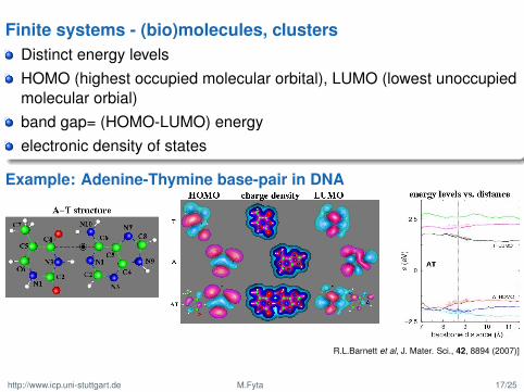
Finite systems - (bio)molecules, clustersDistinct energy levelsHOMO (highest occupied molecular orbital), LUMO (lowest unoccupiedmolecular orbial)band gap= (HOMO-LUMO) energyelectronic density of states

Example: Adenine-Thymine base-pair in DNA

R.L.Barnett et al, J. Mater. Sci., 42, 8894 (2007)]


Electronic structureProbability distribution of electrons in chemical systemsState of motion of electrons in an electrostatic field created by the nucleiExtraction of wavefunctions and associated energies through theSchrödinger equation:

i~∂

∂tΨ = HΨ time − dependent

EΨ = HΨ time − independent

Solves for:bonding and structureelectronic, magnetic, and optical properties of materialschemistry and reactions.


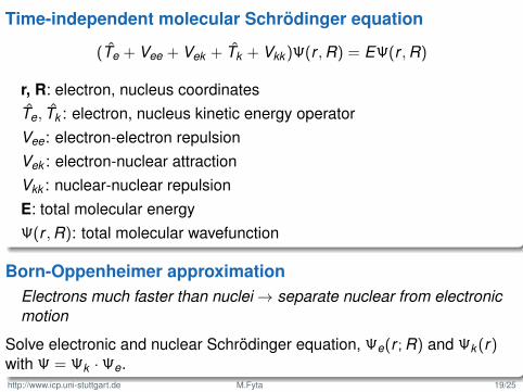
Time-independent molecular Schrödinger equation

(Te + Vee + Vek + Tk + Vkk )Ψ(r ,R) = EΨ(r ,R)

r, R: electron, nucleus coordinatesTe, Tk : electron, nucleus kinetic energy operatorVee: electron-electron repulsionVek : electron-nuclear attractionVkk : nuclear-nuclear repulsionE: total molecular energyΨ(r ,R): total molecular wavefunction

Born-Oppenheimer approximationElectrons much faster than nuclei→ separate nuclear from electronicmotion

Solve electronic and nuclear Schrödinger equation, Ψe(r ; R) and Ψk (r)with Ψ = Ψk ·Ψe.http://www.icp.uni-stuttgart.de M.Fyta 19/25

Approximations in electronic structure methods

Common approximations:in the Hamiltonian, e.g. changing from a wavefunction-based to adensity-based description of the electronic interactionsimplification of the electronic interaction termin the description of the many-electron wavefunction

Often the electronic wavefunction of a system is expanded in terms ofSlater determinants, as a sum of anti-symmetric electron wavefunctions:

Ψel(~r1, s1, ~r2, s2, ..., ~rN , sN) =∑m1,m2,...,mN

Cm1,m2,...,mN |φm1(~r1, s1)φm2(~r2, s2)...φmN ( ~rN , sN)|

where ~ri , s1 the cartesian coordinates and the spin components. Thecomponents φmN ( ~rN , sN) are one-electron orbitals.


Basis-setsChoices

Bulk systems: plane wavesMolecules/finite systems: atomic-like orbitals

Finite basis setThe smaller the basis, the poorer the representation, i.e. accuracy ofresultsThe larger the basis, the larger the computational load.Minimum basis sets:

only atomic orbitals containing all electrons of neutral atom, e.g. for H onlys-function, for 1st -row of periodic table, two s-functions (1s and 2s) and oneset of p-functions (2px , 2py , 2pz).

Improvementsdouble all functions: Double Zeta (DZ) basistriple all functions: Triple Zeta (TZ) basispolarization functions (higher angular momentum functions)mixed basis-sets, contracted basis-sets (3-21G, 6-31G, 6-311G, ...).


Basis-setsPlane-waves

Periodic functionsBloch’s theorem for periodic solids: φmN ( ~rN , sN) = un,k (~r)exp(i~k ·~r)

Periodic u expanded in plane waves with expansion coefficientsdepending on the reciprocal lattice vectors:

un,k (~r) =∑

|~G|≤|Gmax

cnk (~G)exp(i ~G ·~r)

Atomic-like orbitalsφmN ( ~rN , sN) =

∑n Dnmχn(~r)

Gaussian-type orbitals:

χζ,n,l,m(r , θ, φ) = NYl,m(θ, φ)r2n−2−lexp(−ζr2)

χζ,lx ,ly ,lz (x , y , z) = Nx lx y ly z lz exp(−ζr2)

the sum lx , ly , lz determines the orbital.http://www.icp.uni-stuttgart.de M.Fyta 22/25

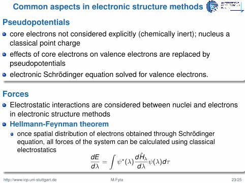
Common aspects in electronic structure methods

Pseudopotentialscore electrons not considered explicitly (chemically inert); nucleus aclassical point chargeeffects of core electrons on valence electrons are replaced bypseudopotentialselectronic Schrödinger equation solved for valence electrons.

ForcesElectrostatic interactions are considered between nuclei and electronsin electronic structure methodsHellmann-Feynman theorem

once spatial distribution of electrons obtained through Schrödingerequation, all forces of the system can be calculated using classicalelectrostatics

dEdλ

=

∫ψ?(λ)

dHλdλ

ψ(λ)dτ


Optimization: wavefunctions and geometriesnumerical approximations of the wavefunction by successive iterationsvariational principle, convergence by minimizing the total energy:

E ≤ 〈Φ|H|Φ〉

geometry optimization: nuclear forces computed at the end ofwavefunction optimization processnuclei shifted along direction of computed forces→ newwavefunction(new positions)process until convergence: final geometry corresponds to globalminimum of potential surface energy

Self consistent field (SCF)Particles in the mean field created by the other particlesFinal field as computed from the charge density is self-consistent withthe assumed initial fieldequations almost universally solved through an iterative method.


ab initio methods

Solve Schrödinger’s equation associated with the Hamiltonian of thesystemab initio (first-principles): methods which use established laws ofphysics and do not include empirical or semi-empirical parameters;derived directly from theoretical principles, with no inclusion ofexperimental data

Popular ab initio methodsHartree-FockDensity functional theoryMøller-Plesset perturbation theoryMulti-configurations self consistent field (MCSCF)Configuration interaction (CI), Multi-reference configuration interactionCoupled cluster (CC)Quantum Monte CarloReduced density matrix approaches


lecture notes - institute for computational physics - universit¤t

Documents