Computational Physics in the New Physics Degrees at Portsmouth

Chris Dewdney

Director of Undergraduate Studies

Reader in Theoretical Physics

Chris.Dewdney@port.ac.uk

Physics at Portsmouth?

• Physics delivered at Portsmouth since the 1960’s

• New BSc Applied Physics – started 2010

• MPhys Applied Physics, MPhys/BSc Physics, Astrophysics and Cosmology starting September 2015

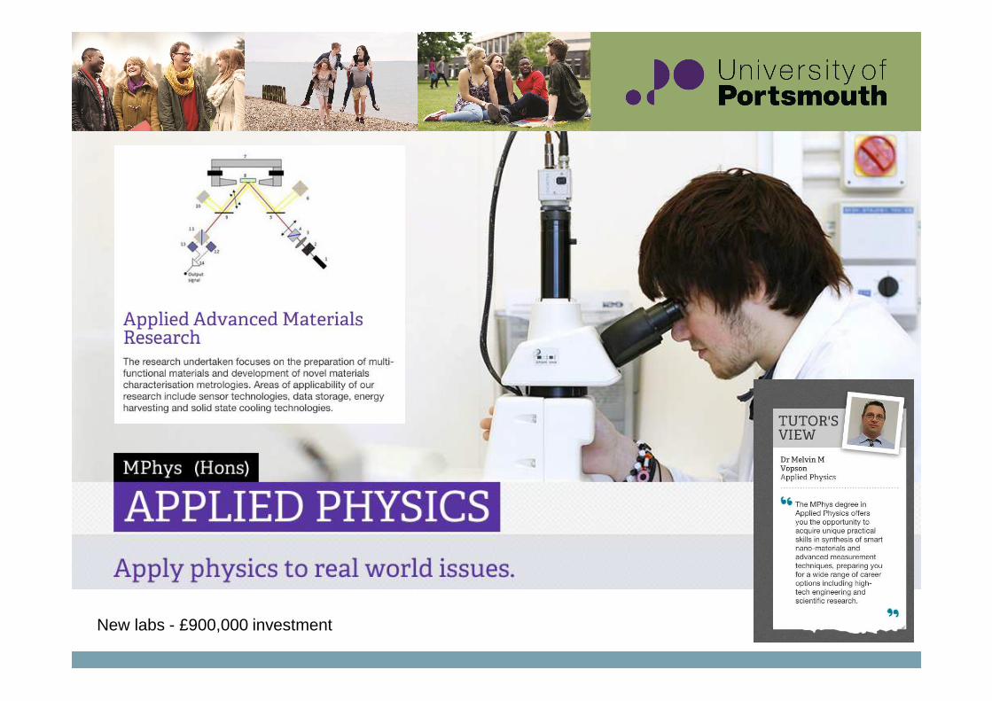
New labs - £900,000 investment

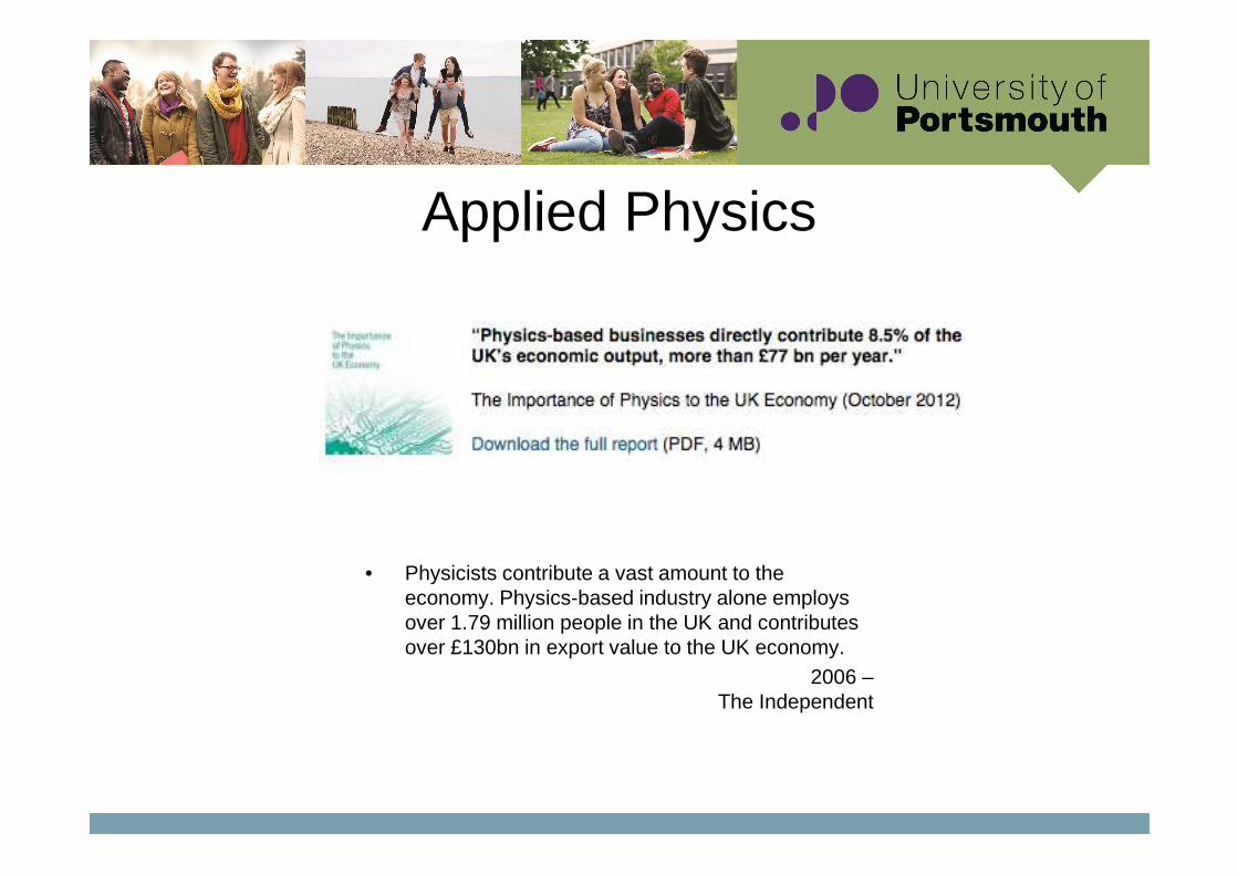
Applied Physics

• Physicists contribute a vast amount to the economy. Physics-based industry alone employs over 1.79 million people in the UK and contributes over £130bn in export value to the UK economy.

2006 –The Independent

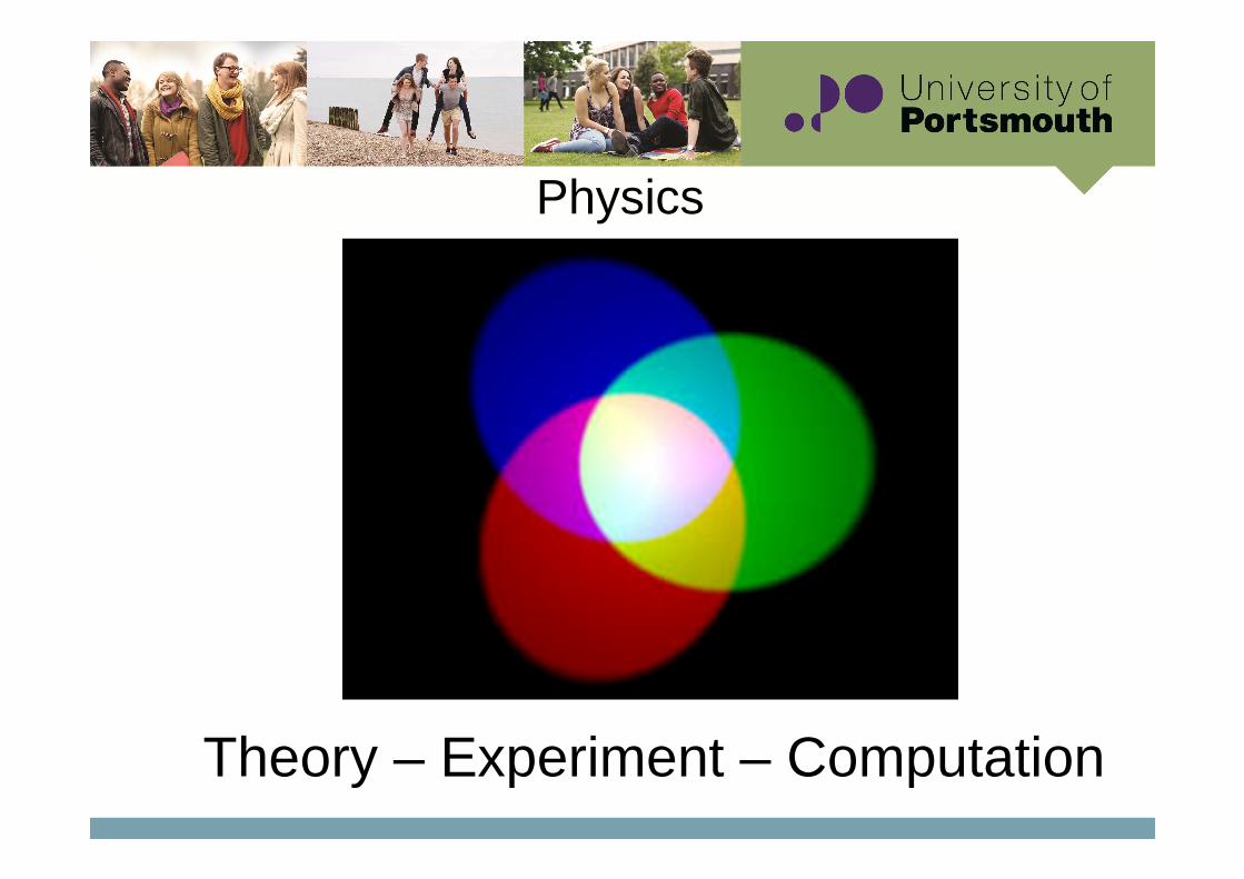
Theory – Experiment – Computation

Physics

Physics

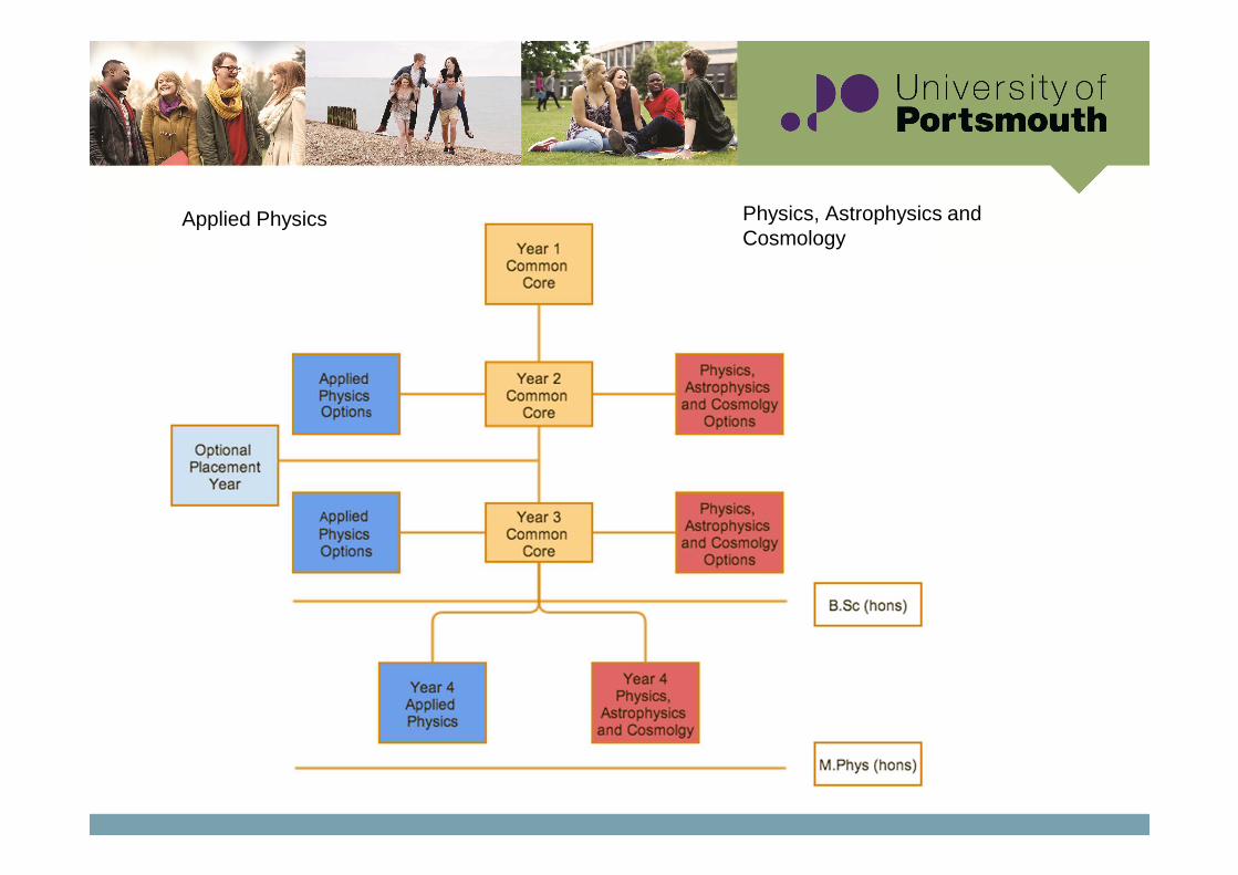
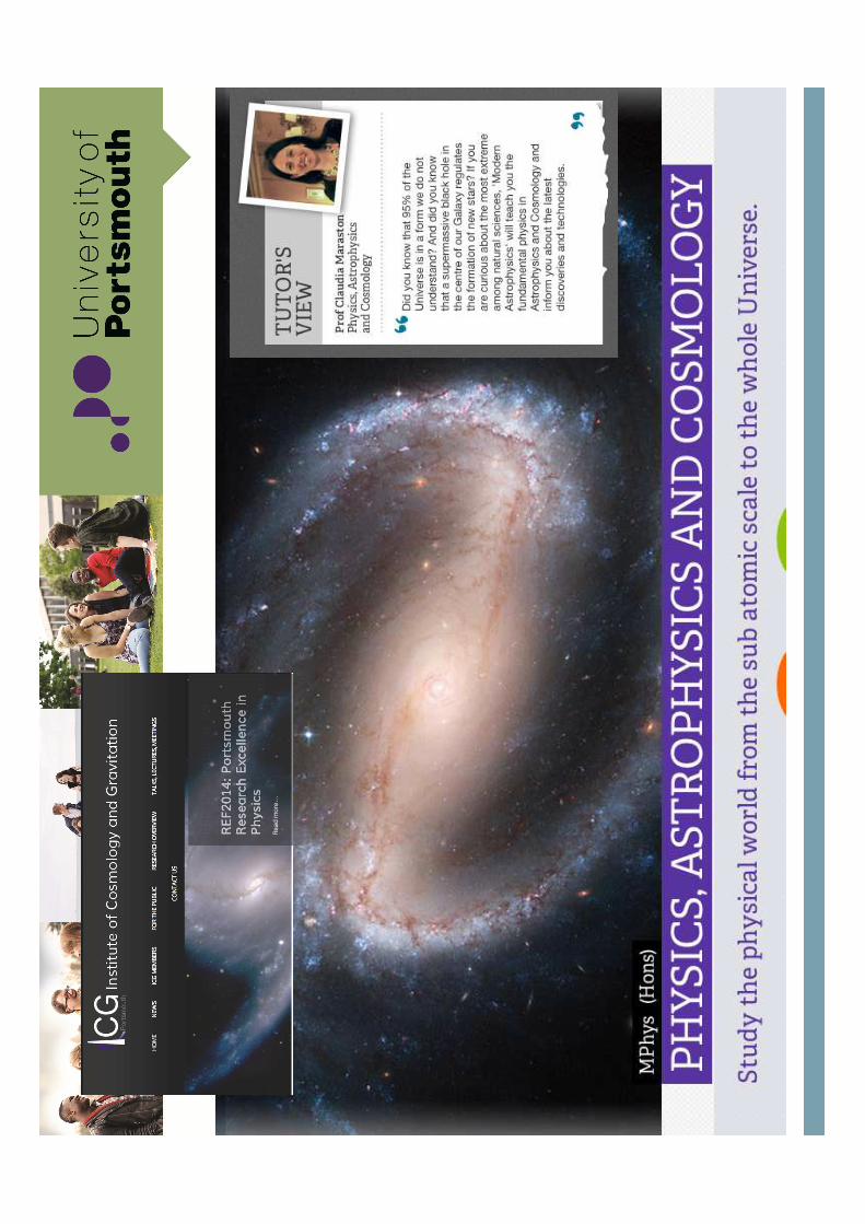
Physics, Astrophysics and Cosmology

Applied Physics

Adoption of Good Practice in HE (HEG,IOP, HESTEM,HEA)

8

Informed by Employers – Industry, Defence, Health Care and Commerce

9

� Vital participation of industry (Industrial Advisory

Board)

� Embed employability skills

� Develop students as independent and cooperative

learners

� Integrate understanding principles of physics with

mathematical/computational modelling laboratory

work through problem-based learning.

� Develop professional practice

Underdeveloped items

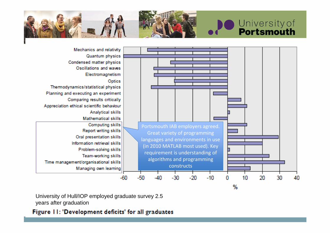
• Time-management and organisational skills (35%)*

• Oral presentation (29%)• Team working (25%)• Information retrieval (20%)* • Managing own learning (13%) *• Computing skills (12%) *• Ethical behaviour (12%)

22 July 2015

Portsmouth IAB employers agreed.

Great variety of programming

languages and environments in use

(in 2010 MATLAB most used). Key

requirement is understanding of

algorithms and programming

constructs

University of Hull/IOP employed graduate survey 2.5 years after graduation

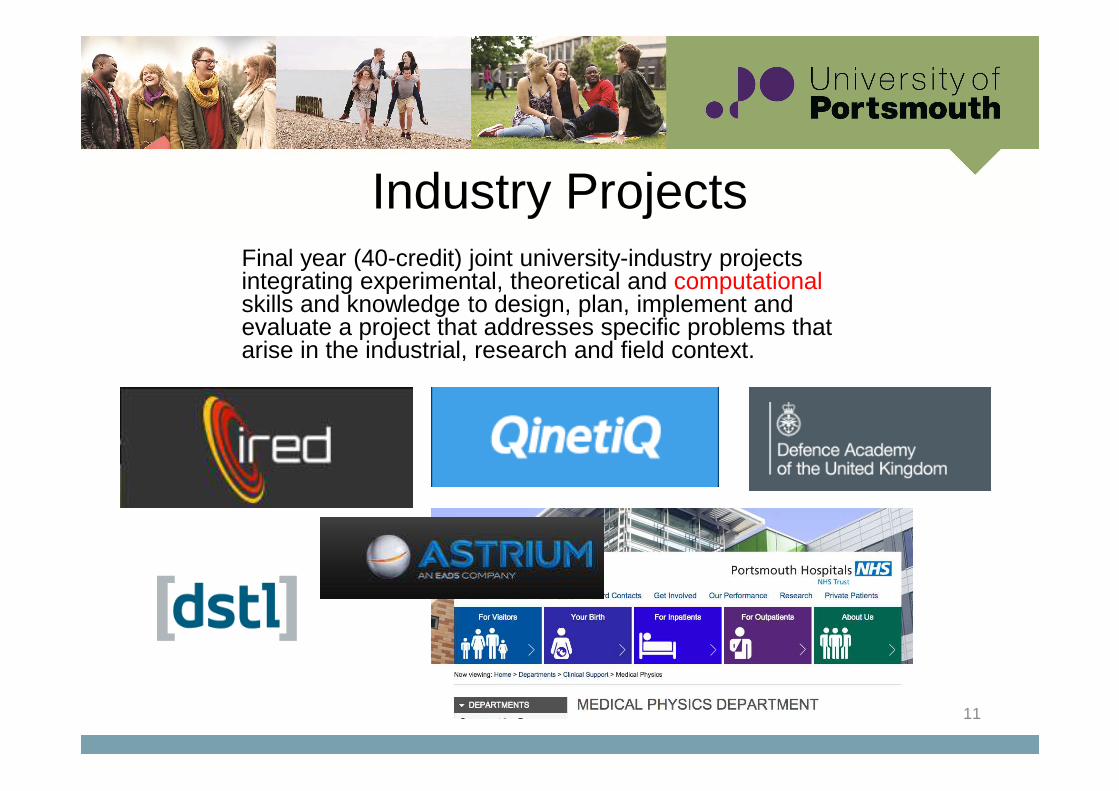
Industry ProjectsFinal year (40-credit) joint university-industry projects integrating experimental, theoretical and computationalskills and knowledge to design, plan, implement and evaluate a project that addresses specific problems that arise in the industrial, research and field context.

11

•IOP support–Higher Education Group–New Degrees Group (Liverpool, Portsmouth,

Salford, Leicester, Bradford, St Mary’s(Twickenham))

–Industry Group Projects

•HESTEM–Curriculum Development Group–Mathematical Modelling and Problem Solving Group (Mike Savage, Leeds)

–Problem-based Learning Laboratories Adopters (Derek Raine, Leicester)

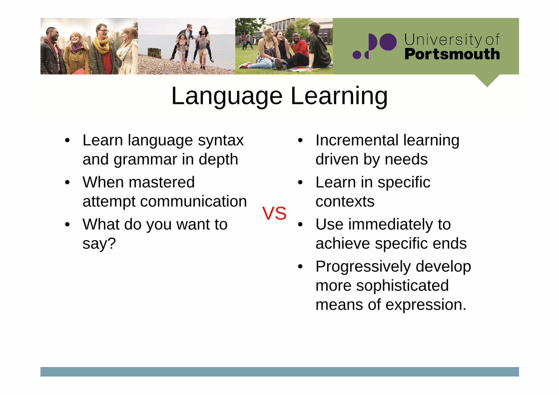
Language Learning

• Learn language syntax and grammar in depth

• When mastered attempt communication

• What do you want to say?

• Incremental learning driven by needs

• Learn in specific contexts

• Use immediately to achieve specific ends

• Progressively develop more sophisticated means of expression.

VS

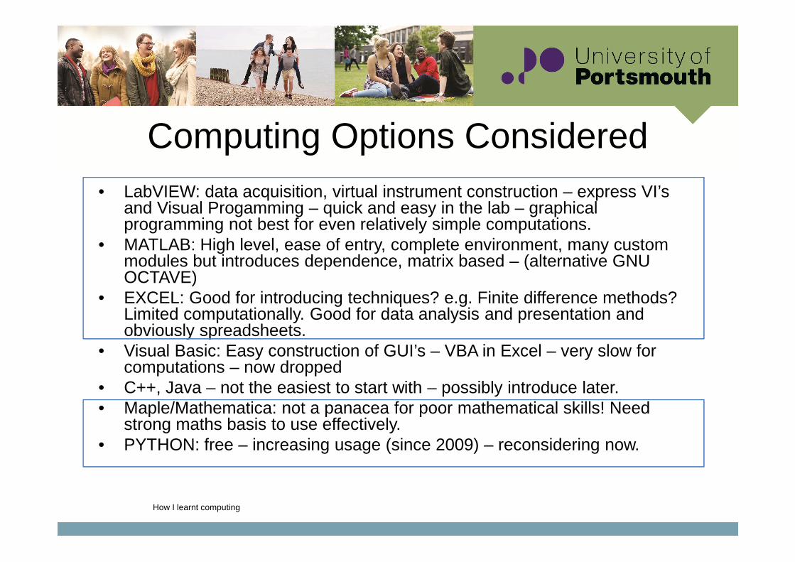
Computing Options Considered• LabVIEW: data acquisition, virtual instrument construction – express VI’s

and Visual Progamming – quick and easy in the lab – graphical programming not best for even relatively simple computations.

• MATLAB: High level, ease of entry, complete environment, many custom modules but introduces dependence, matrix based – (alternative GNU OCTAVE)

• EXCEL: Good for introducing techniques? e.g. Finite difference methods? Limited computationally. Good for data analysis and presentation and obviously spreadsheets.

• Visual Basic: Easy construction of GUI’s – VBA in Excel – very slow for computations – now dropped

• C++, Java – not the easiest to start with – possibly introduce later.• Maple/Mathematica: not a panacea for poor mathematical skills! Need

strong maths basis to use effectively.• PYTHON: free – increasing usage (since 2009) – reconsidering now.

How I learnt computing

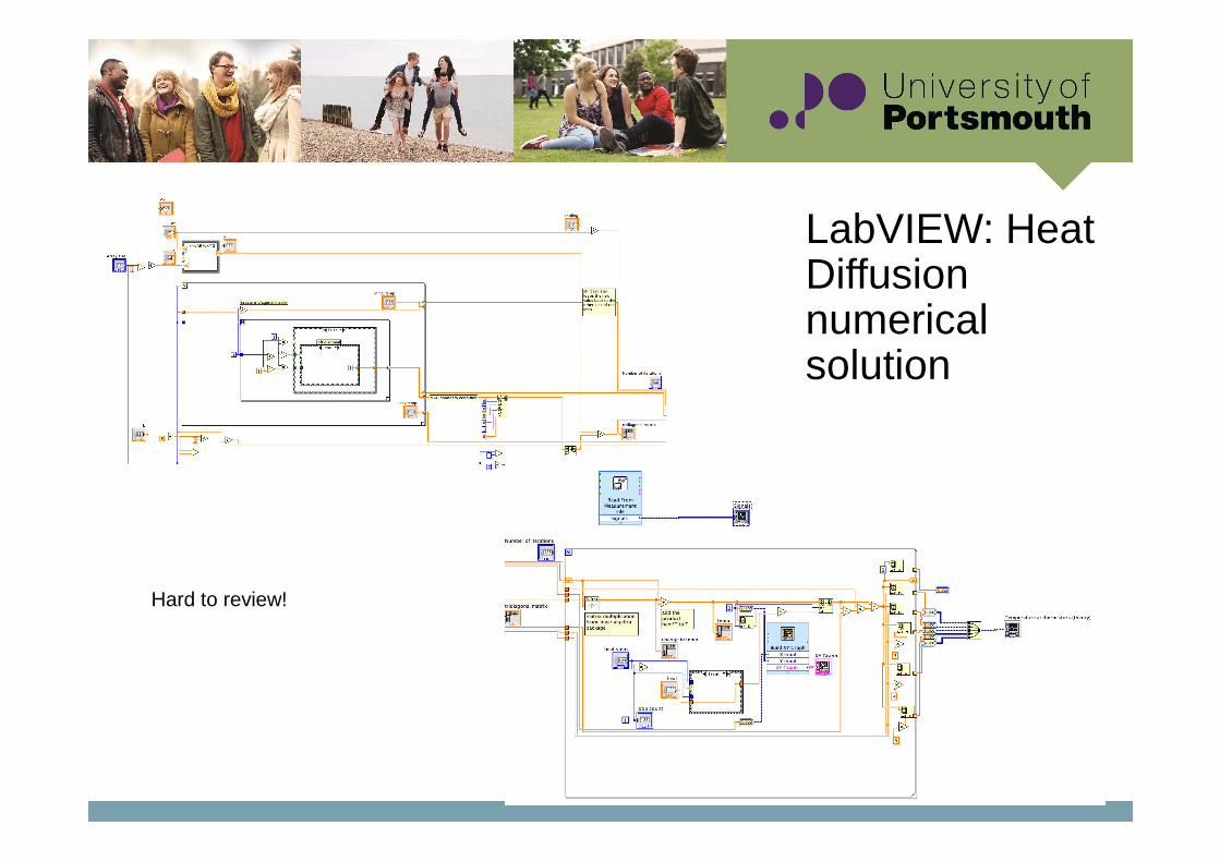
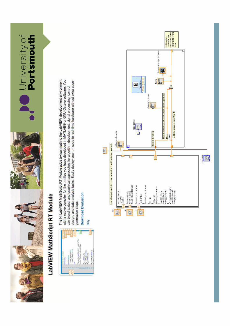
LabVIEW: Heat Diffusion numerical solution

Hard to review!

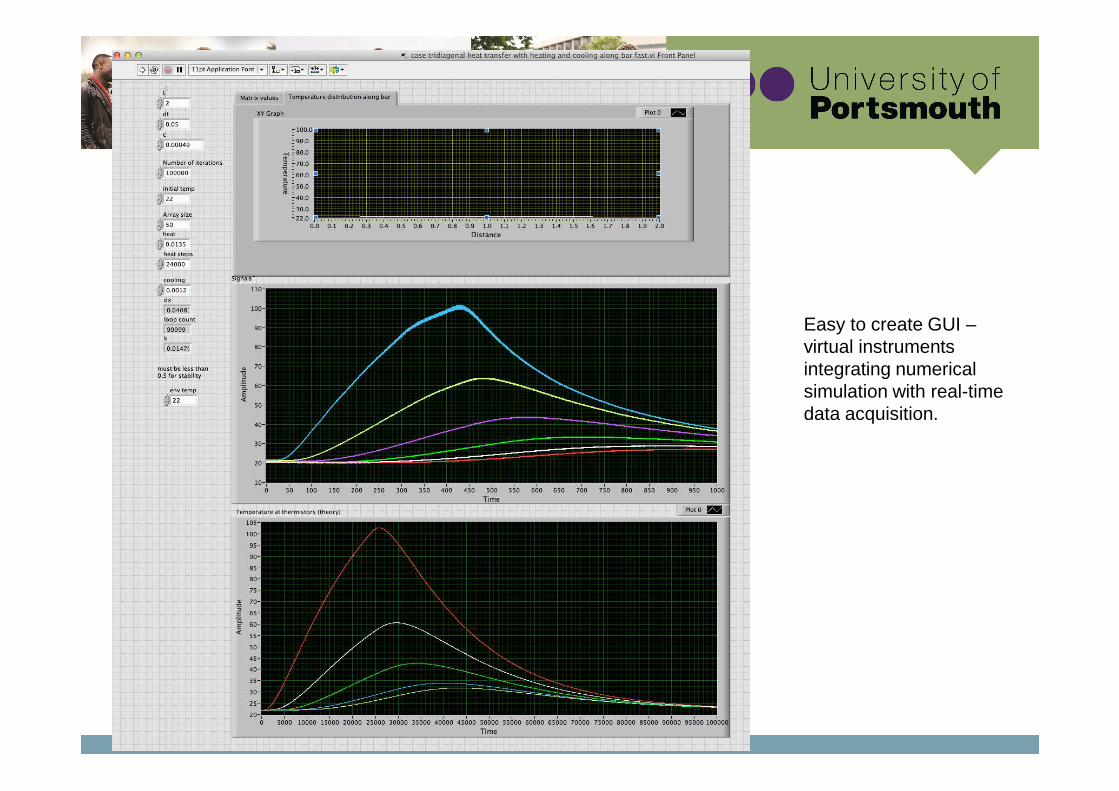
Easy to create GUI –virtual instruments integrating numerical simulation with real-time data acquisition.

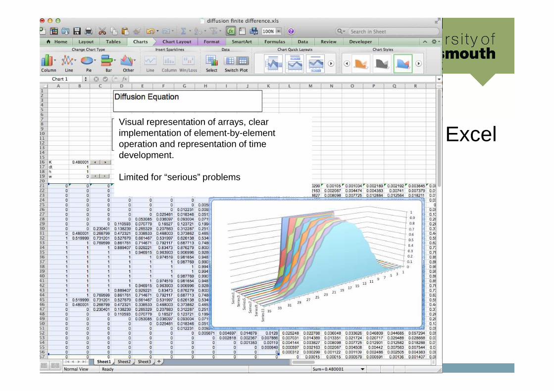
ExcelVisual representation of arrays, clear implementation of element-by-element operation and representation of time development.

Limited for “serious” problems

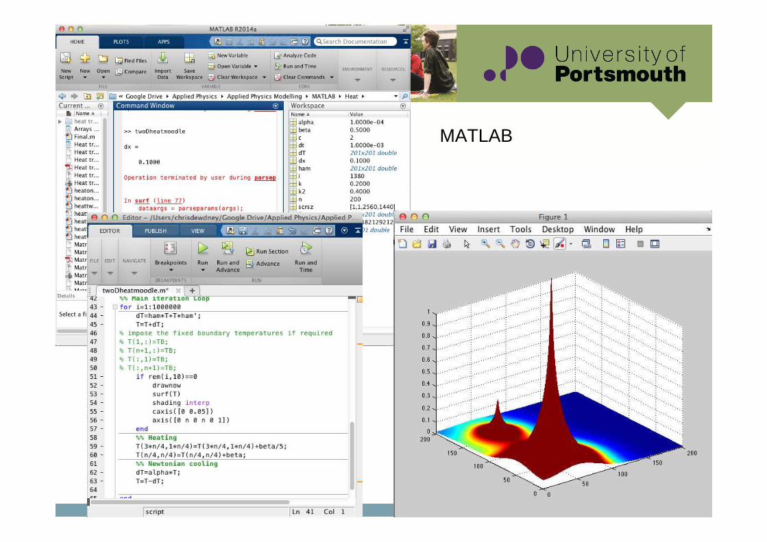
MATLAB

Computational Units and Integration in the Curriculum

• Level 4 Introduction to Computational physics

• Level 5 Computational Physics• Level 7 (MPhys) Advanced Computational

Techniques (2018-2019)

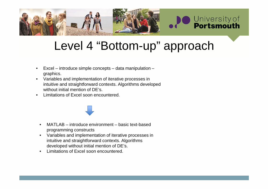
Level 4 “Bottom-up” approach

• Excel – introduce simple concepts – data manipulation –graphics.

• Variables and implementation of iterative processes in intuitive and straightforward contexts. Algorithms developed without initial mention of DE’s.

• Limitations of Excel soon encountered.

• MATLAB – introduce environment – basic text-based programming constructs

• Variables and implementation of iterative processes in intuitive and straightforward contexts. Algorithms developed without initial mention of DE’s.

• Limitations of Excel soon encountered.

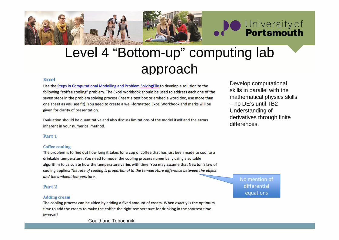
Level 4 “Bottom-up” computing lab approach

Develop computational skills in parallel with the mathematical physics skills – no DE’s until TB2Understanding of derivatives through finite differences.

No mention of

differential

equations

Gould and Tobochnik

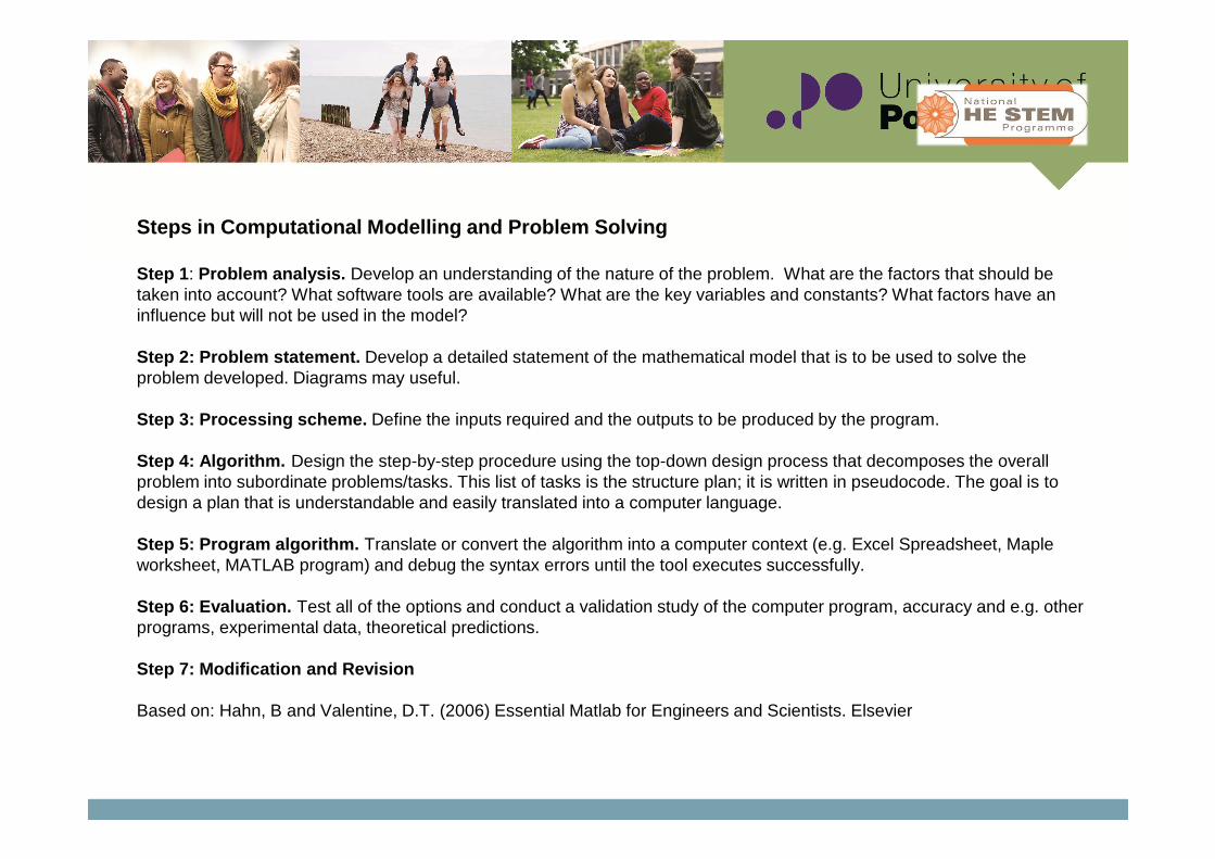
Steps in Computational Modelling and Problem Solving

Step 1: Problem analysis. Develop an understanding of the nature of the problem. What are the factors that should be taken into account? What software tools are available? What are the key variables and constants? What factors have an influence but will not be used in the model?

Step 2: Problem statement. Develop a detailed statement of the mathematical model that is to be used to solve the problem developed. Diagrams may useful.

Step 3: Processing scheme. Define the inputs required and the outputs to be produced by the program.

Step 4: Algorithm. Design the step-by-step procedure using the top-down design process that decomposes the overall problem into subordinate problems/tasks. This list of tasks is the structure plan; it is written in pseudocode. The goal is to design a plan that is understandable and easily translated into a computer language.

Step 5: Program algorithm. Translate or convert the algorithm into a computer context (e.g. Excel Spreadsheet, Maple worksheet, MATLAB program) and debug the syntax errors until the tool executes successfully.

Step 6: Evaluation. Test all of the options and conduct a validation study of the computer program, accuracy and e.g. other programs, experimental data, theoretical predictions.

Step 7: Modification and Revision

Based on: Hahn, B and Valentine, D.T. (2006) Essential Matlab for Engineers and Scientists. Elsevier

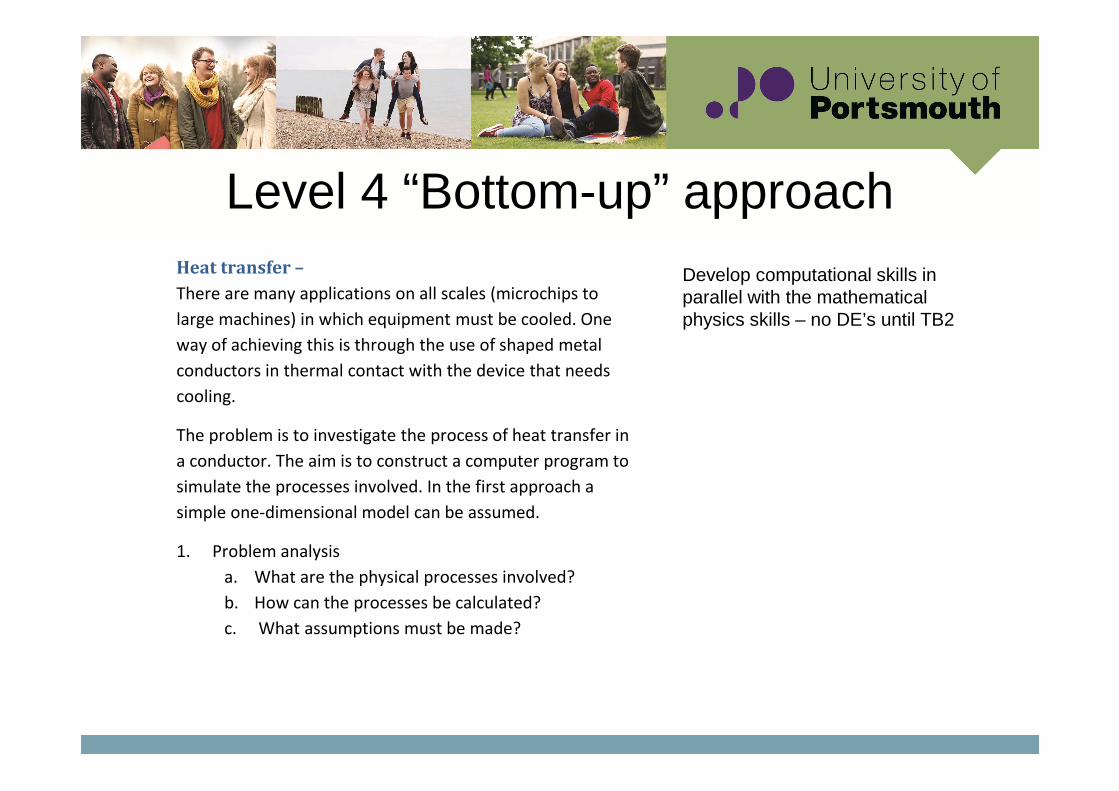
Level 4 “Bottom-up” approachHeat transfer –

There are many applications on all scales (microchips to

large machines) in which equipment must be cooled. One

way of achieving this is through the use of shaped metal

conductors in thermal contact with the device that needs

cooling.

The problem is to investigate the process of heat transfer in

a conductor. The aim is to construct a computer program to

simulate the processes involved. In the first approach a

simple one-dimensional model can be assumed.

1. Problem analysis

a. What are the physical processes involved?

b. How can the processes be calculated?

c. What assumptions must be made?

Develop computational skills in parallel with the mathematical physics skills – no DE’s until TB2

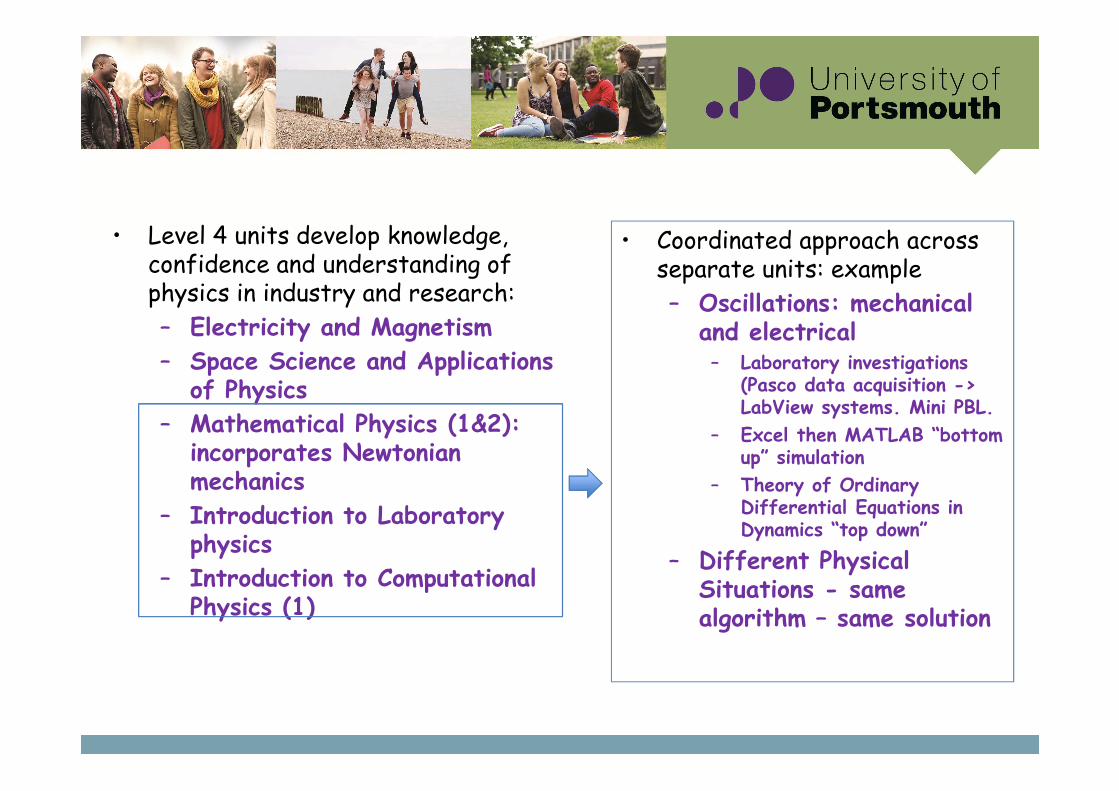
• Level 4 units develop knowledge, confidence and understanding of physics in industry and research:

– Electricity and Magnetism

– Space Science and Applications of Physics

– Mathematical Physics (1&2): incorporates Newtonian mechanics

– Introduction to Laboratory physics

– Introduction to Computational Physics (1)

• Coordinated approach across separate units: example

– Oscillations: mechanical and electrical

– Laboratory investigations (Pasco data acquisition -> LabView systems. Mini PBL.

– Excel then MATLAB “bottom up” simulation

– Theory of Ordinary Differential Equations in Dynamics “top down”

– Different Physical Situations - same algorithm – same solution

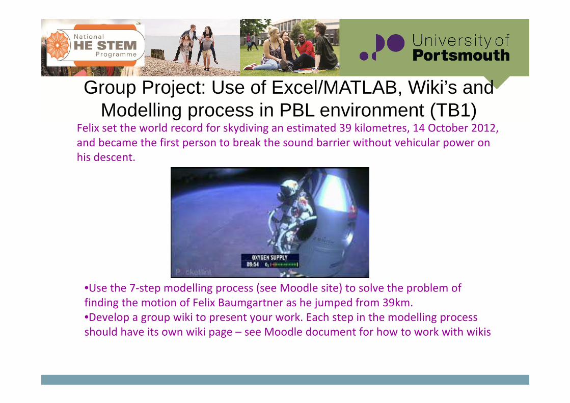
Group Project: Use of Excel/MATLAB, Wiki’s and Modelling process in PBL environment (TB1)

•Use the 7-step modelling process (see Moodle site) to solve the problem of

finding the motion of Felix Baumgartner as he jumped from 39km.

•Develop a group wiki to present your work. Each step in the modelling process

should have its own wiki page – see Moodle document for how to work with wikis

Felix set the world record for skydiving an estimated 39 kilometres, 14 October 2012,

and became the first person to break the sound barrier without vehicular power on

his descent.

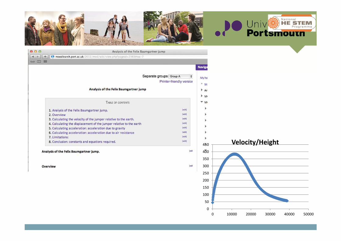
0

50

100

150

200

250

300

350

400

450

0 10000 20000 30000 40000 50000

Velocity/Height

• Level 5 Core:

– Laboratory-based PBL

– Thermodynamics and Statistical Physics

– Computational Physics

– Quantum, Atomic and Nuclear

– Mathematical Physics

– Waves and Optics

– Heat transfer– Laboratory investigations

LabView systems. PBL.

– MATLAB “bottom up” simulation – finite difference

– Theory of Ordinary Differential Equations in Dynamics “top down”

– Solving problems in QM using Maple

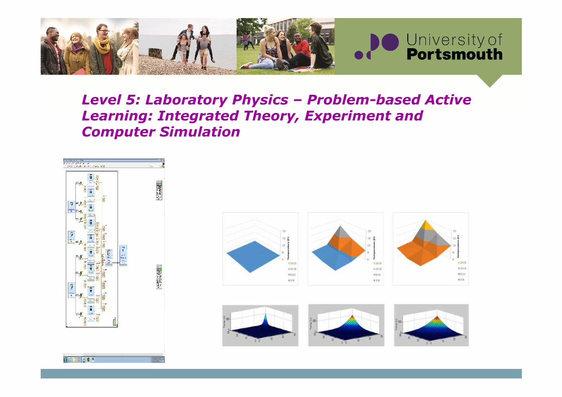
Level 5: Laboratory Physics – Problem-based Active Learning: Integrated Theory, Experiment and Computer Simulation

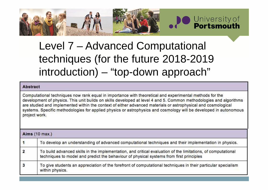
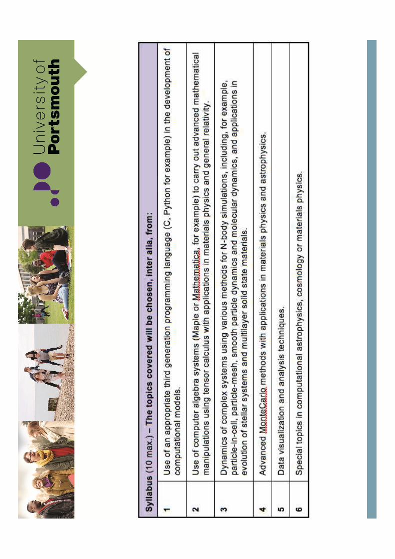
Level 7 – Advanced Computational techniques (for the future 2018-2019 introduction) – “top-down approach”

Effectiveness and Evaluation?

•Need a systematic assessment and evaluation

–Excel -> Matlab ?–Problem-based approach – a diversion from learning computing techniques systematically?

–Integrated maths/labs/physics/computing PBL’s?

• Perhaps a basis for a collaborative project?