journal of computational physics - cornell university of computational physics 294 (2015) 110–126...

Journal of Computational Physics 294 (2015) 110–126

Contents lists available at ScienceDirect

Journal of Computational Physics

www.elsevier.com/locate/jcp

Specific volume coupling and convergence properties

in hybrid particle/finite volume algorithms for turbulent

reactive flows

Pavel P. Popov a,∗, Haifeng Wang b, Stephen B. Pope c

a University of California – Irvine, United Statesb Purdue University, United Statesc Cornell University, United States

a r t i c l e i n f o a b s t r a c t

Article history:Received 5 December 2014Accepted 3 March 2015Available online 17 March 2015

Keywords:Turbulent reactive flowPDF methods for subgrid closureSpecific volume couplingLagrangian Monte Carlo simulationHybrid particle/finite volume algorithms

We investigate the coupling between the two components of a Large Eddy Simulation/Probability Density Function (LES/PDF) algorithm for the simulation of turbulent reacting flows. In such an algorithm, the Large Eddy Simulation (LES) component provides a solution to the hydrodynamic equations, whereas the Lagrangian Monte Carlo Probability Density Function (PDF) component solves for the PDF of chemical compositions. Special attention is paid to the transfer of specific volume information from the PDF to the LES code: the specific volume field contains probabilistic noise due to the nature of the Monte Carlo PDF solution, and thus the use of the specific volume field in the LES pressure solver needs careful treatment. Using a test flow based on the Sandia/Sydney Bluff Body Flame, we determine the optimal strategy for specific volume feedback. Then, the overall second-order convergence of the entire LES/PDF procedure is verified using a simple vortex ring test case, with special attention being given to bias errors due to the number of particles per LES Finite Volume (FV) cell.

© 2015 Elsevier Inc. All rights reserved.

1. Introduction

The PDF method for the treatment of turbulent reactive flows [1,2] has been shown to be highly effective, due to the fact that the chemical source term, which is highly non-linear in a combustion application, appears in closed form and thus requires no modeling [3]. Initially, the PDF methodology was coupled to Reynolds-Averaged Navier–Stokes (RANS) hydrodynamic solvers, thus giving rise to the RANS/PDF class of algorithms for simulation of turbulent reactive flows, which are to this date effectively used in simulating combustion processes (see [3] for a review). We note that there are three main classes of computationally tractable algorithms for approximating the composition PDF [3]. Here we focus on the Lagrangian Particle Monte Carlo class, in which the PDF is approximated from an ensemble of points (from here on referred to as “particles”) that are advected and diffused in physical space according to the LES resolved velocity and turbulent diffusivity [1,9] (in this paper, we use the terms “turbulent viscosity” and “turbulent diffusivity” to denote the viscosity and diffusivity used to model the turbulent motions unresolved by the LES grid). In the related Eulerian Particle Monte Carlo method [22], the locations of particles are fixed to the grid nodes. Yet another class of PDF algorithms, the Eulerian Field Monte Carlo

* Corresponding author.E-mail address: [email protected] (P.P. Popov).

http://dx.doi.org/10.1016/j.jcp.2015.03.0010021-9991/© 2015 Elsevier Inc. All rights reserved.

http://dx.doi.org/10.1016/j.jcp.2015.03.001

http://www.ScienceDirect.com/

http://www.elsevier.com/locate/jcp

mailto:[email protected]

http://dx.doi.org/10.1016/j.jcp.2015.03.001

http://crossmark.crossref.org/dialog/?doi=10.1016/j.jcp.2015.03.001&domain=pdf

P.P. Popov et al. / Journal of Computational Physics 294 (2015) 110–126 111

class [21,20,8], instead employs an ensemble of composition fields defined over the entire domain, which evolve by partial differential equations with a stochastic forcing component. All of these approaches have their strengths and differences [3]: for example, the Lagrangian Particle Monte Carlo approach allows for more accurate treatment of sub-filter mixing and diffusion [6]. With increasing computational resources, the Large Eddy Simulation (LES) approach for turbulence modeling has been supplanting RANS as the hydrodynamic solver used for turbulent combustion simulations [17]. First introduced by Pope [16], hybrid Large Eddy Simulation/Probability Density Function (LES/PDF) methods have the added benefit that the LES approach eliminates the need for modeling of the large scale turbulent motions, which are highly geometry-dependent and fall outside of the scope of the Kolmogorov hypotheses [2]. Hybrid LES/PDF methods have been demonstrated to be highly effective in simulating laboratory-scale flames [9–11,18].

In a typical LES/PDF simulation, the LES code provides fields of velocity and turbulent diffusivity to the PDF code. The PDF code then transports the particles in physical space, performs molecular diffusion and mixing, and chemical reaction steps, and then passes back to the LES code the fields of specific volume, molecular viscosity and diffusivity. The very different nature of the two components of an LES/PDF algorithm poses serious challenges for the implementation of information transfer between the stochastic PDF code, whose fields contain considerable random errors, and the LES code, which is a straightforward Finite Volume (FV) algorithm, employing discretization schemes which assume a certain level of regularity from the fields on which they operate. Here, we examine in detail this interplay between the LES and PDF components. Particular emphasis is given to the feedback of specific volume from PDF to LES. In advancing the hydrodynamic variables, the LES code solves a Poisson equation for pressure, whose source term contains the rate of change of specific volume. Since specific volume information is obtained from the stochastic PDF code, special effort must be made to ensure that the specific volume fields which are input into the LES pressure solver contain as little statistical error as possible. Furthermore, it is desired that the overall LES/PDF time stepping procedure be second-order accurate in space and time. In the context of the LES/PDF code developed by the Turbulence and Combustion Group at Cornell University [18], we address these two issues, examining different strategies in performing PDF to LES feedback, and testing the overall order of convergence of the LES/PDF code. We note that certain PDF algorithms for reactive flows, such as the direct quadrature method of moments introduced by Fox [24] are deterministic in nature and as such lack the complication of statistical noise in the PDF volume information. On the other hand, stochastic PDF solution algorithms such as the ones dealt with here are computationally more efficient for high-dimensional sample spaces, such as are encountered in LES/PDF simulations with detailed chemistry tracking tens or even hundreds of species.

While a lot of the computational algorithms for LES/PDF, and their solutions, have evolved from prior work on the more venerable RANS/PDF class of codes, specific volume coupling does not present as big of a computational challenge in a RANS/PDF context as it does in LES/PDF, because the former allows for the evaluation of statistics over long time intervals, which reduces the stochastic noise which is the main obstacle in specific volume coupling. We note that specific volume feedback from PDF to LES has previously been addressed as a component of an overall algorithm for the simulation of turbulent reactive flows. Previous researchers have proposed specific volume coupling schemes based on direct evaluation from the particle ensemble [10] (analogous to the scheme PSV described in Section 3), and schemes based on extracting specific volume information from an auxiliary transported scalar (analogous to the scheme TSV described in Section 3), where the transported scalar is either enthalpy [13,12,4,11] or temperature [10]. While using a similar formulation at the PDE level for specific volume feedback, the present work extends the above studies by examining the LES to PDF coupling error in detail, isolating it from other sources of numerical errors in an LES/PDF algorithm, and determining the optimal coupling strategy. A further original contribution of the present work is in the development of an LES/PDF coupling algorithm which allows for second-order accuracy of the overall code (with respect to both the grid size and time step); this second-order convergence is then verified numerically. The optimal of the algorithms presented below has been successfully employed [23] in a series of simulations of the Sandia–Sydney HM series of bluff-body flames. While the subject of that paper was not specific volume coupling, its results confirm that the optimal coupling scheme determined in the present work is suitable for use in a realistic LES/PDF simulation.

The rest of this paper is organized as follows: in Section 2, we present the equations solved by an LES/PDF algorithm for turbulent reactive flows. Section 3 describes in detail the issues that arise in the coupling of the LES and PDF algorithms; two alternative approaches for specific volume coupling are outlined. The numerical algorithms for coupling between the LES and PDF codes are described in Section 4. Numerical tests of these couplings are performed in Sections 5 and 6, in which the fully-coupled LES/PDF implementations are tested against a Standalone-LES (S-LES) code with no coupling errors. Section 5 describes results from a long time interval turbulent jet flow, representative of a typical LES/PDF simulation. In Section 6, we show convergence results from a simple vortex ring numerical test case, which demonstrates that the overall LES/PDF algorithm is second-order accurate in space and time.

2. Equations solved by the LES/PDF algorithm

In this section, we present the equations which are solved by an LES/PDF algorithm. Throughout the present paper we use a tilde to denote mass weighted resolved quantities (also referred to here as Favre-averaged quantities) solved for by the LES/PDF solver, e.g. u for the mass-weighted resolved velocity vector, and φ for the mass-weighted resolved composition vector. Additionally, the composition PDF solver computes the evolution of individual particle properties, which we denote by a star superscript, e.g. φ∗

α for the α-component of an individual particle’s composition vector.

112 P.P. Popov et al. / Journal of Computational Physics 294 (2015) 110–126

In the present study, we use a simple flamelet chemistry model [19], and the composition vector φα consists of a single component, the mixture fraction. This still allows for considerable specific volume variation throughout the flow, which is necessary for testing the specific volume coupling. Furthermore, using a mixture-fraction-only composition vector enables us to perform simulations of the same flow via both LES/PDF and standalone-LES methods, with both solutions evolving by the same governing equations. This allows us to approximate the LES/PDF coupling error as the difference between the standalone-LES and the LES/PDF solutions.

First, we describe the governing equations for a standalone-LES simulation with flamelet chemistry modeling. The LES governing equations are the same as those used by Pierce and Moin [7] (with the exception that in [7] the authors also use a progress variable in the flamelet model), by Wang and Pope [18], and by Kemenov et al. [19].

2.1. Governing equations for a standalone-LES simulation

We denote by u j, ξ, ξ2, respectively, the Favre-averaged LES velocity, mixture fraction and square of mixture fraction. The Favre-averaged molecular viscosity and diffusivity are denoted as ν and D , and their turbulent counterparts are νT , DTrespectively. The turbulent viscosity, νT , is evaluated by the dynamic Smagorinsky procedure, and the turbulent diffusivity, DT , is determined by using a specified value for the turbulent Schmidt number:

νT

DT= σT , σT = 0.4. (1)

Finally, we denote with p, ρ , respectively, the LES resolved pressure and density. With these definitions, the variable-density incompressible standalone-LES code solves the following set of equations

∂ρ

∂t+ ∂ρu j

∂x j= 0, (2)

∂(ρu j

)∂t

+ ∂(ρui u j)

∂xi= − ∂ p

∂x j+ 2

∂

∂xi

(ρ (ν + νT )

(S i j − 1

3Skkδi j

)), (3)

∂(ρξ)

∂t+ ∂

(ρu j ξ

)∂x j

= ∂

∂x j

(ρ(

D + DT) ∂ξ

∂x j

), (4)

∂(ρξ2

)∂t

+∂(ρu j ξ

2)

∂x j= ∂

∂x j

(ρ(

D + DT) ∂ξ2

∂x j

)+ Sξ2 . (5)

Eqs. (2)–(5) are respectively the Favre-averaged forms of the continuity, momentum, and scalar evolution equations for the mixture fraction, ξ , and its square ξ2. We note that in the numerical implementation of the mixture fraction model by the LES code, realizability in mixture fraction space is enforced when the material properties are retrieved from a flame table for the mixture fraction and its variance. The tensor Sij is the resolved strain rate, whereas the scalar Sξ2 is a source term in the scalar evolution equation for ξ2, determined by the scalar mixing model. For the present study, which uses the dynamic Smagorinsky procedure, we denote by the Smagorinsky filter size, and the exact form of Sξ2 is:

Sξ2 = −2ρ D∂ξ

∂xi

∂ξ

∂xi− 2ρ�

(ξ2 − ξ2

), (6)

� = DT + 2D

2, (7)

where the quantity � is known as the mixing frequency [9].In the flamelet chemistry approach, the material properties ρ, ν, D are functions of ξ and ξ2 only, the latter two via the

resolved temperature, T

ρ = ρ(ξ, ξ2

), (8)

T = T(ξ, ξ2

), (9)

ν = ν0

(T

300[K])1.69

,ν

D= σ , σ = 0.82, ν0 = 1.42 × 10−5

[m2

s

]. (10)

For most turbulent reactive flows with flamelet modeling, the form of the constitutive equations (Eqs. (8)–(10)) is tradi-tionally determined by performing a laminar opposing jet flame simulation, and assuming that the PDF of the mixture fraction, ξ , belongs to the β-function family. This then allows us to tabulate every moment of the PDF of ξ – in particular ρ, T – as a function of ξ , ξ2. However, in the present work we forgo the flamelet opposed jet solution: instead, we specify the temperature T and specific volume v as quadratic functions of the mixture fraction ξ :


v (ξ) = 7.98 − 23(ξ − 0.551)2[

m3

kg

], (11)

T (ξ) = 2100[K] − 7200[K](ξ − 0.5)2. (12)

Note that the temperature variation implies a stoichiometric mixture fraction of 0.5, which is considerably higher than the stoichiometric mixture fraction for a methane–air flame. The specification in Eq. (12) was chosen so that the temperature could vary from 300 K in the fuel and co-flow stream, to a maximum of 2100 K, while following a quadratic variation. As elaborated in Section 5, this is done so that the Favre-averaged values v and T are independent of the shape of the PDF of ξ . This allows for consistency between the self-contained solution of Eqs. (2)–(10) (which we shall refer to as a Standalone-LES (S-LES) solution), and the fully-coupled LES/PDF simulation (described in the remainder of this section and in Section 3) with a single scalar for mixture fraction. As seen in Sections 5 and 6, such consistency provides a useful numerical test case for examining the errors inherent to the LES to PDF coupling.

We note that, while the present chemistry formulation is considerably simplified when compared to a typical LES/PDF solution, it does feature a similar variation of the specific volume as a function of chemical composition. The specific volume function specified in Eq. (11) implies a factor of 8 difference between the specific volume of reactants and products. Therefore, the specific volume variance among the particles in a given cell is on the same order of magnitude as that which would be expected in an LES/PDF simulation with detailed chemistry. It is this variance, combined with the noise in the SDE by which the particle positions evolve, that generates the noise in the PDF specific volume fields. Therefore, the present specification of a chemical model, while much simpler than the detailed chemistry models used in LES/PDF, is adequate to test the implementation of specific volume coupling algorithms which are meant to be used in LES/PDF algorithms.

2.2. Governing equations for the LES component of an LES/PDF simulation

In an LES/PDF simulation, we remove the flamelet modeling from the standalone-LES simulation described in the previ-ous subsection, and replace it with composition PDF modeling of the reaction. Therefore, from all the governing equations of a standalone-LES simulation listed above, the LES component of an LES/PDF simulation solves only Eqs. (2), (3), (7), (10). This leaves the evaluation of resolved specific volume and temperature, which is done by the PDF component.

2.3. Governing equations for the PDF component of an LES/PDF simulation

The PDF code takes a Monte Carlo approach to approximating the mass-weighted composition PDF. The simulation domain is discretized into PDF cells, which consist of one or more LES FV cells [18], and, for a specified parameter Npc ,

each PDF cell contains between √

2N pc2 and

√2Npc particles. Each particle has a mass m∗ , which is unchanged unless that

particle is split in two or combined with another (for the purpose of controlling the number of particles in a PDF cell), and a location X∗

j and composition φ∗α . In the equations below, we use the superscript ∗ to denote either an individual particle’s

property (such as m∗ for the mass of the current particle), or the value of an LES field evaluated at that particle’s location (such as φ∗

α for the resolved mass weighted composition vector at the particle’s current location). With this notation, the evolution equations for X∗

j and φ∗α are:

dX∗j =[

u j + 1

ρ

∂(ρ DT

)∂x j

]∗dt +

[2D∗

T

]1/2dW ∗

j , (13)

dφ∗α = −�∗ (φ∗

α − φ∗α

)dt +

[1

ρ

∂

∂x j

(ρ D

∂φα

∂x j

)]∗dt + Sα

(φ∗)dt. (14)

In the above equations, � denotes the mixing frequency introduced in Eq. (7), and Sα(φ∗) is the reaction source term. The term dW ∗

j denotes a Wiener increment, with the star superscript emphasizing that the Wiener processes for the different particles are independent. Note that the diffusivity term in Eq. (13) is turbulent diffusivity only: this is done so that, in the limit as the LES filter decreases below the Kolmogorov lengthscale, and the simulation converges to a DNS solution, the composition PDF would appropriately converge to a Dirac delta function; the scalar diffusion due to molecular diffusivity is taken into account by the second term on the right-hand side of Eq. (14).

We shall use angled brackets, 〈·〉, to denote a sum over all particles in a given cell and its immediate neighbors, weighted by a basis function B(X∗

j ) whose support lies within the present cell and its neighbors: for a general particle property g , we have

〈g〉 =∑

cell+neighbors

g∗B(

X∗j

). (15)

The two most common examples for B(X∗j ) are the indicator function of the cell, whose use we shall refer to as the

Particle-in-Cell (PIC) approach and a linearly decreasing tent function which is centered at the cell’s center of mass, whose


use we shall refer to as the Cloud-in-Cell (CIC) approach [6]. The implementation of CIC is more difficult, since it involves additional communication in order to obtain information about the particles in the neighboring cells. However, CIC comes with the advantage that the continuous form of B(X∗

j ) implies that 〈g〉 is itself continuous in time, whereas for PIC there is a discontinuous jump in 〈g〉 as particles enter and leave the cell.

We also apply alternating direction implicit smoothing to the cell mean averages 〈g〉, and denote the smoothed fields as {〈g〉}. The smoothing process is described in detail in [6]. Here, we need only note that the amount of smoothing is controlled by a parameter, α, so that implicit smoothing with a given value of α is equivalent to explicit smoothing over αcells in each direction. The value α = 1.0 corresponds to no smoothing.

With this definition of a local ensemble mean, v, T are defined as

v ={ 〈mv〉

〈m〉}

, (16)

T ={ 〈mT 〉

〈m〉}

, (17)

where m∗, v∗, T ∗ respectively denote a particle’s mass, specific volume and temperature. The resolved viscosities and diffu-sivities are then defined by Eqs. (9), (10), as in the standalone-LES approach. Whereas in the standalone-LES approach, v, Tare functions of the mixture fraction only, in the LES/PDF approach, v, T are functions of the entire composition vector, φα . As already mentioned, in Sections 5 and 6 we use for our numerical tests a composition vector which consists only of the mixture fraction, for the purposes of comparing standalone-LES and LES/PDF solutions, which allows us to determine the amount of error in the simulation which is due to the LES/PDF coupling. However, it is important to note that in a typical LES/PDF simulation, the composition vector φα consists of the collection of significant chemical species, with the addition of enthalpy, and so there is no modeling involved in obtaining v and T from φα . This is one of the advantages of PDF reaction modeling over the flamelet approach. Another advantage is that the source term Sα(φ) on the right hand side of Eq. (14)requires no modeling either, provided that the chemical species to be used in the composition vector φα are appropriately chosen.

3. Coupling between the LES and PDF solutions

In the present LES/PDF algorithm, the LES algorithm uses resolved temperature values obtained from the PDF code, and the PDF code uses values for velocity, molecular and turbulent viscosity obtained from the LES code. Information about specific volume originates in the PDF code, but its transfer to the LES code is challenging, for the following reason: in the solution of the momentum and continuity equations, Eqs. (2), (3) by the LES solver, pressure is determined as the solution of a Poisson equation whose source includes the term ∂ v/∂t . Due to the stochastic nature of the PDF solution, however, (Eq. (13)) for a given time step t , the statistical error in the increment v , for a single-particle ensemble, is

εst1 = C1t1/2, (18)

where C1 is a fixed constant, proportional to D1/2T . Therefore, the statistical error in the smoothed increment v , with Npc

particles per cell [6], is

εst2 = C2t1/2(Npcα3

)1/2, (19)

and so the approximation

∂ v/∂t ≈ v/t (20)

contains a statistical error whose magnitude scales in the following manner

εst = C(Npcα3t

)1/2, (21)

where C is a constant which depends only on the flow geometry and material properties, N pc is the number of particles per cell and α is the smoothing parameter: note that since t appears in the denominator of Eq. (21), for small values of t the error implied by Eq. (21) is considerable.

In order to obtain a solution to the Poisson equation for pressure, we can take one of two alternative approaches for specific volume coupling.

3.1. The particle specific volume approach (PSV)

The PSV approach uses the straightforward procedure of simply passing the PDF values of specific volume to the LES code, and using a value for the smoothing parameter α which is large enough to reduce the error εst to manageable levels. As we see below, in the numerical tests of coupled LES/PDF turbulent jet simulations, this approach requires the use of smoothing parameter values as large as α = 4.0 (which implies that smoothing is performed over 64 cells). Overall, we show below that the PSV approach is not as accurate as the specific volume coupling approach which is described next.


3.2. The transported specific volume approach (TSV)

The Transported Specific Volume (TSV) approach is based on the fact that the change of resolved specific volume which is due to transport in physical space (Eq. (13)) can be calculated by the LES solver, thus leaving only the specific volume change due to turbulent mixing, molecular diffusion, and chemical reaction (the three terms on the right hand side of Eq. (14)) to be extracted from the PDF code.

In the TSV approach, the LES code solves for an additional scalar: the transported specific volume, v . This is used as the LES Favre-averaged specific volume. The equation for the transported specific volume, v , is:

ρ∂ v

∂t+ ρ

∂(u j v)

∂x j= ρ

∂

∂x j

(DT

∂ v

∂x j

)+ S v + ωv , (22)

where S v is the specific volume source term due to mixing, molecular diffusion, and chemical reaction, defined by

S v ≡{ 〈v〉

〈v〉}

, (23)

where v∗ is the rate of change of a particle’s specific volume due to mixing, molecular diffusion, and chemical reaction. The second term on the right hand side of Eq. (22), ωv , is a relaxation term of the form

ωv = ρv − v

τ, (24)

with the relaxation time step, τ , set to τ = 4t in this work. The inclusion of the relaxation term ωv is necessary to keep the LES specific volume, v , and the PDF specific volume, v , consistent with each other. In the absence of numerical errors, Eq. (22) implies v = v , but for a practical reactive flow simulation omitting ωv from Eq. (22) causes v and v to become independent of each other over long time intervals.

Since the LES code is wholly deterministic, there is no statistical error due to transport in the approximation of ∂ v/∂t , and so the value of the constant C on the right hand side of Eq. (21) is reduced relative to the PSV implementation of specific volume coupling. This allows the use of smaller values of the smoothing parameter α, which, as we will see in Section 5, yields overall more accurate solutions.

It should be noted that specific volume coupling via a transported scalar equation has previously been used by re-searchers working on PDF methods for turbulent reactive flows [13,12,11,4]. The contribution of the present work is in the development of a second-order accurate (in both space and time) algorithm for LES/PDF specific volume coupling via a transported scalar equation, in the testing and determination of an optimal specific volume coupling scheme, and in the verification of the overall second-order accuracy of the LES/PDF code with respect to the grid size and time step.

4. Description of a second-order accurate LES/PDF time stepping algorithm

In this section, we describe the coupling procedure between the LES and PDF solvers which yields an overall second-order accurate solution with respect to the grid size and time step, for a fixed LES filter width. This convergence behavior is demonstrated in Section 6, in which we present results from a numerical test case, which indicate that second-order convergence is indeed achieved. In this section, we describe the LES to PDF coupling procedure that allows second-order convergence of the overall code.

First, we give a short description of the pre-existing time-stepping algorithms for the standalone LES code with flamelet/progress variable chemistry modeling [7], and the particle PDF code with externally specified velocity and dif-fusivity fields [5]. Then, a description is given to the modifications in the above procedures which yield a fully-coupled second-order accurate LES code with PDF chemistry modeling. For simplicity, we assume that all time steps are of the same length, t .

4.1. Time stepping in the standalone-LES code

At the beginning of the time step, we have values for the resolved mixture fraction and its square, resolved density and temperature, ξ , ξ2,ρ , and T respectively, at t = t0. From here, we also have resolved viscosity and diffusivity at t = t0, via Eqs. (9), (10). The velocity, on the other hand, is staggered half a time step back in time: at the beginning of the time step, it is known at t = t0 − t/2 [7]. The objective of the time step is to obtain the values of ξ , ξ2, ρ , and T at t = t0 + t , and to obtain the values of velocity at t = t0 + t/2.

In the sub-steps described below, we use the notation ·|q to denote fields at the time level t = t0 + qt , as in u j∣∣−1/2

for u j at t = t0 − t/2, and ρ|0 for ρ at t = t0. In the procedure below, several iterations (whose number is specified by the user, and must be at least two) of sub-steps 2, 3 and 4 are taken for each time step.

1. Evaluation of turbulent viscosity and diffusivity. Evaluate the turbulent viscosity and diffusivity values, νT , DT respec-tively, using the dynamic Smagorinsky procedure on the initial velocity and scalar fields. Set the initial guess for the velocity as u j

∣∣1/2 = u j∣∣−1/2.


2. Scalar equations. If this is the first iteration, set ξ∣∣1 = ξ

∣∣0 and ξ2∣∣∣1 = ξ2

∣∣∣0. Using a transport-diffusion solver based on

the QUICK scheme, update the increments ξ = ξ∣∣1 − ξ

∣∣0 and ξ2 = ξ2∣∣∣1 − ξ2

∣∣∣0 which are implied by the evolution

of Eqs. (4), (5) forward in time by a time step of length t . The velocity used in that time step is u j∣∣1/2

. Increments in a given field are updated by changing the value of that field at the later time level, so that, for example, an update in the increment ξ = ξ

∣∣1 − ξ∣∣0 implies a change in the field ξ

∣∣1.

3. Momentum equation. If this is the first iteration, use the value of p∣∣0 from the previous time step, and set u j

∣∣1/2 =u j∣∣−1/2. Using the material properties at the beginning of the time step and the current working values for the pressure

field at time t = t0, p∣∣0, update the velocity increments u j = u j

∣∣1/2 − u j∣∣−1/2 which are implied by the evolution of

the momentum equation, Eq. (3) forward in time by a time step of length t .4. Pressure correction. Solve the Poisson equation for pressure implied by Eqs. (2), (3) to update the working pres-

sure, p∣∣0. Use the change in p

∣∣0 to update u j = u j∣∣1/2 − u j

∣∣−1/2 and ensure that the continuity equation is satisfied.5. If we are at the last iteration, use the current working values as the end result. If not, go back to sub-step 2.

Note that this description is more narrowly focused on the structure of the LES code’s time step than on the numerical solvers used to advance the scalar and momentum equation and to solve for the pressure. For a description of those algorithms, the reader is referred to Pierce and Moin [7].

4.2. Time stepping in the PDF component of an LES/PDF solution

For the LES/PDF algorithm, we adopt one of the weakly second-order accurate splitting schemes for the evolution of the particle positions and composition variables which are described in [5]. In the composition PDF context, splitting schemes are algorithms for evolving the particle equations (Eqs. (13), (14)) by taking several fractional steps, each of which deals with one of the three physical processes which occur in the evolution of Eqs. (13), (14): these processes are transport in physical space, mixing and chemical reaction.

The splitting scheme which we use here is referred to as “TCRCT” in [5]. This splitting scheme consists of half a time step of transport in physical space, followed by half a time step of mixing and molecular diffusion, a full time step of reaction, another half time step of mixing and diffusion, and a half time step of transport. We note that, unlike the iterative procedure of the previous subsection, the PDF time stepping requires only one iteration.

Here is a description of the algorithm used to update X∗j , φ

∗α from t0 to t0 + t . It is assumed that the velocity, density

and diffusivity fields, u j, ρ, D, DT , are known with second-order accuracy at the middle of the time step, t0 + t/2. Note that the velocity and diffusivity fields are evaluated in the LES component of the LES/PDF solution.

1. Transport half-step. Using a weakly second-order accurate SDE integration scheme such as that of Kloeden and Platen

[15], advance the particle positions for half a time step, X∗j

∣∣∣0 → X∗j

∣∣∣1/2by taking an increment of length t/2 in

Eq. (13).2. Mixing and diffusion half-step. Advance the mixing and molecular diffusion processes in time by an increment of

length t/2, by taking an increment of length t/2 in the evolution equation

dφ∗α = −�∗ (φ∗

α − φ∗α

)dt +

[1

ρ

∂

∂x j

(ρ D

∂φα

∂x j

)]∗dt, (25)

which is the mixing and molecular diffusion component of the chemical composition evolution equation (Eq. (14)).3. Reaction step. Advance the reaction process in time by an increment of length t , by taking an increment of length t

in the evolution equation

dφ∗α = Sα

(φ∗)dt, (26)

which is the reaction component of Eq. (14).4. Mixing and diffusion half-step. Repeat sub-step 2.

5. Transport half-step. Advance the particle positions for half a time step, X∗j

∣∣∣1/2 → X∗j

∣∣∣1, analogously to sub-step 1.

Sub-steps 2, 3, 4 use the particle positions X∗j

∣∣∣1/2after the first transport half-step (sub-step 1). Also, all steps 1

through 5 use the values of u j,ρ, D, DT at the midpoint of the time step: t = t0 + t/2. The purpose of this particular choice of splitting for the processes of transport, mixing and reaction is that it allows us to take a single reaction time step of length t , which reduces overall simulation time due to the fact that the reaction substep (the evolution of Eq. (26)) is the most costly component in a PDF simulation.


4.3. Time stepping in the coupled LES/PDF simulation

The LES/PDF coupling scheme proposed here does not make any changes to the PDF time stepping algorithm described in Section 4.2. However, when using the auxiliary scalar approach (TSV) for passing of specific volume information from the PDF to the LES portion of the code, the source term S v (Eq. (23)) is evaluated by taking the difference in particle specific volumes before and after the mixing, molecular diffusion and reaction substeps. In particular, if v∗

1, v∗5 are respectively the

specific volumes of a given particle, as determined by its composition vector φα , before and after the mixing, molecular diffusion, and reaction substeps (sub-steps 2, 3, and 4 in Subsection 4.2), then we calculate S v by

S v ={

2⟨m∗ (v∗

5 − v∗1

)⟩t⟨m∗ (v∗

5 + v∗1

)⟩} . (27)

Similarly to Section 4.1, at the beginning of the time step we have values for ρ, T at t = t0 and values for u j at t = t0 −t/2. Also, similarly to Section 4.2, at the beginning of the time step we have values for X∗

j , φ∗α at t = t0. In the following

algorithm, any steps which are denoted as “TSV only” or “PSV only” are to be skipped if the alternative algorithm for specific volume coupling is used. Also, similarly to the procedure described in Subsection 4.1, sub-steps 7 and 8 are iterated a user-specified number of times (at least twice, to achieve overall second-order accuracy in time).

1. Extrapolation of LES fields forward in time, to the middle of the PDF step. Evaluate the turbulent viscosity and diffusiv-ity values, νT , DT respectively, using the dynamic Smagorinsky procedure on the initial velocity and scalar fields. Using linear extrapolation on the LES fields ρ, D, DT , and u j from the last two time steps, compute a second-order approxima-

tion of the values of ρ, D, DT , and u j at time t = t0 + t/2. We denote these extrapolated fields as (ρ, D, DT , u j

)∣∣1/2.

This extrapolation in time is done in order to provide the PDF algorithm described in the above subsection with the velocity, density and diffusivity fields at the time level necessary for achieving second-order accuracy.

2. First iteration of auxiliary transported scalar equation (TSV only). Using (ρ, D, DT , u j

)∣∣1/2and the initial values for

S v , v , respectively S v |−1/2 , v|0, update the increment v = v |1 − v |0 implied by the evolution of Eq. (22) forward in time by a time step of length t .

3. PDF time step. Using the extrapolated fields (ρ, D, DT , u j

)∣∣1/2obtained from the LES solver, perform the PDF time step

described in Section 4.2. Calculate S v |1/2 via Eq. (27), and calculate v |1, T |1 from the particle ensemble after the PDF time step, via Eqs. (16), (17).

4. Second, and final, iteration of auxiliary transported scalar equation (TSV only). Using (ρ, D, DT , u j

)∣∣1/2and the up-

dated values for S v , v at t = t0 + t/2, respectively S v |1/2 and (

v |1 + v |0)/2, update the increment v = v |1 − v |0implied by the evolution of Eq. (22) forward in time by a time step of length t . This second iteration is performed so that the solution for the transported scalar is second-order accurate in time.

5. Evaluation of LES resolved specific volume. For PSV, set ρ |1 = (1/v)|1. For TSV, set ρ |1 = (1/v)∣∣1.

6. Evaluation of molecular density and diffusivity at the end of the PDF step. Using v |1, T |1, calculate D |1, ν |1. This information is not used until the next time step.

7. Iteration of momentum equation. If this is the first iteration of sub-steps 7 and 8, use the value of p∣∣0 from

the previous time step, and use the value of u j∣∣1/2 obtained at sub-step 1. Using the initial transport properties,

v |0, T |0, D |0, ν |0, DT |0, νT |0, and the current working values for the pressure field, p |0, update the velocity incre-ments u j=u j |1/2 − u j |−1/2 which are implied by the evolution of the momentum equation, Eq. (3), forward in time by a time step of length t .

8. Iteration of the pressure correction. Solve the Poisson equation for pressure implied by Eqs. (1), (2) to update the working pressure, p |0. Use the change in p |0 to update u j=u j |1/2 − u j |−1/2 and ensure that the continuity equation is satisfied.

9. If we are at the last iteration of sub-steps 7 and 8, use the current working values u j |1/2, p |0, as the end result for velocity and pressure. If not, go back to sub-step 7.

Note that, unlike the standalone-LES simulation, which requires iteration of the scalar transport-diffusion solver, the above algorithm requires only one PDF time step for each LES/PDF time step. This is intentional, as the cost of a PDF time step, for a typical PDF simulation with at least 20 particles per cell, is much greater than the cost of an LES time step.

In Sections 5 and 6, we test the performance of this LES/PDF coupling algorithm.

5. Numerical testing of alternative coupling strategies: turbulent jet bluff-body flame

In this section, we compare the performance of the alternative choices for LES to PDF coupling schemes, in order to establish which provides optimal performance for a turbulent test flow representative of modern applications of LES/PDF


methods. In particular, the test case features a turbulent bluff-body flow, with an LES filter width comparable to the grid size and the ensuing marginal resolution of the LES velocity and diffusivity fields.

Firstly, we establish a criterion for measuring the performance of the coupling scheme, apart from that of other aspects of the LES/PDF code. In order to do this, we specify a chemical model and material properties which can be solved consistently by both a Standalone-LES (S-LES) simulation and a fully-coupled LES/PDF solution. Then, the coupling error is defined as the difference between the S-LES and the LES/PDF solutions. Note that the LES filter size being of the same magnitude as the grid size does not allow for convergence to be tested in this case; rather, this test case aims to identify the coupling strategy which produces the lowest amount of coupling error.

To this end, we use the flamelet model without progress variable as described in Section 2. Then, in order to model subfilter variance, a standalone-LES simulation solves for the resolved mixture fraction, ξ , and the resolved square mixture fraction, ξ2, and estimates resolved quantities by assuming that the shape of the PDF of the mixture fraction, f (ξ), belongs to the β-function family. On the other hand, an LES/PDF simulation approximates the exact functional form of f (ξ) without assumptions. Therefore, the shapes of the PDF of mixture fraction yielded by the two alternative solution methods are bound to differ: in order to account for this, we set the relevant material properties – specific volume and temperature – to vary quadratically with mixture fraction, as formulated in Eqs. (11), (12). The values of molecular viscosity and diffusivity are defined by Eq. (10).

This quadratic variation of v and T implies that their Favre mean is a function only of the Favre mean and variance of ξ , ξand ξ ′′2, respectively, and does not depend on the shape of f (ξ). Since ξ ′′2 = ξ2 − (ξ)2, this implies that v, T are functions of ξ , ξ2 only, and hence the governing equations yielded by the standalone-LES and coupled LES/PDF methodologies are consistent.

This specification of material properties is applied to the geometry of the Sandia/Sydney Bluff Body Flame, flame HM1 as first described by Masri and Bilger [14]. In this canonical test flame, a jet of diameter 3.6 mm and bulk velocity of 118 m/s is located inside a bluff body of diameter 50 mm, surrounded by a fast coflow whose velocity is 40 m/s. The Reynolds number based on the jet velocity and radius is 14 950, and in our simulations the turbulence is modeled by the dynamic Smagorinsky model. Denoting the radius of the bluff body as RBB , in the present simulations we use a computational domain which has the following extent: x ∈ [0,10RBB], r ∈ [0,3RBB], where x denotes distance downstream from the jet, and r is the radial distance from the jet centerline. The domain is discretized on a uniform cylindrical grid of size 128 × 128 × 64 in the axial, radial and azimuthal directions, respectively, and the nominal number of particles per cell is N pc = 50.

In terms of computational cost, the S-LES solution is much cheaper, with a wall-clock computational cost of 42 CPU hours. On the other hand, the average computational cost, for the 14 stable LES/PDF solutions performed, is 620 CPU hours, where the minimal cost was 513 CPU hours, and the maximal cost was 792 CPU hours. Thus, one might be tempted to conclude that S-LES is a more computationally-efficient algorithm. We note, however, that whereas this test case can be simulated accurately by an S-LES procedure, LES/PDF algorithms are typically geared to the simulation of problems which require detailed chemistry models, in which case an S-LES procedure such as the one described in this paper would not be applicable.

We consider three different coupling implementations. The first uses the Transported Specific Volume Approach (TSV) with Cloud-in-Cell (CIC) mean estimation; the second uses TSV with Particle in Cell (PIC) mean estimation, and the third uses the Particle Specific Volume (PSV) with CIC mean estimation. For each of these implementations, we test different values for the smoothing parameter from the set α ∈ {1.0,2.0,3.0,4.0,6.0}. For each of the 15 alternative simulations outlined above, the LES/PDF algorithm is run for 100 flow-through times, based on the coflow velocity. In all cases, the solution has become statistically stationary by the 30th flow-through time. Statistics are calculated over the latter half of the simulation, after the 50th flow though time.

Here, we consider as statistics the fields of the mean resolved axial velocity, mean (u1) (x), the variance of the resolved axial velocity var (u1) (x), the mean resolved density, mean (ρ) (x), and the variance of the resolved density, var (ρ) (x). Means and variances are computed by averaging over the simulation’s time interval and the azimuthal direction, θ . In order to determine the optimal value of the smoothing parameter α for each coupling scheme, we choose that value of the parameter which minimizes the L1 differences between mean (u1) , var (u1) , mean (ρ) and var (ρ) yielded by the LES/PDF algorithm and those yielded by the S-LES solution.

More specifically, the L1 error definition based on mean resolved axial velocity is as follows

εmean(u1) =∫ |mean(u1)LES/PDF (x) − mean(u1)S-LES (x) ||dx|∫ |mean(u1)S-LES (x) ||dx| . (28)

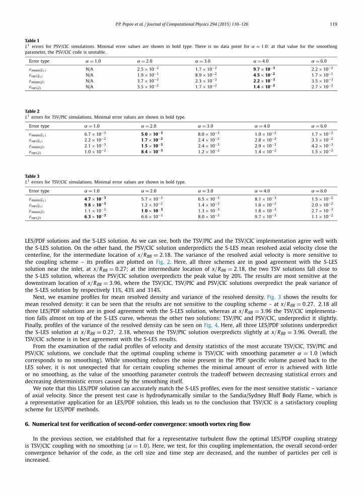
The errors for var (u1) , mean (ρ) and var (ρ), respectively εvar(u1), εmean(ρ) and εvar(ρ) , are analogously defined. Tables 1, 2, and 3 present the values for εmean(u1), εvar(u1), εmean(ρ) and εvar(ρ) for all simulation cases. Based on these results, we conclude that for PSV/CIC, the optimal choice for smoothing parameter is α = 4.0, for TSV/PIC it is α = 2.0, and for TSV/CIC it is α = 1.0.

Next, we compare the three solutions with optimal smoothing parameter values for the respective coupling scheme, in order to arrive at the optimal coupling scheme overall. Radial profiles of the statistics are examined at three axial locations: at x/RBB = 0.27, 2.18 and 3.96. Fig. 1 presents a comparison between the mean resolved axial velocity profiles of the three


Table 1L1 errors for PSV/CIC simulations. Minimal error values are shown in bold type. There is no data point for α = 1.0: at that value for the smoothing parameter, the PSV/CIC code is unstable.

Error type α = 1.0 α = 2.0 α = 3.0 α = 4.0 α = 6.0

εmean(u1) N/A 2.5 × 10−2 1.7 × 10−2 9.7 × 10−3 2.2 × 10−2

εvar(u1) N/A 1.9 × 10−1 8.9 × 10−2 4.5 × 10−2 1.7 × 10−1

εmean(ρ) N/A 3.7 × 10−3 2.3 × 10−3 2.2 × 10−3 3.5 × 10−3

εvar(ρ) N/A 3.5 × 10−2 1.7 × 10−2 1.4 × 10−2 2.7 × 10−2

Table 2L1 errors for TSV/PIC simulations. Minimal error values are shown in bold type.

Error type α = 1.0 α = 2.0 α = 3.0 α = 4.0 α = 6.0

εmean(u1) 6.7 × 10−3 5.0 × 10−3 8.0 × 10−3 1.0 × 10−2 1.7 × 10−2

εvar(u1) 2.2 × 10−2 1.7 × 10−2 2.4 × 10−2 2.8 × 10−2 3.3 × 10−2

εmean(ρ) 2.1 × 10−3 1.5 × 10−3 2.4 × 10−3 2.9 × 10−3 4.2 × 10−3

εvar(ρ) 1.0 × 10−2 8.4 × 10−3 1.2 × 10−2 1.4 × 10−2 1.5 × 10−2

Table 3L1 errors for TSV/CIC simulations. Minimal error values are shown in bold type.

Error type α = 1.0 α = 2.0 α = 3.0 α = 4.0 α = 6.0

εmean(u1) 4.7 × 10−3 5.7 × 10−3 6.5 × 10−3 8.1 × 10−3 1.5 × 10−2

εvar(u1) 9.8 × 10−3 1.2 × 10−2 1.4 × 10−2 1.6 × 10−2 2.0 × 10−2

εmean(ρ) 1.1 × 10−3 1.0 × 10−3 1.3 × 10−3 1.8 × 10−3 2.7 × 10−3

εvar(ρ) 6.3 × 10−3 6.6 × 10−3 8.0 × 10−3 9.7 × 10−3 1.1 × 10−2

LES/PDF solutions and the S-LES solution. As we can see, both the TSV/PIC and the TSV/CIC implementation agree well with the S-LES solution. On the other hand, the PSV/CIC solution underpredicts the S-LES mean resolved axial velocity close the centerline, for the intermediate location of x/RBB = 2.18. The variance of the resolved axial velocity is more sensitive to the coupling scheme – its profiles are plotted on Fig. 2. Here, all three schemes are in good agreement with the S-LES solution near the inlet, at x/RBB = 0.27; at the intermediate location of x/RBB = 2.18, the two TSV solutions fall close to the S-LES solution, whereas the PSV/CIC solution overpredicts the peak value by 20%. The results are most sensitive at the downstream location of x/RBB = 3.96, where the TSV/CIC, TSV/PIC and PSV/CIC solutions overpredict the peak variance of the S-LES solution by respectively 11%, 43% and 314%.

Next, we examine profiles for mean resolved density and variance of the resolved density. Fig. 3 shows the results for mean resolved density: it can be seen that the results are not sensitive to the coupling scheme – at x/RBB = 0.27, 2.18 all three LES/PDF solutions are in good agreement with the S-LES solution, whereas at x/RBB = 3.96 the TSV/CIC implementa-tion falls almost on top of the S-LES curve, whereas the other two solutions: TSV/PIC and PSV/CIC, underpredict it slightly. Finally, profiles of the variance of the resolved density can be seen on Fig. 4. Here, all three LES/PDF solutions underpredict the S-LES solution at x/RBB = 0.27, 2.18, whereas the TSV/PIC solution overpredicts slightly at x/RBB = 3.96. Overall, the TSV/CIC scheme is in best agreement with the S-LES results.

From the examination of the radial profiles of velocity and density statistics of the most accurate TSV/CIC, TSV/PIC and PSV/CIC solutions, we conclude that the optimal coupling scheme is TSV/CIC with smoothing parameter α = 1.0 (which corresponds to no smoothing). While smoothing reduces the noise present in the PDF specific volume passed back to the LES solver, it is not unexpected that for certain coupling schemes the minimal amount of error is achieved with little or no smoothing, as the value of the smoothing parameter controls the tradeoff between decreasing statistical errors and decreasing deterministic errors caused by the smoothing itself.

We note that this LES/PDF solution can accurately match the S-LES profiles, even for the most sensitive statistic – variance of axial velocity. Since the present test case is hydrodynamically similar to the Sandia/Sydney Bluff Body Flame, which is a representative application for an LES/PDF solution, this leads us to the conclusion that TSV/CIC is a satisfactory coupling scheme for LES/PDF methods.

6. Numerical test for verification of second-order convergence: smooth vortex ring flow

In the previous section, we established that for a representative turbulent flow the optimal LES/PDF coupling strategy is TSV/CIC coupling with no smoothing (α = 1.0). Here, we test, for this coupling implementation, the overall second-order convergence behavior of the code, as the cell size and time step are decreased, and the number of particles per cell is increased.


Fig. 1. Comparison of the radial profiles of the mean of the resolved axial velocity yielded by the LES/PDF coupling schemes with optimal values for the smoothing parameter α.

The computational domain is a cylinder of axial length 2.0 m and radius 1.5 m. Using χE (q) to denote the indicator function of q ∈ E , for a given set E , the initial velocity field is axi-symmetric, analytically specified as a superposition of a vortex ring and a jet (the following equations are in MKS units, which are omitted in order to avoid clutter):

ρux (x, r, t = 0) = 0.5 × e−r2/4 − χ1sin2 (2π (q1 − 0.05)) × ((r − 0.65)/(rq1)) , (29)

ρur (x, r, t = 0) = χ1sin2 (2π (q1 − 0.05)) × ((x − 0.65)/(rq1)) , (30)

ρuθ (x, r, t = 0) = 0, (31)

q1 =((x − 0.65)2 + (r − 0.65)2

)1/2, (32)

χ1 = χ[0.05,0.55] (q1) . (33)

Similarly, the initial condition for the mixture fraction mean and variance has the following analytic form:

ξ (x, r, t = 0) = 0.1 + 0.8 × χ2cos2 (πq2) , (34)

q2 =((x − 0.65)2 + (max(r − 0.5,0) × 3/5)2

)1/2, (35)

χ2 = χ[0,0.5] (q2) , (36)

ξ ′′ (x, r, t = 0) = 0.5ξ(1 − ξ

). (37)


Fig. 2. Comparison of the radial profiles of the variance of the resolved axial velocity yielded by the LES/PDF coupling schemes with optimal values for the smoothing parameter α.

The material property definitions are analogous to the previous test case, with the exception that the molecular viscosity and diffusivity, ν and D , have been scaled by a constant (ν0 = 1.5 × 10−3

[m2

s

]in Eq. (10)) in order to yield a value for

the Reynolds number of Re = 3000, based on the cylinder’s radius and the maximal velocity in the initial condition. For turbulence modeling we use a large filter of fixed size = 0.5m, instead of the traditional dynamic Smagorinsky procedure. This yields a grid-independent solution, which is necessary in order to test the overall order of convergence of the LES/PDF code.

The order of convergence is tested by taking the differences between the final values of u1, ξ, ξ2, and ρ , as obtained by the LES/PDF simulation, and a highly resolved S-LES solution on a 128 × 128 × 64 grid. These differences are averaged over the azimuthal direction, integrated against a collection of 16 Fourier modes in x–r space, and the overall error is defined as the root-mean-square error of these 16 functionals.

More concretely, for measuring error based on the resolved axial velocity, we define the functionals g j,k by

g j,k =∫

x∈[0,2],r∈[0,1.5]u1 (x, r, θ) eiπ(2 jx+1.5kr)rdrdxdθ, (38)

and then we define the error measure for resolved axial velocity, εu1 , as

εu1 =⎛⎝ 4∑

j,k=1

∣∣∣E (gLES/PDFj,k − gS-LES

j,k

)∣∣∣2⎞⎠1/2

, (39)

where we use E (·) to denote the expectation of a random variable. An error measure based on the functionals used in Eq. (38) is chosen because the evaluation of these linear functionals of the LES/PDF solution contains no bias error, and


Fig. 3. Comparison of the radial profiles of the mean of the resolved density yielded by the LES/PDF coupling schemes with optimal values for the smoothing parameter α.

therefore the error measure itself is more accurate than if something line an L2 norm were used in Eq. (38). The error mea-sures for resolved mixture fraction, resolved square mixture fraction, and resolved density, εξ , εξ2 and ερ respectively, are similarly defined. Convergence of the LES/PDF algorithm with respect to these error measures verifies the weak convergence properties of the method. In the present context, weak convergence is taken to mean convergence of the expectations of general linear functionals of the end solution, as opposed to standard pointwise convergence.

Convergence studies of LES/PDF computational algorithms, such as the one we present here, are rare [5,6], due to the high cost introduced by the stochastic nature of the PDF aspect of the code. In particular, for a grid with a cell size of x, a time step of length t , Npc particles per cell and Np particles total, and a fixed value of the smoothing parameter α[6], second-order convergence of the overall code with respect to the grid size and time step implies that the errors in the functionals g j,k scale in the following manner:

ε = C1x2 + C2t2 + C31

Npc+ C4

(1

Np

)1/2

Y . (40)

In the above equation, the four terms on the right represent, respectively, errors due to grid resolution, time step, statistical bias and statistical errors, where Y is a Gaussian random variable of zero mean and unit variance. The last component in the above expression, which is due to statistical error, illustrates the advantage of using error norms based on linear functional

of the solution, as opposed to pointwise error estimates: for the latter, the statistical error scales as (

1N pc

)1/2, which is

much larger than (

1N p

)1/2.

Even for the linear functionals considered above, the bias error scales as 1N pc

. The scaling of the bias error implies that, in order to test second-order convergence with respect to the grid and time step, we need to increase the number of particles


Fig. 4. Comparison of the radial profiles of the variance of the resolved density yielded by the LES/PDF coupling schemes with optimal values for the smoothing parameter α.

per cell by a factor of 4 each time that x and t are decreased by a factor of 2, and hence the overall number of particles is increased by a factor of 32.

We perform simulations on five successively more refined grids. The simulation parameters are summarized in the table below. The overall computational cost is also provided

Simulation type Grid size (nx × nr × nθ ) Particles per cell (Npc ) Time step, t Cost (CPU hours)

S1 16 × 16 × 8 20 0.0160 3.3 × 10−3

S2 24 × 24 × 8 35 0.0106 2.0 × 10−2

S3 32 × 32 × 16 50 0.0080 0.14S4 48 × 48 × 16 112 0.0066 0.88S5 64 × 64 × 32 200 0.0040 9.83

In the above table, note that, for Npc to be proportional to x−2, Npc for S1 would have to be 12 (or 13), and Npc for S2would have to be 28. The higher numbers of Npc = 20 for S1 and Npc = 35 for S2 are used in order to ensure a stable run of the particle PDF code. For the simulations S3, S4, S5, on whose data points the second-order convergence is primarily based, the relationship Npc ∝ x−2 is maintained. Contours of the resolved axial velocity and resolved mixture fraction at the end time, t = 0.45, are shown on Fig. 5.


Fig. 5. Resolved axial velocity (top) and resolved mixture fraction (bottom) fields at the end time, t = 0.45 of the smooth vortex ring test case. From left to right, results are shown for the simulations S1, S3, S5 and the S-LES simulation.

For each of the simulation types S1 through S5, we perform, for the purpose of estimating confidence intervals for g j,k , 8 independent simulations, with different initial seeds for the random number generator. The 95% confidence interval width for the error measures εu1 , εξ , εξ2 , ερ is estimated by the formula:

CI width = 1.96 ×

√√√√√1

8

4∑j,k=1

Var(

g j,k). (41)

The computed error from these simulations can be seen on Fig. 6, which plots, on a log–log scale, the means and confidence intervals for εu1 , εξ , εξ2 , ερ against x, the grid cell size in the axial direction. Since t is directly proportional to x for S1 through S5, second order convergence with respect to the grid and time step corresponds to the data points falling on a straight line of slope 2 in this log–log plot.

As can be seen on Fig. 6, all four error measures indicate second-order convergence – the reference line of slope 2 passes through the confidence intervals of the S3, S4, S5 data points, and with the exception of the S1 data points for ε

ξ2 and εu1 , the errors for the coarse-grid S1 and S2 simulation types are also close to the reference line of slope 2. From these results, we conclude that the LES/PDF scheme implemented in this work is indeed second-order accurate with respect to the grid size and time step.

7. Conclusions

In this paper, we have addressed the issue of coupling between the LES and PDF components of an LES/PDF algorithm for turbulent combustion simulations. A coupling methodology has been proposed which allows for second-order overall accuracy of the algorithm with respect to the grid cell size and the time step. Using a numerical test case based on the


Fig. 6. Mean errors and 95% confidence intervals for the convergence simulations S1 through S5. The grey and black reference lines indicate respectively first and second-order convergence behavior.

turbulent Sandia/Sydney Bluff Body Flame, it has been determined that the optimal coupling scheme is that which uses the auxiliary transported specific volume approach with cloud in cell mean estimation and no smoothing. Finally, for this choice of coupling scheme, convergence studies have been performed to verify the second-order accuracy of the LES/PDF algorithm.

Acknowledgements

This work is supported in part by the Air Force Office of Scientific Research, Grant FA 9550-09-1-0047, and by NASA Grant NNX08A B 36A.

References

[1] S.B. Pope, PDF methods for turbulent reactive flows, Prog. Energy Combust. Sci. 11 (1985) 119–192.[2] S.B. Pope, Turbulent Flows, Cambridge University Press, Cambridge, 2000.[3] D.C. Haworth, Progress in probability density function methods for turbulent reacting flows, Prog. Energy Combust. Sci. 36 (2) (2010) 168–259.[4] Y.Z. Zhang, D.C. Haworth, A general mass consistency algorithm for hybrid particle/finite volume PDF methods, J. Comput. Phys. 194 (2004) 156–193.[5] H. Wang, P.P. Popov, S.B. Pope, Weak second-order splitting schemes for Lagrangian Monte Carlo particle methods for the composition PDF/FDF trans-

port equations, J. Comput. Phys. 229 (2010) 1852–1878.[6] S. Viswanathan, H. Wang, S.B. Pope, Numerical implementation of mixing and molecular transport in LES/PDF studies of turbulent reacting flows,

J. Comput. Phys. 230 (2011) 6916–6957.[7] C.D. Pierce, P. Moin, Progress-variable approach for large-eddy simulation of turbulent combustion, J. Fluid Mech. 504 (2004) 73–97.[8] V.A. Sabel’nikov, O. Soulard, Rapidly decorrelating velocity-field model as a tool for solving one-point Fokker–Planck equations for probability density

functions of turbulent reactive scalars, Phys. Rev. E 72 (2005).[9] P. Colucci, F. Jaberi, P. Givi, S.B. Pope, Filtered density function for large eddy simulation of turbulent reacting flows, Phys. Fluids 10 (1998) 499–515.

[10] F. Jaberi, P. Colucci, S. James, P. Givi, S.B. Pope, Filtered mass density function for large eddy simulation of turbulent reacting flows, J. Fluid Mech. 401 (1999) 85–121.

[11] V. Raman, H. Pitsch, A consistent LES/Filtered density function formulation for the simulation of turbulent flames with detailed chemistry, Proc. Combust. Inst. 31 (2007) 1711–1719.

[12] Y. Ge, M.J. Cleary, A.Y. Klimenko, Sparse-Lagrangian FDF simulations of Sandia Flame E with density coupling, Proc. Combust. Inst. 33 (2011).[13] M. Muradoglu, P. Jenny, S.B. Pope, D.A. Caughey, A consistent hybrid finite-volume/particle method for the PDF equations of turbulent reactive flows,

J. Comput. Phys. 154 (1999) 342–371.[14] A.R. Masri, R.W. Bilger, Turbulent diffusion flames of hydrocarbon fuels stabilized on a bluff body, Proc. Combust. Inst. 20 (1985) 319–326.[15] P.E. Kloeden, E. Platen, Numerical Solution of Stochastic Differential Equations, Springer-Verlag, Berlin, 1992.[16] S.B. Pope, Computations of turbulent combustion: progress and challenges, Proc. Combust. Inst. 23 (1991) 591–612.[17] H. Pitsch, Large-eddy simulation of turbulent combustion, Annu. Rev. Fluid Mech. 38 (2006) 453–482.

http://refhub.elsevier.com/S0021-9991(15)00120-5/bib31s1
























[18] H. Wang, S.B. Pope, Large eddy simulation/probability density function modeling of a turbulent CH4/H2/N2 jet flame, Proc. Combust. Inst. 33 (2011) 1319–1330.

[19] K.A. Kemenov, H. Wang, S.B. Pope, Turbulence resolution scale dependence in large-eddy simulations of a jet flame, Flow Turbul. Combust. 88 (4) (2012) 529–561, http://dx.doi.org/10.1007/s10494-011-9380-x.

[20] R. Mustata, L. Valino, C. Jimenez, W.P. Jones, S. Bondi, A probability density function Eulerian Monte Carlo field method for large eddy simulations: applications to a turbulent piloted methane/air diffusion flame (Sandia D), Combust. Flame 145 (2006) 88–104.

[21] L. Valiño, A field Monte Carlo formulation for calculating the probability density function of a single scalar in a turbulent flow, Flow Turbul. Combust. 60 (1998) 157–172.

[22] S.B. Pope, A Monte Carlo method for the PDF equations of turbulent reactive flow, Combust. Sci. Technol. 25 (1981) 159–174.[23] P.P. Popov, S.B. Pope, Large eddy simulation/probability density function simulations of bluff body stabilized flames, Combust. Flame 161 (2014)

3100–3133.[24] R.O. Fox, Computational Methods for Turbulent Reacting Flows, Cambridge University Press, Cambridge, 2003.



http://dx.doi.org/10.1007/s10494-011-9380-x









journal of computational physics - cornell university of computational physics 294 (2015) 110–126...

Documents