lecture 7 to 16 - imperial college london · imperial college [email protected] lecture...

EE1 and EIE1: Introduction to Signals and Communications

Professor Kin K. Leung

EEE and Computing Departments

Imperial College

[email protected]

Lecture seven

2

Lecture Aims

● To introduce linear systems

● To introduce convolution

● To give examples of real and ideal filters

Linear Systems

3

Linear Time Invariant System

h(t) g(t) y(t)

Linear Systems (continued)

● A system converts an input signal g(t) in an output signal y(t).

● Assume the output for an input signal g1(t) is y1(t) and the output for an input g2(t) is y2(t). The system is linear if the output for input g1(t) + g2(t) is y1(t)+ y2(t).

● A system is time invariant if its properties do not change with the time. That is, if the response to g(t) is y(t), then the response to g(t - t0) is going to be y(t -t0)

4

Linear

Systemg(t) y(t)

Linear

Systemg1(t) + g2(t) y1(t) + y2(t)

Linear

Systemg(t-t0) y(t-t0)

Unit impulse response of a LTI system

Consider a linear time invariant (LTI) system. Assume the input signal is a Dirac function δ(t). Call the observed output h(t).

● h(t) is called the unit impulse response function.

● With h(t), we can relate the input signal to its output signal through the convolution formula:

5

y(t) h(t) * g(t) h( )g(t )d .

Physical interpretation of linear system response

δ(t)

t0

6

Input Output

δ(t-to)

t0 to t0

???

t0

h(t) : unit-impulse response


δ(t)

t0

7

Input Output

δ(t-to)

t0 to t0 to

δ(t-to)

t0 to

δ(t)

t0

???

t0

h(t): unit-impulse response

h(t-to) Time invariant


δ(t)

t0

8

Input Output

δ(t-to)

t0 to t0 to

δ(t-to)

t0 to

δ(t)

t0

h(t)

h(t-to)

t0

h(t)+h(t-to)

to

Linearity


9

Input Output

b δ(t-to)

t0 to

a δ(t)

t0

a h(t)+b h(t-to)

to

Linearity

g(nΔτ)

…

Δτ

t0 t0

???

0 n

t

…

input g(nΔτ): output g(nΔτ)Δτ h(t-nΔτ)

g(t)

y(t) = ∑ g(nΔτ)Δτ h(t-nΔτ)

dthgtgthty )()()(*)()(

Intuitive explanation of the convolution formula

● g(t) can be approximated as g(t) ≅ Σng(n∆τ)∆τδ(t−n∆τ).

● In the limit as ∆τ→0 this approximation approaches the true function g(t).

● The response ŷ(t) of the LTI system to the input asΣng(n∆τ)∆τδ(t−n∆τ) is going to be Σng(n∆τ)h(t−n∆τ)∆τ .

● Thus, y(t) = lim∆→0Σng(n∆τ)h(t−n∆τ)∆τ=

10

g()h(t )d .

Graphical Interpretation of Convolution (1)

u

duutguftgtf )()()(*)(

t

g(t)

0t

f(t)

0 b-a

11


u


u

g(-u)

0u

g(u)

0

u

g(t-u)

0

t<0

u

g(t-u)

0

t>0

u

f(u)

0 b-aa, b: positive

12

right shift by tleft shift by t


u


g(t-u)

-<t<-a

u

f(u)

0 b-a

g(t-u)

t>b

u

f(u)

0 b-a

g(t-u)

-a<t<b

u

f(u)

0 b-a

Depending on t, the convolution

integral is the area under f(u)g(t-u).

Search “Convolution” on the Wikipedia

site for an animation of convolution.13

Convolution in the frequency domain

The convolution of two functions g(t) and h(t), denoted by g(t) ∗ h(t), is defined by the integral

If g(t) ⇔ G(ω) and h(t) ⇔ H(ω) then the convolution reduces to a product in the Fourier domain

H(ω) is called the system transfer function or the system frequency response or the spectral response.

Notice that, for symmetry, a product in the time domain corresponds to a convolution in frequency domain. That is

14

( ) ( )* ( ) ( ) ( ) .y t h t g t h x g t x dx

( ) ( )* ( ) ( ) ( ) ( ).y t h t g t Y w H G

1 2 1 2

1( ) ( ) ( )* ( ).

2g t g t G G

Bandwidth of the product of two signals

If g1(t) and g2(t) have bandwidths B1 and B2 Hz, respectively.

The bandwidth of g1(t) g2(t) is B1 + B2 Hz.

15

Ideal Low-Pass Filter

Ideal low-pass filter response

Ideal low-pass filter impulse response

16

h(t) W

sinc W t t

d

H () rect 2W e j td

Ideal High-Pass and Band-pass filters

17

Figure 1: Ideal high-pass filter Figure 2: Ideal band-pass filter

Practical filters

● The filters in the previous examples are ideal filters.

● They are not realizable since their unit impulse responses are everlasting (Think of the sinc function).

● Physically realizable filter impulse response h(t) = 0 for t < 0.

● Therefore, we can only obtain approximated version of the ideal low-pass, high-pass and band-pass filters.

18

Example of a linear system: RC circuit

19

Example: RC circuit (continued)

and

Therefore, this circuit behaves as a low-pass filter.

20

1 1

( )1 1

1

j C aH

R j C j RC a j

aRC

2 2

1

( ) (0) 1, lim ( ) 0.

tan

w

h

aH H H

a

a

Summary

● Linear time invariant systems

● Unit impulse response function

● Convolution formula:

● Low-pass, high-pass and band-pass filters

21

( ) ( )* ( ) ( ) ( )y t h t g t h g t d




Imperial College

[email protected]

Lecture eight

23

Lecture Aims

● To introduce Energy spectral density (ESD)

● Input and Output Energy spectral densities

● To introduce Power spectral density (PSD)

● Input and Output Power spectral densities

Signal Energy, Parseval’s Theorem

Consider an energy signal g(t), Parseval’s Theorem states that

Proof:

24

Eg g(t)

2dt

t

1

2G()

2d

2

1( ) *( ) ( ) *( )

2

1 *( ) ( )

21 1

( ) *( ) ( )2 2

j tg

j t

E g t g t dt g t G e d dt

G g t e dt d

G G d G d

Example

Consider the signal g(t) = e-atu(t) (a > 0)

Its energy is

We now determine Eg using the signal spectrum G() given by

It follows

which verifies Parseval’s theorem.

25

2 2

0

1( )

2at

gE g t dt e dta

1( )G

j a

2 12 2

1 1 1 1 1( ) tan

2 2 2 2gE G d da a a a

Energy Spectral Density

● Parseval’s theorem can be interpreted to mean that the energy of a signal g(t)is the result of energies contributed by all spectral components of a signal g(t)

● The contribution of a spectral component of frequency is proportional to |G()|2

● Therefore, we can interpret |G()|2 as the energy per unit bandwidth of the spectral components of g(t) centered at frequency

● In other words, |G()|2 is the energy spectral density of g(t)

26

Energy Spectral Density (continued)

The energy spectral density (ESD) is thus defined as

and

Thus, the ESD of the signal g(t) = e-atu(t) of the previous example is

27

2( ) ( )G

Eg 1

2()d

2

2 2

1( ) ( )G

a

( )

Energy of modulated signals (important)

Let g(t) be a baseband energy signal with energy Eg.

The energy of the modulated signal φ(t) = g(t)cos0t is half the energy of g(t). That is,

Proof: Go from the definition of energy being the integration of the magnitude squared of the signal over the whole time horizon. (0 is assumed to be equal to or larger than 2π times the bandwidth of g(t).)

The same applies to power signals. That is, if g(t) is a power signal then

(You will use this result when computing the efficiency of a Full AM system).

28

1.

2 gE E

1.

2 gP P

Time Autocorrelation Function and ESD

For a real signal the autocorrelation function is defined as

Do you remember the correlation of two signals (lecture three)? The autocorrelation function measure the correlation between g(t) and all its translated versions.

Notice

and

But, most important...

29

( ) ( ) ( )g g t g t dt

( ) ( ).g g

( )* ( ) ( ).gg g

( )g

Time Autocorrelation Function and ESD

...the Fourier transform of the autocorrelation function is the Energy Spectral Density! That is

Proof:

The Fourier transform of g(τ+t) is G(ω) ejωt . Therefore,

30

2( ) ( ) ( )g G

( ) ( ) ( )

( ) ( )

jg

j

F e g t g t dt d

g t g t e d dt

2( ) ( ) ( ) ( ) ( ) ( )j t

gF G g t e dt G G G

ESD of the Input and the Output

If g(t) and y(t) are the input and the corresponding output of a LTI system, then

Therefore,

This shows that

Thus, the output signal ESD is |H(ω)|2 times the input signal ESD.

31

Y () H()G().

2 2 2( ) ( ) ( ) .Y H G

2( ) ( ) ( ).y gH

Signal Power and Power Spectral Density

The power Pg of a real signal g(t) is given by

All the results for energy signals can be extended to power signals. Call Sg(ω) the Power Spectral Density (PSD) of g(t). Thus,

Sg(ω) can be found using the autocorrelation function.

32

2 2

2

1lim ( ) .

T

g TTP g t dt

T

1( ) .

2g gP S d

Time autocorrelation Function of Power Signals

The (time) autocorrelation function of a real deterministic power signal g(t) is defined as

We have that

If g(t) and y(t) are the input and the corresponding output of a LTI system, then

Thus, the output signal PSD is |H(ω)|2 times the input signal PSD.

33

2

2

1( ) lim ( ) ( )

T

g TTR g t g t dt

T

Rg () Sg ()

2( ) ( ) ( ).y gS H S

( )gR

Relationships among these signals and functions

Output PSD is |H(ω)|2 times

the input signal PSD.

34

2

2

1( ) lim ( ) ( )

T

g TTR g t g t dt

T

Rg( ) S

g()

Tlim 1

T|G() |2

)()( Gtg

Input

LTI system

)()( Hth

)()()(*)()( GHtgthty

)()( yy SR

Sy()

Tlim 1

T| H () |2|G() |2

| H () |2 Sg()

Output

Conclusions

We learned about

● Energy and Power Spectral Densities

● Time autocorrelation functions

● Input and output energies and powers

35




Imperial College

[email protected]

Lecture nine

37

Lecture Aims

● To examine modulation process

● Baseband and bandpass signals

● Double Sideband Suppressed Carrier (DSB-SC)- Modulation

- Demodulation

● Modulators- Nonlinear modulators

- Switching modulators

- Diode modulators

Modulation

● Modulation is a process that causes a shift in the range of frequencies in a signal.

● Two types of communication systems

- Baseband communication: communication that does not use modulation

- Carrier modulation: communication that uses modulation

● The baseband is used to designate the band of frequencies of the source signal. (e.g., audio signal 4kHz, video 4.3MHz)

38

Modulation (continued)

In analog modulation the basic parameter such as amplitude, frequency or phase of a sinusoidal carrier is varied in proportion to the baseband signal m(t). This results in amplitude modulation (AM) or frequency modulation (FM) or phase modulation (PM).

The baseband signal m(t) is the modulating signal.

The sinusoid is the carrier or modulator.

39

Why modulation?

● To use a range of frequencies more suited to the medium

● To allow a number of signals to be transmitted simultaneously (frequency division multiplexing)

● To reduce the size of antennas in wireless links

40

Amplitude Modulation

● Carrier

- Phase is constant

- Frequency is constant

● Modulating signal

● With amplitude spectrum

41

cos( )c cA t c 0

m(t)

Modulated signal

● Modulated signal:

42

m(t)cosct

Modulated signal


43

m(t)cosct

Modulated signal

● Baseband spectrum:

● M() is shifted to M(+ c) and M(- c)

44

B Hz

Demodulation of DSB signal

● Process modulated signal

● Multiply modulated signal with

45

m(t)cosct

cosct

2 1( ) ( ) cos ( ) ( ) cos 2

21 1

( ) ( ) ( 2 ) ( 2 )2 4

c c

c c

e t m t t m t m t t

E M M M



46

m(t)cosct

Example

● Modulating signal m(t)=cos mt

● Carrier cos ct

● Modulated signal ϕ(t) = m(t) cos ct =cos mt cos ct

47

Amplitude spectrum

● Baseband signal

48

1( ) cos( ) cos( )

2DSB SC c m c mt t t

( ) ( ) ( )m mM

(c

m)



49

m(t)cosct

Modulators

● We need to implement multiplication m(t) cos ct

● We can use

- Nonlinear modulators

- Switching modulators

● Switching modulators can be implemented using diode ring modulators

50

Nonlinear modulator

● Input-output characteristics of a nonlinear element

● Where x(t) is the input signal and y(t) is the output signal

● Consider to input signals

51

2( ) ( ) ( )y t ax t bx t

1

2

( ) cos ( )

( ) cos ( )c

c

x t t m t

x t t m t

Nonlinear modulator

● Let us implement

52

1 2

2 21 1 2 2

( ) ( ) ( )

( ) ( ) ( ) ( )

z t y t y t

ax t bx t ax t bx t

( ) 2 ( ) 4 ( )cos cz t am t bm t t

Switching modulator

● Consider a periodic signal of fundamental frequency c

● Multiplication of modulating signal with this periodic signal gives

● The spectrum of the product m(t)ϕ(t) is the spectrum M() shifted to

53

0

( ) cos( )n c nn

t C n t

0

( ) ( ) ( ) cos( )n c nn

m t t C m t n t

, 2 , , , c c cn

Square Pulse train as a modulator

● Consider a square pulse train

● The Fourier series for this periodic waveform is

● The signal m(t)w(t) is

54

1 2 1 1( ) cos cos3 cos5

2 3 5c c cw t t t t

1 2 1( ) ( ) ( ) ( ) cos ( ) cos3

2 3c cm t w t m t m t t m t t

Switching modulator

55

Diode Switches

56

Ring modulator

57

Ring modulator

58

0

4 1 1( ) cos cos3 cos5

3 5c c cw t t t t

0

4 1 1( ) ( ) ( ) ( ) cos ( )cos3 ( )cos5

3 5i c c cv t m t w t m t t m t t m t t

Conclusions

We learned about

● Baseband and Carrier transmission

● Amplitude modulation (DSB-SC)

● Non-linear modulator

● Switching modulator

● Diode switches

59

EE1 and ISE1: Introduction to Signals and Communications



Imperial College

[email protected]

Lecture ten

61

Lecture Aims

● To examine full AM process

● AM signal and its envelope

● Sideband carrier power

● Generation of AM signals

● Demodulation of AM signals

Double Sideband Suppressed Carrier

● A receiver must generate a carrier in frequency and phase synchronism with the carrier at the transmitter

● This calls for sophisticated receiver and could be quite costly

● An alternative is for the transmitter to transmit the carrier along with the modulated signal

● In this case the transmitter needs to transmit much larger power

62

Amplitude Modulation

● Carrier

- Phase is constant

- Frequency is constant.

● Modulation signal

● With amplitude spectrum

● Full AM signal is

● Spectrum of full AM signal

63

A cos(ct c )c 0

m(t)

( ) cos ( ) cos

( ) cosAM c c

c

t A t m t t

A m t t

1( ) ( ) ( ) ( ) ( )

2AM c c c ct M M A

Full AM Modulated signal

● DSB Modulated signal:

● Full AM signal

64

Full AM Modulated signal

● Signal



65

( ) cos cA m t t

Envelope detection is not possible when

● Signal



66

( ) cos cA m t t

Envelope detection condition

● Detection condition A + m(t) ≥ 0

● Let mp be the maximum negative value of m(t). This means that m(t) ≥ -mp

● When we have A ≥ mp, we can use envelope detector

● The parameter is called the modulation index

● When 0 ≤ μ ≤ 1, we can use an envelope detector

67

pm

A

Envelope detection example


● Modulating signal amplitude is

● Hence and

● Modulating and modulated signals are

68

( ) cos mm t B t

pm B

B

A B A

( ) cos cos

( ) ( ) cos 1 cos cosm m

AM c m c

m t B t A t

t A m t t A t t


● Consider modulation index to be

● For modulation index

69

0.5

1

Sideband and Carrier power

● Consider full AM signal

● Power Pc of the carrier A cos ct

● Power Ps of the sideband signals

● Power efficiency

70

carrier sidebands

( ) cos ( )cosAM c ct A t m t t

2 2A

20.5 ( )m t

2

2 2

useful power ( )100%

total power ( )s

c s

P m t

P P A m t

Maximum power efficiency of Full AM

● When we have

● Signal power is

● When 0 ≤ μ ≤ 1

● When modulation index is unity, the efficiency is

● When μ=0.3 the efficiency is

71

( ) cos mm t A t

22 ( )( )

2

Am t

max 33%

2

2

0.3100% 4.3%

2 0.3

Generation of AM signals

● Full AM signals can be generated using DSB-SC modulators

● But we do not need to suppress the carrier at the output of the modulator, hence we do not need a balanced modulators

● Use a simple diode

72

Simple diode modulator design

● Input signal

● Consider the case c >> m(t)

● Switching action of the diode is controlled by

● A switching waveform

is generated. The diode open and shorts periodically with w(t)

● The signal is generated

73

cos ( )cc t m t

cos cc t

' ( ) cos ( ) ( )bb cv t c t m t w t

Diode Modulator

● Diode acts as a multiplier

74

n

suppressed byAM bandpass filter

( ) cos ( ) ( )

1 2 1 1 cos ( ) cos cos3 cos5

2 3 5

2 cos ( )cos other terms

2

bb c

c c c c

c c

v t c t m t w t

c t m t t t t

ct m t t

Demodulation of AM signals

● Rectifier detector

75

Demodulation of AM signals

● Half-wave rectified signal is given by

where w(t)

76

R

( ) cos ( )R cA m t t w t

1 2 1 1( ) cos cos cos3 cos5

2 3 5

1 ( ) other terms of higher frequencies

R c c c cv A m t t t t t

A m t

Demodulation of AM signals using an envelope detector

77

● Simple detector

● Detector operation

Envelope detector example

● For the single tone

● Design envelope detector

78

Conclusions

● Examined full AM

● Sideband and carrier powers

● AM modulators

● AM demodulators

79




Imperial College

[email protected]

Lecture eleven

81

Lecture Aims

● To examine Single Sideband Modulation (SSB)

- Time domain representation

- Tone modulation

- Generation of SSB signals

- Demodulation of SSB signals

Modulation of Baseband Signals

Modulated Signal

82

Modulation of Baseband Signals

Splitting the baseband spectrum into USB and LSB

83

Single Sideband Generation

84

Time-Domain Representation of SSB signals

● Let m+(t) and m−(t) be the inverse Fourier transforms of M+(ω) and M−(ω).

● Because the amplitude spectra |M+(ω)| and |M−(ω)| are not even functions of ω, the signals m+(t) and m−(t) cannot be real. They are complex.

● It can be proven that m+(t) and m−(t) are conjugates. Moreover, m+(t) + m−(t)= m(t). Hence,

85

1( ) ( ) ( )

21

( ) ( ) ( )2

h

h

m t m t jm t

m t m t jm t

Time-Domain Representation of SSB signals

To determine mh(t) note that

Since , it follows . Hence

. But . Therefore

The right-hand side of this last equation defines the Hilbert transform of m(t).

86

( ) ( ) ( )

1 ( ) 1 sgn( )

21 1

( ) ( )sgn( )2 2

M M u

M

M M

1( ) ( ) ( )

2 hm t m t jm t ( ) ( )sgn( )hjm t M

( ) ( )sgn( )hM jM 1 sgn( )t j

1 ( )( ) ( ) 1 .h

mm t m t t d

t

Hilbert Transform

The Hilbert Transform mh(t) is generated by passing m(t) through a filter h(t) with the following transfer function:

That is, and , for

87

2

2

0( ) sgn( )

0

j

j

j eH j

j e

( ) 1H ( ) 2h 0

Time-Domain Representation of SSB Signals

We can now express the SSB signal in terms of m(t) and mh(t).

Inverse transform gives

Using

88

( ) ( ) ( )USB c cM M

( ) ( ) ( )c cj t j tUSB t m t e m t e

1( ) ( ) ( )

21

( ) ( ) ( )2

h

h

m t m t jm t

m t m t jm t

( ) ( ) cos ( )sinUSB c h ct m t t m t t

Time-Domain Representation of SSB Signals

In a similar way we can show that

Hence a general SSB signal can be expressed as

where the minus sign applies to USB and the plus sign applies to LSB.

89

( ) ( ) cos ( )sin .LSB c h ct m t t m t t

( ) ( ) cos ( )sin ,SSB c h ct m t t m t t

SSB (t)

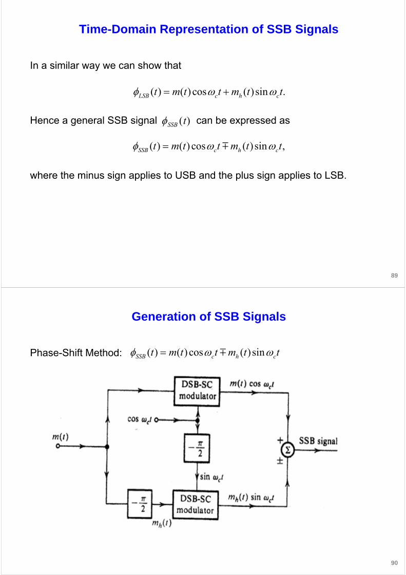
Generation of SSB Signals

Phase-Shift Method:

90

( ) ( ) cos ( )sinSSB c h ct m t t m t t

SSB Tone Modulation Example

● Consider single tone modulating signal:

● Hilbert transform requires phase shift by

● Delay in phase by yields

● Using , we get

91

( ) cos .mm t t

2.

2 ( ) cos( 2) sin .h m mm t t t


( ) cos cos sin sin cos( ) .SSB m c m c c mt t t t t t

SSB Tone Modulation Example

● Baseband spectrum

● USB spectrum

● LSB spectrum

92

Generation of SSB Signals

Selective-filtering method:

93

Coherent demodulation of SSB-SC signals

The SSB demodulator is identical to the synchronous demodulator used for DSB-SC.

Hence

Thus, the product yields the baseband signal and another SSB signal with carrier 2ωc. A low-pass filter will suppress the unwanted SSB terms.

94


1( )cos( ) ( ) 1 cos 2 ( )sin 2

21 1

( ) ( ) cos 2 ( )sin 22 2

SSB c c h c

c h c

t t m t t m t t

m t m t t m t t

( ) cos( )SSB ct

Conclusions

● Hilbert Transform

● Single Side Band (SSB) signals

● Modulation and demodulation of SSB signals

95




Imperial College

[email protected]

Lecture twelve

97

Lecture Aims

● Angle Modulation

- Phase and Frequency modulation

- Concept of instantaneous frequency

- Examples of phase and frequency modulation

- Power of angle-modulated signals

Angle modulation

Consider a modulating signal m(t) and a carrier vc(t) = A cos(ωct + θc).

The carrier has three parameters that could be modulated: the amplitude A (AM) the frequency ωc (FM) and the phase θc (PM).

The latter two methods are closely related since both modulate the argument of the cosine.

98

Instantaneous Frequency

● By definition a sinusoidal signal has a constant frequency and phase:

● Consider a generalized sinusoid with phase θ(t):

● We define the instantaneous frequency ωi as:

● Hence, the phase is

99

Acos(ct c )

(t) Acos(t)

( )i

dt

dt

( ) ( ) .t

it d

Phase modulation

We can transmit the information of m(t) by varying the angle θ of the carrier. In phase modulation (PM) the angle θ(t) is varied linearly with m(t) :

where kp is a constant and ωc is the carrier frequency. Therefore, the resulting PM wave is

The instantaneous frequency in this case is given by

100

( ) ( )c pt t k m t

( ) cos ( )PM c pt A t k m t

( ) ( )i c p

dt k m t

dt

Frequency modulation

In PM the instantaneous frequency ωi varies linearly with the derivative of m(t). In frequency modulation (FM), ωi is varied linearly with m(t). Thus

where kf is a constant. The angle θ(t) is now

The resulting FM wave is

101

( ) ( ).i c ft k m t

( ) ( ) ( ) .t t

c f c ft k m d t k m d

( ) cos ( )t

FM c ft A t k m d

Example

Sketch FM and PM signals if the modulating signal is the one above (on the left). The constants kf and kp are 2π×105 and 10π, respectively, and the carrier frequency fc

=100MHz.

102

FM example

● Instantaneous angular frequency

● Instantaneous frequency

103

( )i c fk m t

8 5( ) 10 10 ( )2

fi c

kf f m t m t

8 5min min

8 5max max

( ) 10 10 ( ) 99.9

( ) 10 10 ( ) 100.1

i

i

f m t MHz

f m t MHz

PM example


104

fi f

c

kp

2m(t) 108 5 m(t)

( fi)

min108 5 m(t) min

108 105 99.9MHz

( fi)

max108 5 m(t) max

108 105 100.1MHz

Power of an Angle-Modulated wave

● General angle modulated waveform

● Instantaneous phase and frequency vary with the time, but amplitude Aremains constant.

● Thus, the power of angle–modulated waves is always .

105

( ) cos ( )t A t

2

2

A

Conclusions

Examined


● PM and FM modulations

● Examples of PM and FM signals

106




Imperial College

[email protected]

Lecture thirteen

108

Lecture Aims

● To Study the bandwidth of angle modulated waves

- Narrow-Band Angle Modulation

- Carson’s rule

Bandwidth of Angle Modulated waves

In order to study bandwidth of FM waves, define

and

The frequency modulated signal is

109

( ) ( )t

a t m d

( ) ( )ˆ ( ) c f f cj t k a t jk a t j t

FM t Ae Ae e

ˆ( ) Re ( )FM FMt t

Bandwidth of Angle Modulated waves

Expanding the exponential in power series yields

and

110

e jk f a(t )

22ˆ ( ) 1 ( ) ( ) ( )

2! !c

nf f j tn n

FM f

k kt A jk a t a t j a t e

n

2 3

2 3

ˆ( ) Re ( )

cos ( )sin ( ) cos ( )sin2! 3!

FM FM

f fc f c c c

t t

k kA t k a t t a t t a t t

Narrow-Band Angle Modulation

The signal a(t) is the integral of m(t). It can be shown that if M(ω) is band limited to B, A(ω) is also band limited to B.

If |kf a(t)| ≪ 1 then all but the first term are negligible and

This case is called narrow-band FM.

Similarly, the narrow-band PM is given by

111

( ) ~ cos ( )sinFM c f ct A t k a t t

PM

(t) ~ A cosct k

pm(t)sin

ct

Narrow-Band Angle Modulation

Comparison of narrow band FM with Full AM.

Narrow band FM

Full AM

Narrow band FM and full AM require a transmission bandwidth equal to 2B Hz. Moreover, the above equations suggest a way to generate narrowband FM or PM signals by using DSB-SC modulator

112

( ) ~ cos ( )sinFM c f ct A t k a t t

( ) cos cos ( )cosc c cA m t t A t m t t

Wide-Band FM

● Assume that |kf a(t)| ≪ 1 is not satisfied.

● Cannot ignore higher order terms, but power series expansion analysis becomes complicated.

● The precise characterization of the FM bandwidth is mathematically intractable.

● Use an empirical rule (Carson’s rule) which applies to most signals of interests.

113

Bandwidth equation

● Take the angular frequency deviation as ∆ω = kf mp where and frequency deviation as

● The transmission bandwidth of an FM signal is, with good approximation, given by

114

2( ) 22f p

FM

k mB f B B

.2f pk m

f

mp max

t| m(t) |

Carson’s rule

● The formula

goes under the name of Carson’s rule.

● If we define frequency deviation ratio as

● Bandwidth equation becomes

115

2 1FMB B

f

B

2( ) 22f p

FM

k mB f B B

Wide-Band PM

● All results derived for FM can be applied to PM.

● Angular frequency deviation and frequency deviation

where we assume

● The bandwidth for the PM signal will be

116

BPM

2k

pm

p

2 B

2 f B

kpm

p f k

pm

p

2m

p max

t| m(t) |

Conclusions

Examined

● Narrowband FM

● Wideband FM and PM

● Carson’s rule

117




Imperial College

[email protected]

Lecture fourteen

119

Lecture Aims

● To verify bandwidth calculations for FM using single tone modulating signals

Verification of FM bandwidth

● To verify Carson’s rule

● Consider a single tone modulating sinusoid

● We can express the FM signal as

120

2( ) 22f p

FM

k mB f B B

( ) cos ( ) ( ) sint

m mm

m t t a t m d t

( sin )

ˆ ( )f

c mm

kj t t

FM t Ae


● The angular frequency deviation is

● Since the bandwidth of m(t) is , the frequency deviation ratio (or modulation index) is

● Hence the FM signal become

121

f

m m m

kf

f

( sin ) sinˆ ( ) c m c mj t j t j t j tFM t Ae Ae e

f p fk m k

B fmHz


The exponential term is a periodic signal with period 2π/ωm and can be expanded by the exponential Fourier series:

where

122

sin m mj t jn tn

n

e C e

sin

2

mm m

m

j t jn tmnC e e dt

e j sinmt

Bessel functions

By changing variables ωmt = x, we get

This integral is denoted as the Bessel function Jn(β) of the first kind and order n. It cannot be evaluated in closed form but it has been tabulated.

Hence the FM waveform can be expressed as

and

123

( )ˆ ( ) ( ) c mj t jn tFM n

n

t A J e

( ) ( ) cos( )FM n c mn

t A J n t

( sin )1

2j x jnx

nC e dx

Bessel functions of the first kind

124

Bandwidth calculation for FM

The FM signal for single tone modulation is

The modulated signal has ‘theoretically’ an infinite bandwidth made of one carrier at frequency ωc and an infinite number of sidebands at frequencies ωc ± ωm, ωc ± 2ωm, ..., ωc ± nωm, ... However

● for a fixed β, the amplitude of the Bessel function Jn(β) decreases as n increases. This means that for any fixed β there is only a finite number of significant sidebands.

● As n > β + 1 the amplitude of the Bessel function becomes negligible. Hence, the number of significant sidebands is β + 1.

This means that with good approximation the bandwidth of the FM signal is

125

( ) ( ) cos( ) .FM n c mn

t A J n t

2 2 1 2 .FM m mB nf f f B

Example

Estimate the bandwidth of the FM signal when the modulating signal is the one shown in Fig. 1 with period T = 2 × 10−4 sec, the carrier frequency is fc = 100MHz and kf = 2π ×105.

Repeat the problem when the amplitude of m(t) is doubled.

126

Example

● Peak amplitude of m(t) is mp = 1.

● Signal period is T = 2 × 10−4, hence fundamental frequency is f0 = 5kHz.

● We assume that the essential bandwidth of m(t) is the third harmonic. Hence the modulating signal bandwidth is B = 15kHz.

● The frequency deviation is:

● Bandwidth of the FM signal:

127

51 12 10 1 100 .

2 2f pf k m kHz

2 230 .FMB f B kHz

Example

● Doubling amplitude means that mp = 2.

● The modulating signal bandwidth remains the same, i.e., B = 15kHz.

● The new frequency deviation is :

● The new bandwidth of the FM signal is :

128

51 12 10 2 200 .

2 2f pf k m kHz

2 430 .FMB f B kHz

Example

Now estimate the bandwidth of the FM signal if the modulating signal is time expanded by a factor 2.

● The time expansion by a factor 2 reduces the signal bandwidth by a factor 2. Hence the fundamental frequency is now f0 = 2.5kHz and B = 7.5kHz.

● The peak value stays the same, i.e., mp = 1 and

● The new bandwidth of the FM signal is:

129

51 12 10 1 100 .

2 2f pf k m kHz

2 2 100 7.5 215 .FMB f B kHz

Second Example

An angle modulated signal with carrier frequency ωc = 2π× 105 rad/s is given by:

● Find the power of the modulated signal

● Find the frequency deviation ∆f

● Find the deviation ration

● Estimate the bandwidth of the FM signal

130

( ) 10cos 5sin 3000 10sin 2000 .FM ct t t t

f

B

Second Example

● The carrier amplitude is 10 therefore the power is P = 102 / 2 = 50.

● The signal bandwidth is B = 2000π / 2π = 1000Hz.

● To find the frequency deviation we find the instantaneous frequency:

The angle deviation is the maximum of 15,000 cos 3000t + 20,000π cos 2000πt. The maximum is: ∆ω = 15,000 + 20,000πrad/s. Hence, the frequency deviation is

● The modulation index is

● The bandwidth of the FM signal is:

131

( ) 15,000cos3000 20,000 cos 2000 .i c

dt t t

dt

12,387.32 .2

f Hz

12.387.f

B

2 26,774.65 .FMB f B Hz

Conclusions

● Verified bandwidth calculation for FM using single tone modulating signal

● Examined Bessel functions and their properties

● Examined two examples and calculated FM bandwidths

132




Imperial College

[email protected]

Lecture fifteen

134

Lecture Aims

● To identify how resilient FM is to non-linear distortion

● To outline FM modulators and demodulators

Angle Modulation and non-linearities

● FM signals are constant envelope signals, therefore they are less susceptible to non-linearities

● Example: a non-linear device whose input x(t) and output y(t) are related by

● if

● Then

135

21 2( ) ( ) ( )y t a x t a x t

21 2

2 21

( ) cos ( ) cos ( )

cos ( ) cos 2 2 ( )2 2

c c

c c

y t a t t a t t

a aa t t t t

( ) cos ( )cx t t t

Angle Modulation and non-linearities

● For FM wave

● The output waveform is

● Unwanted signals can be removed by means of a bandpass filter

136

2 21( ) cos ( ) cos 2 2 ( )

2 2c f c f

a ay t a t k m d t k m d

( ) ( )ft k m d

Higher order non-linearities

● Consider higher order non-linearities

● If the input signal is an FM wave, y(t) will have the form

● The deviations are ∆f, 2∆f, …, n∆f

137

0 1 2( ) cos ( ) cos 2 2 ( )

cos ( )

c f c f

n c f

y t c c t k m d c t k m d

c n t nk m d

20 1 2( ) ( ) ( ) ( )n

ny t a a x t a x t a x t

● Narrowband signal is generated using

● NBFM signal is then converted to WBFM using

138

NBFM Frequency

multiplier

WBFMm(t)

Armstrong indirect FM transmitter

139

Direct Method of FM Generation

● The modulating signal m(t) can control a voltage controlled oscillator to produce instantaneous frequency

● A voltage controlled oscillator can be implemented using an LC parallel resonant circuit with centre frequency

● If the capacitance is varied by m(t)

140

( ) ( )i c ft k m t

0

1

LC

0 ( )C C km t

Direct Method of FM Generation

● The oscillator frequency is given by

● If ≪ 1, the binomial series expansion gives

● This gives the instantaneous frequency as a function of the modulating signal.

141

1 2

0000

1 1( )

( )( )11

i tkm tkm t

LCLCCC

00

1 ( )( ) ~ 1

2i

km tt

CLC

0

( )km t

C

Demodulation of FM signals

● The FM demodulator is given by a differentiator followed by an envelope detector

● Output of the ideal differentiator

● The above signal is both amplitude and frequency modulated. Hence, an envelope detector with input yields an output proportional to

142

FM

(t) d

dtAcos

ct k

fm()d

t

A c k

fm(t) sin

ct k

fm()d

t

( )c fA k m t

( )FM t

● As Δ = kfmp < c and c + kfm(t) > 0 for all t. The modulating signal m(t) can be obtained using and envelope detector

143

● To improve noise immunity of FM signals we use a pre-emphasis circuit ant transmitter

144

● Receiver de-emphasis circuit

145

● Transmitter

146

● Receiver

147

Conclusions

● FM modulators: direct and indirect methods

● FM demodulator

● Pre-emphasis and de-emphasis circuits to improve noise immunity of signals

● FM stereo transmitter and receiver

148




Imperial College

[email protected]

Lecture sixteen

150

Lecture Aims

● Outline digital communication systems

Why digital modulation

● More resilient to noise

● Viability of regenerative repeaters

● Digital hardware more flexible

● It is easier to multiplex digital signals

151

Digital Transmission System

152

Analogue waveform

153

● Analogue waveform and its spectrum

154

1( ) 1 2cos 2cos 2 2cos3

sT s s ss

t t t tT

( ) ( ) ( )

1 ( ) 2 ( ) cos 2 ( )cos 2 2 ( )cos3

sT

s s ss

g t g t t

g t g t t g t t g t tT

22s s

s

fT

Sampled signal spectrum

155

Sampling frequency

Sampling time

Sampled signal spectrum

Sampling frequency must satisfy

Also have

fs 1 Ts Hz

Ts 1 fs

G () 1

Ts

G( ns)n

fs 2B

Ts 1

2B

Signal construction using better filter

156

Sampled Waveform

157

Quantized waveform

158

Uniform quantizer

159

Minimum and maximum voltage

160

0

max ( )

min ( )

number of bits

2 number of levels

voltage boundaries

0, 1, 2

p

p

n

i

p L p

m t m

m t m

n

L

m

i L

m m m m

Voltage range values

161

0

1

1

max ( ) min ( )step size

min ( )

min ( )

max ( )

2

ˆ2

p

i

L p

p p p

i s m

i is

m t m t

Lm m t m

m m t i

m m t m

m m m

L Lm m kT m

m mm kT

Quantization and binary representation

● Assume the amplitude of the analog signal m(t) lie in the range (-mp, mp).

● with quantization, this interval is partitioned into L sub-intervals, each of magnitude δu = 2mp / L.

● Each sample amplitude is approximated by the midpoint value of the subinterval in which the sample falls.

● Thus, each sample of the original signal can take on only one of the Ldifferent values.

● Such a signal is known as an L-ary digital signals

● In practice, it is better to have binary signals

162

163

Alternatively we can use A sequence of four binary pulses to get 16 distinct patterns

Examples

1. Audio Signal (Low Fidelity, used in telephone lines).

● Audio signal frequency from 0 to 15 kHz. Subjective tests show signal articulation (intelligibility) is not affected by components above 3.4 kHz. So, assume bandwidth B = 4 kHz.

● Sampling frequency fs = 2B = 8 kHz that means 8,000 samples per second.

● Each sample is quantized with L = 256 levels, that is a group of 8 bits to encode each sample 28 = 256

● Thus a telephone line requires 8 x 8,000 = 64,000 bits per second (64 kbps).

2. Audio Signal (High Fidelity, used in CD)

● Bandwidth 20 kHz, we assume a bandwidth of B = 22.05kHz.

● Sampling frequency fs = 2B = 44.1 kHz, this means 44,100 samples per seconds.

● Each sample is quantized with L = 65,536 levels, 16 bits per sample.

● Thus, a Hi-Fi audio signal requires 16 x 44,100 ≃706 kbps.

164

165

Transmission or Line Coding

Polar return-to-zero

On-off return-to-zero

Bi-polar return-to-zero

Polar non-return-to-zero

On-off non-return-to-zero

Desirable Properties of Line Coding

● Transmission bandwidth as small as possible

● Power efficiency

● Error detection and correction capability

● Favorable power spectral density (e.g., avoid dc component for use of ac coupling and transformers)

● Adequate timing content

● Transparency (independent of info bits, to avoid timing problem)

166

Digital Modulation

● The process of modulating a digital signal is called keying

● As for the analogue case, we can choose one of the three parameters of a sine wave to modulate

1. Amplitude modulation, called Amplitude Shift Keying (ASK)

2. Phase modulation, Phase Shift Keying (PSK)

3. Frequency modulation Frequency Shift Keying (FSK)

● In some cases, the data can be sent by simultaneously modulating phase and amplitude, this is called Quadrature Amplitude Phase Shift Keying(QASK)

167

Amplitude Shift Keying (ASK)

Amplitude shift keying (ASK) = on-off keying (OOK)

s0(t) = 0

s1(t) = A cos(2 fct)

or s(t) = A(t) cos(2 fct), A(t) {0, A}

On-off non-return-to-zero

How to recover ASK transmitted symbol?

● Coherent (synchronous) detection

- Use a BPF to reject out-of-band noise

- Multiply the incoming waveform with a cosine of the carrier frequency

- Use a LPF

- Requires carrier regeneration (both frequency and phase synchronization by using a phase-lock loop)

● Noncoherent detection (envelope detection etc.)

- Makes no explicit efforts to estimate the phase

Coherent Detection of ASK

Assume an ideal band-pass filter with unit gain on [fc −W, fc +W ]. For a practical band-pass filter, 2W should be interpreted as the equivalent bandwidth.

Phase and Frequency Shift Keying (PSK, FSK)

m(t): Polar non-return-to-zero

PSK

m(t)cos(ct)

])(cos[ dttmkt fcFSK

172

FSK Non-coherent and Coherent Detection

Non-coherent Detection

Coherent Detection

])(cos[ dttmkt fcFSK

173

PSK Coherent Detection

PSK

m(t)cos(ct)

Envelop detection is not applicable to PSK

Signal Bandwidth, Channel Bandwidth & Channel Capacity (Maximum Data Rate)

● Signal bandwidth: the range of frequencies present in the signal

● Channel bandwidth: the range of signal bandwidths allowed (or carried) by a communication channel without significant loss of energy or distortion

● Channel capacity (maximum data rate): the maximum rate (in bits/second) at which data can be transmitted over a given communication channel

174

Two Views of Nyquist Rate

● Nyquist rate: 2 times of the bandwidth

● Sampling rate: For a given signal of bandwidth B Hz, the sampling rate must be at least 2B Hz to enable full signal recovery (i.e., avoid aliasing)

● Signaling rate: A noiseless communication channel with bandwidth B Hz can support the maximum rate of 2B symbols (signals, pulses or codewords) per second – so called the “baud rate”

175

Channel Capacity (Maximum Data Rate)with Channel Bandwidth B Hz

● Noiseless channel

- Each symbol represents a signal of M levels (where M=2 and 4 for binary symbol and QPSK, respectively)

- Channel capacity (maximum data rate): bits/second

176

MBC 2log2

● Noisy channel

- Shannon’s channel capacity (maximum data rate): bits/second

)/(log2 NSBC

where S and N denote the signal and noise power, respectively

Introduction to CDMA (Code Division Multiple Access)

● Each user data (bit) is represented by a number of “chips” – pseudo random code – forming a spread-spectrum technique

● Pseudo random codes - Appear random but can be generated easily- Have close to zero auto-correlation with non-zero time offset (lag)- Have very low cross-correlation (almost orthogonal) for simultaneous

use by multiple users – thus the name, CDMA177

User data

Pseudo random code

XOR of above

Courtesy by Marcos Vicente on Wikipedia

Use of Orthogonal Codes for Multiple Access

● Transmission: Spread each information bit using a code

● Detection: Correlate the received signal with the correspond code

● Orthogonal spreading codes ensure low mutual interference among concurrent transmissions

● Use codes to support multiple concurrent transmissions – Code-division multiple access (CDMA), besides time-division multiple access (TDMA) and frequency-diversion multiplex (FDMA)

● FDMA – 1G, TDMA – 2G, CDMA – 3G, 4G… cellular networks178

Conclusions

● Highlighted digital communication systems

● Importance of digital communication

● Sampling and quantization

● Modulation of digital signals

● Channel bandwidth and capacity

● Introduction to CDMA

179

lecture 7 to 16 - imperial college london · imperial college [email protected] lecture...

Documents