1 solow model

8/3/2019 1 Solow Model

http://slidepdf.com/reader/full/1-solow-model 1/14

Macroeconomics II

Dynamic macroeconomics

Class 1: Introduction and …rst models

Prof. George McCandlessUCEMA

Spring 2008

1 Class 1: introduction and …rst models

What we will do today

1. Organization of course

(a) Parallel course on Matlab (Francisco)

(b) Structure of classes

(c) Exercises each week (to be turned in)

(d) Final exam (take home)

2. Today’s class

(a) De…nition of our topic

(b) Correction of data (Hordrick-Prescott …lter)

(c) First model (Solow)

i. build model

ii. study stationary states

iii. make log-linear version to study stochastic properties

Dynamic MacroeconomicsWhy dynamic models

Much of what we are interested in in economics occurs over time

– in‡ation

– growth

– asset pricing

1



– dynamic e¤ects of government policies

–models with stochastic elements

Various models for handling this

– Older "Keynesian" reduced form models

– Models that can be resolved as a single recursive problem

via Bellman equations or variational methods

– Models that need to be approximated (why?)

linear approximations

quadratic or higher approximations

Need modeling techniques and solution techniques

Dynamic MacroeconomicsRBC models

1. Based on growth models (Solow)

2. Kydland and Prescott (won Nobel prize for this)

(a) Their model is quite complicated

(b) Ours will be based on model by Hansen

3. We use lots of other models

Overlapping generations

Models of money

Credit markets

Restrictions in prices and wages

Open economy models.

1.1 What are RBC models

What are RBC models?

1. Micro-foundations based models

2. Full speci…cation of

(a) preferences

(b) production technologies

(c) budget constraints

3. Dynamic

2



(a) In…nite horizon

(b) Rational expectations4. Solve linear or quadratic approximation of model

(a) Dynamic programing (Bellmans equation)

(b) Log-linearization of model

(c) Linear quadratic techniques

5. Get time path of economy

1.2 What is a successful RBC model

A successful RBC model

1. Captures the second moments of the economy

2. Captures correlation with output

3. Mimics the impulse-response functions of the economy

4. Rules of Prescott

(a) One needs to know the question one wants to ask

(b) Model should be designed for that question

(c) Model should use o¤-the-shelf technology

(d) Model should be explicitly dynamic

What data do we use

1. Model is compared to the data

(a) How well do second moments match those of data

(b) Compare impulse response of model to those of data

2. Data is normally …ltered

(a) Models are solved around stationary state

(b) Mimic stationary state using …lter

i. Remove trends

ii. Remove long run growth

3. Hodrick-Prescott Filter is frequently used

3



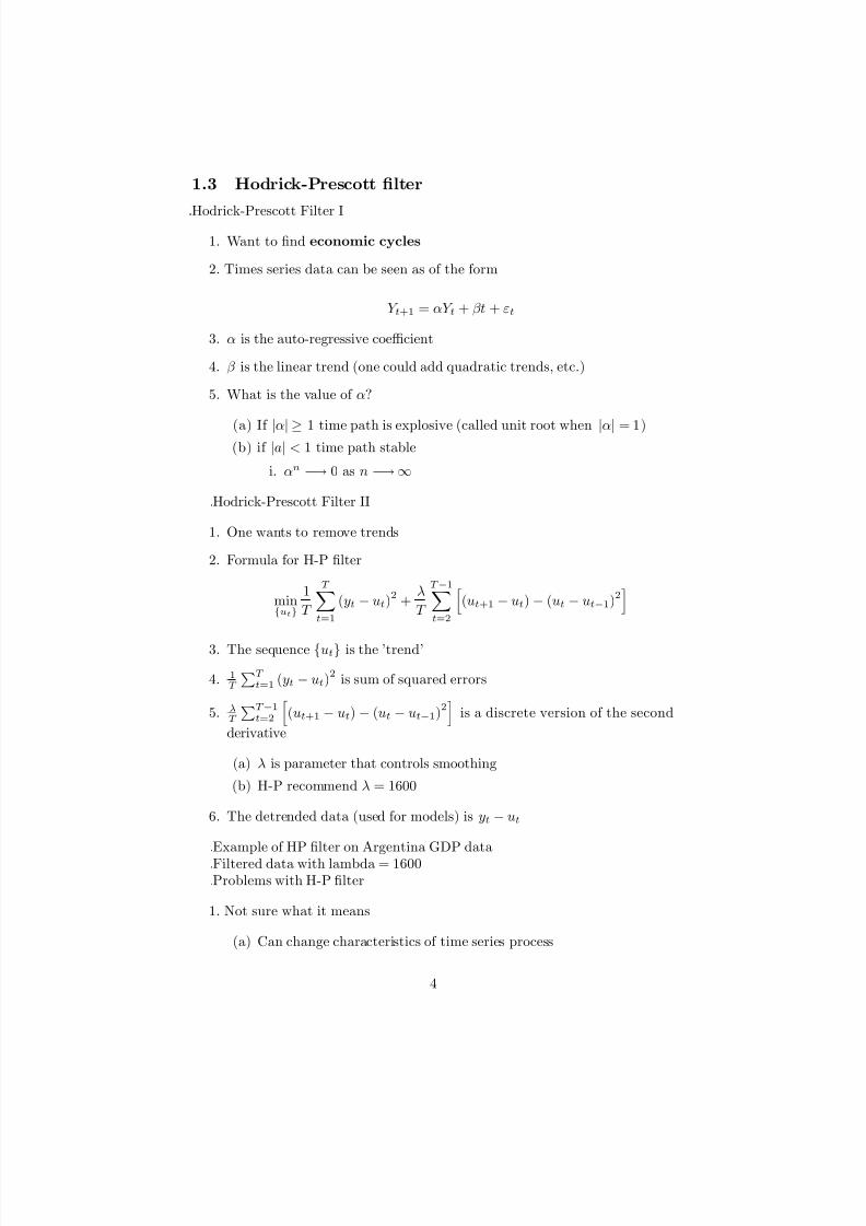
1.3 Hodrick-Prescott …lter

Hodrick-Prescott Filter I

1. Want to …nd economic cycles

2. Times series data can be seen as of the form

Y t+1 = Y t + t + "t

3. is the auto-regressive coe¢cient

4. is the linear trend (one could add quadratic trends, etc.)

5. What is the value of ?

(a) If jj 1 time path is explosive (called unit root when jj = 1)(b) if jaj < 1 time path stable

i. n ! 0 as n ! 1

Hodrick-Prescott Filter II

1. One wants to remove trends

2. Formula for H-P …lter

minfutg

1

T

T Xt=1

(yt ut)2 +

T

T 1Xt=2

h(ut+1 ut) (ut ut1)2

i

3. The sequence futg is the ’trend’

4. 1T

PT t=1 (yt ut)

2is sum of squared errors

5. T

PT 1t=2

h(ut+1 ut) (ut ut1)

2i

is a discrete version of the second

derivative

(a) is parameter that controls smoothing

(b) H-P recommend = 1600

6. The detrended data (used for models) is yt ut

Example of HP …lter on Argentina GDP data

Filtered data with lambda = 1600Problems with H-P …lter

1. Not sure what it means

(a) Can change characteristics of time series process

4



0 20 40 60 80 100 1201.8

2

2.2

2.4

2.6

2.8

3

3.2x 105

λ=10000

λ=200

λ=1600

Figure 1: Three Hodrick-Prescott …lters

0 20 40 60 80 100 120-0.5

0

0.5

1

1.5

2

2.5

3

3.5x 10

5

datafiltered data

cycles that remain (data thatwe use)

Figure 2: GDP data, HP trend, and detrended GDP data

5



(b) Removes certain (low) frequences from the process

(c) What does the data explain after the …ltering?2. Endpoint problems

(a) Because it is a weighed average of points

(b) At endpoints, only have one side of average

3. However, has become common practice to use H-P …lter

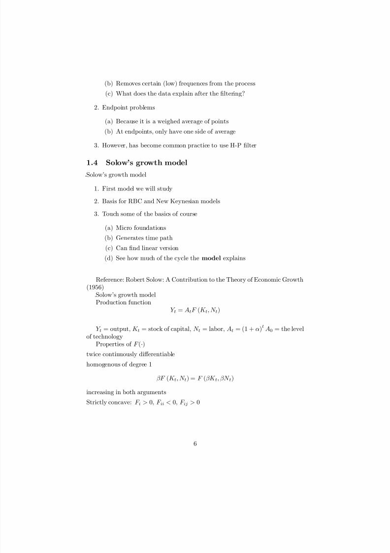
1.4 Solow’s growth model

Solow’s growth model

1. First model we will study

2. Basis for RBC and New Keynesian models

3. Touch some of the basics of course

(a) Micro foundations

(b) Generates time path

(c) Can …nd linear version

(d) See how much of the cycle the model explains

Reference: Robert Solow: A Contribution to the Theory of Economic Growth

(1956)Solow’s growth modelProduction function

Y t = AtF (K t;N t)

Y t = output, K t = stock of capital, N t = labor, At = (1 + )tA0 = the levelof technology

Properties of F ()

twice continuously di¤erentiable

homogenous of degree 1

F (K t; N t) = F (K t; N t)

increasing in both arguments

Strictly concave: F i > 0, F ii < 0, F ij > 0

6



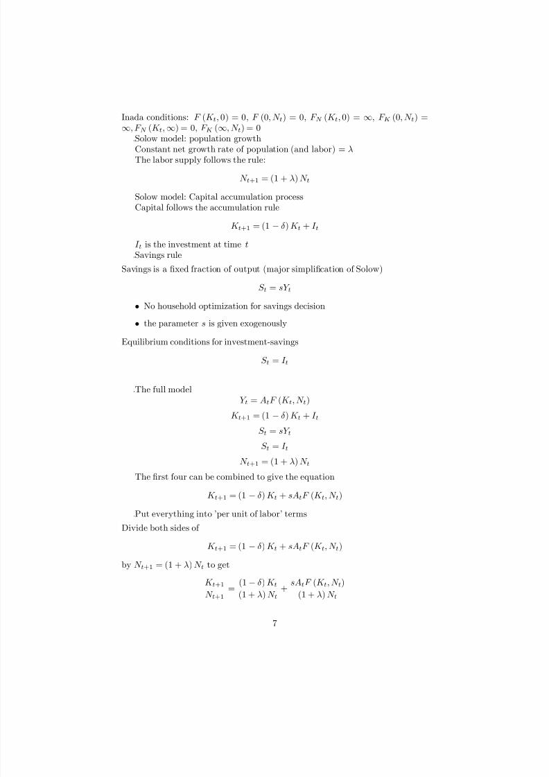
Inada conditions: F (K t; 0) = 0, F (0; N t) = 0, F N (K t; 0) = 1, F K (0; N t) =1; F N (K t;1) = 0, F K (1; N t) = 0

Solow model: population growthConstant net growth rate of population (and labor) = The labor supply follows the rule:

N t+1 = (1 + )N t

Solow model: Capital accumulation processCapital follows the accumulation rule

K t+1 = (1 )K t + I t

I t is the investment at time tSavings rule

Savings is a …xed fraction of output (major simpli…cation of Solow)

S t = sY t

No household optimization for savings decision

the parameter s is given exogenously

Equilibrium conditions for investment-savings

S t = I t

The full modelY t = AtF (K t;N t)

K t+1 = (1 )K t + I t

S t = sY t

S t = I t

N t+1 = (1 + )N t

The …rst four can be combined to give the equation

K t+1 = (1 )K t + sAtF (K t; N t)

Put everything into ’per unit of labor’ terms

Divide both sides of

K t+1 = (1 )K t + sAtF (K t; N t)

by N t+1 = (1 + )N t to get

K t+1N t+1

=(1 )K t(1 + )N t

+sAtF (K t; N t)

(1 + )N t

7



De…ning per-worker terms: kt = K t=N t, yt = Y t=N t, this can be written as

kt+1 = (1 )(1 + )

kt + sAt

(1 + )F (K t; N t)

N t

Because the production function is homogenous of degree 1,

F (K t;N t)

N t= F

K tN t

;N tN t

= F (kt; 1) f (kt) ;

The Solow di¤erence equation can be written as

kt+1 = G (kt) =(1 )

(1 + )kt +

sAt

(1 + )f (kt)

We will (in class) let At = A0, a constant technology

Model with constant technological growth

At = (1 + )tA0

where = 0

Using the Cobb-Douglas production function and zero technological growthf (kt) = A0k

t

The Solow …rst di¤erence equation is

kt+1 = bG (kt) =(1 )

(1 + )kt +

sA0

(1 + )kt

Given some initial k0, the time path for the economy can be found

Where the solution k to the equation

k = bG (k) =(1 )

(1 + )k +

sA0

(1 + )k

is a stationary state capital stock for the economy

1.5 Stability conditions for Solow ModelSolow Graph

[5cm]7cm5cm

Stability conditions for Solow model

8



0 1 2 3

0.0

0.5

1.0

1.5

2.0

2.5

kt

kt+1

Figure 3: Stability conditions

There are two stationary states

zero

at

k =

sA0

+

11

this last is an attractorA result of Solow ModelPoor countries (those with less capital) grow faster than richGross growth rate of capital can be written as

t =kt+1kt =

(1 )kt + sA0f (kt)

(1 + )kt :

And taking the derivative with respect to capital:

d tdkt

=sA0

(1 + )k2t[f 0(kt)kt f (kt)] < 0

when kt > 0.

Countries with higher kt have smaller growth rates of capitalStochastic variables

A probability space: (;F ;P )

– is a set that contains all possible states of nature that might occur

What is a state of nature

– F is a collection of subsets of

Why do we need this?

– P is a probability measure over F

Some draw from is observed each period

9



2 A stochastic Solow Model

A stochastic Solow ModelSuppose that technology is stochastic,

At = Ae"t

A is positive

random term "t has a normal distribution with mean zero

So in stationary state (with "t = 0), e"t = 1

e"t is never negative

The stochastic version of the Solow …rst order di¤erence equation is

kt+1 =

(1 )kt + sAe"tf (kt)

(1 + ):

Version in Logs (model is simpler this way)

1. Divide both sides by kt

2. replace kt+1=kt by growth rate t

3. There is a problem with ln

(1 )kt + sAe"tf (kt)

4. Take logs of both sides

ln

t

1

1 +

= ln

sA

(1 + n)+ ln

f (kt)

kt+ "t:

5. Use Cobb-Douglas production function, f (kt) = kt , to get

ln

t

1

1 +

= ' (1 ) ln kt + "t;

where ' lnsA=(1 + )

Simulation of stochastic Solow model[5cm]8cm

5cmParameters usedA = 1

s = :2 = :02 = :1 = :362" =:2Log-linear version of (no growth trend) Solow model

10



Figure 4: Three simulations of the exact Solow model

1. We have a second way to handle dynamics

2. Make an (log) linear approximation of the model

3. Study the dynamics of this linear model

4. Exists technology for solving dynamic linear models

Log-linear version of (no growth trend) Solow model

1. Begin with the Solow di¤erence equation

(1 + )kt+1 = (1 )kt + sAe"tkt ;

2. De…ne ekt = ln(kt k), where k is the stationary state value of capital

3. Then kt = keekt

4. The Solow di¤erence equation is now

(1 + ) keekt+1 = (1 )ke

ekt + sAe"tkeekt ;

5. Use the approximation that for small

ekt,

eaekt = 1 + aekt6. This approximation comes from a …rst order Taylor expansion of ea

ekt

Log-linear Solow model

11



1. The approximation of

(1 + ) keekt+1 = (1 )keekt + sAkeekt+e"

t ;

(note that e"teekt = e

ekt+e"t

) is

(1 + ) k

1 + ekt+1 = (1 )k

1 + ekt + sAk

1 + ekt + e"t:

2. The 1’s in parenthisis drop out because

(1 + ) k = (1 )k + sAk:

3. The log-linear version of the model is

(1 + )kekt+1 = h(1 )k + sAk

i ekt + sAk

e"t :

Log-linear Solow model (continued)

1. This further simpli…es (since + = sAk1

) to

ekt+1 =1 + ( + )

1 + ekt +

+

1 + e"t :

2. Notice that

(1 ) + ( + )

1 + =

1 + (1 )

1 + < 1

3. Let B = 1+(1)1+ and C = +

1+ < 1 and time t + 1 capital is equal to

ekt+1 = C 1Xi=0

Bi"ti

This is a convergent sequence

Variance of capital

The variance of time t + 1 capital is equal to

var ekt+1 = E ekt+12 = E C 1

Xi=0Bi

"ti!C 1

Xi=0Bi

"ti!= C 2E

1Xi=0

Bi"ti

!1Xi=0

Bi"ti

!

12



Figure 5: Simulations of the exact and log-linear Solow model

Since the shocks are independent, E ("i"j) = 0 if i 6= j, and = 2 if i = j. Allcross terms drop out and the sums become

varekt+1 = C 22E

1Xi=0

B2i =C 2

1 B22

Using the parameters given before, B = 0:971 76 and C = :04411 8 so that

varekt+1 =

(:04411 8)2

1 (0:97176)22 = :0249552

The variance of capital is very small compared to the technology shock varianceTime path of capital (comparing approximate to exact models)Variance of output

1. Output comes from the equation

yt = Atkt = Ae"tkt

2. A log-linear approximation of this is

y (1 + eyt) yeeyt = Akeekt+"t Ak

1 + ekt + "t

which simpli…es to eyt ekt + "t

13



The variance of output is almost entirely made up of variance in technology.The e¤ect of changes in the capital stock are very small

Solow model does not explain the persistence of shocks (cycles) in an economyHomework1. 1. Usando un modelo de Solow con crecimiento en tecnologia de

At = (1 + )tA0

con A0 = 5 y = :01, encuentre los caminos de capital y de producto per capitapor 25 periodo cuando k(0) = :1 y cuando k(0) = 40. Gra…ce los.caminos decapital Usa s = :15, = :57, y = :018. (Nota: debe usar Matlab para estaproblema).

2. Muestre los gra…cos de los las tasas de crecimiento de capitalen problema1.

3. Describe the time path for a Solow model where there is an externalityfor each …rm and each …rm has the production function

yjt = Atkth

1t K 1t :

Lower case letters are for the …rm and upper case letters are for the economy asa whole. The total capital in the economy functions as an externality for each…rm.

14

1 solow model

Documents