progress in nonlinear differential...

Progress in Nonlinear Differential Equationsand Their ApplicationsVolume 75

Editor

Haim BrezisUniversité Pierre et Marie CurieParisandRutgers UniversityNew Brunswick, N.J.

Editorial Board

Antonio Ambrosetti, Scuola Internazionale Superiore di Studi Avanzati, TriesteA. Bahri, Rutgers University, New BrunswickFelix Browder, Rutgers University, New BrunswickLuis Cafarelli, Institute for Advanced Study, PrincetonLawrence C. Evans, University of California, BerkeleyMariano Giaquinta, University of PisaDavid Kinderlehrer, Carnegie-Mellon University, PittsburghSergiu Klainerman, Princeton UniversityRobert Kohn, New York UniversityP.L. Lions, University of Paris IXJean Mahwin, Université Catholique de LouvainLouis Nirenberg, New York UniversityLambertus Peletier, University of LeidenPaul Rabinowitz, University of Wisconsin, MadisonJohn Toland, University of Bath

Differential Equations, Chaos and Variational Problems

Vasile StaicuEditor

BirkhäuserBasel · Boston · Berlin

2000 Mathematics Subject Classification: 34, 35, 37, 39, 45, 49, 58, 70, 76, 80, 91, 93

Library of Congress Control Number: 2007935492

Bibliographic information published by Die Deutsche BibliothekDie Deutsche Bibliothek lists this publication in the Deutsche Nationalbibliografie; detailed bibliographic data is available in the Internet at <http://dnb.ddb.de>.

ISBN 978-3-7643-8481-4 Birkhäuser Verlag AG, Basel · Boston · Berlin

This work is subject to copyright. All rights are reserved, whether the whole or part of the material is concerned, specifically the rights of translation, reprinting, re-use of illustrations, broadcasting, reproduction on microfilms or in other ways, and storage in data banks. For any kind of use whatsoever, permission from the copyright owner must be obtained.

© 2008 Birkhäuser Verlag AG Basel · Boston · Berlin P.O. Box 133, CH-4010 Basel, SwitzerlandPart of Springer Science+Business MediaPrinted on acid-free paper produced from chlorine-free pulp. TCF ∞Printed in Germany

ISBN 978-3-7643-8481-4 e-ISBN 978-3-7643-8482-1

9 8 7 6 5 4 3 2 1 www.birkhauser.ch

Editor:Vasile StaicuDepartment of Mathematics University of Aveiro3810-193 AveiroPortugal

e-mail: [email protected]

Contents

Editorial Introduction . . . . . . . . . . . . . . . . . . . . . . . . . . . . . . . . . . . . . . . . . . . . . . . . . . . . . . ix

R.P. Agarwal, M.E. Filippakis, D. O’Regan and N. S. PapageorgiouNodal and Multiple Constant Sign Solution for Equations with thep-Laplacian . . . . . . . . . . . . . . . . . . . . . . . . . . . . . . . . . . . . . . . . . . . . . . . . . . . . . . . 1

Z. ArtsteinA Young Measures Approach to Averaging . . . . . . . . . . . . . . . . . . . . . . . . 15

J.-P. Aubin and P. Saint-PierreViability Kernels and Capture Basins for Analyzing the DynamicBehavior: Lorenz Attractors, Julia Sets, and Hutchinson’s Maps . . . 29

R. BaierGeneralized Steiner Selections Applied to Standard Problems ofSet-Valued Numerical Analysis . . . . . . . . . . . . . . . . . . . . . . . . . . . . . . . . . . . . 49

S. BianchiniOn the Euler-Lagrange Equation for a Variational Problem . . . . . . . . 61

A. BressanSingular Limits for Impulsive Lagrangian Systems with DissipativeSources . . . . . . . . . . . . . . . . . . . . . . . . . . . . . . . . . . . . . . . . . . . . . . . . . . . . . . . . . . . 79

P. Cannarsa, H. Frankowska and E.M. MarchiniLipschitz Continuity of Optimal Trajectories in DeterministicOptimal Control . . . . . . . . . . . . . . . . . . . . . . . . . . . . . . . . . . . . . . . . . . . . . . . . . . 105

C. Carlota and A.OrnelasAn Overview on Existence of Vector Minimizers for Almost Convex1−dim Integrals . . . . . . . . . . . . . . . . . . . . . . . . . . . . . . . . . . . . . . . . . . . . . . . . . . . 117

A. CellinaStrict Convexity, Comparison Results and Existence of Solutions toVariational Problems . . . . . . . . . . . . . . . . . . . . . . . . . . . . . . . . . . . . . . . . . . . . . . 123

vi Contents

A. CerneaNecessary Optimality Conditions for Discrete Delay Inclusions . . . . 135

F. ClarkeNecessary Conditions in Optimal Control and in the Calculus ofVariations . . . . . . . . . . . . . . . . . . . . . . . . . . . . . . . . . . . . . . . . . . . . . . . . . . . . . . . . . 143

C. CorduneanuAlmost Periodicity in Functional Equations . . . . . . . . . . . . . . . . . . . . . . . 157

A. Dawidowicz and A. PoskrobkoAge-dependent Population Dynamics with the Delayed Argument . 165

R. Dilao and R. Alves-PiresChaos in the Stormer Problem . . . . . . . . . . . . . . . . . . . . . . . . . . . . . . . . . . . . 175

F. Ferreira, A.A. Pinto, and D.A. RandHausdorff Dimension versus Smoothness . . . . . . . . . . . . . . . . . . . . . . . . . . 195

A. Gavioli and L. SanchezOn Bounded Trajectories for Some Non-Autonomous Systems . . . . . 211

E. Girejko and Z. BartosiewiczOn Generalized Differential Quotients and Viability . . . . . . . . . . . . . . . 223

R. Goncalves, A.A. Pinto, and F. CalheirosNonlinear Prediction in Riverflow – the Paiva River Case . . . . . . . . . . 231

J. Kennedy and J.A. YorkeShadowing in Higher Dimensions . . . . . . . . . . . . . . . . . . . . . . . . . . . . . . . . . . 241

J. MawhinBoundary Value Problems for Nonlinear Perturbations of Singularφ-Laplacians . . . . . . . . . . . . . . . . . . . . . . . . . . . . . . . . . . . . . . . . . . . . . . . . . . . . . . 247

F.M. MinhosExistence, Nonexistence and Multiplicity Results for Some BeamEquations . . . . . . . . . . . . . . . . . . . . . . . . . . . . . . . . . . . . . . . . . . . . . . . . . . . . . . . . . 257

St. MiricaReducing a Differential Game to a Pair of Optimal ControlProblems . . . . . . . . . . . . . . . . . . . . . . . . . . . . . . . . . . . . . . . . . . . . . . . . . . . . . . . . . 269

B. S. MordukhovichOptimal Control of Nonconvex Differential Inclusions . . . . . . . . . . . . . . 285

Contents vii

F. Mukhamedov and J. F. F. MendesOn Chaos of a Cubic p-adic Dynamical System . . . . . . . . . . . . . . . . . . . . 305

J. MyjakSome New Concepts of Dimension . . . . . . . . . . . . . . . . . . . . . . . . . . . . . . . . . 317

R. OrtegaDegree and Almost Periodicity . . . . . . . . . . . . . . . . . . . . . . . . . . . . . . . . . . . . 345

M. OtaniL∞-Energy Method, Basic Tools and Usage . . . . . . . . . . . . . . . . . . . . . . . 357

B. RicceriSingular Set of Certain Potential Operators in Hilbert Spaces . . . . . 377

J.M.R. SanjurjoShape and Conley Index of Attractors and Isolated Invariant Sets . 393

M.R. Sidi Ammi and D. F.M. TorresRegularity of Solutions for the Autonomous Integrals of theCalculus of Variations . . . . . . . . . . . . . . . . . . . . . . . . . . . . . . . . . . . . . . . . . . . . . 407

S. TerraciniMulti-modal Periodic Trajectories in Fermi–Pasta–Ulam Chains . . . 415

S. Zambrano and M. A. F. SanjuanControl of Transient Chaos Using Safe Sets in Simple DynamicalSystems . . . . . . . . . . . . . . . . . . . . . . . . . . . . . . . . . . . . . . . . . . . . . . . . . . . . . . . . . . . 425

Editorial Introduction

This book is a collection of original papers and state-of-the-art contributions writ-ten by leading experts in the areas of differential equations, chaos and variationalproblems in honour of Arrigo Cellina and James A. Yorke, whose remarkable sci-entific carrier was a source of inspiration to many mathematicians, on the occasionof their 65th birthday.

Arrigo Cellina and James A. Yorke were born on the same day: August 3,1941. Both received their Ph.D. degrees from the University of Maryland, wherethey met first in the late 1960s, at the Institute for Fluid Dynamics and AppliedMathematics. They had offices next to each other and though they were of thesame age, Yorke was already Assistant Professor, while Cellina was a GraduateStudent. Each one of them had a small daughter, and this contributed to theirfriendship.

Arrigo Cellina James A. YorkeYorke arrived at the office every day with a provision of cans of Coca Cola,

his daily ration, that he put in the air conditioning fan, to keep cool. Cellina saysthat he was very impressed by Yorke’s way of doing mathematics; Yorke couldprove very interesting new results using almost elementary mathematical tools,little more than second year Calculus.

From those years, he remembers for example the article Noncontinuable so-lutions of differential-delay equations where Yorke shows, in an elementary waybut with a clever use of the extension theorem, that the basic theorem of continu-ation of solutions to ordinary differential equations cannot be valid for functional

x Editorial Introduction

equations (at that time very fashionable). In the article A continuous differen-tial equation in Hilbert space without existence, Yorke gave the first example ofthe nonexistence of solutions to Cauchy problems for an ordinary differential in aHilbert space. Furthermore, in a joint paper with one of his students, Saperstone,he proved a controllability theorem without using the hypothesis that the originbelongs to the interior of the set of controls. This is just a sample of importantproblems to which Yorke made nontrivial contributions.

Yorke went around always carrying in his pocket a notebook where he anno-tated the mathematical problems that seemed important for future investigation.In those years Yorke’s collaboration with Andrezj Lasota began, which producedoutstanding results in the theory of “chaos”. Yorke became famous even in non-mathematical circles for his mathematical model for the spread of gonorrhoea.While traditional models were not in accord with experimental data, he proposeda simple model based on the existence of two groups of people and proved that thismodel fits well the experimental data. Later, in a 1975 paper entitled Period threeimplies chaos with T.Y. Lee, Yorke introduced a rigorous mathematical definitionof the term “chaos” for the study of dynamical systems. From then on, he played aleading role in the further research on chaos, including its control and applications.

Yorke’s goals to explore interdisciplinary mathematics were fully realized af-ter he earned his Ph.D. and joined the faculty of the Institute for Physical Scienceand Technology (IPST), an institute established in 1950 to foster excellence ininterdisciplinary research and education at the University of Maryland. He said:All along the goal of myself and my fellow researchers here at Maryland has beento find the concepts that the applied scientist needs. His chaos research group in-troduced many basic concepts with exotic names like crises, the control of chaos,fractal basin boundary, strange non-chaotic attractors, and the Kaplan–Yorke di-mension. One remarkable application of Yorke’s theory of chaos has been theweather prediction.

In 2003 Yorke shared with Benoit Mandelbrot of Yale University the prize forScience and Technology of Complexity of the Science and Technology Foundationof Japan for the Creation of Universal Concepts in Complex Systems-Chaos andFractals. With this prize, Jim Yorke was recognized for his outstanding achieve-ments in nonlinear dynamics that have greatly advanced the frontiers of scienceand technology.

Yorke’s research has been highly influential, with some of his papers receivinghundreds of citations. He is the author of three books on chaos, of a monographon gonorrhoea epidemiology, and of more than 300 papers in the areas of ordinarydifferential equations, dynamical systems, delay differential equations, applied andrandom dynamical systems.

He believes that a Ph.D. in mathematics is a licence to investigate the uni-verse, and he has supervised over 40 Ph.D. dissertations in the departments ofmathematics, physics and computer science.

Editorial Introduction xi

Currently, Jim Yorke is a Distinguished University Professor of Mathemat-ics and Physics, and Chair of the Mathematics Department of the University ofMaryland.

Arrigo Cellina received a Ph.D. degree in mathematics in 1968 and went backto Italy, where he was Assistant Professor and then Full Professor at the Univer-sities of Perugia, Florence, and Padua, at the International School for AdvancedStudies (SISSA) in Trieste, and at the University of Milan. He was a member ofthe scientific committee and then Director (1999–2001) of the International Math-ematical Summer Centre (CIME) in Florence, Italy, and also a member of thescientific council of CIM (International Centre for Mathematics) seated in Coim-bra, Portugal. Presently he is Professor at the University of Milan “Bicocca” andcoordinator of the Doctoral Program of this university.

In Italy, the International School for Advanced Studies (SISSA) was estab-lished in 1978, in Trieste, as a dedicated and autonomous scientific institute todevelop top-level research in mathematics, physics, astrophysics, biology and neu-roscience, and to provide qualified graduate training to Italian and foreign laure-ates, to train them for research and academic teaching.

SISSA was the first Italian school to set up post-laurea courses aimed at aPh. D. degree (Doctor Philosophiae). Cellina was one of the professors, foundersand, for several years, the Coordinator of the Sector of Functional Analysis andApplications at SISSA, from 1978 until 1996.

I was lucky to have been initiated to mathematical research on Aubin–Cellina’s book Differential inclusions in a research seminar at the University ofBucharest. Three years later I began my Ph.D. studies on differential inclusions atSISSA, under the supervision of Arrigo Cellina. I arrived at SISSA coming fromFlorence where I spent a very rewarding and training period of one year as a Re-search Fellow of GNAFA under the supervision of Roberto Conti, and I rememberthat Arrigo welcomed me with a kindness equal to his erudition.

Always available to discuss and to help his students to overcome difficulties,not only of mathematical orders, Arrigo taught me a lot more than differentialinclusions. I remember with great pleasure his beautiful lessons, the long hours ofreflection in front of the blackboard in his office, as well as the walks along the seaor in the park of Miramare.

I remember SISSA of those days as a very exciting environment. A communityof researchers worked there, while several others were visiting SISSA and gaveshort courses or seminars concerning their new results. The Sector of FunctionalAnalysis and Applications was located in a beautiful place, close to the Castle ofMiramare, and near the International Centre for Theoretical Physics (ICTP), withan excellent library where we could spend much of our time. Without a doubt,this has been a very fruitful and rewarding period of my life, both as a scientificand as a life experience. Cellina’s contribution has been significant.

Cellina’s scientific work has always been highly original, introducing entirelynew techniques to attack the difficult problems he considered. He introduced thenotion of graph approximate selection for upper semicontinuous multifunctions,

xii Editorial Introduction

thus establishing a basic connection between ordinary differential inclusions anddifferential inclusions. He also introduced the fixed-point approach to prove the ex-istence of differential inclusions based on continuous selections from multifunctionswith decomposable values.

The Baire category method, for the analysis of differential inclusions withoutconvexity assumptions, has been developed starting from Cellina’s seminal paperOn the differential inclusion x′ ∈ [−1, 1], published in 1980 by the Rendicontidell’Academia dei Lincei. Eventually this method recently found applications toproblems of the Calculus of Variations, without convexity or quasi-convexity as-sumptions, as well as to implicit differential equations. This year, it found evenmore striking new applications to the construction of deep counterexamples in thetheory of multidimensional fluid flow.

More recently, Cellina’s research activity was devoted to the area of the Cal-culus of Variations, where he obtained important results on the validity of theEuler-Lagrange equation, on the regularity of minimizers, on necessary and suffi-cient conditions for the existence of minima, and on uniqueness and comparisonof minima without strict convexity.

The book Differential Inclusions, co-authored by Cellina with J. P. Aubin andpublished by Springer, as well as several of his eighty papers published in first-class journals, are now classic references to their subject. Cellina also edited severalvolumes with lectures and seminars of CIME sessions, published by Springer inthe subseries Fondazione C.I.M.E. of the Lecture Notes in Mathematics series.

Cellina mentored ten Ph.D. students: seven of them while at SISSA andthree others at the university of Milan. Among his former students, many are nowProfessors in prestigious universities in Italy, Portugal, Chile or other countries.Several more mathematicians continue to be inspired by his ground-breaking ideas.

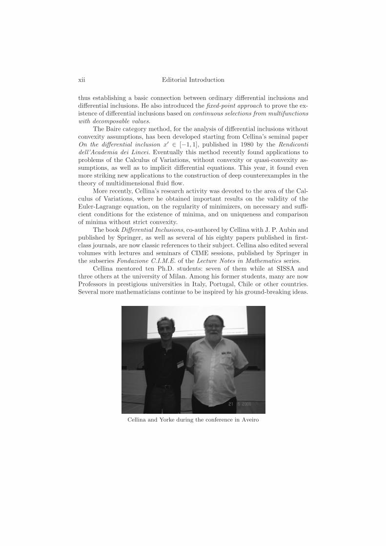
Cellina and Yorke during the conference in Aveiro

Editorial Introduction xiii

In June 2006, I had the privilege to organize in Aveiro (Portugal) with mycolleagues from the Functional Analysis and Applications research group, the con-ference Views on ODEs, in celebration of the 65th birthday of Arrigo Cellina andJames A. Yorke. Several friends, former students and collaborators, presently lead-ing experts in differential equations, chaos and variational problems, gathered inAveiro on this occasion to discuss their new results. The present volume collectsthirty-two original papers and state-of-the-art contributions of participants to thisconference and brings the reader to the frontier of research in these modern fieldsof research.

I wish to thank Professor Haim Brezis for accepting to publish this bookas a volume of the series Progress in Nonlinear Differential Equations and TheirApplications. I also thank Thomas Hempfling for the professional and pleasant col-laboration during the preparation of this volume. Finally, I gratefully acknowledgepartial financial support from the Portuguese Foundation for Science and Technol-ogy (FCT) under the Project POCI/MAT/55524/2004 and from the Mathematicsand Applications research unit of the University of Aveiro.

Aveiro, October 2007 Vasile Staicu

Progress in Nonlinear Differential Equationsand Their Applications, Vol. 75, 1–14c© 2007 Birkhauser Verlag Basel/Switzerland

Nodal and Multiple Constant Sign Solution forEquations with the p-Laplacian

Ravi P. Agarwal, Michael E. Filippakis,Donal O’Regan, and Nikolaos S. Papageorgiou

Dedicated to Arrigo Cellina and James Yorke

Abstract. We consider nonlinear elliptic equations driven by the p-Laplacianwith a nonsmooth potential (hemivariational inequalities). We obtain the ex-istence of multiple nontrivial solutions and we determine their sign (one posi-tive, one negative and the third nodal). Our approach uses nonsmooth criticalpoint theory coupled with the method of upper-lower solutions.

Mathematics Subject Classification (2000). 35J60, 35J70.

Keywords. Scalar p-Laplacian, eigenvalues, (S)+-operator, local minimizer,positive solution, nodal solution.

1. Introduction

Let Z ⊆ RN be a bounded domain with a C2-boundary ∂Z. We consider thefollowing nonlinear elliptic problem with nonsmooth potential (hemivariationalinequality): {

−div(‖Dx(z)‖p−2Dx(z)

)∈ ∂j

(z, x(z)

)a.e. on Z ,

x|∂Z = 0, 1 < p < ∞ .

}(1.1)

Here j(z, x) is a measurable function on Z×R and x → j(z, x) is locally Lip-schitz and in general nonsmooth. By ∂j(z, ·) we denote the generalized subdifferen-tial of j(z, ·) in the sense of Clarke [3]. The aim of this lecture is to produce multiplenontrivial solutions for problem (1.1) and also determine their sign (positive, neg-ative or nodal (sign-changing) solutions). Recently this problem was studied forequations driven by the p-Laplacian with a C1-potential function (single-valued

Researcher M. E. Filippakis supported by a grant of the National Scholarship Foundation ofGreece (I.K.Y.).

2 R.P. Agarwal, M. E. Filippakis, D. O’Regan, and N. S. Papageorgiou

right hand side), by Ambrosetti-Garcia Azorero-Peral Alonso [1], Carl-Perera [2],Garcia Azorero-Peral Alonso [7], Garcia Azorero-Manfredi-Peral Alonso [8], Zhang-Chen-Li [15] and Zhang-Li [16]. In [1], [7], [8], the authors consider certain nonlin-ear eigenvalue problems and obtain the existence of two strictly positive solutionsfor all small values of the parameter λ ∈ R (i.e., for all λ ∈ (0, λ∗)). In [2], [15], [16]the emphasis is on the existence of nodal (sign changing) solutions. Carl-Perera [2]extend to the p-Laplacian the method of Dancer-Du [6], by assuming the existenceof an ordered pair of upper-lower solutions. In contrast, Zhang-Chen-Li [15] andZhang-Li [16], base their approach on the invariance properties of certain carefullyconstructed pseudogradient flow. Our approach here is closer to that of Dancer-Du [6] and Carl-Perera [2], but in contrast to them, we do not assume the existenceof upper-lower solutions, but instead we construct them and we use a recent alter-native variational characterization of the second eigenvalue λ2 of (−�p,W

1,p0 (Z))

due to Cuesta-de Figueiredo-Gossez [5], together with a nonsmooth version of thesecond deformation theorem due to Corvellec [4].

2. Mathematical background

Let X be a Banach space and X∗ its topological dual. By 〈, ·, ·〉 we denote theduality brackets for the pair (X,X∗). Let ϕ : X → R be a locally Lipschitz. Thegeneralized directional derivative ϕ0(x;h) of ϕ at x ∈ X in the direction h ∈ X, isgiven by

ϕ0(x;h) = lim supx′ → xλ ↓ 0

ϕ(x′ + λh)− ϕ(x′)λ

.

The function h → ϕ0(x;h) is sublinear continuous and so it is the supportfunction of a nonempty, convex and w∗-compact set ∂ϕ(x) ⊆ X∗ defined by

∂ϕ(x) ={x∗ ∈ X∗ : 〈x∗, h〉 ≤ ϕ0(x;h) for all h ∈ X

}.

The multifunction x → ∂ϕ(x) is known as the generalized subdifferentialor subdifferential in the sense of Clarke. If ϕ is continuous convex, then ∂ϕ(x)coincides with the subdifferential in the sense of convex analysis. If ϕ ∈ C1(X),then ∂ϕ(x) = {ϕ′(x)}. We say that x ∈ X is a critical point of ϕ, if 0 ∈ ∂ϕ(x).The main reference for this subdifferential, is the book of Clarke [3].

Given a locally Lipschitz function ϕ : X → R, we say that ϕ satisfies thenonsmooth Palais-Smale condition at level c ∈ R (the nonsmooth PSc-conditionfor short), if every sequence {xn}n≥1 ⊆ X such that ϕ(xn) → c and m(xn) =inf{‖x‖ : x∗ ∈ ∂ϕ(xn)} → 0 as n →∞, has a strongly convergent subsequence. Ifthis is true at every level c ∈ R, then we say that ϕ satisfies the PS-condition.

Definition 2.1. Let Y be a Hausdorff topological space and E0, E,D nonempty,closed subsets of Y with E0 ⊆ E. We say that {E0, E} is linking with D in Y , ifthe following hold:(a) E0 ∩D = ∅;

Nodal solutions 3

(b) for any γ ∈ C(E, Y ) such that γ|E0 = id|E0 , we have γ(E) ∩D = ∅.Using this geometric notion, we can have the following minimax characteri-

zation of critical values for nonsmooth, locally Lipschitz functions (see Gasinski-Papageorgiou [9], p.139).

Theorem 2.2. If X is a Banach space, E0, E,D are nonempty, closed subsets ofX, {E0, E} are linking with D in X, ϕ : X → R is locally Lipschitz, sup

E0

< infD

ϕ,

Γ = {γ ∈ C(E,X) : γ|E0 = id|E0}, c = infγ∈Γ

supv∈E

ϕ(γ(v)) and ϕ satisfies the

nonsmooth PSc-condition, then c ≥ infD

ϕ and c is a critical value of ϕ.

Remark 2.3. By appropriate choices of the linking sets {E0, E,D}, from The-orem 2.2, we obtain nonsmooth versions of the mountain pass theorem, saddlepoint theorem, and generalized mountain pass theorem. For details, see Gasinksi-Papageorgiou [9].

Given a locally Lipschitz function ϕ : X → R, we set

ϕ·c ={x ∈ X : ϕ(x) < c

}(the strict sublevel set of ϕ at c ∈ R)

and Kc ={x ∈ X : 0 ∈ ∂ϕ(x), ϕ(x) = c

}(the critical points of ϕ at the level c).

The next theorem is a nonsmooth version, of the so-called “second deforma-tion theorem” (see Gasinski-Papageorgiou [10], p.628) and it is due to Corvellec [4].

Theorem 2.4. If X is a Banach space, ϕ : X → R is locally Lipschitz, it satisfiesthe nonsmooth PS-condition, a ∈ R, b ∈ R ∪ {+∞}, ϕ has no critical pointsin ϕ−1(a, b) and Ka is discrete nonempty and contains only local minimizers of ϕ,

then there exists a deformation h : [0, 1]× ϕ·b → ϕ·b such that(a) h(t, ·)|Ka

= Id|Kafor all t ∈ [0, 1];

(b) h(t, ϕ·b) ⊆ ϕ·a ∪Ka;(c) ϕ(h(t, x)) ≤ ϕ(x) for all (t, x) ∈ [0, 1]× ϕ·b.

Remark 2.5. In particular then ϕ·b ∪Ka is a weak deformation retract of ϕ·b.

Let us mention a few basic things about the spectrum of (−�p,W1,p0 (Z)),

which we will need in the sequel. So let m ∈ L∞(Z)+, m = 0 and consider thefollowing weighted eigenvalue problem:{

−div(‖Dx(z)‖p−2Dx(z)

)= λm(z)|x(z)|p−2x(z) a.e. on Z ,

x|∂Z = 0, 1 < p < ∞ .

}(2.1)

Problem (2.1) has at least eigenvalue λ1(m) > 0, which is simple, isolated andadmits the following variational characterization in terms of the Rayleigh quotient:

λ1(m) = min

[‖Dx‖p

p∫Z

m|x|pdz: x ∈ W 1,p

0 (Z) , x = 0

](2.2)

The minimum is attained on the corresponding one dimensional eigen-space E(λ1). By u1 we denote the normalized eigenfunction, i.e.,

∫Z

m|u1|pdz = 1


(if m ≡ 1, then ‖u1‖p = 1). We have E(λ1) = Ru1 and u1 ∈ C10 (Z) (nonlinear

regularity theory, see Lieberman [13] and Gasinski-Papageorgiou [10], p.738). Weset

C+ ={x ∈ C1

0 (Z) : x(z) ≥ 0 for all z ∈ Z}

and intC+ ={

x ∈ C+ : x(z) > 0 for all z ∈ Z and∂x

∂n(z) < 0 for all z ∈ ∂Z

}.

The nonlinear strong maximum principle of Vazquez [14], implies that u1 ∈intC+.

Since λ1(m) is isolated, we can define the second eigenvalue of (−�p,W 1,p

0 (Z),m) by

λ∗2(m) = inf

[λ : λ is an eigenvalue of (2.1), λ = λ1(m)

]> λ1(m) .

Also by virtue of the Liusternik-Schnirelmann theory, we can find an increas-ing sequence of eigenvalues {λk(m)}k≥1 such that λk(m) → ∞. These are theso-called LS-eigenvalues. We have

λ2

∗(m) = λ2(m) ,

i.e., the second eigenvalue and the second LS-eigenvalue coincide. The eigen-values λ1(m) and λ2(m) exhibit the following monotonicity properties with respectto the weight function m ∈ L∞(Z)+ :

– If m1(z) ≤ m2(z) a.e. on Z, and m1 = m2, then λ1(m2) < λ1(m1) (see (2.2)).– If m1(z) < m2(z) a.e. on Z, then λ2(m2) < λ2(m1).

If m ≡ 1, then we write λ1(1) = λ1 and λ2(1) = λ2. Recently Cuesta-deFigueiredo-Gossez [5], produced the following alternative variational characteriza-tion of λ2 :

λ2 = infγ0∈Γ0

supx∈γ0([−1,1])‖Dx‖pp (2.3)

with Γ0 = {γ0 ∈ C([−1, 1], S) : γ0(−1) = −u1, γ0(1) = u1}, S = W 1,p0 (Z) ∩

∂BLp(Z)1 and ∂B

Lp(Z)1 = {x ∈ Lp(Z) : ‖x‖p = 1}.

Finally we recall the notions of upper and lower solution for problem (1.1).Definition 2.6.

(a) A function x ∈ W 1,p(Z) is an upper solution of (1.1), if x|∂Z ≥ 0 and∫Z

‖Dx‖p−2(Dx,Dv)RNdz ≥∫

Z

uvdz

for all v ∈ W 1,p0 (Z), v ≥ 0 and all u ∈ Lη(Z), u(t) ∈ ∂j(t, x(z)) a.e. on Z

for some 1 < η < p∗.(b) A function x ∈ W 1,p(Z) is a lower solution of (1.1), if x|∂Z ≤ 0 and∫

Z

‖Dx‖p−2(Dx,Dv)RNdz ≤∫

Z

uvdz

Nodal solutions 5

for all v ∈ W 1,p0 (Z), v ≥ 0 and all u ∈ Lη(Z), u(z) ∈ ∂j(z, x(z)) a.e. on Z

for some 1 < η < p∗.

3. Multiple constant sign solutions

In this section, we produce multiple solutions of constant sign. Our approach isbased on variational techniques, coupled with the method of upper lower solutions.We need the following hypotheses on the nonsmooth potential j(z, x).

H(j)1: j : Z ×R → R is a function such that j(t, 0) = 0 and ∂j(z, 0) = {0} a.e. onZ, and

(i) for all x ∈ R, z → j(z, x) is measurable;(ii) for almost all z ∈ Z, x → j(z, x) is locally Lipschitz;(iii) for a.a. z ∈ Z, all x ∈ R and all u ∈ ∂j(z, x), we have

|u| ≤ a(z) + c|x|p−1 with a ∈ L∞(Z)+, c > 0 ;

(iv) there exists θ ∈ L∞(Z)+, θ(z) ≤ λ1 a.e. on Z, θ = λ1 such that

lim sup|x|→∞

u

|x|p−2x≤ θ(z)

uniformly for a.a. z ∈ Z and all u ∈ ∂j(z, x) ;(v) there exists η, η ∈ L∞(Z)+ , λ1 ≤ η(z) ≤ η(z) a.e. on Z, λ1 = η such

that

η(z) ≤ lim infx→0

u

|x|p−2x≤ lim sup

x→0

u

|x|p−2x≤ η(z)

uniformly for a.a. z ∈ Z and all u ∈ ∂j(z, x);(vi) for a.a. z ∈ Z, all x ∈ R and all u ∈ ∂j(z, x), we have ux ≥ 0 (sign

condition).Let ε > 0 and γε ∈ L∞(Z)+, γε = 0 and consider the following auxiliary

problem:{−div

(‖Dx(z)‖p−2Dx(z)

)=(θ(z) + ε

)|x(z)|p−2x(z) + γε(z) a.e. on Z ,

x|∂Z = 0 .

}(3.1)

In what follows by 〈·, ·〉 we denote the duality brackets for the pair (W 1,p0 (Z),

W−1,p′(Z)) ( 1

p + 1p′ = 1). Let A : W 1,p

0 (Z) → W−1,p′(Z) be the nonlinear operator

defined by⟨A(x), y

⟩=∫

Z

‖Dx‖p−2(Dx,Dy)RNdz for all x, y ∈ W 1,p0 (Z) .

We can check that A is monotone, continuous, hence maximal monotone. Inparticular then we can deduce that A is pseudomonotone and of type (S)+.

Also let Nε : Lp(Z) → Lp′(Z) be the bounded, continuous map defined by

Nε(x)(·) =(θ(·) + ε

)|x(·)|p−2x(·) .


Evidently due to the compact embedding of W 1,p0 (Z) into Lp(Z), we have that

Nε|W 1,p0 (Z) is completely continuous. Hence x → A(x)−Nε(x) is pseudomonotone.

Moreover, from the hypothesis on θ (see H(j)1(iv)), we can show that there existsξ0 > 0 such that

‖Dx‖pp −

∫Z

θ|x|pdz ≥ ξ0‖Dx‖pp for all x ∈ W 1,p

0 (Z) . (3.2)

Therefore for ε > 0 small the pseudomonotone operator x → A(x) − Nε(x)is coercive. But a pseudomonotone coercive operator is surjective (see Gasinski-Papageorgiou [10], p.336). Combining this fact with the nonlinear strong maximumprinciple, we are led to the following existence result concerning problem (3.1).

Proposition 3.1. If θ ∈ L∞(Z)+ is as in hypothesis H(j)1(iv), then for ε > 0 smallproblem (3.1) has a solution x ∈ intC+.

Because of hypothesis H(j)1(iv), we deduce easily the following fact:

Proposition 3.2. If hypotheses H(j)1 → (iv) hold and ε > 0 is small, then thesolution x ∈ intC+ obtained in Proposition 3.1 is a strict upper solution for (1.1)(strict means that x is an upper solution which is not a solution).

Clearly x ≡ 0 is a lower solution for (1.1).Let C = [0, x] = {x ∈ W 1,p

0 (Z) : 0 ≤ x(z) ≤ x(z) a.e. on Z}. We introducethe truncation function τ+ : R → R defined by

τ+(x) ={

0 if x ≤ 0x if x > 0 .

We set j1(z, x) = j(z, τ+(x)). This is still a locally Lipschitz integrand. Weintroduce ϕ+ : W 1,p

0 (Z) → R defined by

ϕ+(x) =1p‖Dx‖p

p −∫

Z

j+(z, x(z)

)dz for all x ∈ W 1,p

0 (Z) .

The function ϕ+ is Lipschitz continuous on bounded sets, hence locally Lip-schitz. Using hypothesis H(j)1(iv) and (3.2), we can show that ϕ+ is coercive.Moreover, due to the compact embedding of W 1,p

0 (Z) into Lp(Z), ϕ+ is weaklylower semicontinuous. Therefore by virtue of Weierstrass theorem, we can findx0 ∈ C such that

ϕ+(x0) = infC

ϕ+ . (3.3)

Hypothesis H(j)1(v) implies that for μ > 0 small we have ϕ+(μu1) < 0 =ϕ+(0). Since μu1 ∈ C, it follows that x0 = 0. Moreover, from (3.3) we have

0 ≤⟨A(x0), y − x0

⟩−∫

Z

u0(z)(y − x0)(z)dz for all y ∈ C , (3.4)

Nodal solutions 7

with u0 ∈ Lp′(Z), u0(z) ∈ ∂j+(z, x0(z)) = ∂j(z, x0(z)) a.e. on Z. For h ∈ W 1,p

0 (Z)and ε > 0, we define

y(z) =

⎧⎨⎩ 0 if z ∈ {x0 + εh ≤ 0}x0(z) + εh(z) if z ∈ {0 < x0 + εh ≤ x}x(z) if z ∈ {x ≤ x0 + εh}

.

Evidently y ∈ C and so we can use it as a test function in (3.4). Then weobtain

0 ≤⟨A(x0)− u0, h

⟩. (3.5)

Because h ∈ W 1,p0 (Z) was arbitrary, from (3.5) we conclude that

A(x0) = u0 ⇒ x0 ∈ W 1,p0 (Z) is a solution of (1.1) . (3.6)

Nonlinear regularity theory implies that x0 ∈ C10 (Z), while the nonlinear

strong maximum principle of Vazquez [14], tell us that x0 ∈ intC+.Using the comparison principles of Guedda-Veron [11], we can show that

x− x0 ∈ intC+ .

Therefore x0 is a local C10 (Z)-minimizer of ϕ, hence x0 is a local

W 1,p0 (Z)-minimizer of ϕ (see Gasinski-Papageorgiou [9], pp.655–656 and Kyritsi-

Papageorgiou [12]). Therefore we can state the following result:

Proposition 3.3. If hypotheses H(j)1 hold, then there exists x0 ∈ C which is a localminimizer of ϕ+ and of ϕ.

If instead of (3.1), we consider the following auxiliary problem{−div

(‖Dv(z)‖p−2Dv(z)

)=(θ(z) + ε

)|v(z)|p−2v(z)− γε(z) a.e. on Z ,

v|∂Z = 0 .

}(3.7)

then we obtain as before a solution v ∈ −intC+ of (3.7). We can check thatthis v ∈ −intC+ is a strict lower solution for problem (1.1). Now we consider theset

D ={x ∈ v ∈ W 1,p

0 (Z) : v(z) ≤ v(z) ≤ 0 a.e. on Z}

.

We introduce the truncation function τ− : R → R−. defined by

τ−(x) ={

x if x < 00 if x ≥ 0 .

Then j−(z, x) = j(z, τ(x)) and ϕ−(x) = 1p‖Dx‖p

p −∫

Zj−(z, x(z))dz for all

x ∈ W 1,p0 (Z). We consider the minimization problem inf

Dϕ−. Reasoning as with ϕ+

on C, we obtain:

Proposition 3.4. If hypotheses H(j)1 hold, then there exists v0 ∈ D which is a localminimizer of ϕ− and of ϕ.

Propositions 3.3 and 3.4, lead to the following multiplicity theorem for solu-tions of constant sign for problem (1.1).


Theorem 3.5. If hypotheses H(j)1 hold, then problem (1.1) has at least two con-stant sign smooth solutions x0 ∈ intC+ and v0 ∈ −intC+.

Remark 3.6. Since x0, v0 are both local minimizers of ϕ, from the mountain passtheorem, we obtain a third critical point y0 of ϕ, distinct from x0, v0. However, atthis point we can not guarantee that y0 = 0, let alone that it is nodal. This willbe done in the next section under additional hypotheses.

4. Nodal solutions

In this section we produce a third nontrivial solution for problem (1.1) which isnodal (i.e., sign-changing). Our approach was inspired by the work of Dancer-Du [6]. Roughly speaking the strategy is the following: Continuing the argumentemployed in Section 3, we produce a smallest positive solution y+ and a biggestnegative solution y−. In particular {y±} is an ordered pair of upper-lower solutions.So, if we form the order interval [y−, y+] and we argue as in Section 3, we can showthat problem (1.1) has a solution y0 ∈ [y−, y+] distinct from y−, y+. If we can showthat y0 = 0, then clearly y0 is a nodal solution of (1.1). To show the nontrivialityof y0, we use Theorem 2.4 and (2.3).

We start implementing the strategy, by proving that the set of upper (resp.lower) solutions for problem (1.1), is downward (resp. upward) directed. The proofrelies on the use of the truncation function

ξε(s) =

⎧⎨⎩ −ε if s < εs if s ∈ [−ε, ε]ε if s > ε

.

Note that1εξε

((y1 − y1)−(z)

)→ χ{y1<y2}(z) a.e. on Z as ε ↓ 0 .

So we have the following lemmata

Lemma 4.1. If y1, y2 ∈ W 1,p(Z) are two upper solutions for problem (1.1) andy = min{y1, y2} ∈ W 1,p(Z), then y is also an upper solution for problem (1.1).

Lemma 4.2. If v1, v2 ∈ W 1,p(Z) are two lower solutions for problem (1.1) andv = max{v1, v2} ∈ W 1,p(Z), then v is also a lower solution for problem (1.1).

In Section 3 we used zero as a lower solution for the “positive” problem andas an upper solution for the “negative” problem. However, this is not good enoughfor the purpose of generating a smallest positive and a biggest negative solution,as described earlier. For this reason, we strengthen the hypotheses on j(z, x) asfollows:

H(j)2: j : Z × R → R is a function such that j(t, 0) = 0 a.e. on Z, ∂j(z, 0) = {0}a.e. on Z, hypotheses H(j)2(i) → (iv) and (vi) are the same as hypothesesH(j)1(i) → (iv) and (vi) and

Nodal solutions 9

(iv) there exists η ∈ L∞(Z)+, such that

λ1 < lim infx→0

u

|x|p−2x≤ lim sup

x→0

u

|x|p−2x≤ η(z)

uniformly for a.a. z ∈ Z and all u ∈ ∂j(z, x).Using this stronger hypothesis near origin, we can find μ0 ∈ (0, 1) small such

that x = μ0u1 ∈ intC+ is a strict lower solution and v = μ0(−u1) ∈ −intC+ is astrict upper solution for problem (1.1). So we can state the following lemma:

Lemma 4.3. If hypotheses H(j)2 hold, then problem (1.1) has a strict lower solutionx ∈ intC+ and a strict upper solution v ∈ −intC+.

We consider the order intervals

[x, x] ={x ∈ W 1,p

0 (Z) : x(z) ≤ x(z) ≤ x(z) a.e. on Z}

and [v, v] ={v ∈ W 1,p

0 (Z) : v(z) ≤ v(z) ≤ v(z) a.e. on Z}

.

Using Lemmata 4.1 and 4.2 and Zorn’s lemma, we prove the following result:

Proposition 4.4. If hypotheses H(j)2 hold, then problem (1.1) admits a smallestsolution in the order interval [x, x] and a biggest solution in the order interval [v, v].

Now let xn = εnu1 with εn ↓ 0 and let En+ = [xn, x]. Proposition 4.4 implies

that problem (1.1) has a smallest solution xn∗ in En

+. Clearly {xn∗}n≥1 ⊆ W 1,p

0 (Z) isbounded and so by passing to a suitable subsequence if necessary, we may assumethat

xn∗

w→ y+ in W 1,p0 (Z) and xn

∗ → y+ in Lp(Z) as n →∞ .

Arguing by contradiction and using hypothesis H(j)2(v), we can show thaty+ = 0 and of course y+ ≥ 0. Here we use the strict monotonicity of the principaleigenvalue on the weight function (see Section 2). Moreover, by Vazquez [14], wehave y+ ∈ intC+ and using this fact it is not difficult to check that y+ is in factthe smallest positive solution of problem (1.1).

Similarly, working on En− = [v, vn] with vn = εn(−u1), εn ↓ 0, we obtain

y− ∈ −intC+ the biggest negative solution of (1.1). So we can state the followingproposition:

Proposition 4.5. If hypotheses H(j)2 hold, then problem (1.1) has a smallest pos-itive solution y+ ∈ intC+ and a biggest negative solution y− ∈ −intC+.

According to the scheme outlined in the beginning of the section, using thisproposition, we can establish the existence of a nodal solution. As we alreadymentioned, a basic tool to this end, is equation (2.3). But in order to be able touse (2.3), we need to strengthen further our hypothesis near the origin. Also weneed to restrict the kind of locally Lispchitz functions j(z, x), we have. Namely,let f : Z ×R → R be a measurable function such that for every r > 0 there existsar ∈ L∞(Z)+ such that

|f(z, x)| ≤ ar(z) for a.a. z ∈ Z and all |x| ≤ r .


We introduce the following two limit functions:

f1(z, x) = lim infx′→x

f(z, x′) and f2(z, x) = lim supx′→x

f(z, x′) .

Both functions are R-valued for a.a. z ∈ Z. In addition we assume that theyare sup-measurable, meaning that for every x : Z → R measurable function, thefunctions z → f1(z, x(z)) and z → f2(z, x(z)) are both measurable. We set

j(z, x) =∫ x

0

f(z, s)ds . (4.1)

Evidently (z, x) → j(z, x) is jointly measurable and for a.a. z ∈ Z, x → j(z, x)is locally Lipschitz. We have

∂j(z, x) =[f1(z, x), f2(z, x)

]for a.a. z ∈ Z , for all x ∈ R .

Clearly j(z, 0) = 0 a.e. on Z and if for a.a. z ∈ Z, f(z, ·) is continuous at 0,then ∂j(z, 0) = {0} for a.a. z ∈ Z. The hypotheses on this particular nonsmoothpotential function j(z, x) are the following:

H(j)3: j : Z × R → R is defined by (4.1) and(i) (z, x) → f(z, x) is measurable with f1, f2 sup-measurable;(ii) for a.a. z ∈ Z, x → f(z, x) is continuous at x = 0;(iii) |f(z, x)| ≤ a(z) + c|x|p−1 a.e. on Z, for all x ∈ R,with a ∈ L∞(Z)+,

c > 0;(iv) there exists θ ∈ L∞(Z)+ satisfying θ(z) ≤ λ1 a.e. on Z, θ = λ1 and

lim sup|x|→∞

f2(z, x)|x|p−2x

≤ θ(z)

uniformly for a.a. z ∈ Z;(v) there exists η ∈ L∞(Z)+ such that

λ2 < lim infx→0

f1(z, x)|x|p−2x

lim supx→0

f2(z, x)|x|p−2x

≤ η(z)

uniformly for a.a. z ∈ Z;(vi) for a.a. z ∈ Z and all x ∈ R, we have f1(z, x)x ≥ 0 (sign condition).

From Proposition 4.5, we have a smallest positive solution y+ ∈ intC+ and abiggest negative solution y− ∈ −intC+ for problem (1.1). We have

A(y±) = u± with u± ∈ Lp′(Z), u±(z) ∈ ∂j

(z, x±(z)

)a.e. on Z .

Nodal solutions 11

We introduce the following truncations of the functions f(z, x) :

f+(z, x) =

⎧⎨⎩ 0 if x < 0f(z, x) if 0 ≤ x ≤ y+(z)u+(z) if y+(z) < x

,

f−(z, x) =

⎧⎨⎩ u−(z) if x < y−(z)f(z, x) if y−(z) ≤ x ≤ 00 if 0 < x

,

f(z, x) =

⎧⎨⎩ u−(z) if x < y−(z)f(z, x) if y−(z) ≤ x ≤ y+(z)u+(z) if y+(z) < x

,

Using them, we define the corresponding locally Lipschitz potential func-tions, namely j+(z, x) =

∫ x

0f+(z, s)ds, j−(z, x) =

∫ x

0f−(z, s)ds and j(z, x) =∫ x

0f(z, s)ds for all (z, x) ∈ Z × R.

Also, we introduce the corresponding locally Lipschitz Euler functionals de-fined on W 1,p

0 (Z). So we have

ϕ+(x) =1p‖Dx||pp −

∫Z

j+(z, x(z)

)dz, ϕ−(x) =

1p‖Dx‖p

p −∫

Z

j−(z, x(z)

)dz

and ϕ(x) =1p‖Dx||pp −

∫Z

j(z, x(z)

)dz for all x ∈ W 1,p

0 (Z) .

Finally, we set

T+ = [0, y+], T− = [y−, 0] and T = [y−, y+] .

We can show that the critical points of ϕ+ (resp. of ϕ−, ϕ) are in T+ (resp. inT−,T ). So the critical points of ϕ+ (resp. ϕ−) are {0, y+} (resp. {0, y−}). Moreover,

ϕ+(y+) = inf ϕ+ < 0 = ϕ+(0) and ϕ−(y−) = inf ϕ− < 0 = ϕ−(0) .

Clearly y+, y− are local C10 (Z)-minimizers of ϕ and so they are also local

W 1,p0 (Z)-minimizers. Without any loss of generality, we may assume that they are

isolated critical points of ϕ. So we can find δ > 0 small such that

ϕ(y−) < inf[ϕ(x) : x ∈ ∂Bδ(y−)

]≤ 0 ,

ϕ(y+) < inf[ϕ(x) : x ∈ ∂Bδ(y+)

]≤ 0 ,

where ∂Bδ(y±) = {x ∈ W 1,p0 (Z) : ‖x − y±‖ = δ}. Assume without loss of

generality that ϕ(y−) ≤ ϕ(y+).If we set S = ∂Bδ(y+), T0 = {y−, y+} and T = [y−, y+], then we can check

that the pair {T0, T} is linking with S in W 1,p0 (Z). So by virtue of Theorem 2.2,

we can find y0 ∈ W 1,p0 (Z) a critical point of ϕ such that

ϕ(y±) < ϕ(y0) = infγ∈Γ

maxt∈[−1,1]

ϕ(γ(t)

)(4.2)

where Γ = {γ ∈ C([−1, 1],W 1,p0 (Z)) : γ(−1) = y−, γ(1) = y+}. Note that

from (4.2) we infer that y0 = y±.


We will show that ϕ(y0) < ϕ(0) = 0 and so y0 = 0. Hence y0 is the desirednodal solution. To establish the nontriviality of y0, it suffices to construct a pathγ0 ∈ Γ such that

ϕ(γ0(t)) < 0 for all t ∈ [0, 1] (see (4.2)) .

Using (2.3), we can produce a continuous path γ0 joining−εu1 and εu1 forε > 0 small. Note that if Sc = C1

0 (Z) ∩ ∂BLp(Z)1 and S = W 1,p

0 (Z) ∩ ∂BLp(Z)1 are

equipped with the relative C10 (Z) and W 1,p

0 (Z) topologies respectively, then

C([−1, 1], Sc

)is dense in C

([−1, 1], S

).

Also we haveϕ|γ0 < 0 . (4.3)

Using Theorem 2.4, we can generate the continuous path

γ+(t) = h(t, εu1) , t ∈ [0, 1] ,

with h(t, x) the deformation of Theorem 2.4. This path joins εu1 and y+.Moreover, we have

ϕ|γ+ < 0 . (4.4)

In a similar fashion we produce a continuous path γ− joining y− with −εu1

such thatϕ|γ− < 0 . (4.5)

Concatinating γ−, γ0 and γ+, we produce a path γ0 ∈ Γ such that

ϕ|γ0< 0 (see (4.3),(4.4) and (4.5)) .

This proves that y0 = 0 and so y0 is a nodal solution. Nonlinear regularitytheory implies that y0 ∈ C1

0 (Z).Therefore we can state the following theorem on the existence of nodal solu-

tions

Theorem 4.6. If hypotheses H(j)3 hold, then problem (1.1) has a nodal solutiony0 ∈ C1

0 (Z).

Combining Theorems 3.5 and 4.6, we can state the following multiplicityresult for problem (1.1).

Theorem 4.7. If hypotheses H(j)3 hold, then problem (1.1) has at least three non-trivial solutions, one positive x0 ∈ intC+, one negative v0 ∈ −intC+ and the thirdy0 ∈ C1

0 (Z) nodal.

Acknowledgment

Many thanks to our TEX-pert for developing this class file.

Nodal solutions 13

References

[1] A. Ambrosetti, J. G. Azorero, J. P. Alonso, Multiplicity results for some nonlinearelliptic equations, J. Funct. Anal. 137 (1996), 219–242.

[2] S. Carl, K. Perera, Sign-Changing and multiple solutions for the p-Laplacian, Abstr.Appl. Anal. 7 (2003) 613–626.

[3] F.H. Clarke, Optimization and Nonsmooth Analysis, Willey, New York, 1983.

[4] J.-N. Corvellec, On the second deformation lemma, Topol. Math. Nonl. Anal., 17(2001), 55–66.

[5] M. Cuesta, D. de Figueiredo, J.-P. Gossez, The beginning of the Fucik spectrum ofthe p-Laplacian, J. Diff. Eqns., 159 (1999), 212–238.

[6] N. Dancer, Y. Du, On sign-changing solutions of certain semilinear elliptic problems,Appl. Anal., 56 (1995), 193–206.

[7] J.G. Azorero, I. P. Alonso, Some results about the existence of a second positivesolution in a quasilinear critical problem, Indiana Univ. Math. Jour., 43 (1994),941–957.

[8] J.G. Azorero, J. Manfredi, I. P. Alonso, Sobolev versus Holder local minimizers andglobal multiplicity for some quasilinear elliptic equations, Comm. Contemp. Math.,2 (2000), 385–404.

[9] L. Gasinski, N. S. Papageorgiou, Nonsmooth Critical Point Theory and NonlinearBoundary Value Problems, Chapman and Hall/CRC Press, Boca Raton, 2005.

[10] L. Gasinski, N. S. Papageorgiou, Nonlinear Analysis, Chapman and Hall/CRC Press,Boca Raton, 2006.

[11] M. Guedda, L. Veron, Quasilinear elliptic equations involving critical Sobolev expo-nents, Nonlin. Anal., 13 (1989), 879–902.

[12] S. Kyritsi, N. S. Papageorgiou, Multiple solutions of constant sign for nonlinear non-smooth eigenvalue problems and resonance, Calc. Var., 20 (2004), 1–24.

[13] G. Lieberman, Boundary regularity for solutions of degenerate equations, Nonlin.Anal., 12 (1988), 1203–1219.

[14] J. Vazquez, A strong maximum principle for some quasilinear elliptic equations,Appl. Math. Optim., 12 (1984), 191–202.

[15] Z. Zhang, J. Chen, S. Li, Construction of pseudogradient vector field and sign-changing multiple solutions involving p-Laplacian, J. Diff. Eqns, 201 (2004), 287–303.

[16] Z. Zhang, S. Li, On sign-changing and multiple solutions of the p-Laplacian, J. Funct.Anal., 197 (2003), 447–468.

Ravi P. AgarwalDepartment of Mathematical Sciences,Florida Institute of Technology,Melbourne 32901-6975, FL, USA

e-mail: [email protected]


Michael E. FilippakisDepartment of Mathematics,National Technical University,Zografou Campus, Athens 15780, Greecee-mail: [email protected]

Donal O’ReganDepartment of Mathematics,National University of Ireland,Galway, Irelande-mail: [email protected]

Nikolaos S. PapageorgiouDepartment of Mathematics,National Technical University,Zografou Campus, Athens 15780, Greecee-mail: [email protected]

Progress in Nonlinear Differential Equationsand Their Applications, Vol. 75, 15–28c© 2007 Birkhauser Verlag Basel/Switzerland

A Young Measures Approach to Averaging

Zvi Artstein

Dedicated to Arrigo Cellina and James Yorke

Abstract. Employing a fast time scale in the Averaging Method results ina limit dynamics driven by a Young measure. The rate of convergence tothe limit induces quantitative estimates for the averaging. Advantages thatcan be drawn from the Young measures approach, in particular, allowingtime-varying averages, are displayed along with a connection to singularlyperturbed systems.

1. Introduction

The Averaging Method suggests that a time-varying yet small perturbation on along time interval, can be approximated by a time-invariant perturbation obtainedby “averaging” the original one. The method has been introduced in the 19thCentury as a practical device helping computations of stellar motions. Its rigorousgrounds have been affirmed in the middle of the 20th Century. Many applications,including to fields beyond computations, make the field very attractive today.For a historical account and many applications consult Lochak and Meunier [10],Sanders and Verhulst [14], Verhulst [17], and references therein.

In this paper we make a connection between the averaging method and an-other useful tool, namely, probability measure-valued maps, called Young mea-sures. These were introduced by L.C. Young as generalized curves in the calculusof variations; other usages are as relaxed controls, worked out by J. Warga, limitsof solutions of partial differential equations, and many more. For an account ofsome of the possible applications consult the monographs and surveys Young [19],Warga [18], Valadier, [16], Pedregal [12, 13], Balder [6], and references therein.For a connection to singular perturbations extending, in particular, the Levinson-Tikhonov scope, see Artstein [3].

Incumbent of the Hettie H. Heineman Professorial Chair in Mathematics. Research supportedby the Israel Science Foundation.

16 Z. Artstein

The qualitative consequences of the averaging method played a role in allthe aforementioned applications of Young measures. The purpose of this note isto show that the Young measures approach can contribute to the considerationsof averaging, including to the quantitative estimates the theory offers.

In the next section we explain how Young measures arise in the averagingconsiderations. A general estimate based on the distance in the sense of Youngmeasures is displayed in Section 3. Applications to the classical averaging, alongwith some examples, are given in Section 4. Averaging considerations relative tosubsequences, resulting, in particular, in time-varying averages, is a feature Youngmeasures help to clarify; it is displayed in Section 5 along with a comment on theconnection to singularly perturbed systems.

2. The connection

In this section we provide the basic definitions of Young measures and explainhow they arise in considerations of averaging. We start actually with the latter,namely, provide the motivation first.

Averaging of ordinary differential equations is concerned with an equationwhich depends on a small positive parameter ε and given by

dx

dt= εf(t, x, ε) , x(0) = x0 . (2.1)

We assume, throughout, continuity of f(t, x, ε) in x and measurability in t (con-tinuity in ε is not needed in general; it is explicitly assumed below when used).In many applications one has to carry out a change of variables in order to arriveto the form (2.1); in fact, the form (2.1) already depicts the small perturbation;see Verhulst [17] for an elaborate discussion. Of interest is the limit behaviour ofsolutions of (2.1) as ε → 0. A typical result assures, under appropriate conditions,that the solution, say x(·), of (2.1) (it depends on ε) is close to the solution, sayx0(·), of the averaged equation, namely, the equation

dx

dt= εf0(x) , x(0) = x0 ; (2.2)

here the time-invariant right hand side of (2.2) is the limit average of the originalequation, namely,

f0(x) = limT→∞, ε→0

1T

∫ T

0

f(t, x, ε)dt , (2.3)

assuming, of course, that the limit exists. (The order of convergence between Tand ε in (2.3) may play a role; we do not address this issue in this general dis-cussion.) Furthermore, the theory assures that the two solutions, x(·) and x0(·),are uniformly close on an interval of length of order ε−1, say uniformly on [0, ε−1].Estimating the order of approximation is a prime goal of the theory. Discussions

A Young Measures Approach to Averaging 17

and examples can be found in Arnold [1], Bogoliubov and Mitropolsky [8], Guck-enheimer and Holmes [9], Lochak and Meunier [10], Sanders and Verhulst [14],Verhulst [17]. We provide some concrete examples later on.

A standard approach to verifying the approximation and establishing theorder of approximation is via differential or integral inequalities, e.g., Gronwallinequalities, carefully executed so to produce the appropriate estimates. We offeranother approach which starts with a change of time scales, namely, s = εt. In the“fast” time variable s equations (2.1) and (2.2) take the form

dx

ds= f(s/ε, x, ε), x(0) = x0 (2.4)

and, respectively,dx

ds= f0(x), x(0) = x0 . (2.5)

Verifying an approximation estimate for solutions of (2.1) and (2.2) uniformly on[0, ε−1] amounts to verifying the same estimate for solutions of (2.4) and (2.5)uniformly on [0, 1].

When attempting to apply limit considerations to the right hand side of(2.4) a difficulty arises, namely, to determine the limit, as ε → 0, of the functionf( s

ε , x, ε), as a function of s for a fixed x. Indeed, the point-wise limit may notexist, while weak limits, although resulting in the desired average, are not easy tomanipulate when quantitative estimates are sought. What we suggest is to employthe Young measures limit, as follows.

The best way to explain the idea is via a concrete example. Suppose that theright hand side in (2.4) is the function sin(s

ε ). As ε → 0 the function oscillates moreand more rapidly. What the Young measure limit captures is the distribution ofthe values of the function. Indeed, on any fixed small interval, say [s1, s2] in [0, 1],when ε is small the values of sin( s

ε ) are distributed very closely to the distribution ofthe values of the sin function over one period; namely, the distribution is μ0(dξ) =π−1(1 − ξ2)−

12 dξ which is a probability measure over the space of values of the

mapping sin(·). A way to depict the limit is to identify it with the probabilitymeasure-valued map, say μ(·)(dξ) which assigns to each s ∈ [0, 1] the probabilitydistribution μ0(dξ) just defined. In the example, the same probability distributionis assigned to all s in the interval. The general definition of a Young measure allowsprobability measure-valued maps which may not be constant over the interval.Later we take advantage of this possibility when allowing time-varying averages.

A probability measure on Rn is a σ-additive mapping, say μ, from the Borelsubsets of Rn into [0, 1] such that μ(Rn) = 1. The space of probability measuresis endowed with the weak convergence of measures, namely, μi converge to μ0 if∫

h(ξ)μi(dξ) converge to∫

h(ξ)μ0(dξ) for every bounded and continuous mappingh(·) : Rn → R. Here ξ is an element of Rn. The space of probability measures onRn is denoted P(Rn). In the next section we recall the Prohorov metric; it makesthe space P(Rn) with the weak convergence of measures a complete metric space.On this space see Billingsley [7].

18 Z. Artstein

A measurable mapping μ(·) : [0, 1] → P(Rn) is called a Young measure, themeasurability being with respect to the weak convergence. A Young measure, sayμ(·), is associated with a measure, marked in this paper in bold face font, say μ,on [0, 1] × Rn defined on rectangles E × B by μ(E × B) =

∫E

μ(s)(B)ds. Theresulting measure is also a probability measure (since the base space has Lebesguemeasure one, otherwise we get a probability measure multiplied by the Lebesguemeasure of that base). The convergence in the space of Young measures is nowderived from the convergence on P([0, 1]×Rn), and likewise the Prohorov metric.A useful consequence is that the space of Young measures with values supportedon a compact subset of Rn is a compact set in the space of Young measures.

An Rn-valued function, say f(s), is identified with the Young measure whosevalues are the Dirac measures supported on the singletons {f(s)}. The convergenceof functions in the sense of Young measures, say of {fi(·)}, is taken to be theconvergence of the associated Young measures. More on the basic theory of Youngmeasures and their convergence see Balder [6], Valadier [16].

The application of the Young measure convergence to the averaging prob-lem is via the convergence, as ε → 0, in the sense of Young measures of thefunctions f( s

ε , x, ε). We shall also consider convergence of f( sεj

, x, εj) for a subse-quence εj → 0. The limit in the general case is a Young measure, say μ0(s, x)(dξ)(here x is the parameter carried over from the function f( s

ε , x, ε), and dξ is aninfinitesimal element in Rn). The resulting limit differential equation is defined by

dx

ds= E

(μ0(s, x)(dξ)

), x(0) = x0 , (2.6)

where E(μ0(s, x)(dξ)) is the expectation with respect to ξ of the measure, namely,it is equal to

∫Rn ξμ0(s, x)(dξ). Thus, the differential equation (2.6) is an ordinary

differential equation whose right hand side is determined via an average of values.When the measure μ0(s, x)(dξ) is a Dirac measure, namely a function, the equationreduces to the form in (2.4). We abuse rigorous terminology and refer to μ0(s, x)as the right hand side of the differential equation (2.6). It is easy to see that whenthe convergence holds when ε → 0 (rather than for a subsequence εj → 0), thelimit Young measure is constant-valued, see Remark 5.3.

It should be pointed out that, throughout the derivations, it is the expecta-tion of the Young measure which plays a role, and not the Young measure itself.Considering the entire Young measure does not, however, restrict the scope of theapplications and, in turn, helps in the analysis.

It has been known for a long time that, under appropriate conditions, ifthe right hand side, say fi(s, x), of a differential equation converges in the senseof Young measures to, say, μ0(s, x), then the corresponding solutions convergeuniformly on bounded intervals. This may be considered a qualitative aspect ofaveraging. It was exploited in many frameworks. One such application is to relaxedcontrols, see Warga [18], Young [19]. Applications more related to the averagingprinciple were to systems with oscillating parameter and to singularly perturbedsystems, see Artstein [2, 3], Artstein and Vigodner [5]. In the present paper the

progress in nonlinear differential...

Documents