learning in extensive-form games i. self-confirming equilibria · pdf filelearning in...
TRANSCRIPT

GAMES AND ECONOMIC BEHAVIOR 8 , 20--55 (1995)
Learning in Extensive-Form Games I. Self-Confirming Equilibria
DREW FUDENBERG
Department of Economics, Haroard Unioersity
AND
DAVID M. KREPS
Graduate School of Business, Stanford Unioersity; and Berglas School of Economics, Tel Aviv Unioersity
Received August 24, 1993
A group of individuals repeatedly plays a fixed extensive-form game, using past play to forecast future actions. Each (asymptotically) maximizes his own immediate expected payoff, believing that others' play corresponds to the historical frequencies of past play. Because players observe only the path of play in each round, they may not learn how others act in parts of the game tree that are not reached infinitely often. Hence, differences and correlations in beliefs about out- of-equilibrium actions may persist indefinitely. The stable points of these learning processes are self-confirming equilibria, a weaker solution concept than Nash equilibria. Journal of Economic Literature Classification Numbers: C72, D83. © 1995 Academic Press, Inc.
1. INTRODUCTION
In a N a s h equil ibr ium, each p laye r ' s beliefs about the s trategies o f his o p p o n e n t s are exac t ly cor rec t . This paper invest igates the idea that p layers may c o m e to have cor rec t , or at least app rox ima te ly cor rec t , beliefs as the result o f a p rocess o f learning f rom exper ience . The idea, as in the l i terature on fictitious play, is that p layers play the game repea ted ly (or obse rve repea ted play pr ior to their o w n turn to play) and expec t that the cur ren t play o f their o p p o n e n t s will resemble the way the o p p o n e n t s have
0899-8256/95 $6.00 Copyright © 1995 by Academic Press, Inc. All rights of reproduction in any form reserved,
20

LEARNING IN EXTENSIVE-FORM GAMES 21
played in the past. It is easy to prove that if players observe the strategies chosen by their opponents and their beliefs come to resemble the empirical distribution, then if behavior converges to a steady state (at least, in pure strategies), the steady state will be a Nash equilibrium. Thus the focus of interest in the literature related to fictitious play has been on questions of whether behavior will converge and, to a lesser extent, on the prospects (and modes) of convergence to mixed strategy equilibria.l
This paper studies learning processes in the general style of fictitious play under the assumption that players observe only the actions that are actually played in a given extensive-form game, and not the actions that their opponents would have chosen at information sets that were not reached in the course of play. 2 Thus repeated observations of opponents' play need not lead to correct beliefs about their full strategies, which prescribe actions at all information sets. All that can be expected if play converges is that players come to have correct beliefs about behavior at information sets that lie along the path of play. Two players might persis- tently maintain different beliefs about how a third player would respond to a deviation from the path of play, and one player might persist in correlated beliefs concerning the actions of other players whose informa- tion sets lie off the path of play.
Since both of these phenomena can support non-Nash outcomes, learn- ing processes need nbt lead to Nash equilibrium absent some reason (such as experimentation with off-path actions or restrictions on the prior beliefs) for players to have correct beliefs about off-path play. Rather, the set of possible stable points is the set of self-confirming equilibria. 3
Throughout we work in the style of the literature on bounded rationality. That is, we exogenously specify behavior rules for the players, rather
i There are many papers in this literature; see Fudenberg and Kreps (1993) for a partial bibliography.
2 In this paper we restrict attention to extensive-form stage games and the problems raised by off-the-path information sets, but similar issues arise whenever players observe something less than the full (pure) strategies their opponents have chosen. For example, players might observe only their own actions and payoffs.
3 The basic idea of a self-confirming equilibrium--that players need have correct beliefs only about those elements of play that they observe--appears in the literature as early as Hahn's (1977) notion of conjectural equilibrium. Recent formalizations and analyses in a game-theoretic context include Battigalli (1987), Battigalli and Guaitoli (1988), Rubinstein and Wolinsky (1990), Fudenberg and Levine (1993a,b), and Kalai and Lehrer (1993a,b,c). Fudenberg and Levine (1993b) and Kalai and Lehrer (1993a) concern explicit learning models; their results present an interesting contrast with the results given here.
Our specific definition, and the name we use, is taken from Fudenberg and Levine (1993a), with one simplification: They study a learning model with a large number of players I, players 2, etc., which leads them to a definition of self-confirming equilibrium that allows the (off-the-path) beliefs of different players 1 to differ. The definition we use corresponds to what they call unitary beliefs.
22 FUDENBERG AND KREPS
than deriving behavior from utility maximization. Moreover, although players are trying to use past observations to learn their opponents' play, their learning rules need not be objectively valid. In particular, they act as if the process is converging to a steady state even though this need not be the case. Finally, as in the traditional literature on fictitious play, players treat their opponents' future play as exogenous, even though in the processes we consider this is false; a patient player might be able to do better by trying to " teach" his opponents that he will play in a particular way.
The context for the analysis is given in Section 2. Sections 3, 4, and 5 adapt asymptotic empiricism, asymptotic myopia, and stability from the context of Fudenberg and Kreps (1993)--where stage-game (pure) strate- gies are fully observable-- to the current context. In particular, because players can affect what they observe about the actions of others, we allow conscious experimentation.
Section 6 reviews the concept of self-confirming equilibrium, providing illustrative examples and a characterization for two-player games.
Section 7 contains our basic results: In any model where beliefs and behavior satisfy our assumptions, asymptotic steady states must be self- confirming equilibria, and any self-confirming equilibrium is an asymptotic steady state for some model that meets our assumptions.
In Section 7 we discuss asymptotic stability of strategy profiles. We extend these results slightly in Section 8, to asymptotic stability of out- comes, or probability distributions induced by strategy profiles over termi- nal nodes: Only outcomes that correspond to self-confirming equilibria can be asymptotic steady states.
Our analysis raises the question of when players might be expected to learn enough about the off-path play of their opponents to preclude convergence to a non-Nash outcome. Section 9 presents one way that this could happen, viz., if players consistently "tremble" in the sense of Selten (1975). In a companion paper, Fudenberg and Kreps (1994), we investigate whether and when conscious experimentation by the players rules out non-Nash steady states.
2. PRELIMINARIES
A finite /-player extensive-form game with perfect recall, called the stage game, is played repeatedly by the same I players, at dates t = 1, 2 ,3 . . . . .
The game tree for the stage game is denoted by V: < denotes prece- dence, Z C_ V is the subset of terminal nodes, and X = V \ Z is the set of action nodes. The information sets h E H partition X: h(x) is the informa- tion set containing x, i(h) is the player who moves at h, H; is the set of

LEARNING IN EXTENSIVE-FORM GAMES 23
player i's information sets, and H -i = H \ H i denotes the information sets of i 's opponents. The feasible actions at h are denoted by A(h) . Actions are labeled so that A(h) tq A(h ' ) = O f o r h ~ h ' ; h(a) denotes the information set .at which a is feasible. The set of feasible actions for player i, or t.JheniA(h), is denoted by Ai; A -i denotes the set of feasible actions for i's opponents. All of Nature 's moves (if any) are placed at the start of the tree, so that each move by Nature corresponds to an initial node of the tree• The set of initial nodes is denoted by W; we suppose that the objective distribution ~b over these initial nodes is strictly positive and is known to all the players. 4 Player i 's payoff if terminal node z is reached is ui(z). Player i knows his own payoff function u;; we are agnostic whether players know the payoff functions of their opponents, but some of our assumptions and examples will seem more natural if we suppose that they do not.
The set of pure strategies for player i in the stage game is denoted by Si; s i E S i, if si: H i ~ A i such that si(h) E A(h) . The space of mixed (behavior) strategies for i is denoted 1-I i; lr / E f l i if zr/: H i ~ A ( A ( h i ) ) ,
5 the set ofprobabili ty distributions over A(h). Pure and behaviorally mixed strategy profiles are denoted by s and 7r and are elements of S = I-I; S i and 1-I = IIi 1-I i, respectively. Pure and behaviorally mixed strategy profiles for all players except i are denoted by s -i and 7r -i, coming from the sets S - i = 1-Ij# i S j and I-I - i = I-lie i IIJ.
Each strategy profile 7r induces a probability distribution P(.l~r) over the terminal nodes, computed under the assumption that each player 's behavior is independent of the behavior of others. The support of P(.l¢r) is denoted by Z(Tr); X(Tr) and H(Tr) will denote the set of all non-terminal nodes and information sets that have positive probability under 7r, respec- tively.
Each play of the game at a given date results in a particular terminal node z E Z being reached, so the history at the beginning of date t is an element ~t = (z~ . . . . . z,_~). (For t = 1, ~ is used conventionally to denote the initial [informationless] history.) We assume that all players observe the outcome at the end of each round, so that all players known ~t at the start of round t. 6 We use ~ to denote an infinite history of play (z~, z2, • . .), ~ to denote the space of all infinite histories (so that ~ = (Z)=), and
4 As long as ~b is known to players, putting all of nature 's moves at the start of the tree is without loss of generality. If we had players learning nature 's probabilities, complications arise; see footnote 6 following.
5 We reserve E i for the space of mixed strategies for player i, i.e., E i = A(S/). 6 This is why the placement of nature 's moves matters when players are learning ~b. Placing
nature 's moves at the start implies that players will see all of nature 's moves in each round; if some of nature 's moves are placed in an unreached portion of the tree, they will not be observed.

24 FUDENBERG AND KREPS
~t to denote the space of all histories up to time t (so that ~t = (Z)t-l) .7 We implicitly assume that all players know from the outset the exten-
sive-form structure of the stage game. Each player assumes that his own behavior 7r i and the behaviors 7rJ of each of his rivals are independent, so that if i plays according to ~i and is certain that (each) r ival j plays according to ~'J, then the outcome of the game will be the terminal node z with probability P(zlzr).
3. BELIEFS, ASSESSMENTS, AND ASYMPTOTIC EMPIRICISM
The behavior of each player at any date t will depend on the history of play up to that date and, more particularly, on what each player believes to be the joint strategies being chosen by his rivals. While a very general formulation would specify each player's probability assessment over strat- egy selection rules of his opponents for each and every future date, we will make do keeping track of each player's beliefs about the joint strategies of his rivals for the current round of play, as a function of past play.
3.1. Beliefs and Assessments
Player i's beliefs about his opponents' play will be represented by a probability measure y / o v e r the set H -i of behavior strategies for player i's opponents. That is, for A C_ H -i, yi(A) is i's probabilistic beliefs that his rivals' strategy profile will be some (independently mixed) strategy profile ~.-i contained in the set A. As y; is not necessarily a product measure over II -i, player i's beliefs can reflect correlation in his opponent's strategy selection.
Given beliefs y/, player i's assessment ix i about what will happen if he plays strategy "/F i is obtained by integrating P(-I ~i, ~-i) with respect to player i's beliefs:
[£i(z[,71. i, .y i) : fH -i P(zlTr i, 7r-i).y i [d,.B.-i]. (3.1)
That is, the assessment/~i is the marginal distribution over terminal nodes induced by player i's beliefs and player i's intentions.
Suppose that i has a single rival, j , who must choose between two pure strategies, and suppose that i assesses that it is equally likely that j will choose either pure strategy. Having a formalism for i's beliefs allows us to distinguish between the case where i believes with certainty that j is
7 In general, subscripts will denote time and superscripts will denote players. The excep- tional case of Z to the power t - 1 is indicated by (Z) t-j.

LEARNING IN EXTENSIVE-FORM GAMES 25
playing the corresponding mixed strategy and the case where i believes that there is probability 1/2 t ha t j will play one or the other pure strategy. These two situations are equivalent in a static setting, but may have very different implications about what i will learn from observingj . 8
3.2. Belief Rules
We imagine that for each player i, date t, and partial history ~t, i holds beliefs 5' i(~t) about the strategy profile that his rivals are about to play. The term beliefs rule will be used to refer to a full specification of i 's beliefs, as a function of time and history, denoted by 5' ;. (The hat is used to distinguish between i's full array of beliefs, for all dates and histories, and a particular probability distribution on II -i, that is, a single ~/i =
A special case is where i uses Bayesian inference: player i views the successive selections of his rivals as i.i.d, draws from some fixed but (to player i) unknown strategy profile, 9 and, relative to this prior assessment, player i uses Bayes ' rule to update his beliefs. In symbols, if 5'~(~t) gives i's beliefs at the start of round t, player i uses (pure) strategy s i in this round, and the resulting outcome is z, then i's posterior beliefs are given by
f A e(zls', i(~,)(d~ --i) 5' i+ ~(g,, z)(A) = , (3.2)
fn-' e( zls', rr-') 5' i(g,)( drr-i)
for A C_ H-; (assuming the denominator is positive.)
3.3. Asymptotically Empirical Beliefs
We confine attention to belief rules that are asymptotically empirical, in the rough sense that for any player i and information set h E H J, j # i, if h is hit fairly often as time passes, then i becomes more and more certain that j ' s choice of strategy entails a choice of action at h that (asymptotically) equals the empirical frequency distribution of j ' s choices at h.
The following notational definitions are required to make this precise:
(1) For all ~t, h E H, and a E A, let K(h; ~t) be the number of times that information set h has been reached and let K(a; ~t) be the number of
8 Compare with the analysis in Fudenberg and Kreps (1993), where we formalized (only) i's joint probability assessment over the pure strategy profile of his rivals, a concept closest to assessments as defined here.
9 That is, player i assesses the sequence of selections by his rivals as exchangeable.

26 FUDENBERG AND KREPS
times a is played in the t - I plays of the game recorded by ~t. Note that ~aEA(h) K(o; ~t) = K(h; Ct).
(2) For all ~t and h E H such that K(h; ~t) > 0, define a probability distribution #(h; ~,) on A(h) by
K(a; ~t) for all a EA(h). fr(h; ~,)(a) - K(h; ~t)
(3) For all ~ E ~, let Hp.r.(~) be those information sets that are reached a strictly positive fraction of the time along the history ~, using a limit infimum test; i.e., h E Hp.f.(~) if lim inf,__,= K(h; ~t)/t > O.
DEFINITION. Player i's belief rule ~/" is asymptotically empirical if for every e > 0, infinite history ~, j # i, and information set hJ E Hp.f.(~) f) H j ,
lim '~ i(~,)({1r-/: II~-J(h J) - ¢r (hi; 011 < = l (3.3)
That is, player i assigns probability tending to zero to strategy profiles ~--" in which, at the information set M E H j, p layer j plays something e or more different from the empirical distribution over j ' s actions at M.
This definition compounds two basic features: (1) i's strategic uncer- tainty about what j does at h J vanishes if evidence about j ' s play at h J accumulates sufficiently quickly; (2) all past evidence is (asymptotically) equally weighted. For example, if i believes his rival's actions are ex- changeable and i computes beliefs using Bayesian inference, i.e., (3.2), and if his initial prior beliefs 3' 'i are non-doctrinaire in the sense of assigning positive probability to every open neighborhood of l-I-;, then his beliefs are asymptotically empirical. More generally, asymptotic empiricism holds if i believes that the behavior strategies of his rivals will converge to the play of some single fixed profile, he uses Bayesian inference, and no finite set of observations causes him to attach zero probability to the limit strategy profile lying in some open set.
In contrast, suppose i believes that rival j chooses some (unknown) behavior strategy repeatedly, except that at (random and unobserved) dates, j changes that behavior strategy to some other. Then i's strategic uncertainty will (for most specifications) never vanish; if there is a constant nonzero probability that at any date t j redraws her behavior strategy, then no matter how sure i becomes that he knows what j has been playing "lately," his prediction about j ' s behavior in the next round must include the (nonvanishing) chance that j has shifted to some new strategy. More- over, i will naturally put somewhat more weight on past observations of
L E A R N I N G IN EXTENSIVE-FORM GAMES 27
what j has been doing than on observations in the far distant past. So, for this case, neither part of asymptotic empiricism is valid.
3.4. Asymptotic Independence
Because asymptotic empiricism entails vanishing strategic uncertainty at information sets reached a nonvanishing fraction of the time, it implicitly entails asymptotic independence. An example illustrates the problem: Imagine a three-player game in which players 1 and 2 each have two actions between which they must choose simultaneously in each period; up or down for player 1, and left or right for player 2. Consider a history
along which the limiting frequencies of up-left, up-right, down-left, and down-right are 0.4, 0.1,0.1, and 0.4, respectively. If player 3's beliefs are asymptotically empirical, then in the limit player 3 will assess probabil- ity 0.25 (= 0.5 x 0.5) and not 0.4 that his rivals' joint actions will be up-left.
To understand how this can happen, return to the example of player i forming beliefs according to Bayes' rule as in (3.2), beginning with a non- doctrinaire prior on the space 17-;. Player i, observing a sequence of actions by two rivals as in the previous paragraph, will come to the conclusion that they are about to play up-left with probability 0.25, be- cause i's prior assessment puts probability one on the event that his rivals choose their strategies simultaneously and independently, and in Bayesian inference, no amount of evidence (that has positive prior likelihood) can cause a prior-probability-zero event to assume positive probability. Player i may well believe in correlation at any finite time t, but the extent of correlation must vanish as time passes and his strategic uncertainty (by assumption) vanishes.
The reasonableness of this property of beliefs is tied up with our content- ion that players know the informational conditions under which the stage game is played, together with the implicit assumption that all mechanisms by which players could objectively coordinate or correlate their play are recorded in the extensive form of the game. Correlated assessments of rivals' play can reflect one's own strategic uncertainty, but as that strategic uncertainty vanishes, so must any correlation, ff we assume that (for our players) strategic uncertainty vanishes at information sets reached a nonvanishing fraction of the time, asymptotic independence is forced.
We are not entirely happy with asymptotic independence, which of course reflects unhappiness with asymptotic empiricism as defined above. In the face of strong evidence to the contrary, players ought to question whether they understand the informational structure of the stage game. But to "fix" this problem constitutes a substantial diversion. For now, we proceed with asymptotic empiricism (and asymptotic independence),

28 FUDENBERG AND KREPS
noting this unpalatable implication; we return to it (briefly) in closing remarks.
4. BEHAVIOR RULES, EXPERIMENTATION, AND ASYMPTOTIC MYOPIA
A behavior rule for player i specifies how 'i will act at each date for each history. Formally, this is given by a sequence of functions ¢r i = (¢r'i, ~'~ . . . . ), where 7r t^ i has domain ~t and range 1-I i.
Given beliefs y ~, we denote player i's expected current payoff to strategy ~r i by ui(Tr i, 7 i), which is
Hi(Tr i, ~1 i) = Z ]'~i(ZlT~ i, ]li)tli(z). zEZ
We also write ui(~ -i, 7r -~) for i's expected payoff if he plays 7r; and his rivals play according to 7r -~.
In our earlier work on learning in strategic-form games, we assumed that behavior rules were asymptotically myopic with respect to the player 's beliefs in the following sense: There exists a sequence of nonnegative numbers {e,} such that lim,_~ e, = 0 and, for each t and ~t,
ui( "h" i(~,), T ~(~,)) + e, -> max ui(s i, ~ i(~t)). si~S i
(4.1)
(This is not quite our original formulation, as it must be adapted here to deal with beliefs.) We offered some rationales for this assumption and discussed its merits and drawbacks. Very briefly, if players discount the future very heavily, and/or they believe that, at least asymptotically, their actions will not affect the strategies of their rivals, then asymptotic myopia is reasonable. Moreover, one can cobble together stories of various forms of random matching among large populations of players to justify either a large discount rate and/or the hypothesis that one's future rivals' actions are asymptotically unaffected by one's own current actions.1°
In this paper, we wish to proceed in a similar spirit and assume that players' behavior rules are asymptotically myopic with respect to their belief rules. But the extension to our current context of learning to play an extensive-form game is not straightforward for at least two reasons. We discuss the two complications and then reformulate asymptotic myopia.
~0 Ellison (1993) provides conditions under which a patient rational player can improve on myopic behavior for a fixed population size.

L E A R N I N G IN E X T E N S I V E - F O R M G A M E S 29
(0,0) ~ Player 2 Player 1 Up ~@ _
(3,1) " ~ D o w n - Left 0 Right _-_-_ (2,2)
FIG. 1. An e x t e n s i v e - f o r m game .
4.1. Ex ante or ex pos t Expec ta t i ons?
The first complication concerns the stage game depicted in Fig. 1. Imag- ine player 2 entertains beliefs that player 1 will play Right with probability p close to one. Then the strategy Up is not at all costly to player 2 ex
ante: Choosing Up is suboptimal by the ex ante expected amount 1 - p. Thus if player 1 plays Right increasingly often, player 2 (with asymptoti- cally empirical beliefs) sees the choice of Up as vanishingly suboptimal. And if player 2 persists with Up, then player I will (probably) be more and more inclined to choose Right.
But if player 2 is ever called upon to move, it is clear ex pos t that the choice of Up will cost her one unit of payoff. We are inclined to say that "suboptimality cost calculations" should be formulated in terms of ex
pos t expected payoffs, so that player 2 may not persist with Up whenever given the chance, even if player 1 chooses Right with a frequency that approaches one.
Notwithstanding this inclination, in this paper we formulate asymptotic myopia using ex ante expected payoff calculations. By so doing we are using a weaker form of asymptotic myopia, which permits more behavior rules to qualify. After seeing the consequences of this weak assumption on behavior rules, we might wish later to explore what happens if asymptotic myopia is formulated on the basis of ex p o s t expected payoffs. But that must await another paper (by ourselves or others).
4.2. Exper imen ta t ion
The second complication can also be posed in terms of the stage game in Fig. I, with the emphasis now on the behavior of player 1. Imagine that player 1 believes that player 2 will choose Up in each round indepen- dently with some probability p and player l 's initial beliefs are that p is uniformly distributed over [0, 1]. Then in the first round player 1 's marginal assessment is that player 2 will choose Up with probability 1/2, and player l 's immediate expectations favor the choice of Right. If player 1 chooses Right, he does not receive any information about the value of p, because player 2 is not given the opportunity to move. So in the second round, l 's beliefs remain his prior, and again short-run considerations lead to a choice of Right. If player 1 acts myopically in the sense of maximizing
30 FUDENBERG AND KREPS
his expected payoff in each round, given his beliefs, he will choose Right in each round. But if player I does not discount the future very heavily, he may choose to play Left for some period of time to learn the value of p; if the data lead to the conclusion that p < 1/3 (which has prior probability 1/3 according to player 1), Left becomes short-run optimal.
In the context of learning to play a strategic-form game, in which each player learns his rivals' pure strategies after each round of play,a player who believes that his own actions do not affect the subsequent choices of his rivals will wish to play whatever strategy maximizes his immediate expected payoff. If a player believes that his own actions will asymptoti- cally have no impact on the actions of his rivals, then asymptotic myopia is mandated. ~ But in the current context of learning to play an extensive game, this argument fails because the player's immediate actions can affect what he learns about his rivals' behavior.
4.3. Experiments Taken at Random and Asymptotic Myopia
The challenge, then, is to formulate a general property in the spirit of asymptotic myopia that allows players to experiment with suboptimal strategies, to learn more about how their rivals act in otherwise unreached parts of the game tree. The first thing to note in this regard is that experi- mentation of a particular kind is possible within the confines of condition (4.1); viz., condition (4. I) does not preclude experiments taken at random: Suppose that in round t each player chooses each available (pure) strategy for the extensive-form game with probability at least a/t for some constant a. With the remaining probability, each player chooses any strategy that is optimal with respect to his beliefs. Then the degree of suboptimality of the overall mixed strategy used by the player (computed, of course, on an ex ante basis) vanishes as time passes. And it is an easy consequence of the Borel-Cantelli lemma that each player will (almost surely) use each pure strategy infinitely often over the course of play. ~2
4.4. Asymptotic Myopia with Conscious Experiments
We wish to weaken the condition for asymptotic myopia, (4.1), to permit players to adopt behavior rules that experiment with suboptimal actions
ii We are not being precise about what is meant by "asymptotically has no impact," so this is somewhat loose.
tz Note, however, that players need not take every action infinitely often, not even at information sets that are reached infinitely often. To take a simple example, in the game in Fig. 1, imagine that player ! chooses Left in round t with probability l / t , and player 2 chooses Up in round t with probability 1/t, independently of what player 1 has done. Then player 2 is almost surely given infinitely many chances to act, but the combination Lef t -Up is (jointly) chosen only finitely often.
LEARNING IN EXTENSIVE-FORM GAMES 31
with probability one in specific circumstances, as long as these experi- ments are not taken too often in a time-average sense. We wish to permit these sorts of nonrandom experiments on two grounds: First, our intent is to allow as broad a class of behavior rules as we can, and while some decision makers may be content with experiments taken at random, other decision makers may choose their experiments at specific times and in specific circumstances, albeit at vanishing frequency. For example, a player who envisions himself as facing a multi-armed bandit, with a dis- counted payoff criterion, will not optimally conduct randomized experi- ments. Second, and related to this, a player 's decision whether to experi- ment may well depend on the outcome of his past experiments. For example, if a player chooses a suboptimal action in period t with probabil- ity a/t , there is positive probability that, at any given time T, the player has yet actually to try the experiment. We do not wish to preclude a player from deciding, in this circumstance, to run the experiment once and for all (finally) to get some information.
We make the following definition.
DEFINITION. Fix i and i's beliefs rule ~/;. The behavior rule 5.; for i is asymptotically myopic with calendar-time limitations on experimenta- tion if there exist: (1) a sequence of strictly positive numbers {et} with lim/._,~ et = 0, (2) a nondecreasing sequence of nonnegative integers {~t; t = 1, 2 . . . . } with lim/__,= "ot/t = 0 , (3) behavior rules # ; and ~- i for i, and (4) for each t, ~t, and h E H i, a number &i(~,)(h) E [0, 1], such that:
(a) For all t, ~,, and h E H i, ¢ri(~t)(h) = &i(~,)(h) x 5.~(~t)(h) + (1 - ~ ( ~ , ) ( h ) ) x #~(~,)(h).
(b) For all t, ~t, and h E H i, lli(5.~(~t), ~/i(~t) ) -F 8t ~ maxd~d ll;( S i, "y i( ~t) ) .
(c) If &i(~,)(h) < 1, then K(o~'; ~t) -< "0t for some a' E A(h), and ¢ri([t)(h) gives positive probability only to actions a ~ A(h) such that K(a; ~,) --< ~,.
To explain: Condition (a) says that at date t with history ~t, 5.~(gt) prescribes behavior at information set h that is a convex combination of two pieces: 5. ~(~,)(h) and fi" i(~,)(h). We imagine that player i decides, infor- mation set by information set, whether to conduct a conscious experiment. We interpret the 5 ; part as player i's nonexperimental behavior and 5.; as player i's experimentation, so if & i(~t)(h) = l , player i has decided not to experiment at h. Condition (b) says that i's nonexperimental behavior is vanishingly suboptimal. Condition (c) says that if player i chooses to experiment at h at all, that is, if~ti(~t)(h) < l , then he must be experimenting with actions a ~ A(h) that have been taken fewer than ~t times in the past. Since "ot/t ~ 0 as t ~ 0% this means that experiments are taken a vanishing fraction of the time.

32 FUDENBERG AND KREPS
We call this asymptotic myopia with calendar-time limitations on experi- mentation because the player is allowed to experiment freely with actions that have been taken "infrequently" relative to calendar time. If informa- tion set h is visited a vanishing frequency of t ime--more precisely if K(h; ~t) < ~ for all t along the history ~--then i is free to take any actions that he wishes at the information set h. Thus i's behavior at information sets that are reached rarely enough is unrestrained by asymptotic myopia.
Note that although we refer to the/r" part of i's behavior strategy as nonexperimental, (r i can incorporate experiments taken at random, as per our discussion above.
Is it reasonable to suppose that a boundedly rational player will behave asymptotically myopically with experiments that vanish with calendar time? To answer this question, two issues must be addressed. First, hold- ing aside the question of experiments, is asymptotic myopia at all sensible? Again, we will not attempt to defend this behavioral postulate here; Fudenberg and Kreps (1993) gave our rationales for it. Second, in this setting where actions can influence what information is received, so that experiments may be reasonable forms of behavior, is it sensible to insist that the frequency of experimentation vanish with calendar time in the sense of the definition, or might it be reasonable for someone to experiment more frequently than this?
There are certainly scenarios in which this definition is too restrictive. For example, if player i supposed that his opponents played the same profile of behavior strategies repeatedly but, at random times, shifted to some other profile, then experimentation at a nonvanishing rate is entirely reasonable. But if asymptotic empiricism is justified--if i believes that his rivals will asymptotically settle into repeated play of a given strategy profi le--"the value of information" to be obtained in any experiment presumably diminishes to zero the more often the experiment is taken, and thus the frequency of experimentation should vanish.
4.4. Rationalizing Calendar-Time Limitations: Players Who Compare the Sum of Immediate and Future Payoffs
To explain this last sentence, and to shed light on our definition of asymptotic myopia, it helps to delve a bit deeper into the calculations that might guide the behavior of player i. Note well, we do not mean to limit ourselves to players who reason in this fashion; this is only an example. Also, we will not be precise. In particular we sluff over details having to do with players who move more than once along paths through the game tree.
Imagine player i chooses behavior at date t as follows. For each pure strategy s i ~ S i, i has immediate expected payoff ui(s i, ~ i(~t)). Suppressing the dependence on history and calendar time, abbreviate this as ui(si). In

LEARNING IN EXTENSIVE-FORM GAMES 33
addition, i has some sense of his "current-value expected future payoffs" if he chooses s" this period, which we abbreviate fi(s~). We suppose that i chooses from among those pure strategies s" that satisfy ui(s i) + f i ( s i) + e; -> max~i ui(3 i) + fi(~i), for some e; ~ 0.
Suppose (withough justification just yet) that
for some sequence 8~---~ O,f i (s i) _ f i (~ i ) _< 8,(sil ' for all s i and ~i, (4.2)
where K(s ~) is the number of times s; has been attempted• Let ~t be any nondecreasing sequence of positive integers with ~t ~ ~ and 'ot/t ~ O, and let et = e; + 8nt. Then i (choosing as we have imagined) will satisfy asymptotic myopm for "0, and et: If s ~ has been tried "0t times or more by time t, then it can be better in terms of future value than any other strategy by at most 8nt. Thus if it is worse than some other strategy in terms of current value by more than e,, then it must be worse than this other strategy in terms of current plus future value by at least e;, and s i will not (therefore) be chosen.
Can we justify the uniform bound in (4.2)? Suppose player i believes at the outset that his rivals are playing according to some fixed strategy profile. If i discounts his payoffs using some discount rate less than 1, f~(s i) is the future value function of a problem very much like the classic multi-armed bandit problem, where each pure strategy s E S; that i might choose corresponds to one arm of the bandit• The problem differs from the standard bandit model in that the returns to the various arms may be correlated, but the solution to this "extensive-form bandit" has many of the features of the solution to the case of independent arms. ~3 In this setting, (4.2) has appeal along the following intuitive lines: The more "a rm" s" is tried, the more is learned about the consequences of trying this strategy, and the less there is to learn•
This intuition (and the uniform bound in (4•2)) holds for standard multi- armed bandit problems, as long as prior beliefs are non-doctrinaire. But it fails in general for extensive-form bandit problems, as the following example indicates• Consider the game depicted in Fig. 2. (Only player l 's payoffs matter, so only they are given.) Imagine that player 1 believes at the outset that players 2, 3, and 4 will repeatedly play mixed strategies, with p the probability with which player 2 chooses Left, q the probability that player 3 chooses left, and r the probability that player 4 chooses gauche. Player 1 initially believes that (p, q, r) has uniform distribution on the unit cube, which makes Out the short-run optimal strategy. But if pqr is low enough, In would be better for player I, and so with small
u Fudenberg and Levine (!993b) analyze optimal solutions to extensive-form bandit problems.

34 FUDENBERG AND KREPS
Player I Player 2 ", 0 ,. •
0 Out In ~ L e f t " ~
"T '°Y x -100 gauche • / droit " 1 1"'1 1 . 2 1.3
Player 4
FIG. 2. A troublesome example. Only player l ' s payoffs are given.
enough discount rate, player I would optimally choose In, to learn about the values of p, q, and r. Now imagine that whenever player 1 chooses In, either Left-right or Right-left is observed, each with limiting frequency I/2. Assuming that player 1 's beliefs are strongly asymptotically empirical, player 1 comes to conclude that p = q -- 1/2. By asymptotic independence, player 1 believes that there is 1/4 chance that, if he chooses In, he will (finally) learn something about the value of r. Until something is learned about r, In remains short-run suboptimal by an amount bounded away from zero. But as long as l 's discount rate is very small, the expected value of information obtained from In more than makes up for this short- run suboptimality. Along the path where 2 and 3 alternate between Right-left and Left-right, player 1 never abandons In, despite the fact that this strategy remains distinctly suboptimal. N.B., the strategy em- ployed by player 1, which is an optimal strategy according to dynamic programming given l 's initial beliefs, will fail to meet our definition of asymtotic myopia; hence the definition unduly limits the amount of experi- mentation that player 1 may undertake.
Comparing this example with the result we claim for standard, indepen- dent-arms bandit problem, it is clear where the difficulty arises, viz., from the players' doctrinaire belief that their opponents' play is uncorrelated (despite their non-doctrinaire beliefs over the strategy of each individual opponent), which they maintain no matter how strongly the data suggest otherwise. This suggests that abandonment of asymptotic independence will solve this problem. Alternatively, we can argue that if players 2 and 3 are using a fixed stragegy, then the sort of correlated history that under- lies this example is unlikely to occur. Either of these can provide a basis for the bound (4.2) and thus justify calendar-time bounds on experimentation along the lines sketched above; see the concluding remarks. But, taking note of this example, we are forced to conclude that calendar-time limita- tions on experimentation can be sharper than we would like, at least in some (exceptional) circumstances.
LEARNING IN EXTENSIVE-FORM GAMES 35
And while our rationalization is a bit flawed, it is also based on a limited view of player i's deliberations. In this respect, we reiterate that this rationalization is not equivalent to the formal assumption. For one thing, if we move outside the context of extensive-form bandit problems, to cases in which a player believes his actions can affect the play of his rivals but that any effect vanishes with calendar time, the bound (4.2) still has intuitive (and, excepting the problem raised by the example, formal) ap- peal. For another, asymptotic myopia permits more experimentation than would be called for in the story developed above, as it permits continued experimentation, albeit at a vanishing rate, with strategies that are decid- edly suboptimal. This is permitted to encompass behavior of individuals who do not reason as described here, but who, for example, act in a fashion to maximize the long-run (undiscounted) average payoff they receive. ~4
4.6. A Commen t on Asymptot ic Empiricism
As a final comment, we return to the definition of asymptotic empiricism and, in particular, to the reason why (3.3) is required only for information sets that are reached a nonvanishing fraction of the time. The question is, What credence do players give to evidence generated at information sets visited infinitely often but a vanishing fraction of time? If a player believes that his rivals are playing the same strategy profile repeatedly, he ought to put a lot of credence in this evidence. But our formulation of asymptotic myopia suggests two reasons that such evidence might be considered to be of lesser quality than data generated at an information set visited a nonvanishing fraction of the time.
First, we assume players are asymptotically myopic using ex ante evalu- ation of expected payoffs. Insofar as players assess vanishingly small probability of reaching an information set that has been visited a vanishing fraction of the time,t5 their behavior at those information sets is relatively unconstrained by asymptotic myopia. Thus a player may believe that the actions of his rivals at information sets visited a vanishing frequency of time could be capricious and hence are too irregular to be predicted by the empirical frequencies of previous actions. 16
t4 In bandit problems, any strategy that picks the short-run optimal action a fraction of the time that approaches one, while picking each action infinitely often, will be average- payoff optimal almost surely. Of course, maximizing average payoffs is a notoriously weak criterion, admitting many optimal strategies.
t5 This insofar has a purpose; this is not an implication of asymptotic empiricism. As the example in the previous subsection shows, asymptotic independence may cause a player to assess nonvanishing probability for reaching an information set that is never reached in the course of play.
~6 Having introduced the notion that behavior might be capricious or (more to the point) irregular when it does not have much effect on expected payoffs, we should note that this

36 FUDENBERG AND KREPS
Second, as we have noted, calendar-time limitations on experimentation do little to restrict behavior at information sets reached a vanishing fraction of time. Choose h E H i, and suppose that K(h; ~t) < "0t for all t. Then i can choose any action, and in particular can act fairly capriciously, at information set h. Especially when a second playerj suspects that i will experiment in a way that is limited by this sort of calendar-time test but does not know the sequence {~t} that limits the experiments of player i, j may be relatively more wary of data generated at h if h is visited a vanishing frequency of time.
5. UNSTABLE AND LOCALLY STABLE STRATEGY PROFILES
We next provide formal "convergence criteria" that we will use. Throughout this discussion, an extensive-form stage game is fixed.
DEFINITION. A learning model for the extensive-form stage game is an array of behavior and beliefs rules, one each for each player i. A learning model is said to be conforming if each beliefs rule is asymptotically empirical and each behavior rule is asymptotically myopic with calendar- time limitations on experiments, relative to the corresponding beliefs rule.
Given any learning model (or, more simply, an array of behavior rules), we define in the usual fashion the induced probability measure over the space of complete histories ~. As long as there is no ambiguity about the fixed learning model, P will denote this probability measure, and E will denote expectation taken with respect to P.
Whenever a conforming learning model is fixed, ¢r will refer to the array of behavior rules, ~ will refer to the array of "nonexperimental parts" of the behavior rules (as given by the definition of asymptotic myopia), and SO on .
DEFINITION. A strategy profile 7r, E I I is unstable if there exists some e > 0 such that, for all conforming learning models, P ( I I ~ ' , ( ~ , ) - ,11 < for all t) = 0.
DEFINITION. A strategy profile 7r, ~ H is locally stable if there exists some conforming learning model such that P(iim,__,~-t(~) -- zr,) > 0.
It should be clear that these definitions are mutually exclusive. It is not a priori obvious that they are exhaustive, but Propositions 7.1 and 7.2 will show that every strategy profile is either unstable or locally stable.
poses problems as well for actions taken where players are close to indifferent, e.g., in situations where they are meant to be randomizing. Noisy payoffs, in the sense of Harsanyi's (1973) work on purification, can be a device for avoiding this sort of problem; see, for example, Section 7 of Fudenberg and Kreps (1993).
LEARNING IN EXTENSIVE-FORM GAMES 37
Note that in both definitions, the "target" profile ~-, is compared with the nonexperimental parts of each player's behavior rules and not with the behavior rules themselves. For these definitions to have some empirical content, and in particular for the definition of local stability to have con- tent, we will want to show that the strategies actually played (given by the behavior rules) resemble to some extent the target strategy.
Compared to the corresponding definitions from Fudenberg and Kreps (1993), three things are noteworthy.
(1) In the definition of unstable profiles given here, e must work uniformly for all conforming models. In Fudenberg and Kreps (1993), e is permitted to vary with the model of behavior and beliefs. But (as in fact noted in Fudenberg and Kreps (1993)) all the results in the earlier paper go through for the stronger definition here.~7
(2) On the other hand, here we require only that the probability of staying in the e-neighborhood of 7r, have prior probability zero; previously we required that this be true conditional on any partial history of previous play. But it is easy to see, given the uniformity of e over all conforming models, that this seemingly weaker requirement is equivalent: The dynam- ics beginning at any partial history of play in a conforming model are precisely the sahae as the dynamics beginning at date 1 in a different conforming model.
(3) In the definition of local stability given here, there must be positive probability of the nonexperimental part of behavior converging to the target profile ex ante, in some conforming model. In Fudenberg and Kreps (1993), we required that for a fixed conforming model, for every e > 0 we could find a partial history such that convergence to the target strategy profile had conditional probability at least 1 - e, conditional on the partial history. These are in fact equivalent; cf. Lemma A.1 of Fudenberg and Kreps (1993).
6. SELF-CONFIRMING EQUILIBRIA
DEFINITION. The strategy profile 7r, is a self-confirming equilibrium if for each player i there are beliefs y~ such that
(a) 7r~ maximizes ui(Tr i, yi,), and (b) T~({Tr-i: 7rJ(h J) = 7r~(hJ) for a l l j # i and h J E H(Tr,)}) = 1.
In other words, self-confirming equilibrium requires that each player's strategy be a best response to his beliefs and that each player's beliefs are correct along the equilibrium path of play.
t7 In fact, the proofs given in the earlier paper are entirely adequate as given.

38 FUDENBERG AND KREPS
1 A 2 0 ,,, •
t o 1 o . . . . . . . . . . . . . .
(0,3,3) (3,0,0) (0,3,0) (3,0,2)
FIG. 3. A three-player horse-shaped game.
a = (I,1,1)
To illustrate how self-confirming equilibria can differ from Nash equilib- ria (in terms of the strategy profiles), consider the following two examples.
EXAMPLE 6.1. Inconsistent beliefs about the behavior of a third player. Consider the game depicted in Fig. 3. If players 1 and 2 have the same beliefs about the strategy of player 3, one of them (or both) will strictly prefer giving 3 the move over moving across. Thus there is no Nash equilibrium of this game in which the outcome is A - a. But if player I believes player 3 will choose L with probability exceeding 2/3 and player 2 will choose a with positive probability, then player 1 prefers A to D. If player 2 believes player 3 will choose R with probability exceeding 2/3 and player 1 will choose A with positive probability, then player 2 prefers a to d. Thus there is a (non-Nash) self-confirming equilibrium in which player I chooses A and player 2 chooses a, based on diverse beliefs by the two of them about the off-the-path strategy of player 3.
EXAMPLE 6.2. Persistent correlation in one player's beliefs about the strategies of others. In the game in Fig. 4, player I can play U, which ends the game, or play L, M, or R, all of which lead to a simultaneous- move game between players 2 and 3, neither of whom observes player 1 's action. The game between players 2 and 3 is a simple game of coordina- tion; the payoffs to them for a, a' are (6, 8), while d, d ' gives payoffs (10, 5), and a, d ' and d, a' both give zero payoff to both 2 and 3.
If player I assesses that player 2 chooses a with probability p2 and player 3 chooses a' with probability p3, independent of the actions of player 2, it is straightforward to show that U is never l 's best response. Thus in no Nash equilibrium of this game, where player 1 knows the strategies of players 2 and 3, will U be chosen. But suppose player 1 chooses U. This choice puts the information sets of players 2 and 3 off the path of play, and so player 1 can entertain correlated conjectures about the strategic choices of 2 and 3. In particular, if player I believes that players 2 and 3 choose a - a' with probability close to 1/2 and d -

LEARNING IN EXTENSIVE-FORM GAMES
c . . . . . - = , co,e,81
.
O" a =. O'''a'-~ (4,10,5) dl .-'d' ~ (4,6,8)
O-" a' (0,0,0)
d' 1 ~'~(°'°'°) (-4,10,S)
FIG. 4. Illustrating correlation in off-the-path assessments.
39
d' with probability close to 1/2 (which requires correlated conjectures), U is l 's best response. Thus the choice of U (with certainty) is part of a self-confirming equilibrium.
The phenomena that underpin these two examples--two players holding different beliefs about the actions of a third, and one player ascribing correlation to the off-the-path actions of two rivals--necessarily entail at least three players. For two-player extensive-form games, we have the following result, which is proved in the Appendix.
PROPOSITION 6.1. In a two-player extensive-form game, every self- confirming equilibrium is equivalent to a Nash equilibrium in the sense that, i f 7r, is a self-confirming equilibrium profile, then there is a Nash equilibrium profile qr which gives the same distribution on outcomes as does rr..
7. BASIC RESULTS
PROPOSITION 7.1. Every strategy profile ~r. that is not a self-confirming equilibrium is unstable.
PROPOSITION 7.2. Every strategy profile ~r. that is a self-confirming equilibrium is locally stable.

40 FUDENBERG AND KREPS
Discussion and details of the proofs will be given in later subsections. In view of the widespread acceptance of the concept of a Nash equilibrium as the preeminent solution concept for extensive-form games, it is Proposi- tion 7.2 that is immediately more interesting. To illustrate this, we briefly indicate how the non-Nash self-confirming equilibria in Examples 6.1 and 6.2 could be locally stable.
EXAMPLE 6.1 (continued). Consider the game depicted in Fig. 3 and any behavior profile in which player I chooses A and player 2 chooses a. Suppose player I begins believing that players 2 and 3 are playing fixed mixed strategies over and over, although he does not know which pair of strategies they are playing. His initial beliefs are given by the following probability distribution y] on II 2 x I-I3:
y l({TrZ(a) _< p, rr 3(L) < q}) = plOOqlOO,
for 0 --< p, q, --< 1. Note that Yl is a product measure on 112 × i]3; player l 's strategic uncertainty about the strategies used by 2 and 3 exhibits independence. Player 1 updates his beliefs in the light of new evidence by using Bayes' rule in the manner of Eq. (3.2).
Player 2's initial and subsequent beliefs are similar in structure to player l 's, beginning with the prior
y~({rr i(A) < p , ~.3(R ) < q}) = plOOqlOO.
Player 3's beliefs are unimportant. Because players 1 and 2 have non-doctrinaire prior beliefs and they
update beliefs using Bayes' rule, their belief rules are asymptotically em- pirical.
As for behavior rules, suppose that all behavior is precisely myopic. Given his initial beliefs, player 1 assesses probability
1 ~ lOOqJ°°dq = I00/101
that player 3 will choose L given the opportunity, and that player 2 will choose a with probability I00/I01. So myopic optimization leads 1 to choose A. Given his initial beliefs, player 2 assesses probability 100/101 that 1 will choose A and 100/101 that 3 will choose R, so player 2 chooses a. The initial outcome is (A, a).
When players update their beliefs given this initial outcome, player 1 increases the mass on strategies in which 2 is likely to pick a, and player 2 increases the mass on strategies in which 1 is likely to pick A. The exact calculations are both easy and unimportant. The important point is that,

LEARNING IN EXTENSIVE-FORM GAMES 41
in the second round of play, neither 1 nor 2 changes beliefs about 3, hence neither changes her assessment of what 3 would do if given the chance to move. Because no evidence was produced about the play of player 3, and Is and 2s believe that the strategies used by their rivals are drawn independently, there is no information in 2's play of a, for example, about what 3 might do.
Hence in round 2, 1 chooses A and 2 chooses a. And so on forever. The outcome in each round is (A, a). Supposing that 3's behavior is fixed, behavior profiles have converged (trivially) to a non-Nash self-confirming equilibrium profile. The point is very simple. Players 1 and 2 begin with disparate beliefs on what strategy 3 is likely to use. This leads them to behavior that keeps 3 from moving. And if 3 never moves, then 1 and 2 have no opportunity to learn what 3 would in fact do, so that their disparate beliefs can persist.
When confronted with this example, colleagues often have asked the following question. Suppose that player 2 knows player 1 's payoff function and knows that player 1 knows his own payoffs. Then when player 2 sees player 1 play A, she can infer that player 1 expects player 3 to play L with substantial probability. Should this not lead player 2 to revise her beliefs about player 3 in the direction of increasing the probability that player 3 plays L? In the spirit of the literature on the impossibility of players "agreeing to disagree," should players 1 and 2 not end up with the same beliefs about player 3? While we do not preclude this sort of indirect learning in our model, it need not take place. First, the indirect learning supposes that players know (or have strong beliefs about) one another's payoffs, which is consistent with our model but is not necessary for it. If player 2 is unaware of player l 's payoffs (and vice versa), then 2 would not find it particularly surprising that 1 chooses A. Second, even if player 2 knows player l 's payoffs (and knows that player I knows them), and hence is able to infer that player 1 believes player 3 is likely to play L, it is not clear that this will lead player 2 to revise her own beliefs. It is true that player 2 will revise her beliefs if she views the discrepancy between her own beliefs and player l 's as due to information that player 1 has received but player 2 has not. But player 2 might also believe that 1 has no objective reason for her beliefs and has simply made a mistake. The "agreeing to disagree" literature ensures that all differences in beliefs are attributable to differences in information by supposing that the players' beliefs are consistent with Bayesian updating from a common prior distri- bution. But assuming a common prior assumes away the key question of learning outside of equilibrium. Indeed, the question of whether learning leads to Nash equilibrium would seem to be a special case of the question of whether (and when) learning leads to common posterior beliefs starting from arbitrary priors. To emphasize this point, recall that assuming players have a common prior distribution over one another's strategies is equiva-
42 FUDENBERG AND KREPS
lent to assuming that their beliefs correspond to a correlated equilibrium (Aumann, 1987), and assuming an independent common prior is equivalent to Nash equilibrium (Brandenburger and Dekel, 1987).
EXAMPLE 6.2 (continued). Suppose, in the game in Fig. 4, that player I begins with beliefs Y l that take the following form: y t has an atom of mass 0.495 on the pure strategy profile (a, a'), an atom of mass 0.495 on the pure strategy profile (d, d'), and the remaining 0.01 probability is uniformly distributed over all the possible (mixed) strategy profiles that 2 and 3 could employ. If player 1 uses Bayes' rule to update his beliefs, he has a beliefs rule that is asymptotically empirical (because his prior beliefs are non-doctrinaire). And if his behavior is myopic, with these initial beliefs, he will choose the action A.
But if he chooses the action U in the first round, then players 2 and 3 do not get a chance to move, and l 's beliefs going into the second round are identical with his beliefs in the first round. Again he chooses U, again he learns nothing, and play is " trapped." It is straightforward to flesh this out into a fully specified example in which there is a locally stable strategy profile that has 1 playing U with probability one, despite the fact that in all Nash equilibrium profiles, U occurs with probability zero.
We stress that this does not rely on player 1 believing that players 2 and 3 actually correlate their play. To the contrary, player 1 is certain that they do not do so, and that he could learn which (uncorrelated) strategy profile they are using by giving them a chance to play enough times. (Moreover, a lot of information would probably be communicated in the first observation.) However if player 1 is impatient or for any other reason behaves myopically, he never finds out how they would behave. His persistent strategic uncertainty means that he persists in correlated assessments of their play, which (given he behaves myopically) results in his persistent strategic uncertainty. ~8
7.2. Proving Proposition 7.1
We will not give all the details of the proof of Proposition 7.1, relying instead on a detailed sketch. This sketch, while long and cumbersome,
is Where might the initial correlated beliefs of player 1 come from? Suppose that before the first play of the three-player game described above, players 2 and 3 have repeatedly played a 2 x 2, two-player coordination game whose payoffs are exactly as in Fig. 4. That is, initially players 2 and 3 play a game without a player 1, and then later on player I is added. Suppose further that player 1 does not observe play in the initial two-player game. It seems natural to suppose that players 2 and 3 will view their part of the game in Fig. 4 as the same as the two-player game that preceeded it, and hence they will use their previous experience to guide their play in the current game. Player I (and we) might assess high probability that play in the initial two-player game has converged to one of the pure-strategy equilibrium, without being able to predict which of those two equilibria has emerged.
LEARNING IN EXTENSIVE-FORM GAMES 43
will probably be incomprehensible to readers who are not familiar with the proofs of Lemma 6.2 and Proposition 6.1 from Fudenberg and Kreps (1993).
Fix some strategy profile ~r, that is not a self-confirming equilibrium.
LEMMA 7.1. l f rr, is not a self-confirming equilibrium, there exists an s' > 0 and a player i' such that for all beliefs yi' such that
~, i'( { # -i' . m a x
i~i' ,hEHin-H(rr,) II#i(h ') - ~ * ( h ' ) l l < ~'}) > 1 - s ' ,
there exists an s i' such that ui'(si ' ,yi ')>-ui'(rri' ,yi') + ~' for all ,~" s u c h tha t II'~" - '~'~1 < ~' .
Proof o f the Lemma. This is standard once we note that the set of profiles such that
m a x II~;(h i) -~-&(hi)ll < i#i',hEHin-H(~r,)
is compact, and tli'(.; .) is continuous. •
Suppose that the profile rr. is not a self-confirming equilibrium. Fix a player i' and an e' satisfying the conclusions of Lemma I, and let
e = min {s'/2, ~r,(a)/2; a E A, ~-,(a) > 0}.
Suppose that for some conforming model,
P({g : II~,(g,) - ~r41 < ~ for all t}) > 0.
Denote the event {~" I[,fi-,(~t) - ~,11 < ~ for all t} by A. The idea will be to show that with probability one on A, every informa-
tion set h E H(~r.) is hit a nonvanishing frequency of time and that the empirical distribution of actions taken there lies within e of rr.. Thus by weak asymptotic empiricism, player i' will come to hold beliefs that force him (under the force of asymptotic myopia) to abandon anything within
of lr ~ as the nonexperimental portion of his behavior rule (all of this, almost surely on A). This will then contradict the definition of A, giving a contradiction that proves the proposition. The reader familiar with the proof of Proposition 6.1 in Fudenberg and Kreps (1993) should be able to see all the steps in this proof except for the first step. So in what follows, we indicate how the first step is proved.
We "simulate" the process using an independent family of uniform random variates. Specifically, let {X[.(h) : i = 1,2,3; k = 1,2 . . . . ; h E H}

44 F U D E N B E R G A N D KREPS
be an independent family of uniform random variates. (If the game has more than one initial node, a further sequence of uniform random variates is used to simulate the starting position. In the sketch to follow, we ignore this complication, to keep the exposition relatively simple.) At the initial information set h0, use the triple {X~ (h0) "i = 1,2,3} to simulate the action chosen by the player to whom h0 belongs. Specifically, let i 0 be this player, and let ¢r'~(~) be the prescribed behavior of this player in the first round of play. Write ¢r'~(~1) at h0 as &(h0, ~l)#ip(~l) + (I - &(h 0 , ~t))#'~(~l), where &(h0, ~t) is the probability that i0 initiates play without a permitted experi- ment, # '~(~ ~) is the nonexperimental portion of/o'S strategy, and ~-'i 0 repre- sents the experimental portion (if any). Use xl(h0) to simulate a choice of action at h0 according to #~ at h0, use x~(h o) to simulate a choice of action at h0 according to ~t at h0, and use x](ho) to simulate the bivariate random event whether to experiment or not. Depending on the results of this first stage of simulation, a second information set h j will be reached; use the triple {xi(hl):i = 1,2,3} to simulate what action is taken at that information set, and so on.
The key is this: As each information set h is reached in turn, we use the triple {X~.(h) • i = 1,2,3}, where k is one plus the number of times that this information set has been reached so far in the simulation. That is, we do not use t h e " next" triple of uniform random variates for information set h until, in the simulation, h is reached. And each time we simulate what goes on at a particular information set, we use the first variate in the triple to simulate the nonexperimental portion of the strategy, the second to simulate the experimental portion, and the third to decide "whether to experiment ," if (according to the player's decision rule) there is a chance that he will conduct an experiment in that round.
As long as we stay within the event A in our simulation, whenever we simulate the nonexperimental portion of a player's strategy, we use a distribution over actions that is within e of ~r, (for that action). Hence by an adaptation of the strong law of large numbers, with probability one on A, for every information set h hit infinitely often, the empirical frequencies with which action a E A(h) is taken in the nonexperimental portion of the strategy has limit superior no larger than 7r,(a) + e and limit inferior no smaller than 7r,(a) - e. (See Lemma 6.2 from Fudenberg and Kreps (1993).)
Of course, this does not imply that the frequencies of actions actually taken at information sets that are reached infinitely often have lim sups and lim infs within these ranges, because the action actually taken depends on whether an experimental action is taken and, if so, what action that experiment is. But we claim that for information sets h E H(Tr,), the frequency of visits to h (almost surely on A) has strictly positive lim inf. Thus as calendar time goes to infinity, the number of times in which experimentation is permitted has vanishing frequency, and so experimen-
LEARNING IN EXTENSIVE-FORM GAMES 45
tation will have no impact on the lim inf and lim sup of the empirical frequencies.
To show that for information sets h E H(Tr,) the frequency of visits to h has strictly positive lim inf (almost surely on A) involves an induction on the length of the shortest path of positive probability (under 7r,) from the initial node (or, an initial node) to h. The initial information set is certainly reached with nonvanishing frequency. Take any one-action path of positive probability, starting at the initial node. (Let a be this action, and let h be the information set reached.) The lim inf of the occurrence of a in the nonexperimental portion of the behavior rule is at least ~r,(a) - e which is strictly positive, and since the initial information set is reached a nonvanishing frequency of the time, the lim inf of the occur- rence of a in the actual strategy (with experiments) is the same as the lim inf of the occurrence of a in the nonexperimental portions. Thus the lim inf frequency with which h is reached is at least ~r,(a) - e, which is strictly positive. The induction step should now be apparent. •
7.3. Proof of Proposition 7.2
Once again we g.ive only a sketch. The reader is presumed to be familiar with the proof of Proposition 6.3 from Fudenberg and Kreps (1993).
We mimic this proof almost verbatim. That is, we construct a conform- ing model in which behavior is precisely myopic, i.e., no experimentation takes place, or -h" = ~', and in each round each player chooses a strategy that is precisely short-run optimal. Players begin with the beliefs y~, that support (in the fashion of a self-confirming equilibrium) play of ~ . , and they persist in playing 7r. and believing 7 . unless and until data build up that make continued belief in y~ impossible. As long as players continue to play according to ~-., information sets in the complement of H(~r.) are unreached, so there is no need to change beliefs about what will transpire there. And then, as in the proof of Proposition 6.3 (Fudenberg and Kreps, 1993) one can set the force of asymptotic empiricism so that, with positive probability, what transpires is insufficient to have players abandon their belief in 7~. The details are tedious but straightforward.
8. UNSTABLE OUTCOMES
A strategy profile is unstable if there is zero probability that the nonex- perimental portion of behavior remains forever within an arbitrarily small neighborhood of the target strategy. This definition does not distinguish between (nonexperimental) behavior at on-the-path and off-the-path infor- mation sets.
Close examination of the proof of Proposition 7.1 indicates that a weaker

46 F U D E N B E R G AND KREPS
definition and thus a stronger result is available. When a strategy profile is not a self-confirming equilibrium, the proof shows that a defection must occur along the path of play. This suggests that Proposit ion 7.1 can be extended to show that outcomes that do not arise from any self-confirming equilibrium are unstable in an appropriate sense. This extension requires some notation and a definition.
An outcome is a probability distribution over the endpoints of the game tree; we use p to denote a typical outcome. For a strategy profile ,r, we write p(zr) to denote the outcome engendered by 7r. It is trivial that p(.) is a continuous function of ,r.
An outcome p is a self-confirming equilibrium outcome if there is some self-confirming equilibrium strategy profile 7r such that p = p(qr). An outcome is not a self-confirming equilibrium outcome if there is no self- confirming equilibrium that gives this outcome.
DEFINITION. The outcome p , is unstable if there exists e > 0 such that for every conforming model, the probability that - p.[[ < e for all t is zero.
PROeOSITION 8.1 I f p is not a self-confirming equilibrium outcome, then p is unstable.
Here is a sketch of the proof. For any outcome/9 , let X(p) a n d H (p ) denote, respectively, the collections of action nodes in the game tree and information sets whose successors (among terminal nodes) have positive probability under P. For x E X(p) and a E A(h(x)), define
tk(p)(x, a) - p(Z(x, a)) o((Z(x)) '
where Z(x) is the set of all terminal successors of x and Z(x, a) is the set of all terminal successors of (x, a). The following are easily established.
(1) For a general outcome O, there may exist nodes x and x' from the same information set h and a E A(h) such that qJ(p)(x, a) # q,(p) (x', a).
(2) If p = p(Tr) for some legitimate strategy It, then qJ(O)(x, a) = 7r(a) for all x E X(p) and a E A(h(x)). Thus, for a given outcome P, if there is a strategy zr with p(¢r) = p, then for all nodes x, x' E X(O) such that x and x' come from the same information set h, and for all actions a available at that information set, qJ(p)(x, a) = qJ(O)(x', a).
(3) Conversely, suppose that qJ(p)(x, a) = qJ(O)(x', a) for all nodes x, x' E X(p) such that x and x' are in the same information set and for all a E A(h(x)). Then any strategy 7r such that 7r(a) = d/(p)(x , a) for x E X(p) and a E A(h) satisfies p = p(~-).
(4) ¢(p) is continuous in p (on its domain of definition).

LEARNING IN EXTENSIVE-FORM GAMES 47
For each outcome p, define
II6o) = {~r • 1-I :p(~r) = p}.
Note that II60) is the empty set for a given p when the antecedent of (3) is violated; when the antecedent of (3) is satisfied, then (3) gives an alternate characterization of 11(0). It is clear from this alternate characterization that II60) is closed. Moreover, if or, ~r' E I-I60), then zr is identical to ~r' for all h E H60). Finally, I-I60) has a product structure: If or, ¢r' • 1-I60) and we construct a strategy which composes 7r i for some players and ¢r'J for the rest, this third strategy will also lie in II60).
Fix an outcome p , , whose stability (more precisely, whose unstability) is to be investigated. If 1-I60,) is empty, then there exists some e > 0 such that IIp( ,) - 041 > ~ for every strategy or, and thus p , must be unstable by definition. ~9 Thus we can assume w.l.o.g, that, for the given p , , 1-160,) is nonempty. Let zr, be any (arbitrarily selected) member of 1160,). Note that ~-, is completely determined by p , at information sets from H60,).
We are done if we show that P, is unstable under the assumption that 1-160,) contains no self-confirming equilibrium strategy profile. First, Lemma 7.1 is extonded:
LEMMA 8.1. IfF160,) contains no self-confirming equilibrium profiles, there exists an e' > 0 and a player i such that for all beliefs y i such that
7 " ( { # - ; : max [ l # J ( h ) - ~ r J , ( h ) l l < ~ ' } ) > l - ~ ', j#i,h~H#l-H(o,)
(8.1)
there exists an s i such that ui(s i, yi) >_ ui(,iri ,)/i) + ~' for all 71 "i such that
sup [[~"(h) - ~"*(h)ll < ~'. (8.2) hE-H(.o,)NH i
In other words, this says that if player i believes that others are likely to play in a manner that would give the outcome p , , then i will prefer some strategy that causes the outcome to differ from P , .
Proo f o f L e m m a 8.1. Suppose to the contrary that for each integer n, " such that (8.1) for each player i there exist beliefs 7 / a n d a strategy 7r,
and (8.2) hold for e' = I/n and such that ui(s i, 7 / ) < i i i u(rr . , y . ) + l /n for all s i. Let 7r. be the profile where each player plays 7r/. Since the probabil-
19 Suppose there exists ~r, such that [Ip(~r,) - P,l] -< l /n for each n. Take a subsequence along which ¢r, converges to, say, 7r,, and use the continuity of p(.) and ~ to derive a contradiction.

48 FUDENBERG AND KREPS
ity of any outcome is the product of the probabilities of the actions along the corresponding path through the tree, (8.2) ensures that IIP(~r,) - P*ll <- K/n, where K is the length of the longest path through the tree.
Now take a subsequence along which ~r, and all the Yl, converge. Denote the limit strategy profile by ~r= and the limit beliefs by y~. By continuity, p(~'=) = P*, and ~-~ is a self-confirming equilibrium, supported by beliefs y ; . This contradiction proves the lemma. •
To complete the proof of the proposition, note that as long as players are playing strategies whose nonexperimental parts give an outcome suffi- ciently close to P . , information sets h ~ H(cr.) will (almost surely) be hit with nonvanishing frequency. (This takes an induction argument as in the proof of Proposition 7. !.) Thus the empirical frequencies of behavior at those information sets will be close to that (uniquely) mandated for all ~r E II(p.). Applying asymptotic myopia and weak asymptotic empiricism completes the proof. •
9. CONCLUDING REMARKS
9.1. On Strategically Equivalent Extensive-Form Games
Since self-confirming equilibrium requires beliefs to be correct along the equilibrium path of play, it is inherently an extensive-form solution concept, in contrast to Nash equilibrium, which can be defined on the strategic form of the game. Two extensive-form games with the same strategic form can have different sets of self-confirming equilibria.
By virtue of Propositions 7.1, 7.2, and 8.1, we have made a case for the appropriateness of self-confirming equilibrium as a solution concept in the learning story we have been telling. This story suggests that two extensive-form games that give rise to the same strategic-form game might be played differently. Put succinctly, when players are learning, how much of their opponents' strategies is revealed matters, and this might depend on the extensive form of the game.
Contrast this with the position taken by Kohlberg and Mertens (1986), that the strategic form encodes all the strategically relevant information, and two extensive-form games with the same reduced strategic form will be played in the same way. This position has been challenged in the past, for example on grounds that extensive-form presentation might affect strategic expectations and thus actual play (e.g., in Kreps, 1990). Here we see a different sort of challenge to this story. In our view, the general problem with the position of Kohlberg and Mertens (except as an assertion about the play of mythical, completely rational beings) is that it does not take into account the process that leads to equilibrium, if indeed an
LEARNING IN EXTENSIVE-FORM GAMES 49
equilibrium is reached. When these issues are raised, their satisfactory resolution may be misguided by the notion of strategic equivalence.
9.2. Nonvanishing Trembles and Almost-Nash Equilibria
While our results indicate that serf-confirming equilibria (profiles or outcomes) that are not Nash can be locally stable, there are ways in which our story can be modified that gets us "back" to Nash as the appropriate reduced form solution concept. The story of this sort that we like the best is based on a supposition that players actively experiment with suboptimal strategies and/or actions in a way that generates enough information about off-the-path behavior to preclude non-Nash stable points. This story is quite complex, however, and is the subject of a companion paper (Fuden- berg and Kreps, 1994).
A second story is short and can be given here. Suppose players "trem- ble," in the sense of Selten's trembling-hand perfection. To be precise, suppose that for every action a E A there is a small probability e, > 0 such that for each a E A i, player i cannot reduce the probability with which a is chosen to less than e~. These lower bounds are uniform in time and across histories. (Nothing significant changes if the lower bounds are time and history dependent, as long as they approach some strictly positive limit almost surely.) This ensures that every information set is reached with positive probability, so that for asymptotic empiricism and myopia defined more or less as above (allowing for these trembles), every non- Nash strategy profile of the tremble-constrained game is unstable, z°
9.3. Statistical Tests and Odd Histories
Our formulations of asymptotic empiricism and asymptotic myopia are predicated, at least implicitly, on a belief by each player that his rivals will (asymptotically) play the same strategy profile repeatedly and that the play of different rivals will be independent. But the data provided along particular histories can confound this hypothesis of asymptotic sta- bility. We saw instances of this in the subsection on asymptotic indepen- dence and in the troublesome example of Section 4 (concerning the value of information in experiments). But other examples could be created, e.g., where the rivals of player i seem to be playing in some cyclical pattern. We have insisted on asymptotic empiricism and asymptotic myopia along all histories, including those that present evidence against asymptotic
20 Moreover, Nash equilibria of the constrained game are exactly the e-constrained equilib- ria that Selten uses to define perfection. A trembling-hand perfect equilibrium is the limit point of e-constrained equilibria as e converges to zero. Thus for small e, Nash profiles that are not approximately perfect would also be unstable.

50 FUDENBERG AND KREPS
stability. It seems, therefore, that the behavioral assumptions are too strong.
Note that for our results, the sorts of odd histories that would cast doubt on asymptotic stability would have probability zero. That is, our results concern situations in which behavior is settling into repeated play of a given strategy profile; 2t and so strong-law type results tell us that odd histories are unlikely to be seen.
This suggests a way in which we can weaken the behavioral postulates that we make, without much change to our fundamental results. We can imagine that each player at each date looks at the history of play and tests statistically whether it seems that play is asymptotically stable. If the data lead to a rejection of this basic hypothesis, the player is not constrained either to hold asymptotically empirical beliefs or to act in an asymptotically myopic manner.
For the results in this paper, it is unnecessary to include these sorts of statistical tests. For Fudenberg and Kreps (1994), these statistical tests become crucial, and hence we leave precise formulations and details to that companion paper. We wish only to signal here that this concept of statistical tests could be used in the current context to give us greater confidence in the assumptions of asymptotic empiricism and myopia.
9.4. Learning about the Extensive Form
In our formulation of asymptotic empiricism, we have assumed that players know the informational structure of the extensive-form stage game. (Of course, this was crucial to asymptotic independence.) It is certainly possible to imagine situations in which a player is not sure about the informational structure of the stage game; e.g., he may be unsure whether his opponents observe his action before choosing their own. In this situation, players would infer what they can about the information structure from the history of play. While we do not pursue this idea here, we do wish to indicate that it also can be used, in part, to ameliorate concerns we may have about asymptotic independence or the calendar- time limitations we imposed on conscious experimentation.
APPENDIX: PROOF OF PROPOSITION 6.1
Fix a self-confirming equilibrium profile 7r,. Let 3"* (for i = 1, 2) be the beliefs that together with ~r, satisfy (a) and (b) in the definition of a self- confirming equilibrium. The first step of the proof is to construct a strategy
2~ For the criterion of unstability, play lies within a small neighborhood of such behavior.

L E A R N I N G I N E X T E N S I V E - F O R M G A M E S 51
profile # such that (1) for i = 1, 2,
idi(7.gi, , .~-i) = ui(q.g.i, ")l~), (A.I)
where in the expression on the left-hand side, the second argument ~r-; is shorthand for beliefs that put a unit mass on - i using the strategy #- i , and (2) # agrees with 7r. at all information sets h E H0r . ) .
To find "~', we use Kuhn 's theorem (Kuhn, 1953), which establishes a correspondence between behaviorally mixed strategies and mixed strat- egies.
Specifically, recalling that I-I i is the set of behavior strategies of player i and letting A(S i) be the space of mixed strategies for player i, define y i : FI i ~ A ( S i) by
Yi (Tr i ) (S i ) = 1-~ 7"gi(si(h)) • hEH i
For every 7r; E 11 i, Yi(Tr i) is one among many mixed strategies equivalent to ~r; in the sense that, whatever - i does, the distribution over endpoints if i uses Yi(Tri) is identical with the distribution if i uses zr i. (This specific choice of Yi(Tr;) corresponds to independent randomizations by a player at each of his information sets.)
We also define q~i. A(S i) ~ Hi such that for every o -i E A(Si) , ~i(cri) is equivalent to cr i. This takes a bit more work.
For each information set h ~ H i, let Ha(h ) = {h' E Hi: h' < h} and let H~ (h) = {h' ~ H i" h' 7 ~ h, h' ¢ h}. (Because the game has perfect recall, the notion of precedence among information sets of a single player is well defined.) Let Si(h) be all strategies by i that do not preclude h. That is, s i E Si(h) if, for every h' E H&(h), si(h ') specifies the single action in A(h ' ) , denoted by a(h' , h), that allows play to continue to h. Otherwise, s i is unrestricted. That is, if we define S i ( h ) = 1-Ih,EW~h)A(h'), then there
is a obvious one-to-one correspondence between Si(h) and A(h) x -Si(h). For a E A(h) for h E H i, define
. . . . i i q. t i (o . i ) (a) = •{s' : s'~S'U,),s'(h)=a} O" (S )
~'{si : siESi(h)} o ' i ( s i)
In cases where the denominator is zero, any definition will do. Now define ~" by
(A.2)

52 FUDENBERG AND KREPS
for i = 1, 2. That is, we construct player i's strategy out of - i ' s beliefs; for each ~'i in the support of ~/-~, we pass to the corresponding mixed strategy, average over y - i , and then reconvert to a behaviorally mixed strategy.
We claim that # ; agrees with zr. at information sets h E H(zr.). To this end, fix some information set h E H(~'.) and assume that player i moves at h.
Let ~i(h)= l-lh,eH~(h) A(A(h')); that is, ~ i specifies behavior by i
at information sets m Hi(h) . Since h ~ H(~-,), so is h' for every h' E Hi(h) . Since beliefs y~, are not disconfirmed (see part (b) of the definition of a self-confirming equilibrium), every 7r i in the support of ,)/~¢i agrees with ~'~, on h and on h' E H~>(h). We can therefore think of y ' , as the product of a probability distribution ~ -" on H;(h) and a degenerate measure (at rr,) on the other components of a full behavior strategy. With this definition, for any s i E S i we can write
Sn; Y;(rri)(s;)y~;itdrr;] = Sn' I,e]e-[ H ~r;(si(h'))Y~;tdrril
as
h'~_H~(h) i( si( h ,) ). ~ -i[ d Nil].
Moreover , if s i E Si(h), we know that si(h ') = a(h', h) for h' E Hi(h) , so we can simplify this term further to
h'El~(h)
i ! which, letting K be the constant 1-Ih,eH~th) 7r,(a(h , h)), is
h'EH~(h)
Use the definitions of ~ i and y i to write out #i(a) (from (A.2)) in full detail:
(ri(a) = ~'{sieSi(h1'si(h)=a} fW 1--[h'eHi Iri(si(h'))'Y*i[d"tri]
Y'{siesio0} frl i I-L,'eH i "rri(si(h'))'y.i[drr i]
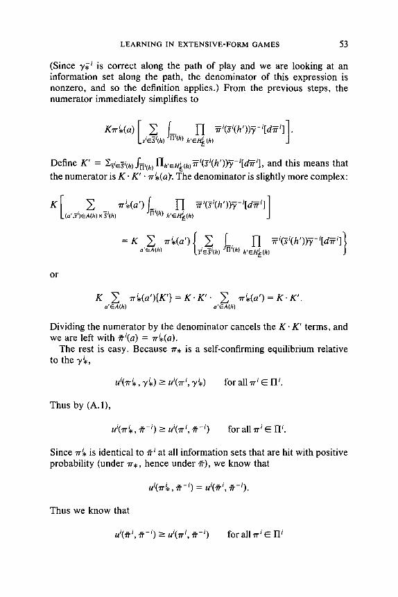
LEARNING IN EXTENSIVE-FORM GAMES 53
(Since yg" is correct along the path of play and we are looking at an information set along the path, the denominator of this expression is nonzero, and so the definition applies.) From the previous steps, the numerator immediately simplifies to
g'lTi~(a)[siE_~i~(hS-~i(h } 1-I ~ i ( - s i (h ' ) ) '~ - i [d~ i]] • h' el-lJ~ (h)
i --i . . -- i --i ~ - - - i i Define K' = E~ es (h) f~'cl0 I-Ih'eH~(hJ 7r (S (h))y [d-ff ], and this means that
the numerator is K" K' • ~r ~(aT. The denominator is slightly more complex:
I(a','g')~.A(I)x'Si h) "/r~(at) ('' l-I ~i(-gi(h'))7-i[dNi]] K ~ 3"~'(h) h'elt~(h)
= K 7r'*(a'){~ie?~(h S~;(h ) I-I ~i(-si(h'))~-i[d~i]} a'EA(h) h' EH~ (h)
o r
K ~ 7r~(a'){K'} = K'K" ~'~ 7r/,(a ') = K'K'. a'EA(h) a'EA(h)
Dividing the numerator by the denominator cancels the K . K' terms, and we are left with #i(a) = rri,(a).
The rest is easy. Because rr, is a self-confirming equilibrium relative to the y ' , ,
ui(~ i,, y i,) > ui(rr i, y i,) for all 7r i E H i.
Thus by (A.1),
ui(Ti.i~, ~T-i) ~ tli(,.rt.i, # - i ) f o r al l 7r i E 1-I i.
Since ~-~, is identical to #i at all information sets that are hit with positive probability (under rr , , hence under #), we know that
idi(,.i.t.i~, # - i ) = idi(#i, # - i ) .
Thus we know that
ui(~.fi, # - i ) ~ ui(,lr i, ~.f-i) f o r a l l ¢r i E H i

54
(and fo r i = profi le. •
FUDENBERG AND KREPS
1, 2), which means that ¢r is a N a s h equ i l ib r ium st ra tegy
ACKNOWLEDGMENTS
We are grateful to Robert Anderson, Robert Aumann, Ehud Kalai, David Levine, two referees, and the associate editor for helpful comments. We thank IDEI, Toulouse, and the Institute for Advanced Studies, Tel-Aviv University, for their hospitality while this research was being conducted. The financial assistance of the National Science Foundation (Grants SES 88-08204, SES 90-08770, SES 89-08402, and SES 92-08954) and the John Simon Guggen- heim Foundation is gratefully acknowledged.
REFERENCES
AUMANN, R. J. (1987). "Correlated Equilibrium as an Expression of Bayesian Rationality," Econometrica 55, 1-18.
BAT'nGALLI, P. (1987). "Comportamento razionale ed equilibrio nei giochi e nelle situazioni sociali," unpublished dissertation, Universitfi Commerciale L. Bocconi, Milano.
BATTIGALLI, P., AND GUAITOLI, P. (1988). "Conjectural Equilibrium," mimeo, Bocconi University.
BRANDENBURGER, A., AND DEKEL, E. (1987). "Rationalizability and Correlated Equilib- rium," Econometrica 55, 1391-1402.
ELLISON, G. (1993). "A Little Rationality and Learning from Personal Experience," mimeo, Harvard University.
FUDENBERG, D., AND KREPS, D. (1993). "Learning Mixed Equilibria," Games Econ. Behav. 5, 320-367.
FUDENBERG, D., AND KREPS, D. (1994). "Learning in Extensive-Form Games. II. Experi- mentation and Nash Equilibrium," mimeo, Stanford University.
FUDENaERG, D., AND LEVlNE, D. (1993a). "Self-Confirming Equilibrium," Econometrica 61, 523-546.
FUDENBERG, D., AND LEVINE, D. (1993b). "Steady State Learning and Nash Equilibrium," Econometrica 61, 547-574.
HAHN, F. (1977). "Exercises in Conjectural Equilibrium Analysis," Scand. J. Econ. 79, 210-226.
HARSANYI, J. C. (1973). "Games with Randomly Distrubed Payoffs: A New Rationale for Mixed-Strategy Equilibrium Points," Int. J. Game Theory 2, 1-23.
KALAI, E., AND LEHRER, E. (1993a). "Rational Learning Leads to Nash Equilibrium," Econometrica 61, 1019-1046.
KALAI, E., AND LEHRER, E. (1993b). "Subjective Equilibria in Repeated Games," Econo- metrica 61, 1231-1240.
KALAI, E., AND LEHRER, E. (1993c). "Subjective Games and Equilibria," mimeo, 1993. KOHLBERG, E., AND MERTENS, J.-F. (1986). "On the Strategic Stability of Equilibria,"
Econometrica 54, 1003-1037. KREPS, D. (1990). Game Theory and Economic Modelling. Oxford: Oxford Univ. Press.

LEARNING IN EXTENSIVE-FORM GAMES 55
KUHN, H. (1953). "Extensive games and the Problem of information," in Contributions to the Theory of Games, (H. Kuhn and A. Tucker, Eds.) Vol. 2, pp. 193-216, Princeton, NJ: Princeton Univ. Press.
RUB1NSTEIN, A., AND WOLINSKY, A. (1990). "Rationalizable Conjectural Equilibrium: Between Nash and Rationalizability," mimeo, Northwestern University.
SELTEN, R. (1975). "Reexamination of the Perfectness Concept for Equilibrium Points in Extensive Games," Int. J. Game Theory 4, 25-55.