using refinements of nash equilibria for solving extensive ... · these games are called two-player...

Czech Technical University in Prague

Faculty of Electrical Engineering

Department of Computer Science and Engineering

Master's Thesis

Using Re�nements of Nash Equilibria for SolvingExtensive-Form Games

Ji°í �ermák

Supervisor: Mgr. Branislav Bo²anský

Study Programme: Open informatics

Field of Study: Arti�cial Intelligence

May 12, 2014

vii

Aknowledgements

Here I would like to thank my supervisor Mgr. Branislav Bo²anský for his time and valuableassistance during the creation of this work. I would also like to thank my family and friendsfor their support.

Abstract

There is a growing number of applications of game theory in the real world, especially in eco-nomical and security domains. There are two main challenges brought by these applications.First challenge is created by the need of robust solutions, caused by the non-rational natureof the human opponents encountered in these applications. Second challenge lies in the sizeof the games which need to be solved. This thesis addresses both of these issues. It provides�rst thorough experimental evaluation of existing advanced solution concepts on a set ofreal world inspired games. The best solution concept is then applied to the Double oraclealgorithm, which is one of the most suitable algorithms for solving large domains found inthese applications. The aim of this action is to even further increase the performance ofthis algorithm, by exploiting higher quality of solutions provided by the advanced solutionconcept.

Abstrakt

Existuje stále rostoucí mnoºství aplikací teorie her ve scéná°ích ze skute£ného sv¥ta, hlavn¥v bezpe£nostních a ekonomický doménách. Tyto aplikace p°iná²í dv¥ výzvy. První výzva jetvo°ena pot°ebou robustn¥j²ích °e²ení, zp·sobenou neracionální povahou lidských protivník·vyskytujících se v t¥chto aplikacích. Druhá výzva je tvo°ená velikostí her, které je pot°eba°e²it. Tato práce pomáhá °e²it oba tyto problémy. Poskytuje první experimentální ohod-nocení existujících pokro£ilých koncept· °e²ení na mnoºin¥ her, inspirovaných skute£nýmsv¥tem. Nejlep²í z t¥chto °e²ení je pak aplikováno do Double oracle algoritmu, coº je je-den z nejvhodn¥j²ích algoritm· pro °e²ení rozsáhlých domén, se kterými se setkáváme vt¥chto aplikacích. Cílem této akce je zvý²ení jeho výkonu, pomocí vyuºití kvalitn¥j²ích°e²ení poskytnutých tímto konceptem.

xi

Contents

1 Introduction 1

1.1 Thesis outline . . . . . . . . . . . . . . . . . . . . . . . . . . . . . . . . . . . . 2

2 Introduction to Game Theory 3

2.1 Normal-form Games . . . . . . . . . . . . . . . . . . . . . . . . . . . . . . . . 32.2 Extensive-form Games . . . . . . . . . . . . . . . . . . . . . . . . . . . . . . . 4

3 Nash Equilibrium and Re�nements 7

3.1 Nash equilibrium . . . . . . . . . . . . . . . . . . . . . . . . . . . . . . . . . . 73.2 Re�nements in Normal-form Games . . . . . . . . . . . . . . . . . . . . . . . 7

3.2.1 Undominated equilibrium . . . . . . . . . . . . . . . . . . . . . . . . . 83.2.2 Perfect equilibrium . . . . . . . . . . . . . . . . . . . . . . . . . . . . . 83.2.3 Proper equilibrium . . . . . . . . . . . . . . . . . . . . . . . . . . . . . 10

3.3 Re�nements in Extensive-form Games . . . . . . . . . . . . . . . . . . . . . . 103.3.1 Subgame perfect equilibrium . . . . . . . . . . . . . . . . . . . . . . . 113.3.2 Undominated equilibrium . . . . . . . . . . . . . . . . . . . . . . . . . 123.3.3 Sequential equilibrium . . . . . . . . . . . . . . . . . . . . . . . . . . . 123.3.4 Quasi-perfect equilibrium . . . . . . . . . . . . . . . . . . . . . . . . . 133.3.5 Normal-form proper equilibrium . . . . . . . . . . . . . . . . . . . . . 143.3.6 Perfect equilibrium . . . . . . . . . . . . . . . . . . . . . . . . . . . . . 153.3.7 Proper equilibrium . . . . . . . . . . . . . . . . . . . . . . . . . . . . . 15

4 Algorithms for computing Nash equilibrium re�nements 19

4.1 Nash equilibrium . . . . . . . . . . . . . . . . . . . . . . . . . . . . . . . . . . 194.2 Undominated equilibrium . . . . . . . . . . . . . . . . . . . . . . . . . . . . . 214.3 Quasi-perfect equilibrium . . . . . . . . . . . . . . . . . . . . . . . . . . . . . 214.4 Normal-form proper equilibrium . . . . . . . . . . . . . . . . . . . . . . . . . . 23

5 Re�nement Comparison 27

5.1 Imperfect Opponents . . . . . . . . . . . . . . . . . . . . . . . . . . . . . . . . 275.1.1 Counter-factual regret minimization . . . . . . . . . . . . . . . . . . . 275.1.2 Monte-Carlo tree search . . . . . . . . . . . . . . . . . . . . . . . . . . 285.1.3 Quantal-response equilibrium . . . . . . . . . . . . . . . . . . . . . . . 29

5.2 Experimental domains . . . . . . . . . . . . . . . . . . . . . . . . . . . . . . . 295.2.1 Leduc holdem poker . . . . . . . . . . . . . . . . . . . . . . . . . . . . 305.2.2 Goofspiel . . . . . . . . . . . . . . . . . . . . . . . . . . . . . . . . . . 30

xiii

xiv CONTENTS

5.2.2.1 Imperfect-information Goofspiel . . . . . . . . . . . . . . . . 305.2.3 Random games . . . . . . . . . . . . . . . . . . . . . . . . . . . . . . . 30

5.3 Experimental Settings . . . . . . . . . . . . . . . . . . . . . . . . . . . . . . . 325.4 Results . . . . . . . . . . . . . . . . . . . . . . . . . . . . . . . . . . . . . . . . 32

6 Double-oracle algorithm 35

6.1 Restricted game . . . . . . . . . . . . . . . . . . . . . . . . . . . . . . . . . . . 356.1.1 Inconsistencies in the restricted game . . . . . . . . . . . . . . . . . . . 35

6.2 Best response algorithm . . . . . . . . . . . . . . . . . . . . . . . . . . . . . . 366.2.1 Nodes of the other players . . . . . . . . . . . . . . . . . . . . . . . . . 376.2.2 Nodes of the searching player . . . . . . . . . . . . . . . . . . . . . . . 38

6.3 Player selection . . . . . . . . . . . . . . . . . . . . . . . . . . . . . . . . . . . 396.4 Termination . . . . . . . . . . . . . . . . . . . . . . . . . . . . . . . . . . . . . 396.5 Main loop . . . . . . . . . . . . . . . . . . . . . . . . . . . . . . . . . . . . . . 396.6 Re�nements in Double oracle . . . . . . . . . . . . . . . . . . . . . . . . . . . 39

7 Results 41

7.1 Experimental domains . . . . . . . . . . . . . . . . . . . . . . . . . . . . . . . 417.1.1 Border patrol . . . . . . . . . . . . . . . . . . . . . . . . . . . . . . . . 417.1.2 Generic poker . . . . . . . . . . . . . . . . . . . . . . . . . . . . . . . . 42

7.2 Experimental setting . . . . . . . . . . . . . . . . . . . . . . . . . . . . . . . . 427.3 Results . . . . . . . . . . . . . . . . . . . . . . . . . . . . . . . . . . . . . . . . 437.4 Theoretical analysis . . . . . . . . . . . . . . . . . . . . . . . . . . . . . . . . 45

8 Conclusion 47

8.1 Future work . . . . . . . . . . . . . . . . . . . . . . . . . . . . . . . . . . . . . 48

A CD Content 49

A.1 Game theoretical library . . . . . . . . . . . . . . . . . . . . . . . . . . . . . . 49A.2 Parameters of experiments . . . . . . . . . . . . . . . . . . . . . . . . . . . . . 49

A.2.1 Re�nement comparison experiment parameters . . . . . . . . . . . . . 49A.2.2 Double oracle performance experiment parameters . . . . . . . . . . . 50

List of Figures

2.1 Prisoner's Dilemma as an extensive-form game . . . . . . . . . . . . . . . . . 5

3.1 (a) A game where player 1 needs to consider mistake in the future of player2. (b) A game where player 2 needs to consider mistake in the past. . . . . . 11

3.2 A game with no subgame . . . . . . . . . . . . . . . . . . . . . . . . . . . . . 123.3 Matching Pennies on Christmas Morning [10] . . . . . . . . . . . . . . . . . . 143.4 A game with unique perfect equilibrium . . . . . . . . . . . . . . . . . . . . . 153.5 (a) The game where properness rules out all insensible equilibria (b) The game

where normal-form properness rules out all insensible equilibria. . . . . . . . . 163.6 (a) The relations between re�nements in two-player zero-sum extensive-form

games. (b) The relations between re�nements in normal-form games. . . . . . 16

4.1 Matching Pennies on Christmas Morning [10] . . . . . . . . . . . . . . . . . . 19

5.1 Overview of the utility value for di�erent equilibrium strategies. . . . . . . . . 315.2 Overview of the relative utility value for di�erent equilibrium strategies. . . . 33

6.1 A demonstration of inconsistencies in the restricted game . . . . . . . . . . . 36

7.1 (a) Border patrol on a connected grid (b) Border patrol on a partially con-nected grid . . . . . . . . . . . . . . . . . . . . . . . . . . . . . . . . . . . . . 41

7.2 Overview of results of Double oracle algorithm on Generic poker . . . . . . . 427.3 Overview of results of Double oracle algorithm on Goofspiel . . . . . . . . . . 437.4 Overview of results of Double oracle algorithm on Border patrol . . . . . . . . 447.5 Time spend solving LPs during the Double oracle computation . . . . . . . . 457.6 Domain for demonstration of Double oracle with di�erent solvers . . . . . . . 46

xv

xvi LIST OF FIGURES

List of Tables

2.1 Prisoner's Dilemma as a normal-form game . . . . . . . . . . . . . . . . . . . 4

3.1 Normal-form game with a non-robust equilibrium . . . . . . . . . . . . . . . . 83.2 Normal-form game with two perfect equilibria . . . . . . . . . . . . . . . . . . 93.3 Proper equilibrium in�uenced by adding strictly dominated strategy . . . . . 10

xvii

xviii LIST OF TABLES

Chapter 1

Introduction

Game theory is a widely used approach for analysing multi-agent interaction using mathe-matical models, with an aim to �nd a behavior optimizing rewards obtained by players. Inthe recent years a growing number of real world applications of game theoretical approachesemerged, including placement of security checkpoints around airports [13], scheduling ofFederal air marshals to commercial �ights [19], development of poker players on the level ofprofessional human players [15] or trading agents in auctions [24].

The main aim of game theory is to �nd the optimal behavior in various scenarios calledgames. Such a behavior is called strategy and is prescribed by a solution concept. The mostfamous and widely used solution concept is the Nash equilibrium [12], which is guaranteed toprescribe the optimal behavior to every player in the game, under the assumption of rationalopponents. The main shortcoming of this solution concept is that it doesn't exploit mistakesmade. So for example if in the game of poker one player by accident creates an opportunityfor the second player to win 1000$ instead of the expected win of 1$ it is consistent with Nashequilibrium to ignore this opportunity and proceed to win the expected 1$ prize. This iscaused by the fact that Nash equilibrium expects fully rational player and so it assumes thatsuch mistake will never happen. This is a serious issue since such mistakes are common in thereal world applications. This is caused by the fact that the opponents in these applicationsare usually humans, which are known to behave irrationally in various scenarios.

There is a number of solution concepts called re�nements of the Nash equilibrium whichattempt to cope with these issues. These concepts still guarantee the optimality againstrational opponents and further improve the Nash equilibrium, exploiting various types ofmistakes of the opponents or even by the player himself. And so when one encounters anunexpected situation, where there is a pro�t higher then expected achievable, these solutionconcepts should prescribe behavior maximizing the pro�t. Unfortunately, the only compar-ison of existing re�nements available, is performed on small, arti�cially created domains,speci�cally tailored to show some desirable property. In the �rst part of this thesis we will�ll this gap for a two player games with sequential interaction in fully competitive environ-ment, with imperfect information caused by unobservable actions of opponents or stochasticenvironment. These games are called two-player zero-sum extensive-form games with imper-fect information. We provide experimental evaluation of chosen re�nements on real worldinspired two-player zero-sum extensive-form games, such as card games or border patrolling

1

2 CHAPTER 1. INTRODUCTION

scenarios. Their overall performance is discussed along with implementational complications,such as numerical stability, which need to be overcome in order to compute them.

Furthermore thanks to the demand of scalability introduced by often large applications,several algorithms speci�cally created to solve large extensive-form games emerged. Thesealgorithms allow further deployment of the game theoretical approaches to various, previ-ously too complex, domains. For example, there is the Counterfactual regret minimizationalgorithm [25] which was successful in solving poker games orders of magnitude larger thanthe current state of the art. Another of such algorithms is the Double oracle algorithm [1]which solves large games by iteratively building a smaller game, computing its Nash equi-librium. This procedure is repeated until the solution of this smaller game equals to thesolution of the complete game. This approach o�ers a possibility to solve games faster, whilealso saving the memory needed, since there is no need to construct the whole representationof the original game.

The main topic of this thesis is the incorporation of the best suitable re�nement to theDouble oracle algorithm to further improve its performance, by computing more sensiblestrategies in every iteration.

1.1 Thesis outline

Chapter 2 provides a brief introduction of the most used representations of games. Chapter3 de�nes the Nash equilibrium and the most known re�nements. Chapter 4 contains adiscussion about the computational aspects of previously de�ned re�nements. Chapter 5is based on �ermák et al. [26] and presents results of comparison of re�nements of Nashequilibrium. Chapter 6 formally introduces the Double oracle algorithm. Chapter 7 presentsresults of Double oracle algorithm using re�ned solver. Chapter 8 contains a conclusion ofthe thesis.

Chapter 2

Introduction to Game Theory

This chapter presents the most known representations of the games. We provide the descrip-tion and formal de�nitions of normal-form and extensive-form games. The main focus ofthis thesis is on two-player zero-sum extensive-form games with imperfect information andperfect recall, however number of concepts discussed in following chapters make use of thenormal-form representation and so this representation was not omitted. Furthermore everyextensive-form game can be converted to the normal-form representation, and so this repre-sentation should be thoroughly analyzed. Even though it may appear that the limitationsused are too restrictive, they still permit a large number of purely competitive scenarios,where the gain of one player equals to the loss of the other. In addition, they allow the pos-sibility of unobservable moves of the opponent or the stochastic environment, dramaticallyincreasing the number of domains consistent with such representation. The restriction toperfect recall means that every player remembers what he did in the past along with all theinformations he obtained during the play. Between games consistent with these restrictionbelong classical games such as chess, two player poker or more realistic scenarios such assecurity of industrial objects.

2.1 Normal-form Games

Normal-form games typically represent one-shot simultaneous moves games, using a matrix,assigning utility value for every combination of actions of players. This representation doesn'texploit any structure, such as sequential interaction between players, of the game played.Instead it simply evaluates every pair of actions, under assumption that both players playsimultaneously. These facts make normal-form unsuitable for representation of larger games.

De�nition 1. Two player normal-form game is a tuple (P, A, u) where:

1. P is a set of 2 players indexed by i

2. A = A1 ×A2 where Ai is a �nite set of actions available to player i

3. u = (u1, u2) where ui : A → R is a utility function for player i

3

4 CHAPTER 2. INTRODUCTION TO GAME THEORY

C ′ D′

C -1, -1 -4, 0D 0, -4 -3, -3

Table 2.1: Prisoner's Dilemma as a normal-form game

As an example of the normal-form game consider the game called Prisoner's Dilemmadepicted in Table 2.1. Prisoner's Dilemma describes a scenario where two prisoners sit underinterrogation in di�erent rooms. Both of them have the possibility to cooperate (with theother prisoner) C or to defect D. Both players act simultaneously, which means that neitherof them knows what the other did when deciding. The utility matrix in Table 2.1 describesthe outcomes for every combination of all available actions.

Let us now discuss strategies of players. A strategy can be seen as a plan prescribingbehavior to a player. A set of pure strategies Si corresponds to the set of actions Ai. A setof mixed strategies ∆i contains all the probability distributions δi over the set Si. A strategypro�le is a vector of strategies, one for each player.

2.2 Extensive-form Games

Extensive-form games provide a representation which is more suitable for description of sce-narios which evolve in time. This representation allows every player to choose action in eachstate of the game, using exponentially smaller representations in the form of a game treeinstead of the utility matrix. Nodes of this tree represent the states of the game and edgesactions available in the corresponding states. Leafs represent the terminal states and havethe utility value for all players associated with them, representing their preference of thisoutcome. We distinguish two types of extensive-form games, perfect-information and imper-fect information ones. In perfect-information games every player knows everything aboutthe state of the game, whilst in imperfect-information games some of these informations maybe hidden.

De�nition 2. A �nite extensive-form game with perfect information has the following com-

ponents:

1. A �nite set P of players

2. A �nite set H of sequences, the possible histories of actions, such that the empty se-

quence is in H and every pre�x of a sequence in H is also in H. Z ⊆ H are the terminal

histories (those which are not a pre�x of any other sequences). A(h) = {a : (h, a) ∈ H}are the actions available after a nonterminal history h ∈ H.

3. A function P (h) that assigns to each nonterminal history (each member of H\Z) a

member of P ∪ {c}. P (h) is the player who takes an action after the history h. If

P (h) = c then chance determines the action taken after history h.

2.2. EXTENSIVE-FORM GAMES 5

4. A function fc that associates with every history h for which P (h) = c a probability

measure fc(.|h) on A(h) (fc(a|h) is the probability that a occurs given h), where each

such probability measure is independent of every other such measure.

5. For each player i ∈ P a utility function ui from terminal states Z to R. If P = {1, 2}and u2 = −u1 it is a zero sum extensive-form game.

De�nition 3. A �nite extensive-form game with imperfect information is a tuple (P,H, P, fc, I, u),with following components:

1. Perfect-information extensive-form game (P,H, P, fc, u)

2. For each player i ∈ P a partition Ii of {h ∈ H : P (h) = i} with the property that

A(h) = A(h′) whenever h and h' are in the same member of the partition. For Ii ∈ Iiwe denote by A(Ii) the set A(h) and by P (Ii) the player P (h) for any h ∈ Ii. Ii is theinformation partition of player i; a set Ii ∈ Ii is an information set of player i

Informally, every information set Ii for player i contains all game states h which areindistinguishable for i.

Figure 2.1: Prisoner's Dilemma as an extensive-form game

As an example consider the imperfect-information extensive-form game from Figure 2.1.It is again the Prisoner's Dilemma, this time represented as an extensive-form game. Player1 plays �rst and makes a choice in the root of the game tree. As we can see the states afterboth choices are grouped into 1 information set, because they are indistinguishable for player2. The leaf of the tree and therefore terminal state of the game is reached after the actionof player 2 and the outcome of the game is evaluated.

Next we provide the formal de�nition of perfect recall, which is one of the propertiesrequired from the games used in this thesis.

De�nition 4. Player i has a perfect recall in an imperfect-information game G if for any two

nodes h, h′, that are in the same information set Ii, for any path h0, a0, h1, a1, h2, ..., hm, am, hfrom the root of the game to h (where the hj are decision nodes and the aj are actions) and

for any path h0, a′0, h′1, a′1, h′2, ..., h

′m′ , a

′m′ , h

′ from the root to h′ it must be the case that:

6 CHAPTER 2. INTRODUCTION TO GAME THEORY

1. m = m′

2. for all 0 ≤ j ≤ m, if P (hj) = i (i.e., hj is a decision node of player i), then hj and h′j

are in the same equivalence class for i;

3. for all 0 ≤ j ≤ m, if P (hj) = i (i.e., hj is a decision node of player i), then aj = a′j.

Let us now discuss strategies in extensive-form games. A pure strategy for player i isa mapping Ii → A(Ii). Si is a set of all pure strategies for player i. A mixed strategy δiis again a probability distribution over elements of Si, with ∆i representing the set of allmixed strategies for i. In the extensive form games, we can represent strategies as behavioralstrategies bi, which assign probability distribution over A(Ii),∀Ii ∈ Ii. For all games withperfect recall, behavioral strategies have the same expressive power as mixed strategies [6].

Finally in the games of perfect recall, we can use sequence-form representation [4]. Asequence σi is a list of actions of player i ordered by their occurrence on the path from theroot of the game tree to some node. These sequences are used to represent the strategy as arealization plan ri. The realization plan ri assigns the probability to sequences σi of playeri, assuming other players play such that the actions of σi can by executed. Furthermore risatis�es the network �ow property, i.e. ri(σ) =

∑a∈A(I) ri(σ · a), where I is an information

set reached by sequence σ and σ · a stands for σ extended by action a.

Thanks to the equality of strategy representations above, we overload the notation ofutility function to u(si, s−i) as the utility of the state reached when playing according to siand s−i, u(δi, δ−i) as an expected utility, when playing according to δi and δ−i and similarlyu(bi, b−i) and u(ri, r−i). Furthermore let us denote Ui(si|∆) as the utility obtained wheni plays si and the rest of the players follows strategy pro�le ∆. Ui(I, a|B) is the utilityobtained by i in information set I, when playing action a in I and according to strategypro�le B otherwise.

This chapter provided description of the types of games and restrictions we will assumethrough this thesis. The next chapter will use this background to describe various solutionconcepts used for solving normal-form and extensive-form games.

Chapter 3

Nash Equilibrium and Re�nements

This chapter introduces optimal strategies for games described by solution concepts. Themost famous solution concept of Nash equilibrium is introduced and all its shortcomingsdiscussed. Next we describer the most known re�nements of the Nash equilibrium for bothnormal-form and extensive-form games.

3.1 Nash equilibrium

Nash equilibrium is a solution concept due to Nash [12], which prescribes the optimal be-havior under the assumption of opponents playing to maximize their outcome. Let us �rstde�ne the notion of the best response.

De�nition 5. Strategy δ∗i is the best response to strategy δ−i i� u(δ∗i , δ−i) ≥ u(δi, δ−i), ∀δi ∈∆i. We denote br(δi) as the set of all best responses to δi.

Informally the Nash equilibrium is such a strategy pro�le where no player wants todeviate from its strategy, even when he learns the strategy of others. Note that there mightbe an in�nite number of such strategy pro�les. A player doesn't want to deviate from hisstrategy only when he plays according to the best response to strategies of all other players,and so we arrive to the formal de�nition of Nash equilibrium.

De�nition 6. Strategy pro�le ∆ is a Nash equilibrium i� ∀δi ∈ ∆ : δi ∈ br(δ−i).

As an example lets consider the game from Table 3.1. There are two Nash equilibriain the example, namely (α1, α2) and (β1, β2). Since br(α1) = {α2} and br(α2) = {α1},(α1, α2) is indeed Nash equilibrium. Same goes for (β1, β2), since br(β1) = {α2, β2} andbr(β2) = {α1, β1}.

3.2 Re�nements in Normal-form Games

The need to re�ne Nash equilibrium strategies in normal-form games follows from the factthat the Nash equilibrium doesn't exploit possible mistakes of the opponent. Let us considerthe game in Table 3.1. As shown above, this game has two Nash equilibria (α1, α2) and

7

8 CHAPTER 3. NASH EQUILIBRIUM AND REFINEMENTS

(β1, β2) since in both cases there is no gain for either of the players obtained by deviatingfrom given strategy pro�le. However, thanks to the structure of this particular game, neitherof them can actually lose anything by changing strategy from βi to αi. There is only oneequilibrium optimal when considering possible mistakes of the opponent (α1, α2). Solutionconcepts introduced in this section will attempt to preserve only the rational equilibria.

α2 β2α1 1, 1 0, 0β1 0, 0 0, 0

Table 3.1: Normal-form game with a non-robust equilibrium

3.2.1 Undominated equilibrium

The main idea behind this equilibrium is, that if choosing between two actions, where oneof them is at least as good as the other no matter what the opponent does and better for atleast one action of the opponent, one should always prefer this action over the other. Thisrelation between actions is called weak dominance. Formally strategy s1i weakly dominatess2i i� ∀s−i ∈ S−i : u(s1i , s−i) ≥ u(s2i , s−i) and ∃s−i ∈ S−i : u(s1i , s−i) > u(s2i , s−i). And so theundominated equilibrium in normal-form games is such a Nash equilibrium which consistsonly of those strategies, which are not weakly dominated by any other strategy.

The only undominated equilibrium of the game from Figure 3.1 is (α1, α2), because αidominates βi, ∀i ∈ P. In the game from Figure 3.2, which was created from the game inTable 3.1 by adding actions γ1 and γ2, are two undominated equilibria, namely (α1, α2) and(β1, β2), because the only dominated actions of this game are γ1 and γ2, and so the onlyNash equilibrium which is not undominated is (γ1, γ2).

3.2.2 Perfect equilibrium

Solution concept due to Selten et al. [16]. The basic idea behind this concept is, that itis possible for every player to make mistakes with a small probability. And so every playerneeds to consider all the outcomes of his actions, not only the ones expected when consideringrational opponent. Let us �rst de�ne ε-perfect equilibrium.

De�nition 7. An ε-perfect equilibrium is a fully mixed strategy pro�le ∆ = (δ1, ..., δn) such

that

Uj(sj |∆) < Uj(s′j |∆)⇒ δj(sj) ≤ ε, ∀j ∈ P,∀sj , s′j ∈ Sj (3.1)

A perfect equilibrium is then de�ned as the limit of ε-perfect equilibria. That is (δ1, ..., δn)is a perfect equilibrium i� there exists sequence {ε}∞k=1 and (δk1 , ..., δ

kn)∞k=1 such that each

εk > 0 and limk→∞

εk = 0, each (δk1 , ..., δkn) is an εk-perfect equilibrium and lim

k→∞δki (si) =

δi(si),∀i ∈ P,∀si ∈ Si.

3.2. REFINEMENTS IN NORMAL-FORM GAMES 9

For any game in normal form, the perfect equilibria form a non-empty subset of Nashequilibria [16]. Furthermore every perfect equilibrium is undominated and for two-playerzero-sum games every undominated equilibrium is perfect [22].

Let us now examine perfect equilibria of our motivational game from Table 3.1. Considerfollowing strategy pro�le.

δε1(α1) = ε, δε1(β1) = 1− ε (3.2)

δε2(α2) = ε, δε2(β2) = 1− ε (3.3)

Responses for this pro�le and player 1 are then evaluated.

U1(α1|δε1, δε2) = ε (3.4)

U1(β1|δε1, δε2) = 0 (3.5)

As we can see, the best response here is α1 and so this pro�le is not ε-perfect equilibrium.From the fact that there is only one Nash equilibrium left and the set of perfect equilibria isalways non-empty follows that (α1, α2) is perfect equilibrium.

α2 β2 γ2α1 1, 1 0, 0 -9, -9β1 0, 0 0, 0 -7, -7γ1 -9, -9 -7, -7 -7, -7

Table 3.2: Normal-form game with two perfect equilibria

Now let us examine the game represented in normal form in Table 3.2, which was createdfrom the game in Table 3.1 by adding actions γ1 and γ2. The outcome we would like toachieve once again is (α1, α2), since both added actions are dominated. And indeed thisstrategy pro�le is still Nash equilibrium. There are however two additional pure strategyNash equilibria, namely (β1, β2) and (γ1, γ2). Of these only (γ1, γ2) is not perfect. Let usnow show that (β1, β2) is perfect equilibrium. We choose following strategy pro�le.

δε1(α1) = ε, δε1(β1) = 1− 2ε, δε1(γ1) = ε (3.6)

δε2(α2) = ε, δε2(β2) = 1− 2ε, δε2(γ2) = ε (3.7)

Responses for this pro�le and player 1 are then evaluated as follows.

U1(α1|δε1, δε2) = −8ε (3.8)

U1(β1|δε1, δε2) = −7ε (3.9)

U1(γ1|δε1, δε2) = −7− 2ε (3.10)

So β1 is the best response to δε2 and as required in (3.1) δε1(α1) ≤ ε, δε1(γ1) ≤ ε. Then as εconverges to zero (δε1, δ

ε2) converge to the strategies which select β1 and β2 with probability

1, implying that (β1, β2) is indeed perfect equilibrium. This property is caused by addingdominated strategies (γ1, γ2) to the game and was pointed out by Myerson et al. [11].


α3 β3α2 β2

α1 1, 1, 1 0, 0, 1β1 0, 0, 1 0, 0, 1

α2 β2α1 0, 0, 0 0, 0, 0β1 0, 0, 0 1, 1, 0

Table 3.3: Proper equilibrium in�uenced by adding strictly dominated strategy

3.2.3 Proper equilibrium

Solution concept due to Myerson et al.[11], which is robust against small perturbations instrategies. These perturbations have some additional properties added with an aim to resolvethe issues mentioned in previous section. They are considered to be rational, meaning thatthe costly mistake is expected with an order of magnitude smaller probability than the cheapone. Let us �rst de�ne ε-proper equilibria.

De�nition 8. ε-proper equilibrium is a fully mixed strategy pro�le ∆ = (δ1, ..., δn) such that

Uj(sj |∆) < Uj(s′j |∆)⇒ δj(sj) ≤ ε · δj(s′j), ∀j ∈ P,∀sj , s′j ∈ Sj (3.11)

This de�nition directly implies that every ε-proper equilibrium is ε-perfect since δj(sj) ≤ε · δj(s′j)⇒ δj(sj) ≤ ε, ∀j ∈ P, ∀sj , s′j ∈ Sj but the opposite doesn't hold. Strategy pro�le(δ1, ..., δn) is a proper equilibrium i� there exist some sequences {ε}∞k=1 and (δk1 , ..., δ

kn)∞k=1

such that each εk > 0 and limk→∞

εk = 0, each (δk1 , ..., δkn) is εk-proper equilibrium and

limk→∞

δki (si) = δi(si), ∀i ∈ P,∀si ∈ Si. For any game in normal form, the proper equilib-

ria form a non-empty subset of perfect equilibria [11]Now let us return to the game from Table 3.2. Let us check that the strategy pro�le from

(3.6) and (3.7) is not ε-proper equilibrium. Since for 0 < ε < 1 holds that U1(γ1|δε1, δε2) <U1(α1|δε1, δε2) but from δ1(γ1) > ε ·δ1(α1) follows that (β1, β2) is not ε-proper equilibrium. Aswe can see insisting on properness removed the undesirable property of perfect equilibrium,by expecting more costly mistakes to have much smaller probability of occurrence than theless costly ones.

However to show that this issue is not fully resolved by the proper equilibrium let usdiscuss a 3 player game shown in Table 3.3 taken from [22]. If we limit third players actiononly to α3 (left table) then (α1, α2, α3) is an unique proper equilibrium of this game. Howeverby adding second action β3 for third player, which is strictly dominated, we create anotherproper equilibrium (β1, β2, α3), and so we see that even though proper equilibrium �xes thisissue in some games, there are still examples where the undesirable equilibria get picked.

3.3 Re�nements in Extensive-form Games

The main shortcoming of Nash equilibrium in extensive-form games is, that it guaranteesrational behavior only when the rest of the players play rationally, with no concern for gainspossibly caused by mistakes of said opponents. We distinguish two types of mistakes againstwhich one would like to be optimal. The �rst type is called mistakes in the past. When this

3.3. REFINEMENTS IN EXTENSIVE-FORM GAMES 11

Figure 3.1: (a) A game where player 1 needs to consider mistake in the future of player 2.(b) A game where player 2 needs to consider mistake in the past.

mistake occurs a player �nds himself in the part of the tree, which he didn't expect to visit,when considering rational opponent. As an example consider the game from Figure 3.1(b).In this game, there is no motivation for player 2 to prefer R over L, since he expects player1 to always choose U immediately ending the game. The second type of mistakes is calledmistakes in the future. To be optimal against this type of mistakes, player i should pushhis opponent to situations, where he needs to choose between for him bad and good actions.The opponent then �nds himself in situations where the potential mistakes are as costly aspossible. As an example consider the game from Figure 3.1(a). Here player 1 should alwaysprefer D to U since he can only gain by playing D if player 2 makes a mistake by playingL. Following solution concepts will attempt to exploit these types of mistakes.

3.3.1 Subgame perfect equilibrium

Solution concept due to Kuhn [6]. Strategy pro�le B of game G is a subgame perfectequilibrium, if for every subgame G′ of G holds that B prescribes behavior consistent withNash equilibrium of G′. A subgame is a subset of the original game with following properties.(1) the root of the subgame is not in the information set with any other game state of theoriginal game. (2) if a game state belongs to the subgame, all its successors must also belongto the subgame. (3) if a game state belongs to the subgame, all the nodes contained in thesame information set must be also included in the subgame. Set of the subgame perfectequilibria forms a non-empty subset of Nash equilibria [6].

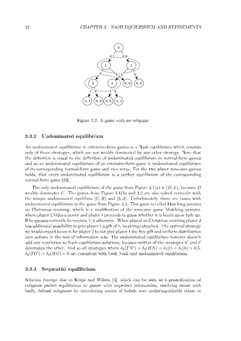
If we try this approach to our motivational game in Figure 3.1(b), we indeed see thatthe only subgame perfect equilibrium is (U,R), since playing L would violate equilibrium insubgame after action D of player 1. This is not a coincidence, since when the subgames arewell de�ned subgame perfect equilibium generates strategies optimal against the mistakesin the past. In the game from Figure 3.1(a) there are two subgame perfect equilibria (U,L)and (D,R) because optimality in subgames cannot exploit mistakes in the future. Thereare further issues with subgame perfection. For example let us consider the game in Figure3.2. As we can easily see, this game has no subgames (except for the game itself), since theinitial action of chance is unobservable for both players and so subgame perfect equilibriumdoesn't add any more restrictions to Nash equilibrium.


Figure 3.2: A game with no subgame

3.3.2 Undominated equilibrium

An undominated equilibrium in extensive-form games is a Nash equilibrium which consistsonly of those strategies, which are not weakly dominated by any other strategy. Note thatthe de�nition is equal to the de�nition of undominated equilibrium in normal-form gamesand so an undominated equilibrium of an extensive-form game is undominated equilibriumof its corresponding normal-form game and vice versa. For the two player zero-sum gamesholds, that every undominated equilibrium is a perfect equilibrium of the correspondingnormal-form game [22].

The only undominated equilibrium of the game from Figure 3.1(a) is (D,L), because Dweakly dominates U . The games from Figure 3.1(b) and 3.2 are also solved correctly withthe unique undominated equilibria (U,R) and (b, d). Unfortunately, there are issues withundominated equilibrium in the game from Figure 3.3. This game is called Matching pennieson Christmas morning, which is a modi�cation of the zero-sum game Matching pennies,where player 2 hides a penny and player 1 proceeds to guess whether it is heads up or tails up.If he guesses correctly he receives 1, 0 otherwise. When played on Christmas morning player 2has additional possibility to give player 1 a gift of 1, no strings attached. The optimal strategywe would expect to see is for player 2 to not give player 1 the free gift and uniform distributionover actions in the rest of information sets. The undominated equilibrium however doesn'tadd any restriction to Nash equilibrium solutions, because neither of the strategies h′ and t′

dominates the other. And so all strategies where δ2(TN ′) = δ2(HN) = δ1(t) = δ1(h) = 0.5,δ2(TG

′) = δ2(HG) = 0 are consistent with both Nash and undominated equilibrium.

3.3.3 Sequential equilibrium

Solution concept due to Kreps and Wilson [5], which can be seen as a generalization ofsubgame perfect equilibrium to games with imperfect information, resolving issues withbadly de�ned subgames by introducing notion of beliefs over undistinguishable states in


information sets. Insisting on sequentiality rules out equilibria not optimal against themistakes of the opponent in the past. Let us �rst de�ne two notions.

De�nition 9. A system of beliefs is a mapping µ

µ : S(I)→ [0, 1], ∀I ∈ I (3.12)

where S(I) is set of all states contained in information set I. It must hold that

∀I :∑s∈S(I)

µ(s) = 1 (3.13)

Less formally, the system of beliefs is player's assumption about the real state of thegame, given an information set.

De�nition 10. An assessment is a pair (µ,B), where µ is system of beliefs and B is a

behavioral strategy pro�le.

De�nition 11. An assessment (µ,B) is consistent if there exists sequence {µε, Bε}ε↓0 whereBε is completely mixed behavior strategy pro�le and µε is a system of beliefs generated by

Bε, such that

limε→0

(µε, Bε) = (µ,B) (3.14)

Sequential equilibrium is an assessment (µ,B) which is consistent and for which B issequential best response against (µ,B). Every sequential equilibrium is subgame perfectand is guaranteed to exist [5]. One of the positive properties of sequential equilibrium is,that it exploits mistakes made by opponent in the past. It doesn't however exploit possiblemistakes in the future. So for the game from Figure 3.1(a) there are again two sequentialequilibria (U,L) and (D,L) because the introduction of beliefs doesn't in any way help withthe mistakes in the future. The game from Figure 3.1(b) has only one sequential equilibriumbecause it further re�nes subgame perfection. Furthermore thanks to the beliefs the onlysequential equilibrium of the game from Figure 3.2 is the only rational one (b, d).

3.3.4 Quasi-perfect equilibrium

Informally solution concept due to van Damme [21] that requires each player at every infor-mation set to take a choice optimal against mistakes of the opponent.

De�nition 12. Fix an information set Ii. Let i be player which makes decision in Ii. An

Ii-local puri�cation of behavioral strategy bi is a behavioral strategy for i created by replacing

the behavior of i in Ii and every information set of i encountered after Ii, by behavior that

puts all probability mass on single action in these sets.

As an example consider the behvioral strategy in the game from Figure 3.3 b2(T ) = 1,b2(N

′) = b2(G′) = 0.5. There are two local puri�cations of the information set reached by

the action T , namely b2(T ) = b2(N′) = 1 and b2(T ) = b2(G

′) = 1.

De�nition 13. We say that an Ii-local puri�cation is an Ii-local best response to b−i if itachieves the best expected payo� among all Ii-local puri�cations.


Figure 3.3: Matching Pennies on Christmas Morning [10]

De�nition 14. Ii-local puri�cation b′i is ε-consistent with bi, if bi assigns behavioral proba-

bility strictly bigger than ε to the actions to which b′i assigns 1 in Ii and following information

sets of player i.

Strategy pro�le B is ε-quasi perfect if it is fully mixed and if for each player i and everyinformation set Ii belonging to i, all Ii-local puri�cations of bi that are ε-consistent with biare Ii-local best responses to b−i. Strategy pro�le is quasi-perfect equilibrium if it is the limitpoint when ε goes to 0 of ε-quasi perfect strategy pro�les. Every quasi-perfect equilibrium issequential and every game possesses at least one quasi-perfect equilibrium [21]. Quasi-perfectequilibrium of extensive-form game is a perfect equilibrium of corresponding normal-formgame [21].

Thanks to the fact that quasi-perfect equilibrium is the intersection of sequential andnormal-form perfect equilibrium (undominated for two-player zero-sum games) all the gamesfrom �gures 3.1(a), 3.1(b) and 3.2 are solved correctly. There is however still the issue withMatching pennies on Christmas morning from Figure 3.3, since neither sequentiality norundominated equilibrium constraints δ(t′) and δ(h′).

3.3.5 Normal-form proper equilibrium

An equilibrium in behavioral strategies of an extensive-form game is said to be normal-form proper [10] if it is behaviorally equivalent to a proper equilibrium of the correspondingnormal-form game. This equilibrium is optimal against mistakes of opponent in the pastand in the future. Furthermore, the solution concept assumes that these mistakes are madein a rational manner, meaning that the more costly mistakes are made with exponentiallysmaller probability than the less costly ones. Finally, as shown in [10], every normal-formproper equilibrium is quasi-perfect and the set of normal-form proper equilibria of everyextensive-form game is non-empty.

Since every normal-form proper equilibrium is also quasi-perfect, games from Figures3.1(a), 3.1(b) and 3.2 are again solved properly. In addition Matching pennies on Christmasmorning has unique normal-form proper equilibrium with δ(h′) = δ(t′) = 0.5.


Figure 3.4: A game with unique perfect equilibrium

3.3.6 Perfect equilibrium

Solution concept due to Selten [16] that requires that each player at every information settakes a choice which is optimal against mistakes of all players (including himself) in thefuture and in the past. Let us �rst de�ne ε-perfect equilibrium. Strategy pro�le B isε-perfect equilibrium of extensive game G i�

Ui(I, a|B) < Ui(I, a′|B)⇒ bi(I, a) ≤ ε, ∀i ∈ P,∀I, ∀a, a′ ∈ A(I) (3.15)

Strategy pro�le is perfect equilibrium if it is the limit point of ε-perfect equilibria as ε goesto 0. Every perfect equilibrium is sequential, but the opposite doesn't hold and the set ofperfect equilibria of any game is non-empty [16]. Note that perfect equilibria of normal-formgame need not be perfect equilibria in corresponding extensive-form game and vice versa.

The game from Figure 3.4 has two normal-form proper (implying quasi-perfect, undom-inated etc.) equilibria (U,L) and (D,L), because none of the previously mentioned re�ne-ments consider mistakes of all players. The only perfect equilibrium of this game is (D,L),because action U is, according to perfection insensible thanks to the possibility of playing Rby mistake.

3.3.7 Proper equilibrium

Solution concept due to Myerson [11] optimal against the mistakes of all players. Thesemistakes are assumed to be made in rational manner, meaning that the more costly mistakesare made with the probability of order of magnitude smaller than the less costly ones. Astrategy pro�le in behavioral strategies is said to be proper if it is a limit point of ε-properstrategy pro�les B, such that

Ui(I, a|B) < Ui(I, a′|B)⇒ bi(I, a) ≤ ε · bi(I, a′), ∀i ∈ P,∀I, ∀a, a′ ∈ A(I) (3.16)

as ε goes to 0. Every proper equilibrium is perfect and every extensive-form game hasnon-empty set of proper equilibria [22].


Figure 3.5: (a) The game where properness rules out all insensible equilibria (b) The gamewhere normal-form properness rules out all insensible equilibria.

To demonstrate the improvement of the proper equilibrium over the perfect one, let usintroduce the game from Figure 3.5(a), taken from [22]. There is a perfect equilibrium (L, r)supported by beliefs of player 2 that the mistake M has a bigger probability of occurrencethan R. This belief is however not sensible since R dominates M . And so the only sensibleequilibrium is (R,L) which is the only one consistent with the properness.

Figure 3.6: (a) The relations between re�nements in two-player zero-sum extensive-formgames. (b) The relations between re�nements in normal-form games.

However thanks to the fact that only actions at the same information set are compared,not all insensible equilibria will be excluded. As an example see the game from Figure 3.5(b)taken from [22]. (L,L′, r) is a perfect and proper equilibrium here. It is however not sensiblesince upon reaching his choice, player 2 should realize that player 1 will always prefer L′ toR′ and so he should expect that this set was reached by R, implying that he should play l.


So the only sensible equilibrium is (R,L′, l). The only solution concept generating only thisequilibrium as a result is normal-form proper equilibrium.

In this chapter the most known re�nements of Nash equilibrium were introduced. Therelations between these re�nements are depicted in 3.6. Their theoretical strength wasdiscussed using number of examples. This thesis will focus on two-player zero-sum extensive-form games and the re�nements which exploit mistakes of the opponent, mainly because theDouble oracle algorithm cannot take advantage of the optimality against mistakes of theplayer itself and also because it allows us to use fast linear programming methods based one�cient sequence-form representation. And so only undominated, quasi-perfect and normal-form proper equilibria will be used. Chapter 5 provides evaluation of these re�nements onlarger games, inspired in real world applications, to check if their real performance re�ectstheir theoretical properties and to determine the most suitable re�nement for application tothe Double oracle algorithm.

Chapter 4

Algorithms for computing Nash

equilibrium re�nements

This chapter introduces algorithms behind the computation of Nash, undominated, quasi-perfectand normal-form proper equilibria. All of these algorithms make use of the linear program-ming exploiting sequence-form representation of extensive-form games. Main shortcomingsof each algorithm, such as numerical stability issues, are discussed.

Figure 4.1: Matching Pennies on Christmas Morning [10]

4.1 Nash equilibrium

We �rst describe the algorithm for computing Nash equilibrium that exploits the sequenceform due to Koller et al. [4]. In eqs. (4.1) to (4.4) we present a linear program (LP) forsolving two player zero-sum extensive-form games. Matrix A is a utility matrix with rowscorresponding to sequences of player 1 and columns to sequences of player 2. Each entryof A corresponds to the expected utility value of a game state reached by the sequencecombination assigned to this entry, weighted by the probability of occurrence of this state

19

20 CHAPTER 4. ALGORITHMS FOR COMPUTING NE REFINEMENTS

considering nature. If the reached state is non-terminal, or if the executing of actions fromthe sequence combination leads to a state, with no actions from the sequence combinationapplicable, yet there are still unplayed actions in the sequence combination, the entry is 0.Matrices E and F de�ne the structure of the realization plans for player 1 and 2 respectively.Columns of these matrices are labeled by sequences and rows by information sets. Row forinformation set I contains −1 on a position corresponding to a sequence leading to I, 1for the sequences leading from I and zeros otherwise. First row, corresponding to arti�cialinformation set has 1 only on position for empty sequence. These matrices ensure that forevery information set Ii the probability with which we play a sequence leading to Ii is equalto sum of probabilities of sequences leaving Ii according to ri. Vectors e, f are indexed bysequences of players and consist of zeros, but with 1 on the �rst position. q is a vector ofvariables representing values in information sets of the opponent. The constraint in (4.3)enforces the structure of realization plan and the constraint in (4.2) tightens the upper boundon value in each of the opponent's information sets I2 for every sequence leaving I2.

maxr1,q

f>q (4.1)

s.t. −A>r1 + F>q ≤ 0 (4.2)

Er1 = e (4.3)

r1 ≥ 0 (4.4)

As an example let us show the matrices and vectors needed for the computation ofsequence-form LP of the game Matching pennies on Christmas morning from Figure (4.1) inthe eqs. (4.5) to (4.7). λ1 and λ2 stand for the arti�cial information sets, which preceede thetopmost information sets reached by empty sequence of the players making choice in them.The vectors e and f were omitted due to simplicity.

E =

[ ] h t h′ t′

λ1 1I4 −1 1 1I5 −1 1 1

(4.5)

F =

[ ] H T HN HG TN ′ TG′

λ2 1I1 −1 1 1I2 −1 1 1I3 −1 1 1

(4.6)

A =

[ ] H T HN HG TN ′ TG′

[ ]h 1t 1h′ 2 1t′ 1 2

(4.7)

4.2. UNDOMINATED EQUILIBRIUM 21

4.2 Undominated equilibrium

Undominated equilibrium is de�ned as a Nash equilibrium in undominated strategies. It canbe computed using 2 LPs. First LP depicted in eqs. (4.1) to (4.4) solves the game for Nashequilibrium. The value of the game computed by this LP is then supplied to the second LP,presented in eqs. (4.8) to (4.12), via constraint (4.9) to ensure, that the realization planr1 computed by this LP is a Nash equilibrium. Second modi�cation of this LP is in theobjective, using rm2 which is a uniform realization plan for the minimizing player.

maxr1,q

r>1 Arm2 (4.8)

s.t. f>q = v0 (4.9)

−A>r1 + F>q ≤ 0 (4.10)

Er1 = e (4.11)

r1 ≥ 0 (4.12)

The restriction to undominated strategies is enforced by the objective (4.8). The best re-sponse to a fully mixed strategy cannot contain dominated strategies and thus we have thatr1 is undominated and therefore normal-form perfect for two-player zero-sum games [22].

rm2 =

[ ] 1H 0.5T 0.5HN 0.25HG 0.25TN ′ 0.25TG′ 0.25

(4.13)

As an example we provide the matrices and vectors needed for computation of undom-inated equilibrium of the game Matching pennies on Christmas morning from Figure 4.1.The matrices E, F and A and vectors e and f are the same as in eqs. (4.5) to (4.7). Therealization plan rm2 used in the objective of the second LP is depicted in (4.13). The objectivemaximized in this LP is for clarity shown in (4.14). As we can see, the objective doesn'thelp at all in this domain, since for any r1(t′) and r1(h′) consistent with the de�nition ofrealization plan, the objective value remains the same. This is caused by the fact that neitherof these strategies dominates the other.

maxr1,q

r1(h) · 0.25 + r1(t) · 0.25 + r1(h′) · 0.75 + r1(t

′) · 0.75 (4.14)

4.3 Quasi-perfect equilibrium

Quasi-perfect equilibrium is a restriction of Nash equilibrium, which prescribes the optimalplay against mistakes of the opponent in the past and in the future. In (4.15) to (4.19) wepresent LP due to Miltersen et al. [9]. The main idea of this approach is to use symbolic


perturbations of strategies, with ε as a parameter, and then use a parameterizable simplexalgorithm to solve this LP optimally. The results of such an algorithm are strategies expressedas polynomials in ε, which are then used to reconstruct the realization plans even in thoseinformation sets which are not reachable when considering a rational opponent (see [9] forthe details of this transformation). Vectors l(ε) and k(ε) are indexed by sequences andcontain above mentioned symbolic perturbations forcing this LP to create a quasi-perfectequilibrium. Vector v contains slack variables forcing the player to exploit the weak strategiesof the opponent, matrices A, E and F , and vectors e,f , and q are as before.

maxr1,v,q

q>f + v>l(ε) (4.15)

s.t. F>q ≤ A>r1 − v (4.16)

r1 ≥ k(ε) (4.17)

Er1 = e (4.18)

v ≥ 0 (4.19)

Even though Miltersen et al. argue in [9] that it is possible to solve this LP using a non-symbolic perturbation, the ε required for such a computation can be too small for �oatingpoint arithmetics. Therefore, one either needs to use an unlimited precision arithmetics, orthe parameterizable simplex algorithm to compute the equilibrium, which limits the scala-bility.

As an example let us introduce the matrices and vectors needed for computation of thequasi-perfect equilibrium on the game Matching pennies on Christmas morning from Figure4.1. The matrices E, F and A and the vectors e and f are the same as in eqs. (4.5) to (4.7).The vectors l(ε) and k(ε), containing the symbolic perturbations, are depicted in eqs. (4.20)and (4.21). Every ε in these vectors has the power equal to the length of the correspondingsequence (ε0 for [ ], ε1 for h etc.).

l(ε) =

[ ] 1H εT εHN ε2

HG ε2

TN ′ ε2

TG′ ε2

(4.20)

k(ε) =

[ ] 1h εt εh′ εt′ ε

(4.21)

Vector v ensures that the realization plan r1 is chosen in such a way that it exploits themistakes made by the opponent. It uses the observation that the slack value of the constraintsof type (4.16) corresponds to the exploitability of the opponents mistake in given information

4.4. NORMAL-FORM PROPER EQUILIBRIUM 23

set. In other words, when there is no slack in the constraint even though it is possible toachieve one, the opponents mistakes are not exploited in the corresponding informationsset. The slack value e�ectively indicates how much one can gain over the expected valueof given information set if the opponent plays the sequence corresponding to the constraintwith slack. Therefore we want the slack to be present in every constraint of the type (4.16),if possible. This is exactly the purpose of the vector v, since by maximizing it, we maximizethe slacks in the constraints. For clarity we depict the two constraints corresponding to theexploitable sequences containing the gift action of player 2 in the (4.22) and (4.23).

q(I3)− 2r1(t′)− r1(h′) + v(TG′) ≤ 0 (4.22)

q(I3)− 2r1(h′)− r1(t′) + v(HG) ≤ 0 (4.23)

The issue with this approach is that the value of the objective depicted in (4.24) is the samein the case that the slack is maximal in the constraint (4.22), (4.23), or arbitrarily dividedbetween these two. However to obtain the desired behavior r(h′) = r(t′) = 0.5 the slacksneed to be equal, and so the quasi-perfect equilibrium doesn't guarantee optimality.

max q(λ) + v([ ]) + ε · v(H)+ε · v(T ) + ε2 · v(TN ′) + (4.24)

+ ε2 · v(TG′) + ε2 · v(HN)+ε2 · v(HG)

4.4 Normal-form proper equilibrium

Normal-form proper equilibrium is a Nash equilibrium optimal against the mistakes of theopponent, while assuming that the probability of the mistakes depends on the potentialloss for such a mistake. The algorithm for computing normal-form proper equilibria ofextensive-form zero-sum games is due to Miltersen et al. [10] and it is based on an iterativecomputation of LP pairs V and W shown in eqs. (4.25) to (4.37). In the k-th iterationthe LP V generates a strategy that exploits all marked exploitable sequences. The LP usesa set of vectors {m1, ...,mk}, where mi ∈ {0, 1}|f | represent labels that denote exploitablesequences based on the results of W (i−1), and set {v(1), ..., v(k−1)}, where v(i) is a value ofV (i); t is a scalar which is used in further iterations as v(k). The constraint (4.27) ensures,that the computed strategy is a Nash equilibrium.

V (k) : maxr1,q,t

t (4.25)

s.t. −A>r1 + F>q +m(k)t ≤ −∑

0<i<k

m(i)v(i) (4.26)

f>q = v(0) (4.27)

Er1 = e (4.28)

r1 ≥ 0 (4.29)

t ≥ 0 (4.30)

LPW in k-th iteration marks sequences, which are still exploitable, given previous iterationsand V (k). Vector u is used to identify exploitable sequences and variable d is used as anauxiliary scalar for scaling purposes. This algorithm is initialized by V (0) which is a LP


generating Nash equilibrium from eqs. (4.1) to (4.4) and W (0) which is equal to W (k)

only with the sum from constraint (4.32) omitted, since there are no results from previousiterations.

W (k) : maxr1,q,u,d

1>u (4.31)

s.t. −A>r + F>q + u ≤ −∑

0<i≤km(i)v(i)d (4.32)

Er1 − ed = 0 (4.33)

f>q − v(0)d = 0 (4.34)

0 ≤ u ≤ 1 (4.35)

r1 ≥ 0 (4.36)

d ≥ 1 (4.37)

Although this procedure runs in polynomial time since the number of LP pairs is bounded bythe number of sequences of the opponent, in practice this approach can su�er from numericalprecision errors when used for solving larger games. The primary reason of this instabilityis the error that cumulates in equation (4.32).

Let us again demonstrate this approach on the game from Figure 4.1. First we need tocalculate the sequence-form LP, the matrices E, F , A and the vectors e and f are againthe same as in eqs. (4.5) to (4.7). Next step is the detection of exploitable sequences,consistent with the current formulation (note the constraints (4.27) and (4.34), which forceevery following LP to compute Nash equilibrium). The detection is performed using thevariable vector u which contains 1 for those sequences which are associated with a constraintwith slack. The result of W 0 is u(HG) = 1, u(TG′) = 1, u(H) = u(T ) = u(TN ′) =u(HN) = 0 and so the exploitable sequences marked by this LP are TG′ and HG′, basedon the constraints (4.38) and (4.39). These constraints correspond to the sequence TG′ andHG′ and both have slack achievable in them.

q(I3)− 2r1(t′)− r1(h′)− u(TG′) ≤ 0 (4.38)

q(I3)− 2r1(h′)− r1(t′)− u(HG) ≤ 0 (4.39)

The constraints corresponding to these sequences get the scalar variable t added in thefollowing LP V 1. The resulting constraints are for clarity depicted in (4.40) and (4.41).The purpose of t is to balance slacks in constraints corresponding to exploitable sequences.Variable t is maximised in this LP and so the slack in both constraints will be equal andits value will be set to the minimum of maximal achievable slack in constraints (4.40) and(4.41). This ensures that r1 will prescribe the desired behavior r1(h′) = r1(t

′) = 0.5, becausethe slack will be balanced in both constraints. Note the improvement over the previousapproach in the quasi-perfect equilibrium, where there was no quarantee that the slacks willbe balanced, which caused the issues with the solution quality.

q(I3)− 2r1(t′)− r1(h′) + t ≤ 0 (4.40)

q(I3)− 2r1(h′)− r1(t′) + t ≤ 0 (4.41)

4.4. NORMAL-FORM PROPER EQUILIBRIUM 25

W 1 again attempts to detect the exploitable sequences consistent with the current for-mulation, but since constraints corresponding to the exploitable sequences TG′ and HG(depicted in (4.42) and (4.43)) are already exploited, there are no more exploitable se-quences and the algorithm terminates. The fact that there is no possible slack present inthese constraints is ensured by the negative scaling variable d, added to the right side ofthese constraints.

q(I3)− 2r1(t′)− r1(h′)− u(TG′) ≤ −d (4.42)

q(I3)− 2r1(h′)− r1(t′)− u(HG) ≤ −d (4.43)

This chapter introduced algorithms used for computation of Nash, undominated, quasi-perfect and normal-form proper equilibria. As mentioned, quasi-perfect and normal-formproper equilibria have limitations of applicability thanks to numerical stability issues andtime constraints. The Chapter 5 resolves whether the performance makes up for theseshortcomings.

Chapter 5

Re�nement Comparison

This chapter compares the practical performance of the di�erent variants of re�nements ofNash equilibrium strategies. Since all the compared strategies are Nash equilibrium strate-gies, they cannot be exploited, and thus we are interested in the expected value of thesestrategies against imperfect opponents.

5.1 Imperfect Opponents

Two types of imperfect opponents were used. First type is not fully converged strategy fromanytime algorithms used for solving extensive-form games in practice, and second is a game-theoretic model called Quantal-response equilibrium that simulates the decisions made byhuman opponents.

We use two di�erent algorithms for generating the imperfect opponents of the �rsttype: counter-factual regret minimization (CFR) algorithm [25] and Monte-Carlo tree search(MCTS).

5.1.1 Counter-factual regret minimization

CFR is a regret minimizing algorithm. The high-level idea of this algorithm is to iterativelytraverse the whole game tree, updating the strategy with an aim to minimize the overallregret, de�ned as follows.

RTi =1

Tmaxb∗i∈Bi

T∑t=1

(ui(b∗i , b

t−i)− ui(Bt)) (5.1)

T denotes current iteration of the algorithm. The overall regret is decomposed to the setof additive regret terms, which can be minimized independently. These terms are calledcounterfactual regrets and are de�ned on the individual information sets as follows.

RTi,imm(I) =1

Tmaxa∈A(I)

T∑t=1

πBt

−i (I)(ui(I, a|Bt)− ui(I,Bt)) (5.2)

27

28 CHAPTER 5. REFINEMENT COMPARISON

πBt

−i stands for the probability of reaching I given the opponent and nature, ui(I, a|B) isthe expected utility in information set I when players play according to Bt except for i in Iplaying a and ui(I,Bt) is expected value in I when players play according to Bt. Intuitivelyit is players regret in I of following his strategy.

In [25] is shown that the sum of all counterfactual regrets is a upper bound of the overallregret. To minimize the counterfactual regrets, the algorithm maintains in all informationsets

RTi (I, a) =1

T

T∑t=1

πBt

−i (I)(ui(I, a|Bt)− ui(I,Bt)) (5.3)

for all actions. We denote RT,+i (I, a) = max(RTi (I, a), 0). The update rule for the strategyis then de�ned as follows.

BT+1i (I, a) =

RT,+

i,imm(I,a)∑a∈A(I)R

T,+i,imm(I,a)

if∑

a∈A(I)RT,+i,imm(I, a) > 0

1|A(i)| otherwise

(5.4)

This rule updates the strategy to minimize the counterfactual regrets, simultaneouslyminimizing the overall regret, causing convergence of average strategy pro�le de�ned as

B̄t(I, a) =

∑Tt=1 π

Bt

i (I)Bt(I, a)∑Tt=1 π

Bt

i (I)(5.5)

to Nash equilibrium.

5.1.2 Monte-Carlo tree search

The MCTS is an iterative algorithm evaluating the domain based on a huge number ofsimulations and building of the tree containing most promising nodes. Each iteration consistsof several steps.

1. Selection: Algorithm traverses the already build part of the tree choosing nodes basedon some evaluation strategy. When it reaches node with no successors included in thepartially build tree it expands this node according to the rules described next.

2. Expansion: When selection reaches leaf node of the partially build tree, expansionadds all of it's successors to this tree and runs simulation from one of them.

3. Simulation: Simulation performs one playthrough from given node to the terminalnode of original game, with actions chosen randomly, by domain speci�c heuristic orbased on opponents model.

4. Backpropagation: Backpropagation updates every node on the path from the root tothe leaf node of the partially build tree with the value obtained from simulation.

5.2. EXPERIMENTAL DOMAINS 29

MCTS is used in its most typical game-playing variant: UCB algorithm due to Kocsis etal. [3]

ui = vi + C

√ln(N)

ni(5.6)

is used as the selection method and it is used in each information set (this variant is termedInformation Set MCTS [2]). The ui is a value of node i which will be used to choose thenode, vi is an average value of all previous visits of node i, ni stands for the visit count ofthe node i and N number of visits of the parent node of i. C serves as a parameter tuningthe eploitation and exploration of the tree. The lower C means that the value vi is moreimportant for node selection and higher C increases the value of less frequently visited nodes.

An additional modi�cation made to MCTS is nesting�MCTS algorithm runs for certainnumber of iterations, and then advances to each of the succeeding information sets andrepeats the whole procedure. This ensures equally reasonable strategies in all parts of thegame tree, which is not the case in regular approach, since the deeper parts of the tree arevisited less often then the parts closer to root.

The behavioral strategy over actions in each information set corresponds to the frequen-cies, with which the MCTS algorithm selects the actions in this information set. Contraryto CFR, there are no guarantees for convergence of this variant of MCTS in imperfect-information games [17].

5.1.3 Quantal-response equilibrium

The opponents of the second type correspond to quantal-response equilibrium (QRE) [8].Calculation of QRE is based on a logit function with precision parameter λ [20]. The logitfunction prescribes the probability for every action in every information set as follows.

B(I, a) =eλu(I,a|B)∑

a′∈A(I) eλu(I,a′|B)

(5.7)

We can sample the strategies for speci�c values of the λ parameter. By setting λ = 0 weget uniform fully mixed strategy and when increasing λ we obtain a behavior, where playersare more likely to make less costly mistakes rather then completely incorrect moves, withquaranteed convergence to sequential equilibrium when λ approaches ∞.

The iterative manner of MCTS and CFR allow sampling of the strategies before the fullconvergence is achieved, to generate opponents of increasing quality. Same can be achievedby repetitive computation of QRE with increasing λ.

5.2 Experimental domains

The performance of the re�ned strategies is compared on Leduc holdem, imperfect-informationvariant of the card game Goofspiel, and randomly generated extensive-form games. Thegames were chosen, because they di�er in cause of imperfect information; for Leduc holdempoker the uncertainty is caused by the unobservable actions of nature at the beginning of


the game, while in imperfect information variant of Goofspiel and Random games the un-certainty is caused by partial observability of opponents moves. The size of evaluated gamescorrespond to the maximal sizes of games, for which we were able to compute quasi-perfectand normal-form proper equilibrium in reasonable time and without numerical precisionerrors.

5.2.1 Leduc holdem poker

Leduc holdem poker [23] is a variant of simpli�ed Poker using only 6 cards, namely {J, J,Q,Q,K,K}. The game starts with an ante of value 1, after which each of the players receivesa single card and a �rst betting round begins. In this round player 1 decides to either bet,adding 1 to the pot, or to check. If he bets, second player can either call, adding 1 to thepot, raise adding 2 to the pot or fold which automatically ends the game in the favour ofplayer 1. If player 1 checks, player 2 can either check or bet. If player 2 raises after a bet,player 1 can either call or fold ending the game in the favour of player 2. This round endseither by call or by check from both players. After the end of this round, one card is dealt onthe table, and a second betting round with the same rules begins. After the second bettinground ends, the outcome of the game is determined. A player wins if (1) her private cardmatches the table card, or (2) none of the players' cards matches the table card and herprivate card is higher than the private card of the opponent. If no player wins, the game isa draw and the pot is split.

5.2.2 Goofspiel

Goofspiel [14] is a card game with three identical packs of cards, two for players and onerandomly shu�ed and placed in the middle. In our variant both players know the order ofthe cards in the middle pack. The game proceeds in rounds. Every round starts by revealingthe top card of the middle pack. Both players proceed to simultaneously bet on it usingtheir own cards, which are discarded after the bet. Player with higher bet (higher value ofcard used) wins the card. After the end of the game, player with higher sum of values ofcards collected wins.

5.2.2.1 Imperfect-information Goofspiel

In an imperfect-information version of Goofspiel, the players do not observe the bet of theopponent and after a turn they only learn whether they have won, lost, or if there was a tie.

5.2.3 Random games

Random games are games where several characteristics are randomly modi�ed: the depthof the game (number of moves for each player) and the branching factor representing thenumber of actions the players can make in each information set. Moreover, each action ofa player generates some observation signal (a number from a limited set) for the opponent� the states that share the same history and the same sequence of observations belong tothe same information set. Therefore, by increasing or decreasing the amount of possible

5.2. EXPERIMENTAL DOMAINS 31

observation signals we increase or decrease the number of information sets in the game (e.g.,if there is only a single observation signal, neither of the players can observe the actions ofthe opponent). The utility is calculated as follows: each action is assigned a random integervalue uniformly selected from the interval −l,+l for some l > 0 and the utility value in aleaf is a sum of all values of actions on the path from the root of the game tree to the leaf.This method for generating the utility values is based on random T-games [18] that createmore realistic games using the intuition of good and bad moves.

best−worst NE SQF QPE NFP UNDCFR MCTS QRE

LeducUtility

103

104

−0.084

−0.082

−0.08

20 40 60 80

0

0.05

0.1

0.15

100

0

0.2

0.4

0.6

10-2

RG

Utility

103 104

0.94

0.942

0.944

0.946

0.948

0.95

20 40 60 80

1.2

1.4

1.6

1.8

2

10010-21

1.5

2

2.5

3

GSUtility

103

104

2

4

6

x 10−3

20 40 60 80

0.02

0.04

0.06

100

0.1

0.2

0.3

0.4

0.5

10-2

iteration iteration (thds.) λ

Figure 5.1: Overview of the utility value for di�erent equilibrium strategies. Results for asingle type of imperfect opponent are depicted in columns (CFR, MCTS, QRE), the resultsfor a single domain are depicted in rows (Poker, Goofspiel, Random Games).


5.3 Experimental Settings

We have implemented the algorithms for computing Nash, undominated1, and normal-formproper equilibrium, and we use IBM CPLEX 12.5 for solving LPs. We also implementedCFR and MCTS algorithm as described. We use Gtf framework2 for computing quasi-perfectequilibrium and Gambit [7] for computing quantal-response equilibrium. The Gtf frameworkuses simplex with symbolic perturbations, which limits it's scalability.

We analyze the performance of the re�ned strategies within an interval determined bythe worst and best possible NE strategy against a speci�c opponent strategy. These boundsare computed via the LPs used for the undominated equilibrium. To compute the best NEagainst a strategy, we use the strategy against which the re�nements are currently measuredin the objective of the second LP. Moreover, if we change the objective to min in suchmodi�ed LP, we compute the worst NE.

5.4 Results

The overall absolute results are depicted in Figure 5.1, the interval between the worst and thebest NE is the grey area; SQF denotes NE computed using sequence-form LP; UND denotesundominated equilibrium; QPE quasi-perfect; and NFP normal-form proper equilibrium.The relative results in the interval between the best and the worst NE are for clarity depictedin the Figure 5.2.

The �rst rows shows the absolute and relative utility values gained by di�erent re�ne-ments against di�erent opponents on Leduc holdem from the perspective of player 1 (notethe logarithmic scale of x-axis in case of CFR and QRE). The results show that all there�nements have similar performance against all opponents and they all outperform SQFstrategy. The similarity of NFP, QPE, and UND re�nements can be demonstrated by themaximal di�erence in absolute utility values between re�nements that is equal to 0.03�thisoccurs against QRE and it is caused by near-optimal performance of UND against QRE forsmall λ. This is expected since the QRE strategy for small λ is similar to uniformly mixedstrategy, to which UND computes the best NE strategy. Besides that the absolute di�erenceswere mostly marginal: 6 · 10−5 for CFR and 8 · 10−3 for MCTS. The high relative di�erencesfor the QRE for high values of λ are caused by the interval of almost zero size. The intervalis so small because the solution of QRE is very close to NE implying that all re�nementsscore very close to the value of game. The di�erences are then caused by numerical precisionissues, when computing relative value over this small interval.

Results on the random games with branching factor 3, depth 3 and 3 possible observationsare shown in second rows of Figures 5.1 and 5.2. These results are computed as an averageover 10 di�erent random games generated with the selected properties but di�erent structureof informations sets and utility values. The results are very similar as in poker, but thedi�erence between the re�nements and SQF decreased. The relative utility gain for QREopponent con�rms that for smaller λ the UND outperforms every other equilibrium, howeverwith increasing λ the undominated equilibrium gets worse and both QPE and NFP improves

1We use fully mixed uniform strategy of the opponent as the input.2Available at http://www.cs.duke.edu/∼trold/gtf.html

5.4. RESULTS 33

best−worst NE SQF QPE NFP UNDCFR MCTS QRE

LeducUtility

103

104

0

0.2

0.4

0.6

0.8

1

20 40 60 800

0.2

0.4

0.6

0.8

1

1000

0.2

0.4

0.6

0.8

1

10-2

RG

Utility

103

104

0

0.2

0.4

0.6

0.8

1

20 40 60 800

0.2

0.4

0.6

0.8

1

1000

0.2

0.4

0.6

0.8

1

10-2

GSUtility

103

104

0

0.2

0.4

0.6

0.8

1

20 40 60 800

0.2

0.4

0.6

0.8

1

1000

0.2

0.4

0.6

0.8

1

10-2

iteration iteration (thds.) λ

Figure 5.2: Overview of the utility value for di�erent equilibrium strategies. Results for asingle type of imperfect opponent are depicted in columns (CFR, MCTS, QRE), the resultsfor a single domain are depicted in rows (Poker, Goofspiel, Random Games).

their performance as the QRE converges to more rational strategies. Moreover, we performeda di�erent set of experiments by varying the size of the observation set. When set to 1, thegame degenerates to a very speci�c imperfect-information game, where every action of aplayer is unobservable to the opponent. Interestingly, in this setting all NE collapsed, therewas no di�erence between the worst and the best NE strategy, and thus neither between there�ned strategies.

Finally, we present results on imperfect information Goofspiel with 4 cards in the thirdrows of Figures 5.1 and 5.2 (absolute utility values on y-axis for CFR are in ×10−3 due tovery small di�erences). The results are again computed as means of 10 di�erent randomorderings of the middle pack of cards. Again, there is a very similar pattern of behavioragainst CFR and QRE opponents. Against the MCTS, however, the di�erence between the


re�nements and the best NE strategy slightly increased. This is caused by the fact thatthe MCTS reaches an irrational strategy composed of the correct pure strategies, however,incorrectly mixed. This type of mistakes does not follow the model assumed in QPE andNFP, and neither UND can optimally exploit this strategy. This setting present the onlycase where further improvements in exploiting the mistakes of the opponent are possible.

Furthermore, to check, if the performance of undominated equilibrium remains consistent,we have performed measurement on larger games. We were unable to compare all there�nements here since the other re�nements are unable to solve these domains. However theundominated equilibrium achieved similar performance with respect to the worst and bestNash equilibria.

The results on all domains and against all imperfect opponents o�er several conclusions.First of all, all the re�nements typically perform very well and close to optimal NE strategy.This indicates that it is unlikely that a new re�nement with dramatically better performancecan be de�ned. Secondly, the performance of all the re�nements is very similar in practice(especially against CFR and MCTS) regardless of their theoretical assumptions. This isinteresting and suggest that the occurrence of situations that allow to exploit the mistakesof the opponent are not that common in real-world games. Moreover, even though NFPconsiders likeliness of mistakes of the opponent with respect to the potential loss, its perfor-mance in practice was similar to QPE against this type of opponent. Finally, the presentedresults show that in practical applications, it is su�cient to use UND re�nement: (1) theperformance is very similar to QPE and NFP, (2) it is much easier to compute comparedto more advanced solution concepts, since it does not require iterative process or unlimitedprecision arithmetic, and (3) due to the simple computation it allows solving of much largergames then the ones used in this thesis.

Chapter 6

Double-oracle algorithm

This chapter describes the Double-oracle algorithm operating on the sequence-form repre-sentation of two-player zero-sum extensive-form games due to Bo²anský et al. [1].

This algorithm solves games iteratively. Each iteration consists of following steps

1. The algorithm creates a restricted game, where the players are allowed to select froma limited set of sequences and actions.

2. The restricted game is solved using sequence-form LP.

3. A best response algorithm is used to �nd suitable expansion of the restricted game.

The main strength of this algorithm lies in it's iterative manner. It solves a series ofsmall LPs instead of single large one, trying to �nd as small restricted game as possible withthe same solution as the original game. This approach allows solving of games too largefor classical sequence-form LP along with a possible speed-up of computational time. Forfurther discussion of the performance of Double-oracle algorithm see [1].

Let us now discuss each part of the double algorithm in more detail.

6.1 Restricted game

The restricted game is formed by sequences Σ′ which are taken from the set of all sequencesof the original game Σ in such a way that if σ ∈ Σ′ all the pre�xes of σ also need to becontained in Σ′. Furthermore for every σi ∈ Σ′i there exists compatible sequence σ−i ∈ Σ′−i,meaning that the actions from these sequence can be all executed together.

6.1.1 Inconsistencies in the restricted game

There is an issues one needs to be aware of, when building restricted game. This issuearises when adding σi to the restricted game, containing no sequence σ−i which would allowfull execution of σi. This e�ectively means that the execution creates a leaf node h of therestricted game, which is an inner node of the original game, since it leads to a state where

35

36 CHAPTER 6. DOUBLE-ORACLE ALGORITHM

Figure 6.1: A demonstration of inconsistencies in the restricted game

player −i plays, but there is no action in the restricted game applicable. The actual problemarrives when building the sequence-form LP, which requires utility value associated to everyterminal node. To solve this inconsistency h becomes a temporal leaf node in the restrictedgame and gets a temporary utility value which needs to be set in a way which guaranteesthe convergence of the whole algorithm. To ensure the convergence, the value must be alower bound for player −i playing in h. This implies that if h is not expanded, even thoughit has the upper bound on its real utility value for player i assigned (meaning that not eventhe upper bound makes h relevant to the solution), the real expected value will de�nitelynot be relevant to the solution. In our implementation we use the best response for player iagainst the default strategy of player −i to get this value for player −i. The default strategyis a strategy which uses the result computed by the sequence-form LP in the restricted gamespace, expanded by the pure strategy returning �rst available action in every state outsideof the restricted game.

As an example of the inconsistency in the restricted game consider the game from Figure6.1. The restricted game created by previous iterations of the algorithm is Σ1 = {A,AC},Σ2 = {a}. The best response algorithm in the current iteration returns sequences B,BE forplayer 1. When we try to add these sequences to the existing restricted game, we run into aproblem, because player 2 has no action to execute in the game state h reached by sequenceB. And so h becomes a temporal leaf node, with the utility value computed as describedabove. The resulting restricted game will be Σ1 = {A,AC,B}, Σ2 = {a}.

6.2 Best response algorithm

The best response algorithm computes a pure strategy which is the best response to theoptimal strategy of the opponent of the player searching for the best response i in thecurrent restricted game along with its value. It traverses the game tree in depth-�rst searchmanner with behavior of the opponent �xed to the strategy given by LP in the space of the

6.2. BEST RESPONSE ALGORITHM 37

restricted game and to the default strategy outside of it. During the depth �rst search abound is computed. This bound is used for domain independent pruning as will be shownlater. To completely describe the best response algorithm, we need to divide it to two cases.

6.2.1 Nodes of the other players

Data: h - current node, Ii current information set, r−i opponent's real. planextended by default strategy, λ - lower bound for h

Result: expected value in h1 if h ∈ Z then

2 return ui(h) · r−i(seq−i(h)) · C(h)3 end

4 w =∑

a∈A(h) r−i(seq−i(h · a)) · C(h · a)

5 sort A(h) based on the probability of their occurrence6 vh = 07 for a ∈ A(h) do8 wa = r−i(seq−i(h · a)) · C(h · a)

9 λ′ = λ− (vh + (w − wa) · umax)10 if λ′ ≤ wa · umax then11 vh = vh+bestResponse(h · a, λ′)12 w = w − wa13 else

14 return umin · w15 end

16 end

17 return vh

Algorithm 1: Best response algorithm for a node of the opponent or nature

First we analyse the behavior in the nodes of other players, the opponent and the nature.Here we compute the expected value of given node based on the �xed behavior given bysequence-form LP result, default strategy or �xed distribution of nature. The actions tobe evaluated are for performance reasons sorted in the descending order, according to theprobability of their occurrence. For every recursive call we compute the lower bound, basedon the sum of values of evaluated actions and assuming that the unevaluated actions allyield the maximal achievable utility (line 9 in Algorithm 1). If the lower bound exceeds themaximal achievable utility in given node, a cut-o� occurs (line 14 in Algorithm 1).


6.2.2 Nodes of the searching player

Data: h - current node, Ii current information set, r−i opponent's real. planextended by default strategy, λ - lower bound for h

Result: expected value of the best action in h1 if h ∈ Z then

2 return ui(h) · r−i(seq−i(h)) · C(h)3 end

4 H ′ = {h′ : h′ ∈ Ii}5 sort H ′ according to r−i(seq−i(h′)) · C(h′)6 w =

∑h′∈H′ r−i(seq−i(h

′)) · C(h)7 amax = empty8 va = 0,∀a ∈ A(h)9 for h′ ∈ H ′ do

10 wh′ = r−i(seq−i(h′)) · C(h′)

11 for a ∈ A(h′) do12 if amax is empty then

13 λ′ = wh′ · umin14 else

15 λ′ = vamax + w · umin − (va + (w − w′h) · umax)16 end

17 if λ′ ≤ wh′ · umax then18 vh

′a = bestResponse(h′ · a, λ′)

19 va = va + vh′a

20 end

21 end

22 if h′ == h and vh′amax

< λ then

23 break;24 end

25 amax = arg maxa∈A(h′) va26 w = w − wh′27 store vh

′amax

28 end

29 return vhamax

Algorithm 2: Best response algorithm for a node of the searching player

In the nodes of the searching player the algorithm chooses the best action based on allthe states in the current information set but returns its value only in the current gamestate. The game states of the information set are evaluated in descending order according totheir probability of occurrence, given the strategy of the opponent and nature. Once againthere is a lower bound computed for every recursive call (lines 13 and 15 in Algorithm 2).This bound represents the value required to choose current action as the best one and isagain computed under the assumption that all the unevaluated actions will achieve the best

6.3. PLAYER SELECTION 39

possible value. The algorithm stores the best action, as it can be used when any other stateof current information set gets visited.

6.3 Player selection

In the implementation used in this thesis, every iteration of the main loop evaluates thesequence-form LP from the perspective of 1 player who has currently the worst bound onthe solution quality. More precisely at the end of every iteration a player is chosen who'supper bound on utility value is farther from the current value of the restricted game.

6.4 Termination

The algorithm terminates, when the whole strategy returned by the best response algorithmis already contained in the restricted game for both players. This occurs only when therestricted game already contains all the sequences needed to solve the complete game.

6.5 Main loop

Every iteration of the Double oracle algorithm runs according to following rules

1. Compute the best response for player i to the realization plan of −i from previousiteration (empty if �rst iteration)

2. Add the sequences from the best response algorithm and form the valid restrictedgame, if there is nothing to add, terminate

3. Solve the restricted game using sequence-form LP

4. Choose the player i for the next iteration

6.6 Re�nements in Double oracle

It is important to realize that the Double oracle, when used with re�ned solver, doesn'tguarantee the output consistent with any re�nement, since the solution returned is computedon the last restricted game. It has therefore no implication on the solution quality in thecomplete game, since the restricted game is usually not fully build.

There are two main motivations behind the replacement of the sequence-form LP by there�ned solver in the Double oracle algorithm;

(1) The presence of the strategies rational in all parts of the restricted game tree computedby the re�ned solver should improve the quality of the best response returned by the bestresponse algorithm. The best response strategy is by de�nition exploitable and the qualityof the strategy to which is the best response computed directly in�uences the quality of thebest response. This e�ectively means that there should be less sequences, irrelevant to the


�nal solution, added to the restricted game. This should lead to smaller LPs and thereforefaster and less memory consuming computation. This approach is experimentally evaluatedin the next chapter.

(2) The use of the expected values computed by the re�ned solver in all the informationssets (vector q in all the LP formulations of solvers) for additional pruning in the best responsealgorithm. One could argue that we can use these values even from the sequence-form LP.This is true, however in the sequence-form LP, there is no guarantee of rationality outside ofthe equilibrium path, and so these values can be smaller, therefore less precise, than the onesfrom the re�ned solver. Since there are separate LPs for each player we have two sources ofthese values. When we search for the best response of the player i we can use the values fromthe LP where i maximizes, obtaining values in information sets of −i, or from the LP whereplayer −i maximizes, obtaining values in the information sets of i. As we will show neitherof these values help us when pruning in the best response algorithm. The values over theinformation sets of player −i doesn't help us in the pruning, since the best response algorithmoperates directly over the concrete game states of player −i (as shown in Algorithm 1). Thevalues over information set of i are unuseful, since there is no way to decompose the valuefor the whole information set to the values of the concrete game states. Furthermore, thesevalues are the lower bounds of the values obtainable by the best response algorithm, sincethe values from LP are achieved by the strategies consistent with Nash equilibrium. Asmentioned above, the best response doesn't have such constraint, since it is optimal onlyagainst the �xed strategy of opponent, and so the values achievable are greater or equal tothe values obtained from the LP. To make the pruning in the best response more e�cient, weneed values over concrete states of i (these values could be used to tighten the lower boundof corresponding states, since we are sure they are achievable), or at least an upper boundof the value achievable in given information set to be used in the computation of the boundfor each state (it could be used in line 15 in Algorithm 2 to tighten the lower bound, sincenow the algorithm assumes that every unevaluated state achieves maximal utility). Sincethe LP provides neither, there is no signi�cant improvement possible.

This chapter described the Double oracle algorithm. In the next we will present changesin performance, when the sequence-form LP gets replaced by solver generating one of there�nements of Nash equilibrium.

Chapter 7

Results

This chapter discusses the performance changes caused by the replacement of the sequence-form LP in the Double oracle algorithm by the undominated equilibrium solver. The choiceof undominated equilibrium was based on the results presented in Chapter 5.

7.1 Experimental domains

The experimental domains chosen for this measurement were the Generic poker, Goofspiel(described in 5.2.2) and Border patrol. They were chosen to demonstrate the performanceof Double oracle in games with di�erent sources of imperfect information. The imperfectinformation in poker is caused by the unobservable actions of nature at the beginning ofthe game. In the Goofspiel, only the simultaneity of moves causes any uncertainty. In theBorder patrol it is caused by the unobservable moves of the opponent.

7.1.1 Border patrol

Figure 7.1: (a) Border patrol on a connected grid (b) Border patrol on a partially connectedgrid

Border patrol represent security scenario with simultaneous moves played on a grid. Twoexamples of grids used in the experiments in this chapter are depicted in the Figure 7.1. Oneplayer controls two patrolers, which move on a limited space (groups of nodes labeled P1

41

42 CHAPTER 7. RESULTS

Generic pokerIteration P1 sequence count P2 sequence count

1b.,2r.,2c.

r.

33 38 43 48 53 58 63 68 73 780

5

10

15

20

25

30

35

40

963 1052 1141 1230 1319 1408 1497 1586 1675 17640

10

20

30

40

50

943 1024 1105 1186 1267 1348 1429 1510 1591 16720

10

20

30

40

50

60

2b.,2r.,1c.

r.

37 42 47 52 57 62 67 72 77 820

5

10

15

20

25

30

35

40

1400 1428 1456 1484 1512 1540 1568 1596 1624 16520

5

10

15

20

25

30

1338 1368 1398 1428 1458 1488 1518 1548 1578 16080

5

10

15

20

25

30

2b.,2r.,2c.

r.

52 69 86 103 120 137 154 171 188 2050

10

20

30

40

50

3221 3677 4133 4589 5045 5501 5957 6413 6869 73250

10

20

30

40

50

3191 3638 4085 4532 4979 5426 5873 6320 6767 72140

10

20

30

40

50

Figure 7.2: Overview of the histograms of Double oracle performance on Generic poker,over 100 di�erent orderings of actions. The graphs show the histograms for the iterationsneeded for Double oracle to converge and the size of the �nal restricted game. The resultsfor undominated solver are in red, for sequence-form LP in blue.

and P2), and where one attacker tries to move through from the start labeled in the Figureas E to the goal location, labeled as G. Neither of the players knows the location of hisopponent. The game ends when the attacker reaches the goal, when he gets caught by oneof the patrolers (either by stepping on the same position, or moving through the same edge)or when a given number of steps takes place. The attackers wins only when he reaches hisgoal.

7.1.2 Generic poker

Generic poker is a generalization of Leduc holdem poker described in 5.2.1, with adjustabledeck of cards, number and value of bets and raises and even maximal number of consecutiveraises.

7.2 Experimental setting

We have implemented the Double oracle algorithm and used IBM CLEX 12.5 in bothsequence-form LP and undominated solver. The measurement was performed using 100di�erent orderings of constraints of both LPs.

7.3. RESULTS 43

GoofspielIteration P1 sequence count P2 sequence count

4cards

16 17 18 19 200

10

20

30

40

50

60

451 473 495 517 539 561 583 605 627 6490

5

10

15

20

25

30

35

40

372 393 414 435 456 477 498 519 540 5610

5

10

15

20

25

30

35

5cards

31 33 35 37 39 41 43 45 47 490

5

10

15

20

25

30

4412 4974 5536 6098 6660 7222 7784 8346 8908 94700

5

10

15

20

25

30

3874 4361 4848 5335 5822 6309 6796 7283 7770 82570

5

10

15

20

25

30

35

Figure 7.3: Overview of the histograms of Double oracle performance on Goofspiel, over100 di�erent orderings of actions. The graphs show the histograms for the iterations neededfor Double oracle to converge and the size of the �nal restricted game. The results forundominated solver are in red, for sequence-form LP in blue.

7.3 Results

The overall results of performance of Double oracle algorithm with undominated solver andsequence-form LP are depicted in the Figures 7.2, 7.3 and 7.4. The histograms are createdover 100 di�erent orderings of actions (changing the order of constraints in LPs).

The Figure 7.2 shows results for the Generic poker. The experiments were conducted onpoker with varying number of bets (b.), raises (r.) and continuous raise count (c.r.). As wecan see there is no clear dominance between solvers, furthermore the result vary signi�cantlywith di�erent orderings of constraints. The average size of the restricted game needed byundominated solver is slightly smaller than for sequence-form LP (for example in Genericpoker with 2 b., 2 r., 2 c. r. 11496 sequences for undominated solver and 12218 sequences forsequence-form LP), the average number of iterations were on the other hand slightly smallerfor sequence-form LP (again for Generic poker with 2 b., 2 r., 2 c. r. 100.82 iterationsfor sequence-form LP and 105.12 iterations for undominated solver). There is however noguarantee that the real performance on some �xed ordering will be consistent with this result.

The Figure 7.3 shows the results on Goofspiel with 4 and 5 cards in every deck. Aswe can see there is again no clear dominance of any solver, even though the average valueswere consistent with the results on poker. There was additional success of undominatedsolver in average number of iterations on the Goofspiel with 5 cards (44.45 iterations forsequence-form LP and 41.01 for undominated solver).

The Figure 7.4 contains the results on Border patrol with the depth of 5 and 6 andon two di�erent grids depicted in Figure 7.1. The results are again very similar to pokerfor Border patrol on partially connected grid, with a small di�erence in iterations (5.57for sequence-form LP and 5.73 for undominated solver) needed and with the size decreaseof restricted game diminishing (2547 vs. 2550 sequences for depth 5 and 9320 sequences


Border patrolIteration P1 sequence count P2 sequence count

d.5,part.conn.

5 6 7 80

10

20

30

40

50

60

70

71 74 77 80 83 86 89 92 95 980

10

20

30

40

50

2107 2231 2355 2479 2603 2727 2851 2975 3099 32230

10

20

30

40

50

60

d.6,part.conn.

5 6 7 8 90

10

20

30

40

50

60

99 105 111 117 123 129 135 141 147 1530

5

10

15

20

25

30

35

6939 7494 8049 8604 9159 9714102691082411379119340

10

20

30

40

50

d.5,conn.

5 6 7 8 9 100

5

10

15

20

25

30

35

40

91 95 99 103 107 111 115 119 123 1270

5

10

15

20

25

30

35

40

2263 2421 2579 2737 2895 3053 3211 3369 3527 36850

10

20

30

40

50

60

70

80

d.6,conn.

6 7 8 9 100

10

20

30

40

50

60

70

173 182 191 200 209 218 227 236 245 2540

5

10

15

20

25

30

35

1.29831.34681.39531.44381.49231.54081.58931.63781.68631.7348

x 104

0

10

20

30

40

50

Figure 7.4: Overview of the histograms of Double oracle performance on Border patrol,over 100 di�erent orderings of actions. The graphs show the histograms for the iterationsneeded for Double oracle to converge and the size of the �nal restricted game. The resultsfor undominated solver are in red, for sequence-form LP in blue.

vs. 9341 sequences for depth 6). The results obtained for Border patrol on connected gridhowever show better average performance when considering iterations, when considering thesize of the restricted game, there is no clear dominance between algorithms.

Finally we provide the overview of time spend solving LPs during the Double oraclecomputation depicted in Figure 7.5. These graphs show, that the undominated solver spendsmore time solving LPs than sequence-form LP on all domains. This is expected since theundominated solver needs to solve 2 LPs every iteration, while the sequence-form LP needsto solve only 1.

The results show that there is no clear dominance between solvers, since the resultsoverlap each other, due to high sensitivity of CPLEX solver to the ordering of constraints.When considering the average results, the undominated solver needed smaller restricted gameto solve the complete game (with exception of Border patrol on connected grid, where both

7.4. THEORETICAL ANALYSIS 45

GP 1 b., 2 r., 2 c. r. BP d. 5 part. conn GS 4 cardstime[m

s]

988 1583 2178 2773 3368 3963 4558 5153 5748 63430

10

20

30

40

50

0 25 50 75 100 125 150 175 200 2250

5

10

15

20

25

30

35

40

63 85 107 129 151 173 195 217 239 2610

10

20

30

40

50

60

Figure 7.5: Overview of the histograms of overall time needed to solve all the LPs during theDouble oracle computation. The results for undominated solver are in red, for sequence-formLP in blue.

solvers achieved similar results), which is a positive result since it implies less memory neededto solve large domains. It however needs more iterations to successfully converge to Nashequilibrium (again with exception of speci�c Goofspiel and Border patrol). This, combinedwith the fact, that the undominated solver spends more time solving LPs, suggests that oneshould prefer the undominated solver when the memory usage is the issue, the sequence-formLP on the other hand should be used when issues with time needed for solution arise.

7.4 Theoretical analysis

To better understand the reason behind small di�erences between both solvers, let us demon-strate the run of Double oracle algorithm on the game from Figure 7.6 with both the un-dominated and the sequence-form solver. Note that this game has 2 Nash equilibria (U,L),(U,R) but only one undominated equilibrium (U,R).

At the beginning the Double oracle computes the best response for player 1. Since thereis no strategy of player 2 from the previous iteration, the best response algorithm assumesdefault strategy r2(L) = 1 (L is chosen because it is the �rst action available in the statewhere player 2 plays). As we can see both D and U yield the expected value of 0 againstthis strategy and so the choice is based entirely on the implementation of the best responsealgorithm. For clarity we will discuss both cases.

Lets assume that the best response algorithm returned U . The restricted game createdis trivial, since it contains only one sequence and so the solver, be it sequence-form LP orundominated solver, returns strategy r1(U) = 1. In the second iteration the best responseof player 2 to this strategy is computed. But since playing U doesn't lead to the state whereplayer 2 plays, no sequence for player 2 is added and the algorithm terminates.

In the second case, when D is returned in the �rst iteration, the solver again solves trivialrestricted game consisting of a single sequence D, generating the result r1(D) = 1. In thesecond iteration, best response for player 2 to this strategy is again computed, now in thecase where the state where player 2 plays is reached. Since the expected value of L is 0and expect value of R is 1, the output of the best response algorithm is R. The restrictedgame, now containing D and R, has again a trivial solution r2(R) = 1. In the next iterationplayer 1 is chosen and the best response algorithm against r2(R) = 1 returns U , since it hasexpected value of 0 which is higher then −1 for D. The solver then again solves the restricted


Figure 7.6: Domain for demonstration of Double oracle with di�erent solvers

game containing R and {D,U} computing strategy r1(U) = 1. In the next iteration the bestresponse for player 2 doesn't add anything new, since the state where player 2 plays isn'treached and the algorithm again terminates.

As we can see the above mentioned computation is identical for both solvers, even thoughtheir results are di�erent when applied to the complete game. This fact suggests an explana-tion for the results in this chapter. The solvers operate on the restricted game, which has aspecial structure, since it's iteratively constructed from best responses of players, and so thesituations, where there are mistakes exploitable, are not common. This implies that evenon games where the undominated equilibrium o�ers better behavior than Nash equilibrium,there is no guarantee of speed-up when considering Double oracle computation.

Chapter 8

Conclusion

This thesis describes normal-form and extensive-form representation of games along withthe overview of existing solution concepts used to solve these games. From these solutionconcepts undominated, quasi-perfect and normal-form proper equilibria were experimentallyevaluated on variety of real world inspired games. The description of the Double oraclealgorithm and a proposal of the approach to increase its performance using the most suitableof the evaluated solution concepts follows. Finally we performed experimental evaluation ofthe Double oracle using this solution concept with standard Double oracle algorithm ondomains with di�erent sources of imperfect information.

The experimental evaluation of the re�nements produced several surprising results. First,all the measured re�nements achieved very similar results, even though their theoreticalperformance varies dramatically. The most encouraging implication of this result is that onecan use the undominated equilibrium, which is the easiest to compute, without the need toworry about the loss of the solution quality. Second, all the re�nements scored very closeto the best achievable value on given domains and against given opponents, which impliesthat at least for the zero-sum games there is not much space for improvement of the solutionquality by introducing new, even more complex solution concepts.

Based on the results of the experimental evaluation we have used the solver generat-ing undominated equilibrium in the Double oracle algorithm and measured its performancecompared to the sequence-form LP on various domains with di�erent sources of imperfectinformation. The results obtained by this measurements are however not strictly positive.Even though the undominated solver provided improvement in the average size of the re-stricted game needed for solution on almost all domains, there were still exceptions where theresults of undominated and sequence-form solver were almost identical. From the perspec-tive of iterations is the situation reversed. When using the undominated solver, the numberof iterations was typically higher than when using the sequence-form LP. Furthermore theresults varied dramatically when using di�erent orderings of the constraints in LPs and sothere is no guarantee that one will obtain better values when using undominated solver evenon those domains where it is on average better. This results suggest that in general thereis no motivation to use re�nements in the Double oracle algorithm, since the increase inperformance is not guaranteed, and is often overshadowed by increased resources needed tocompute even the simplest re�nement in comparison to the sequence-form LP. However as

47

48 CHAPTER 8. CONCLUSION

the results suggest, there exist domains on which the undominated solver o�ers improvementin both the average size of the restricted game and the average number of iterations needed.

8.1 Future work

This thesis o�ers two straightforward directions for future work. First direction could aimfor deeper analysis of the behavior of the re�nements on more general games, such as generalsum games. Second direction is to further experiment with the Double oracle algorithm,for example to use some domain speci�c improvements to solve poker or to introduce somealternative to default strategy to obtain closer bounds on the expected utility in the temporalleafs along with more reasonable best responses.

Appendix A

CD Content

Attached CD contains source �les of the Game theoretical library, including all the solversand experiments implemented as a part of this thesis, along with two runnable jar �lesused for experiments comparing re�nements and Double oracle performance. Note that allthe experiments require IBM CPLEX 12.1 installed to run successfully, furthermore there�nement comparison requires Gambit tool [7] installed.

A.1 Game theoretical library

The implementation of the Double oracle algorithm, together with the best response algo-rithm and solvers, is contained in the package algorithms.sequenceform.doubleoracle. Theclass running experiments for comparison of re�nements is called RefCompExperiments andis located in the package algorithms.sequenceform. The class running experiment for measure-ment of performance of Double oracle is called DoubleOracleRefExperiments and is located inthe package algorithms.sequenceform.doubleoracle. The implementation of standalone solverscomputing re�nements are located in package algorithms.sequenceform.re�nements. The do-mains used through this thesis can be found in the package algorithms.domains.

A.2 Parameters of experiments

A.2.1 Re�nement comparison experiment parameters

Following are the parameters needed to successfully run refComparison.jar.

1. Number of samples of the MCTS opponent strategy.

2. Iteration count between samples of MCTS.

3. How many times should be the MCTS rerun.

4. Number of samples of the CFR opponent strategy.

5. Iteration count between samples of CFR.

49

50 APPENDIX A. CD CONTENT

6. Domain type:

(a) IIGS (Imperfect-information Goofspiel): number of cards, depth, number of dif-ferent orderings of the cards in the middle deck

(b) KP (Kuhn poker): no parameters

(c) RG (Random game): max. branching factor, max depth, max. observations,center modi�cation, utility correlation (true/false), bin. utility (true/false), seedcount

(d) GP (Generic poker): card type count, card count per type

For clarity we provide an example: "java -Djava.library.path="path_to_CPLEX" -jar

refComparison.jar 100 1000 10 100 1000 RG 2 2 2 3 true false 10". This command willevaluate all the re�ned solvers against MCTS, CFR and QRE opponents on the parametrizedRandom game.

A.2.2 Double oracle performance experiment parameters

Following are the parameters needed to successfully run DOPerformance.jar.

1. LP solver (nash/undom)

2. Player selection heuristic (both/single_alt/single_impr)

3. Domain type:

(a) GS (Goofspiel): number of cards, depth, number of di�erent orderings of the cardsin the middle deck

(b) KP (Kuhn poker): no parameters

(c) GP (Generic poker): number of bets, number of raises, number of cont. raises,card type count, card count per type

(d) BPG (Border patroll): depth

4. number of di�erent orderings of constraints

For clarity we provide an example: "java -Djava.library.path="path_to_CPLEX" -jar DOP-erformance.jar nash single_imp BP 5 100". This command will run 100× Double oraclewith sequence-form LP, using the player selection described in Chapter 7, on Border patrollwith depth 5.

Bibliography

[1] Branislav Bo²anský, Christopher Kiekintveld, Viliam Lisý, Ji°í �ermák, and Michal P¥-chou£ek. Double-oracle algorithm for computing an exact nash equilibrium in zero-sumextensive-form games. Proceedings of the 2013 international conference on Autonomous

agents and multi-agent systems, 2013.

[2] Peter I. Cowling, Edward J. Powley, and Daniel Whitehouse. Information set montecarlo tree search. Computational Intelligence and AI in Games, IEEE Transactions on,4:120�143, 2012.

[3] Levente Kocsis, Csaba Szepesvári, and Jan Willemson. Improved Monte-Carlo Search.2006.

[4] Daphne Koller, Nimrod Megiddo, and Berhard von Stengel. Fast algorithms for �ndingrandomized strategies in game trees. Proceedings of the 26th annual ACM symposium

on Theory of computing, 1994.

[5] David M. Kreps and Robert Wilson. Sequential equilibria. Econometrica, 1982.

[6] Harold W. Kuhn. Extensive games and the problem of information. Annals of Mathe-

matics Studies, 1953.

[7] Richard D. McKelvey, Andrew M. McLennan, and Theodore L. Turocy. Gambit: Soft-ware tools for game theory. 2010.

[8] Richard D. McKelvey and Thomas R. Palfrey. Quantal response equilibria for normalform games. Games and economic behavior, 10(1):6�38, 1995.

[9] Peter Bro Miltersen and Troels Bjerre Sørensen. Computing a quasi-perfect equilibriumof a two-player game. Economic Theory, 2008.

[10] Peter Bro Miltersen and Troels Bjerre Sørensen. Fast algorithms for �nding properstrategies in game trees. In proceedings of 19th Annual ACM-SIAM Symposium on

Discrete Algorithms, pages 874�883, 2008.

[11] Roger B. Myerson. Re�nements of the nash equilibrium concept. Game Theory, 7:73�80,1978.

[12] John Nash. Non-cooperative Games. Annals of Mathematics, 1951.

51

52 BIBLIOGRAPHY

[13] James Pita, Manish Jain, Janusz Marecki, Fernando Ordóñez, Christopher Portway,Milind Tambe, Craig Western, Praveen Paruchuri, and Sarit Kraus. Deployed armorprotection: the application of a game theoretic model for security at the los angelesinternational airport. In Proceedings of the 7th International Conference on Autonomous

Agents and Multiagent Systems, 2008.

[14] Sheldon M. Ross. Goofspiel � the game of pure strategy. Journal of Applied Probability,8(3):621�625, 1971.

[15] Tuomas Sandholm. The State of Solving Large Incomplete-Information Games, andApplication to Poker . AI Magazine, pages 13�32, Winter 2010.

[16] Reinhard Selten. Reexamination of the perfectness concept for equilibrium points inextensive games. International Journal of Game Theory, 4:25�55, 1975.

[17] Mohammad Sha�ei, Nathan Sturtevant, and Jonathan Schae�er. Comparing uct versuscfr in simultaneous games. Proceeding of the IJCAI Workshop on General Game-Playing,2009.

[18] Stephen J. J. Smith and Dana S. Nau. An analysis of forward pruning. In Proceedings

of the National Conference on Arti�cial Intelligence, pages 1386�1386, 1995.

[19] Jason Tsai, Christopher Kiekintveld, Fernando Ordóñez, Milind Tamble, and Shyam-sunder Rathi. Iris - a tool for strategic security allocation in transportation networkscategories and subject descriptors. In Proceedings of the 8th International Conference

on Autonomous Agents and Multiagent Systems, 2009.

[20] Theodore L. Turocy. Computing sequential equilibria using agent quantal responseequilibria. Economic Theory, 42:255�269, 2010.

[21] Eric van Damme. A relation between perfect equilibria in extensive form games andproper equilibria in normal form games. Game Theory, 13:1�13, 1984.

[22] Eric van Damme. Stability and Perfection of Nash Equilibria. Springer-Verlag, 1991.

[23] KevinWaugh, Nolan Bard, and Michael Bowling. Strategy Grafting in Extensive Games.In Advances in Neural Information Processing Systems (NIPS), pages 2026�2034, 2009.

[24] Michael P. Wellman. Trading Agents. Synthesis Lectures on Arti�cial Intelligence andMachine Learning. Morgan & Claypool Pub., 2011.

[25] Martin Zinkevich, Michael Bowling, and Neil Burch. A new algorithm for generatingequilibria in massive zero-sum games. In Proceednigs of the 22nd National Conference

on Arti�cial Intelligence, 2007.

[26] Ji°í �ermák, Branislav Bo²anský, and Viliam Lisý. Practical performance of re�nementsof nash equilibria in extensive-form zero-sum games. European Conference on Arti�cial

Intelligence, in-press.

using refinements of nash equilibria for solving extensive ... · these games are called two-player...

Documents