Extensive-Form Gameswith Imperfect Information

Yiling Chen

September 12, 2012

Perfect Information vs. Imperfect Information

I Perfect InformationI All players know the game structure.

I Each player, when making any decision, is perfectlyinformed of all the events that have previouslyoccurred.

I Imperfect InformationI All players know the game structure.

I Each player, when making any decision, may not beperfectly informed about some (or all) of the eventsthat have already occurred.

Roadmap

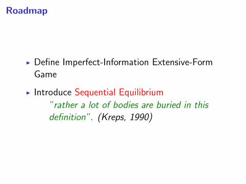
I Define Imperfect-Information Extensive-FormGame

I Introduce Sequential Equilibrium

”rather a lot of bodies are buried in thisdefinition”. (Kreps, 1990)

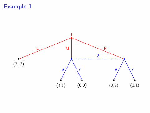
Example 1

1

2

L M R

a r a r(2, 2)

(3,1) (0,0) (0,2) (1,1)

Example 2

L R

RL

0 1

0

1

Def. of Imperfect-Information Extensive-Form GamesI An imperfect-information extensive-form game is a tuple

(N ,H ,P , I, u)I (N,H,P, u) is a perfect-information extensive-form gameI I = {I1, I2, ..., In} is the set of information partitions of

all playersI Ii = {Ii,1, ...Ii,ki } is the information partition of player iI Ii,j is an information set of player iI Action set A(h) = A(h′) if h and h′ are in Ii,j , denote as

A(Ii,j)I P(Ii,j) be the player who plays at information set Ii,j .

I1 = {{Φ}, {(L,A), (L,B)}}, I2 = {{L}}

L R

a b a b

A B

(0,0) (1,2) (1,2) (0,0)

(2,1)

1

1

2

Pure Strategies: Example 3

I S = {S1, S2}I S1 = {(L, a), (L, b), (R , a), (R , b)}I S2 = {A,B}

L R

a b a b

A B

(0,0) (1,2) (1,2) (0,0)

(2,1)

1

1

2

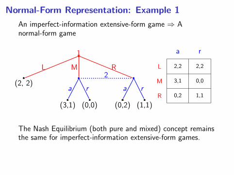
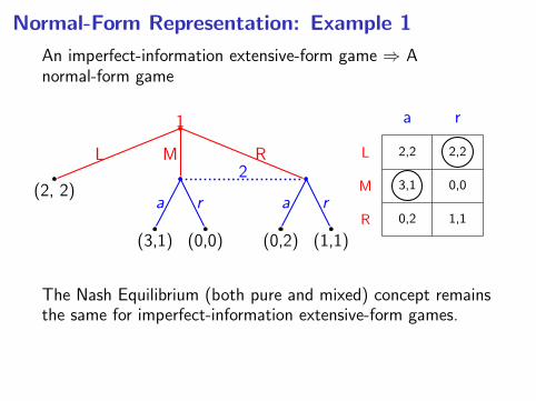
Normal-Form Representation: Example 1

An imperfect-information extensive-form game ⇒ Anormal-form game

1

2L M R

a r a r(2, 2)

(3,1) (0,0) (0,2) (1,1)

L

M

R

a r

2,2 2,2

3,1 0,0

0,2 1,1

The Nash Equilibrium (both pure and mixed) concept remainsthe same for imperfect-information extensive-form games.

Normal-Form Representation: Example 1

An imperfect-information extensive-form game ⇒ Anormal-form game

1

2L M R

a r a r(2, 2)

(3,1) (0,0) (0,2) (1,1)

L

M

R

a r

2,2 2,2

3,1 0,0

0,2 1,1

The Nash Equilibrium (both pure and mixed) concept remainsthe same for imperfect-information extensive-form games.

Normal-Form Games

A normal-form game ⇒ An imperfect-informationextensive-form game

5, 5 0, 8

8, 0 1, 1

C

D

C D

Prisoner’s Dilemma

C D

C D DC

(5,5) (0,8) (8,0) (1,1)

1

2

Nash Equilibrium: Example 1

1

2L M R

a r a r(2, 2)

(3,1) (0,0) (0,2) (1,1)

L

M

R

a r

2,2 2,2

3,1 0,0

0,2 1,1

Suppose we want to generalize the idea of subgame perfectequilibrium. Consider the equilibrium (L, r). Is it subgameperfect?

Nash Equilibrium: Example 1

1

2L M R

a r a r(2, 2)

(3,1) (0,2) (0,2) (1,1)

L

M

R

a r

2,2 2,2

3,1 0,2

0,2 1,1

Suppose we want to generalize the idea of subgame perfectequilibrium. Consider the equilibrium (L, r). Is it subgameperfect?

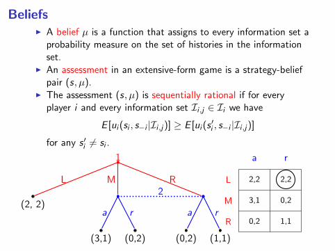
BeliefsI A belief µ is a function that assigns to every information set a

probability measure on the set of histories in the informationset.

I An assessment in an extensive-form game is a strategy-beliefpair (s, µ).

I The assessment (s, µ) is sequentially rational if for everyplayer i and every information set Ii ,j ∈ Ii we have

E [ui (si , s−i |Ii ,j )] ≥ E [ui (s′i , s−i |Ii ,j )]

for any s ′i 6= si .

1

2L M R

a r a r(2, 2)

(3,1) (0,2) (0,2) (1,1)

L

M

R

a r

2,2 2,2

3,1 0,2

0,2 1,1

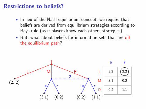
Restrictions to beliefs?

I In lieu of the Nash equilibrium concept, we require thatbeliefs are derived from equilibrium strategies according toBays rule (as if players know each others strategies).

I But, what about beliefs for information sets that are offthe equilibrium path?

1

2L M R

a r a r(2, 2)

(3,1) (0,2) (0,2) (1,1)

L

M

R

a r

2,2 2,2

3,1 0,2

0,2 1,1

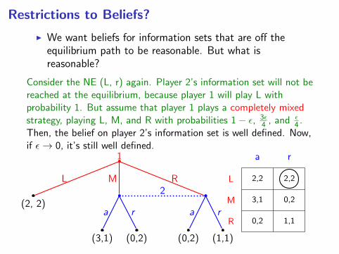
Restrictions to Beliefs?

I We want beliefs for information sets that are off theequilibrium path to be reasonable. But what isreasonable?

Consider the NE (L, r) again. Player 2’s information set will not bereached at the equilibrium, because player 1 will play L withprobability 1. But assume that player 1 plays a completely mixedstrategy, playing L, M, and R with probabilities 1− ε, 3ε

4 , and ε4 .

Then, the belief on player 2’s information set is well defined. Now,if ε→ 0, it’s still well defined.

1

2L M R

a r a r(2, 2)

(3,1) (0,2) (0,2) (1,1)

L

M

R

a r

2,2 2,2

3,1 0,2

0,2 1,1

Consistent Assessment

I An assessment (s, µ) is consistent if there is a sequence((sn, µn))∞n=1 of assessments that converges to (s, µ) andhas the properties that each strategy profile sn iscompletely mixed and that each belief system µn isderived from sn using Bayes rule.

Sequential Equilibrium

I An assessment (s, µ) is a sequential equilibrium of a finiteextensive-form game with perfect recall if it is sequentiallyrational and consistent.

I Thm: Every finite extensive-form game with perfect recallhas a sequential equilibrium.

I A sequential equilibrium is a Nash equilibrium.

I With perfect information, a subgame perfect equilibriumis a sequential equilibrium.

Bayesian Games

Yiling Chen

September 12, 2012

So far

Up to this point, we have assumed that players know allrelevant information about each other. Such games are known

as games with complete information.

Games with Incomplete Information

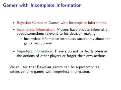
I Bayesian Games = Games with Incomplete Information

I Incomplete Information: Players have private informationabout something relevant to his decision making.

I Incomplete information introduces uncertainty about thegame being played.

I Imperfect Information: Players do not perfectly observethe actions of other players or forget their own actions.

We will see that Bayesian games can be represented asextensive-form games with imperfect information.

Example 4: A Modified Prisoner’s Dilemma Game

With probability λ, player 2 has the normal preferences asbefore (type I), while with probability (1− λ), player 2 hatesto rat on his accomplice and pays a psychic penalty equal to 6years in prison for confessing (type II).

λ

5, 5 0, 8

8, 0 1, 1

C

D

C D

Type I

1− λ

5, 5 0, 2

8, 0 1, -5

C

D

C D

Type II

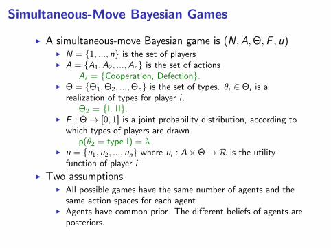
Simultaneous-Move Bayesian Games

I A simultaneous-move Bayesian game is (N ,A,Θ,F , u)I N = {1, ..., n} is the set of playersI A = {A1,A2, ...,An} is the set of actions

Ai = {Cooperation, Defection}.I Θ = {Θ1,Θ2, ...,Θn} is the set of types. θi ∈ Θi is a

realization of types for player i .Θ2 = {I, II}.

I F : Θ→ [0, 1] is a joint probability distribution, according towhich types of players are drawn

p(θ2 = type I) = λI u = {u1, u2, ..., un} where ui : A×Θ→ R is the utility

function of player i

I Two assumptionsI All possible games have the same number of agents and the

same action spaces for each agentI Agents have common prior. The different beliefs of agents are

posteriors.

Imperfect-Information Extensive-FormRepresentation of Bayesian Games

I Add a player Nature who has a unique strategy ofrandomizing in a commonly known way.

Nature

λ 1− λ

C D DC

C D C D DCDC

1

2 2

(5, 5) (0, 8) (8,0) (1, 1) (5, 5) (0, 2) (8, 0) (1, -5)

Strategies in Bayesian Games

I A pure strategy si : Θi → Ai of player i is a mapping fromevery type player i could have to the action he would playif he had that type. Denote the set of pure strategies ofplayer i as Si .S1 = {{C}, {D}}S2 = {{C if type I, C if type II}, {C if type I, D if typeII}, {D if type I, C if type II}, {D if type I, D if type II}}

I A mixed strategy σi : Si → [0, 1] of player i is adistribution over his pure strategies.

Best Response and Bayesian Nash Equilibrium

We use pure strategies to illustrate the concepts. But theyhold the same for mixed strategies.

I Player i ’s ex ante expected utility is

Eθ[ui (s(θ), θ)] =∑θi∈Θi

p(θi )Eθ−i[ui (s(θ), θ)|θi ]

I Player i ’s best responses to s−i (θ−i ) is

BRi = arg maxsi (θi )∈Si

Eθ[ui (si (θi ), s−i (θ−i ), θ)]

=∑θi∈Θi

p(θi )

(arg max

si (θi )∈Si

Eθ−i[ui (si (θi ), s−i (θ−i ), θ)|θi ]

)I A strategy profile si (θi ) is a Bayesian Nash Equilibrium iif∀i si (θi ) ∈ BRi .

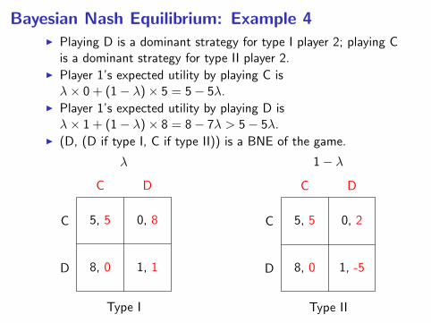
Bayesian Nash Equilibrium: Example 4I Playing D is a dominant strategy for type I player 2; playing C

is a dominant strategy for type II player 2.I Player 1’s expected utility by playing C isλ× 0 + (1− λ)× 5 = 5− 5λ.

I Player 1’s expected utility by playing D isλ× 1 + (1− λ)× 8 = 8− 7λ > 5− 5λ.

I (D, (D if type I, C if type II)) is a BNE of the game.

λ

5, 5 0, 8

8, 0 1, 1

C

D

C D

Type I

1− λ

5, 5 0, 2

8, 0 1, -5

C

D

C D

Type II

Example 5: An Exchange Game

I Each of two players receives a ticket t on which there is anumber in [0,1].

I The number on a player’s ticket is the size of a prize thathe may receive.

I The two prizes are identically and independentlydistributed according to a uniform distribution.

I Each player is asked independently and simultaneouslywhether he wants to exchange his prize for the otherplayer’s prize.

I If both players agree then the prizes are exchanged;otherwise each player receives his own prize.

A Bayesian Nash Equilibrium for Example 5

I Strategies of player 1 can be describe as “Exchange ift1 ≤ k”

I Given player 1 plays such a strategy, what is the bestresponse of player 2?

I If t2 ≥ k , no exchangeI If t2 < k , exchange when t2 ≤ k/2

I Since players are symmetric, player 1’s best response is ofthe same form.

I Hence, at a Bayesian Nash equilibrium, both players arewilling to exchange only when ti = 0.

Signaling (Sender-Receiver Games)

I There are two types of workers, bright and dull.

I Before entering the job market a worker can choose to getan education (i.e. go to college), or enjoy life (i.e. go tobeach).

I The employer can observe the educational level of theworker but not his type.

I The employer can hire or reject the worker.

Example 6: Signaling

Nature

λ 1− λBright Dull

C B BC

H R H R RHRH

Worker Worker

EmployerEmployer

(2, 2) (-1, 0) (4,-1) (1, 0) (2, 1) (-1, 0) (4, -2) (1, 0)

Bayesian Extensive Games with Observable Actions

I A Bayesian extensive game with observable actions is(N ,H ,P ,Θ,F , u)

I (N,H,P) is the same as those in an extensive-form game withperfect information

I Θ = {Θ1,Θ2, ...,Θn} is the set of types. θi ∈ Θi is arealization of types for player i .

Θ1 = {Bright, Dull}.I F : Θ→ [0, 1] is a joint probability distribution, according to

which types of players are drawnp(θ1 = Bright) = λ

I u = {u1, u2, ..., un} where ui : Z ×Θ→ R is the utilityfunction of player i . Z ∈ H is the set of terminal histories.

Best Responses for Example 6I E.g. If the employer always plays H, then the best

response for the worker is B.I But how to define best responses for the employer?

I Beliefs on information setsI Beliefs derived from strategies

Nature

λ 1− λBright Dull

C B BC

H R H R RHRH

Worker Worker

EmployerEmployer

(2, 2) (-1, 0) (4,-1) (1, 0) (2, 1) (-1, 0) (4, -2) (1, 0)

A Bayesian Nash Equilibrium of Example 6

Nature

λ 1− λBright Dull

C B BC

H R H R RHRH

Worker Worker

EmployerEmployer

(2, 2) (-1, 0) (4,-1) (1, 0) (2, 1) (-1, 0) (4, -2) (1, 0)

λ 1− λ

p(Bright|Beach) =p(Bright)σ(Beach|Bright)

p(Bright)σ(Beach|Bright)+p(Dull)σ(Beach|Dull)= λ·1

λ·1+(1−λ)·1 = λ

“Subgame Perfection”

I The previous Bayesian Nash Equilibrium is not “subgameperfect”. When the information set College is reached,the employer should choose to hire no matter what beliefhe has.

I We need to require sequential rationality even foroff-equilibrium-path information sets.

I Then, beliefs on off-equilibrium-path information setsmatter.

Perfect Bayesian Equilibrium

A strategy-belief pair, (σ, µ) is a perfect Bayesian equilibriumif

I (Beliefs) At every information set of player i , the playerhas beliefs about the node that he is located given thatthe information set is reached.

I (Sequential Rationality) At any information set of player i ,the restriction of (σ, µ) to the continuation game must bea Bayesian Nash equilibrium.

I (On-the-path beliefs) The beliefs for anyon-the-equilibrium-path information set must be derivedfrom the strategy profile using Bayes’ Rule.

I (Off-the-path beliefs) The beliefs at anyoff-the-equilibrium-path information set must bedetermined from the strategy profile according to BayesRule whenever possible.

Perfect Bayesian Equilibrium

I Perfect Bayesian equilibrium is a similar concept tosequential equilibrium, both trying to achieve some sort of“subgame perfection”.

I Perfect Bayesian equilibrium is defined for allextensive-form games with imperfect information, not justfor Bayesian extensive games with observable actions.

I Thm: For Bayesian extensive games with observableactions, every sequential equilibrium is a Perfect Bayesianequilibrium.

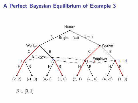
A Perfect Bayesian Equilibrium of Example 3

Nature

λ 1− λBright Dull

C B BC

H R H R RHRH

Worker Worker

EmployerEmployer

(2, 2) (-1, 0) (4,-1) (1, 0) (2, 1) (-1, 0) (4, -2) (1, 0)

β 1− βλ 1− λ

β ∈ [0, 1]

Summary of Equilibrium Concepts

On-equ-pathstrategy σon

On-equ-pathbelief µon

Off-equ-pathstrategy σoff

Off-equ-pathbelief µoff

NE BR N/A N/A N/A

BNE BR given µon Consistentwith σon

N/A N/A

SPNE BR N/A BR N/A

PBE BR given µon Consistentwith σon

BR given µoff Consistentwith σoff

SE BR given µon Consistentwith σon

BR given µoff Consistentwith σoff