learning in extensive-form games: experimental data...

GAMES AND ECONOMIC BEHAVIOR 8, 164--212 (1995)

Learning in Extensive-Form Games: Experimental Data and Simple Dynamic Models in the

Intermediate Term*

ALVIN E . ROTH AND IDO EREV

Tile University of Pittsburgh, Pittsburgh, Pennsylvania, 15260; and The Technion, 32 000 Haifa, Israel

Received July 30, 1993

We use simple learning models to track the behavior observed in experiments concerning three extensive form games with similar perfect equilibria. In only two of the games does observed behavior approach the perfect equilibrium as players gain experience. We examine a family of learning models which possess some of the robust properties of learning noted in the psychology literature. The intermediate term predictions of these models track well the observed behavior in all three games, even though the models considered differ in their very long term predictions. We argue that for predicting observed behavior the intermediate term predictions of dynamic learning models may be even more important than their asymptotic properties. Journal of Economic Literature Classification Num- bers: C7, C92. © 1995 Academic Press. Inc.

I. INTRODUCTION

No one can look widely at experimental data without noticing that experience matters. At least for the first few times a game is played, observed behavior is likely to change as players acquire experience, in a way that suggests that learning is important--learning not only about the structure of the game being played, but also about the behavior of the

* Prepared for the Nobel Symposium on Game Theory, June 18-20, 1993, Bj6rkborn, Sweden. This work was supported in part by NSF Grant SES-9121968, and much of the work was completed while Erev was a Visiting Postdoctoral Fellow in Economics at the University of Pittsburgh. We thank Antonio Cabrales, David Cooper, Vince Crawford, John Duffy, Drew Fudenberg, John Kagel, Jack Ochs, Emilie Roth, Xiaolin Xing, and Shmuel Zamir for helpful comments.

164 0899-8256/95 $6.00 Copyright © 1995 by Academic Press, Inc. All rights of reproduction in any form reserved.

LEARNING IN GAMES: DATA AND MODELS 165

other players. (This is an observation that can be made with field data also, a point to which we will return in the conclusion.) So it is natural to consider how well we can explain observed behavior in terms of adaptation. And, while adaptative behavior may potentially be quite complex, it is useful to see how much of what we observe can be explained with very simple models of adaptation.

This paper considers the behavior observed in experiments with three different two-stage sequential games; a public goods provision game, a market game, and an "ultimatum" bargaining game, which will all be described shortly. The three games have in common not only a two-stage, alternating move structure, but also that the perfect equilibrium prediction for each game is that all or almost all of the gains will be captured by one player. However, the observed behavior for the three games is different. For the public goods and market games, under a variety of conditions involving different subject pools and different information about payoffs, behavior is observed to converge quickly to the perfect equilibrium prediction. But in the ultimatum game, also under a variety of conditions, behavior is observed to be far from the perfect equilibrium prediction even after players have gained a reasonable amount of experience. Furthermore, the behavior observed in the ultimatum game is different in different subject pools, and appears to become more different as the players acquire experience.

We consider adaptive models from a simple family of dynamics, in which players increase the probability of playing pure strategies that have met with success in previous periods. These simple dynamics do a surpris- ingly good job of reproducing the major features of the experimental data. Each dynamic we consider from this family converges quickly to the perfect equilibrium of the public goods and market games, from a wide range of initial conditions. However these same dynamics do not converge quickly, if at all, to the perfect equilibrium of the ultimatum game, and their behavior in the ultimatum game is sensitive to the initial conditions. In fact, when we initiate each of the dynamics with initial conditions estimated from those observed experimentally in different subject pools, we see the dynamic paths diverge in much the same way as the ultimatum game data.

One lesson we will seek to draw, therefore, concerns differences among the games, captured by the fact that the same dynamic models make different predictions for the different games. Both the experimental and computational results we report support the intuition that we can expect to find classes of games in which certain kinds of equilibrium are quickly observed, and others in which they are not. And some games are relatively insensitive to initial conditions, while in other games initial conditions are important.

166 ROTH AND EREV

A second lesson concerns which aspects of dynamic models offer testable predictions. While almost all of the theoretical literature on adaptive dynamics has focused on the very long term, via theorems about convergence as time goes to infinity, we will argue that intermediate term results (such as paths, velocities, and transit durations) may be even more important. To make this argument, we will consider particular dynamic models with quite different long term propertiesmmodels whose asymptotic predictions approach perfect equilibria, imperfect equilibria, and non-equilib- r i a - a n d observe that these models nevertheless make similar intermediate term predictions for these three games. We will argue that, both because it would be difficult to distinguish among these different dynamics on the basis of data, and because dynamic models are more likely to be informative when the learning curve is steep than when it is flat, there is reason to pay attention to their intermediate term predictions. (Although we will not try to precisely define what constitutes the "intermediate" term, our operational definition will be to take the intermediate term predictions of a model to be those it makes as the learning curve begins to be very flat.)

To use an analogy, even if we believe that time and the tide eventually turn all coastlines into sandy beaches, knowing the difference between granite and sandstone is a great help in understanding why, in the intermediate term, some coastlines have rocky cliffs.

To summarize, this paper makes several kinds of comparisons. We demonstrate differences among the games by looking at a single dynamic model (at a time) and observing that it acts differently on the different games. And we demonstrate which aspects of the dynamic models seem to us to be potentially most descriptive of observed behavior, and most testable, by looking at the predictions of several dynamic models simultaneously, and comparing them to each other and to the experimental data. We will see that the intermediate term predictions of all the models we consider are similar both to each other and to the experimental data, even though the long term predictions of these models can be quite different (both from each other and from the experimental data).

This paper will be organized as follows. Section II presents the experimental games and observed outcomes. Section III introduces the family of dynamic models we consider. Section IV presents the details of the computational models of the games--i t explains how and why we represent the strategy spaces in the three games by smaller sets than were actually available in the experiments. Section V studies the differences among the three games by comparing the dynamics they induce when the initial conditions are randomly generated. Section VI presents the predictions of these dynamic models about the experimental games, starting from the observed initial conditions, and compares them with each


other and with the experimental data. Section VII concludes with a sum- mary of what we think we have learned, some directions for further work, and some final reflections on intermediate term versus long term predictions.

I I . EXPERIMENTAL DATA

The data we consider come from two papers: Roth et al. (1991); and Prasnikar and Roth (1992). The first of those papers compares the behavior observed in a two-player ultimatum bargaining game and a ten-player market game (of the "one right shoe, nine left shoes" variety) played under comparable conditions in four countries.~ The games and the environment in which they were played are described as follows (Roth et al. (1991) pp. 1068-1169):

The two-player bargaining environment we look at is an ultimatum game: one bargainer makes a proposal of how to divide a certain sum of money with another bargainer, who has the opportunity to accept or reject the proposed division. If the second bargainer accepts, each bargainer earns the amount proposed for him by the first bargainer, and if the second bargainer rejects, then each bargainer earns zero. To allow us to observe the effects of experience, subjects in the bargaining part of the experiment each participate in ten bargaining sessions against different opponents. Although different pairs of bargainers interact simultaneously, each bargainer learns only the result of his own negoti- ation.

The multi-player market environment we examine has a similar structure: multiple buyers (nine, in most sessions) each submit an offer to a single seller to buy an indivisible object worth the same amount to each buyer (and nothing to the seller). The seller has the opportunity to accept or reject the highest price offered. If the seller accepts then the seller earns the highest price offered, the buyer who made the highest offer (or, in case of ties, a buyer selected by lottery from among those who made the highest offer) receives the difference between the object's value and the price he offered, and all other buyers receive zero. If the seller rejects, then all players receive zero. Each player learns whether a transaction took place, and at what price. To allow us to observe the effects of experience, subjects in the market part of the experiment each participate in ten markets, with a changing population of buyers.

i These were Israel, Japan, Slovenia (when it was still part of Yugoslavia), and the U.S.A. Ultimatum game experiments have been reported by Guth et al. (1982), and by many others since, along with sequential bargaining games having more periods (inspired in part by the theoretical work of Stahl, 1972, and Rubinstein, 1982, on multiperiod games). Both in the one-period ultimatum games and in the longer bargaining games, experimental results typically diverge from the perfect equilibrium predictions (see, e.g., Ochs and Roth, 1989, or Bolton, 1991, or see Roth, 1994, for a survey of such bargaining experiments). "Right shoe left shoe" games have been a source of theoretical examples for a long time; some earlier experimental results are reported in Murnighan and Roth (1980).

168 ROTH AND EREV

In both the market and bargaining environment, the prediction of the unique subgame perfect equilibrium (under the auxiliary assumption that subjects seek to maximize their monetary payoffs) is that one player will receive all the wealth (or almost all, if payoffs are discrete).

We note in passing that many interesting problems of experimental design arise in conducting an experiment in four countries, if one wishes to control for the fact that the data are collected by different experimenters, and subjects are instructed in different languages and paid in different currencies. We refer the reader to Roth et al. (1991) for how these problems were addressed. 2 For our present purposes, it is enough to note that the experiment gives us data about each game from subjects who played the game 10 times, but against different opponents each time (in order that the one-shot character of each game be preserved). Thus subjects gained experience with the game at the same time as they encountered other subjects who had gained a similar amount of experience. (Subjects played the same role in all rounds--e.g. , a subject who was a player I in the ultimatum game would be a player 1 in all 10 rounds.)

All transactions were carried out in terms of "1000 tokens" with a smallest divisible unit of 5 tokens. Note the similarity in the equilibrium structure of the two games. At the perfect equilibria of both the ultimatum and market games, one player's payoff is either 995 or 1000; in the market game the perfect equilibrium offers are 995 or 1000, and in the ultimatum game these are the perfect equilibrium demands (for himself) by the pro- poser. But for both games any offer can be made at a nonperfect Nash equilibrium. Nevertheless, the behavior observed in the two games is different; quickly approaching perfect equilibrium in the market game in all four countries, and remaining far from perfect equilibrium in the ultimatum game. 3

In the market game, offers made in round 1 were dispersed, but equilibrium was reached in all four countries by round I0, with from almost 40% to over 70% of all offers being at the highest feasible prices in the different subject pools. (Note that perfect equilibrium is achieved in a given market whenever two or more offers of 1000 are made, so that no prediction is made about the dispersal of lower offers.)

2 We emphasize that the details of how experiments are conducted are often of critical importance in understanding the results. We skip over many details so lightly here not merely because they are published elsewhere, but because they are important primarily for evaluating the differences observed between subject pools. We are content to leave unexplained here those differences observed in the first periods of play, and we will show that the remaining differences can largely be explained via the adaptive models we consider.

3 To conserve space, we must content ourselves below with a verbal description of the data, which are described much more completely, of course, in the original papers. Later in the paper we will offer more formal comparisons of the learning simulations and the data from these experiments (see, e.g., the first (data) columns of Figs. 4-6).


The ultimatum game data tell a very different story. In round 1, the same modal demand, of 500, was observed in each country. But in round 10, the modal demands were still 500 in the U.S. and Slovenia, while in Japan there were modes at 550 and 600, and in Israel there was a mode at 600. These differences in the modes reflect significant differences in the distributions of observed demands. 4 That is, unlike what we saw in the market game, tenth round demands in the ultimatum game did not begin to approach the perfect equilibrium, and there were significant differences among the subject pools.

The paper by Prasnikar and Roth compared ultimatum and market games with a third game called a "best shot" game. The best shot game is a two-player game whose rules are that player 1 states a quantity ql, after which player 2, informed of q j , states a quantity q2- An amount of public good equal to the m a x i m u m of qj and q2 (the "best shot") results, and each player i receives a payoff which is a function of that quantity of public good (q = max{ql, q2}) minus $0.82 times qi (see Table I). The perfect equilibrium prediction is that player 1 will choose q~ = 0 and player 2 will choose q2 = 4, giving player 1 a profit of $3.70 and player 2 a $0.42 profit. 5 Prasnikar and Roth (1992) observed these games under two information conditions. Subjects in the full information condition knew that both players had the same payoff table (Table I), while subjects in the partial information condition knew only that Table I determined their own payoffs-- they did not know how the other player's payoffs were determined. As in the ultimatum and market games, each subject participated in ten one-shot games against different opponents, always in the same position (player 1 or player 2). 6 In both information conditions the players learned quickly not to both provide positive quantities. In the full information condition (but not the partial information condition) every

4 The observed distributions are significantly different for every pair of countries except the U.S.A. and Slovenia, and the between country differences are larger than the differences between groups within a given country. (Because the distributions are highly asymmetric, the statistical test used is the Mann-Whitney U test, which is based on the rank of each observation in the sample distribution.)

5 Thus the ratio of predicted payoffs to the two players is nine to one. To see that (ql = 0, q2 = 4) is the unique perfect equilibrium outcome, observe from Table I that if player l provides ql = 0, then player 2's unique best response is to provide q2 = 4 , since the first four units of public good all have a higher marginal value than the cost to player 2 of providing each unit, while the fifth unit of public good has a lower marginal value. And if player 1 provides a quantity ql -> l, then player 2's unique best response is to provide q2 = 0 , which gives player l a strictly lower payoff than if he provides 0 and player 2 provides 4. Note there is one other outcome, ql = 4, q2 = 0 , which can occur at a Nash equilibrium (but not at a perfect equilibrium).

6 Harrison and Hirshleifer (1989) had earlier reported experimental results for the best shot game under the partial information condition, similar to those discussed here.

170 ROTH AND EREV

TABLE I

REDEMPTION VALUES AND EXPENDITURE VALUES FOR THE BEST SHOT FULL AND PARTIAL INFORMATION GAMES

Redemption values Expenditure values

Redemption Number of Cost to you of the Project level value of Total redemption units you number units you (units of q) specific units value of all units provide provide

0 $0.00 $0.00 0 $0.00 1 1,00 1.00 I 0.82 2 0,95 1.95 2 1.64 3 0.90 2.85 3 2.46 4 0.85 3.70 4 3.28 5 0.80 4.50 5 4.10 6 0,75 5.25 6 4.92 7 0,70 5.95 7 5.74 8 0,65 6.60 8 6.56 9 0.60 7.20 9 7.38

10 0,55 7.75 10 8.20 11 0,50 8.25 I 1 9.02 12 0,45 8.70 12 9.84 13 0.40 9.10 13 10.66 14 0.35 9.45 14 11.48 15 0.30 9.75 15 12.30 16 0.25 10.00 16 13.12 17 0.20 10.25 17 13.94 18 0.15 10.35 18 14.76 19 0.10 10.45 19 15.58 20 0.05 10.50 20 16.40 21 0.00 10.50 21 21.22

player 1 learned (before round 10) to provide q l = 0. And in both conditions the perfect equilibrium outcome (q~, q2) = (0, 4) was the modal outcome by round 10, although convergence towards the perfect equilibrium was faster in the full information condition than in the partial information condition.

Thus all of these three games have extreme perfect equilibrium predictions, and the experimental results (nevertheless) show quick convergence to the perfect equilibrium in the market game and best shot game in the full information condition, somewhat slower convergence in the best shot game with partial information, and no apparent approach to perfect equilibrium at all in the ultimatum game. We turn next to see what insight into this behavior we can derive from a family of very simple learning models.


I I I . A FAMILY OF ADAPTIVE MODELS

We describe here a family of stochastic dynamic models of individual behavior, which determine the probability that a given player will choose a given pure strategy at time t, and how these probabilities evolve over time in response to the player's experience. We defer to Sections V and VI the descriptions of the multiplayer interactions in the computational simulations.

Our selection of dynamic models has been guided by three principle criteria. First, the models should be consistent with the robust properties of learning observed in the large experimental psychology literature on both human and animal learning. Perhaps the most robust of these properties is that choices that have led to good outcomes in the past are more likely to be repeated in the future. (This result, known as the "Law of Effect," has been observed in a very wide variety of environments at least since Thorndike, 1898.) Another robust observation is that learning curves tend to be steep initially, and then flatter. (This observation is known as the "Power Law of Practice," and dates back at least to Black- burn, 1936. 7 )

The second criterion is that the model of how an individual changes his behavior in response to his experience should not depend on observations that cannot be made by the players in the experimental environments in question. In particularl in each game we consider there are information sets not reached on any given play of the game, so players cannot observe one another's strategies, only their choices. For example in the ultimatum game, if a player observes that a certain offer was rejected, he cannot observe which offers would have been accepted, and vice versa. 8

The third criterion is that the models should not depend on observations about the players that cannot be observed in the experimental data. While the experimental data we consider reveal more than can be observed by

7 A typical expression of this "power law," from which it derives its name, is that the relationship between the time T it takes to perform a task, as a function of how many times P it has been practiced, often fits well a curve of the form T = a P -b for constants a and b, so that the decrease in time corresponding to increased practice quickly becomes small.

s This rules out dynamic models such as "fictitious play," in which players observe each other 's full pure strategies. Robinson (1951) showed that fictitious play converges to the Nash equilibrium for two-player zero sum games, and Shapley (1964) showed a non-conver- gent two-person nonzero-sum counterexample. Recently there has been renewed interest in convergence results for this and related dynamic models: see, e.g., Aoyagi (1992), Fuden- berg and Kreps (1993), Krishna (1992), Milgrom and Roberts (1991), and Monderer and Shapley (1992). There has also been some recent theoretical interest in notions of equilibrium which arise when players cannot observe each other 's strategies, but only their behavior at information sets which are reached: see, e.g., Fudenberg and Levine (1993a,b) and Kalai and Lehrer (1993).

172 ROTH AND EREV

any individual player in the experiment (e.g., about distributions of choices across the population of players) the data do not reveal what players initially believe, or how they update their beliefs. We have chosen not to construct models with unobservable parameters for each individual. 9

An additional criterion, harder to make precise, is that the models should be simple. The models we consider here will all be variations on the following basic model, which can be applied to games with finite pure strategy sets.

A. The Basic Mode l

At time t = 1 (before any experience has been acquired) each player n has an initial propensity to play his kth pure strategy, given by some number q,,~(l). If player n plays his kth pure strategy at time t and receives a payoff of x, then the propensity to play strategy k is updated by setting q,x(t + I) = q,,k(t) + x, while for all other pure strategies j , q,,i(t + 1) = q,o(t). The probability p,,~(t) that player n plays his kth pure strategy at time t is p,,k(t) = q,,k(t)/Eq,,j(t), where the sum is over all of player n's pure strategies j.

So pure strategies which have been played and have met with success tend over time to be played with greater frequency than those which have met with less success; i.e. these dynamics obey the "law of effect." Also, the learning curve will be steeper in early periods and flatter later (because Eq,j(t) is an increasing function of t, so a payoff of x from playing pure strategy k at time t has a bigger effect on p,,k(t) when t is small than when t is large; i.e., the derivative of pnk(t) will respect to a payoff of x is a decreasing function of t). This latter property will permit our loose operational definition for the "intermediate t e r m " - - as the steep part of the learning curve gives way to the flat part, the short term ends and the intermediate term begins.

These learning dynamics have a certain resemblance to evolutionary dynamics (cf. Maynard Smith, 1982) even though they are not the "replica- tor" dynamics customarily associated with evolutionary models, l0 (In fact

9 That is not to say of course that such beliefs may not play a role, even an essential role, in players' behavior. There have recently been a number of interesting Bayesian models which explore long term convergence to Nash equilibria (e.g., Jordan, 1991; Kalai and Lehrer, 1993; and N yarko, 1992). Of particular interest is Crawford (1992), which estimates belief parameters for agents from the experimental data of Van Huyck et al. (1990, 1991) and uses these estimates to run simulations of their experiments which agree well with the experimental observations. We discuss in the conclusion how players' knowledge and beliefs might be influencing their behavior in the data we consider, despite the good results we get from models which ignore these factors.

to See e.g. Friedman (1991) for a discussion of a broad class of evolutionary dynamics characterized by the fact that successful strategies increase their share of the population. And see Selten (1991) for a nontechnical discussion of the roles that both inherited and


this model was proposed as an approximation of evolutionary dynamics by Harley, 1981). The chief point of similarity is that the influence of other players' past behavior on any player n's behavior at time t is via the effect that their behavior has had on player n's past payoffs.

This model is also quite similar to that of Bush and Mosteller (1955) (which was employed by Cross, 1983 to explain economic behavior), but it has some significant differences. Bush and Mosteller's model also obeys the law of effect, but, unlike the model we consider, their learning curves need not get flatter over time.~t

The simple model we consider does not require (or permit) a player to observe the full strategies of other players, or to make calculations based on other players' payoffs. So it can be applied to the kinds of games we consider here in which players only observe one another's choices, not their strategies. And it can be applied to the best shot games under both full and partial information.

B. Some Modifications

Here we introduce three modifications of the basic model. The first has a "cutoff" parameter/z which prevents events with unobservably small probabilities from influencing the outcome. The second modification has an "experimentation" (or "error" or "generalization") parameter e which prevents the probability of a strategy from going to zero if it is "c lose" to a successful strategy. The third modification introduces a "forgetting" parameter ~, which speeds convergence by preventing the sum of any player n's propensities, Eq,,j(t), from growing without bound as t goes to infinity. When/x, e, and ~ all equal zero, we have the basic model described above.

noninherited characteristics might play in learning in economic environments. Evolutionary models have been compared with experimental data by Crawford (1991) (for a series of coordination experiments the first of which is reported by Van Huyck et al. (1990)), and by Miller and Andreoni (1991) who considered the stylized facts from a number of public goods experiments. Another, more complex kind of biologically motivated model is that of "genetic algorithms" (Holland, 1975), which involve mating as well as selection. (See also Holland and Miller, 1991, for some further thoughts on using genetic algorithms to model economic behavior.) Arthur (1991, 1993) uses some individual choice data reported by Bush and Mosteller (1955) to calibrate a model very closely related to the basic model considered here (except that the rate of learning is kept constant by renormalizing the sum of the propensities after each choice), and reports a good fit with the learning behavior reported in that experiment.

11 Bush and Mosteller's model updates the probabilities of choosing each strategy directly, without the intermediate "propensities" we employ. This has the effect (which Bush and Mosteller, 1955 p. 17, refer to as "Independence-of-path") of making the magnitude of change in any period dependent only on the current probabilities and not on the amount of previous experience. Their model also differs from the one we consider here in that it cannot converge to a pure strategy in an uncertain environment in which the post-hoc best response (but not the expected best response) changes from trial to trial.

174 ROTH AND EREV

1. Ext inct ion in Fini te Time

The first modification allows the probabilities pnk(t) t o go to zero in finite time. We do this by simply truncating to zero probabilities which fall below some small "cutoff" probability/z. That is, whenever in the basic model we get phi(t) = q,,k(t)/Y,q,,j(t) < /~, we set p,,k(t) = q,,k(t) = 0 instead. This has several advantages and some (potential) disadvantages. Not least of the advantages is that it allows us to avoid predicting that the long term behavior of the game depends on (intermediate term) events of such low probability that they would have virtually no chance of being observed in the data. It is good to avoid basing predictions on unobservables, when you can. (This also has the practical advantage of preventing roundofferror from becoming a factor in the computational results.) A second advantage is that setting these small probabilities to zero speeds convergence, which can now take place in finite time. Since our argument about the relative merits of intermediate term as opposed to long term results will apply even to the speeded up model, this increases the force of the argument.

Among the potential disadvantages of allowing finite extinction in this way is that it may add unwanted variance--there is even a positive probability that a strictly inferior strategy will persist while superior strategies become extinct. Suppose for example that a player happens to play a strictly dominated strategy that nevertheless yields a small positive payoff. Since this payoff increases his propensity to play this strategy, there is a chance that he will play it again, and again, and a sufficiently long sequence of plays in which he employs only this strategy could result in its probability coming sufficiently close to one so that all other strategies would become extinct. This cannot happen in the next modification of the basic model, which introduces persistent local experimentation.

2. Pers is tent Loca l Exper imenta t ion or Error

The modification we consider now will not employ a cutoff probability (i.e., p~ = 0 in this model), but neither will it allow the probability of playing a strategy to become arbitrarily close to zero if that strategy is "c lose" to a high probability strategy. In particular, we introduce a parameter e which, when it is positive, can be interpreted as guaranteeing persistent local experimentation or error. ~z We do this by changing the way each player updates the propensities to play each pure strategy. If player

n A much more nuanced model of persistent experimentation in extensive form games is given by Fudenberg and Kreps (1988). Kandori et al. (1993) explore an evolutionary model in which persistent experimentation (or mutation, or entry) produces a stationary Markov process with a positive probability of transiting in one step from any state to any other. For related work see Foster and Young (1990), Young 0993), and Binmore and Samuelson (1993).


n plays his kth pure strategy at time t and receives a payoff of x, then the propensity to play strategy k is updated by setting q,k(t + 1) = q,k(t) + ( 1 - e)x. The remaining quantity ex will be added to the propensities to play the strategies adjacent to strategy k, where "adjacent" remains to be precisely defined in Section IV when we describe the simplified games on which the computations are performed. For all other pure strategies j (i.e., for j neither equal to nor adjacent to k), q,j(t + 1) = q,j(t). When e = 0 this model is the same as the basic model. When e is positive, there is persistent "local" experimentation--strategies close to a high probability strategy must also be played with a positive probability that is bounded away from zero.~3

3. Gradual Forgetting

The final modification we consider has a "forgetting" parameter ~o, which limits how flat the learning curve can become. At the end of each period t, each propensity q,o(t) obtained as before is multiplied by I - ~o, e.g. if ~o = 0.001 then each propensity is multiplied by 0.999 to obtain the propensities for the next period. (This has no effect on the p,,~, since the ratios of propensities are unchanged, but it keeps the sum of the propensities from growing without bound.) When Zq,,j(t) is small, this has little effect on player n's rate of learning. But suppose, for example, that player n earns an average payoff of p per round, and that ~o = .001. Then Y~q,o(t) will tend to grow over time until it reaches 1000p, after which the amount gained per round will just equal the amount "forgotten," so that Zq,o(t) will thereafter remain approximately constant (unless player n's average payoff should change). At that point the "weight of the past" will stop growing, and each new payoff will start to have approximately the same influence on player n's propensities. This will allow us to show more clearly how the models diverge in the very long term. For this purpose, we will use a positive forgetting parameter together with a positive experimentation

13 If persistent global experimentation is desired, the residual propensities ex can be distributed over all pure strategies. The choice of local experimentation is motivated in part by the observation that feedback which reinforces a given choice also reinforces similar choices (a phenomenon referred to as "generalization" in the behavioral psychology litera- t u r e - s e e , e.g., Guttman and Kalish, 1956, for an early study of this phenomenon in pigeons). Note that when the states of the system are modeled as being the vector of propensities to play each pure strategy, the resulting stochastic process is a Markov process with an infinite state space, with nonrecurring states (because every agreement increases the sum of the propensities). Thus descriptive simplicity does not insure analytical simplicity. (More generally, the initial steps of a project designed to produce models of observed behavior can be expected to be different from the initial steps of projects directed at showing how equilibria might arise. The two agendas may eventually show signs of convergence . . . . )

176 ROTH AND EREV

parameter, so that we will be considering a model of local experimentation with gradual forgetting.

The local experimentation models (with or without forgetting) have quite different long term properties than the cutoff model. This is easiest to see by noting that the local experimentation models cannot converge to pure strategies (since if strategy k were to be played with probability approaching I - e, the probabilities of strategies k - 1 and k + 1 would eventually each approach e/2). Nevertheless, we will see that the intermediate term predictions of all three models are quite similar. The differences in the models' long term predictions only become apparent in the ultimatum game, and only in the very long term.

4. Parameters of the Models

Within each of the computations which follow, players on the same side of a game will have the same initial propensities, i.e., for each pure strategy k, and for any two players n and m on the same side of the game q,,k(1) = qmk(1). (Of course this equality will not in general hold for times t > 1, since at time t = 1 even players with the same initial propensities will choose different strategies, encounter different behavior from their opponents, etc.) So there are two kinds of choices of initial propensities which will influence the predictions of the model for subsequent times t. The first of these are the ratios q,k(l)/qnj(1) of propensities to play different pure strategies k and j , which determine the relative probabilities that k and j will be played at time t = 1. The second is the sum over all pure strategies j of the initial propensities, which we call the strength of the initial propensities, S(1) = 2q,i(1).

When the initial propensities are strong, i.e. when S(1) is high, learning will be slower than when S(I) is low. (If player n plays pure strategy k at time t = 1 and earns x, the updated probability that he will play k at t = 2 is p,k(2) = (q,,~(1) + (1 - e)x)/(S(1) + x).) In the computations which follow, we will report results for initial strengths of 10, the same order of magnitude as the payoffs in the games.~4

t4 We have briefly examined the models studied here with S(1) = 100 also, which produces somewhat slower initial learning but does not appear to be different in any other way from the parameters we report. Note that the cutoff and experimentation parameters can also influence the importance of each player 's initial experience at time t = 1. When S(l) is small, p. is large, and e = cp = 0, the experience at t = l has the most chance of influencing the long term predictions of the dynamic model, since learning is fast and there is a chance for one strategy to drive out all others. Note also that a model which had both e and/~ positive could behave differently than the local experimentation models we concentrate on, and could have one pure strategy played with probability one in the long term (when the probability of playing an adjacent strategy might fall below the cutoff even after the addition of (e/2)x).


We will report results for the cutoff model with /~ = 0.01 (and e = ~o = 0), for the local experimentation model with e -- 0.05 and O. 1 (and /z = ~o = 0), and for the experimentation model with forgetting with e = 0.05 and O.1, ~o = .001, and/z = O.

IV. THE SIMPLIFIED GAMES USED FOR COMPUTATIONS

The games played in the experiments described earlier have finite pure strategy sets, and so, when we prepare to run a learning model through a simulation of the experiments, we could in principle estimate from the data the initial propensities to play each strategy. The problem with this approach is that it would require enormous amounts of data to estimate reliable probabilities for playing each of so many distinct strategies. Instead, we simplify the games by aggregating the many strategies into a relatively small set of strategies, so that when the data are similarly aggregated, we have a chance of having multiple observations for each strategy of the simplified game. ~5 The games are simplified as follows.

The Simplified Ultimatum Game. Players 1 and 2 each have nine pure strategies. Player 1 chooses a demand d~, which is an integer between 1 and 9, and is the amount player 1 demands for himself. Player 2 chooses a maximal acceptable demand m2, which is also an integer between 1 and 9. If player l ' s demand is acceptable to player 2, i.e., ifd~ -< m2 then player 1 earns d~ and player 2 earns 10 - d~. If the demand is not acceptable, i.e. if d~ > m2 then each player earns 0. So dl and m2 constitute a Nash equilibrium if and only if d~ = m2, while the unique perfect equilibrium is d I = m2 = 9.

The Simplified Best Shot Game. Player I chooses one of three possible contributions q~ = 0, 2 or 4. Player 2 chooses one of 27 response rules:

000, 002, 004, 020, 022, 024, 040, 042, 044, 200, 202, 204, 220, 222, 224, 240, 242, 244, 400, 402, 404,420, 422, 424, 440, 442, 444,

where the first number in each response rule is the amount q2 that player 2 will provide in response to a contribution ofq~ = 0, the second a response to qj = 2 and the third a response to q~ = 4. The payoffs are determined, as in the experiment, from Table I (e.g., at the perfect equilibrium, when

15 Note that even though these are all games of perfect recall, strategies and behavioral strategies are not equivalent for the adaptive models we are considering. We are modeling strategies, not behavioral strategies.

178 ROTH AND EREV

player 1 chooses q~ = 0 and player 2 chooses the response rule 400, the payoffs are (3.70, 0.42), corresponding to the quantities q~ = 0 and q2 = 4).

The Simplified Market Game. Each buyer n chooses one of 11 prices from the set {.25, 1, 2, 3, 4, 5, 6, 7, 8, 9, 9.75}. If the price Pn chosen by buyer n is strictly higher than the price chosen by any other buyer, then buyer n earns 10 - p,, and all the other buyers earn 0. If the maximum price p, is chosen by k buyers, then each one of them earns (I0 - p,)/k, while all the other buyers earn 0. (In this simplified market game we have suppressed the role of the seller, who in the data of Roth et al. (1991) never rejected an offer. It will be apparent that we could have included the seller, modeled like player 2 in the ultimatum game, without substantively changing the results.)

We can now complete our description of how, when the experimentation parameter e is positive, the propensities to play pure strategies are updated for strategies "ad jacen t" to the one most recently played. For the simplified ultimatum and market games, adjacent strategies are determined by the usual order of the real line. For example in the ultimatum game if e = 0.05, and players I and 2 choose d t = 7 and m2 = 8, then player 1 earns 7, and his propensity to choose 7 in the next period is increased by 0.95 × 7 = 6.65 while his propensities to choose 6 and 8 are each increased by 0.175. In the same way, player 2 earns 3 and his propensity to choose 8 is increased by 0.95 × 3 = 2.85, and his propensities to choose 7 and 9 are each increased by 0.075.

If a player has chosen an extreme strategy, such as 9 in the ultimatum game, and earns x, then the propensity to play 8 is increased by (e/2)x as before, while the propensity to play 9 is increased by (1 - e/2)x (instead of by (I - e)x that would have been allocated if there were a higher adjacent strategy). This " ex t r a " (e/2)x allocated to the extreme strategy gives a slight local upward bias to the dynamics of the ultimatum game which we will see is not sufficient to make the ultimatum results approach in the intermediate term the perfect equilibrium prediction that player I will demand 9.16

For the best shot game the situation for player I is exactly analogous to the other two games, but if player 2 plays response rule xyz and player I has chosen q~, the adjacent response rules are those which agree with xyz on those components different from q~. For example if player 1 chooses q l = 2 and player 2 chooses response rule 222, then (from Table I) each

16 If we had chosen instead the option of allocating the extra (el2)x to strategy 8 in this case, it would have produced a slight downward bias, and it might have appeared that this was the cause of the failure to converge to 9.


player receives a payoff of 1.95-1.64 = 0.31, and player 2's propensity to play 222 is increased by (1 - e)(0.31) while his propensities to play 242 and 202 are each increased by (e/2)(0.31).

In Section VI we will report full simulations of the experimental environment, starting from observed initial conditions. First, however, we demonstrate differences in the dynamics of these three games independently of the experimental observations, by considering random initial propensities (rather than initial propensities estimated from the experimental data).

V. DYNAMICS OF THE THREE GAMES

WITH RANDOM INITIAL CONDITIONS

Here we report the results of simulations of each of the three games, starting from initial conditions drawn randomly, from a uniform distribution. We will see that the intermediate term behavior of the cutoff and the two local experimentation models are very similar, but the three games are very different (although the learning curves quickly become flat in all three games). The market game simulations converge rapidly and consis- tently to the perfect equilibrium. In the best shot game simulations, (except in the rare case that player 1 starts out with an initial probability of playing the perfect equilibrium that is near the cutoff level) player I quickly learns to provide the perfect equilibrium quantity, q l = 0, with high probability, while player 2's behavior moves more slowly in the direction of perfect equilibrium. In the ultimatum game simulations, the predicted behavior using the cutoff model converges both to imperfect equilibria and to non- equilibria, typically quite far from the perfect equilibrium, and even the simulations using the local experimentation model with forgetting do not begin to approach perfect equilibrium until the very long term (i.e., until the predicted behavior has lingered for a long time far from the perfect equilibrium).

We begin with the two-player games, i.e., the best-shot and ultimatum games. Each simulation reported in this section is the result of a two player interaction, repeated for 1000 rounds (and reported for t = 1 to t = 300, and for t = 1,000), starting from initial propensities chosen randomly from a uniform distribution over each player's pure strategies. ~7 For the ultimatum game we also report results for t = 10,000, 100,000, and 1,000,000 rounds (which will begin to allow us to distinguish the

t7 For each player, a "pre-propensity" for each of his pure strategies is drawn from a uniform distribution of [0,1], and then these are normalized so that S(I), the strength of the initial propensities, equals 10.

180 R O T H A N D E R E V

PROBABILITY OF/GIVEN

q = 4 1

q = 2 1

q = O 1

a

000000000 0

0

ooooOOoO°

2

0

2000000000

~222222222 °°Oeoloee 2

4

4 44444444

4 4

00000 0 oo

2 . j , ~ . ~ = 2 ° o

II ~'~ 4 2222222222 0 o 4 0 . 0000000 o

00000000

0 0

2 e22 ' 2222222 4 a 2

0 0

2~Q ~2 222

0

0

O0000 0

4400

~,:4444444

2 e• e 4 22~ oee.

~2222:~ I~

oleo e° o

o •

it 4 4

2

H 0%000000 N

A B C

0 2222222222 2

2 4444444444 4

~444444444 4 ~ R . . . . . . . • t l l l l a m . •

OOUU' 0

22222222 2 •

~8OoooOOOo o

4

• 4

• 4444444 OOooo " ' . . . . . : ~ ~

ogle•a le 4 44~ 44mtR • 4 o

• 44444 4 •

444 4

6 0000 •

0000 0

222222222 o i

D E

SIMULATION • • • Ptob that I provides this amount 0 0 0 Prob lhat II responds with 0 2 2 2 Prob that II responds wllh 2 4 4 4 Prolo that II responds with 4

FIG. 1. Best shot: Five simulations with random initial values. T = 0 - 3 0 0 ( e v e r y 30) and .1000, one game per round. (a) S ( I ) = 10, e = 0, ~ = 0 .01 , so = 0. (b) S ( I ) = 10, e = 0 . 0 5 ,

/z = 0, so = 0. (c) S(1) = 10, e = 0 . 0 5 , / z = 0, so --- 0 .001 .

different long term behavior of the cutoff and experimentation models, particularly when the forgetting parameter is positive).

Figure la shows the results of five simulations of the best shot game with the cutoff model (with/x = 0.01). The figure is read vertically, i.e., the results of simulation A are read from the first column, simulation B from the second, etc. Each column contains three graphs, the lowest corresponding to the choice by player 1 of q m = 0, the middle to q n = 2,

P R O B A B I L I T Y O F / G I V E N

q = 4~ 1

q = 2 1

q = 0 1

L E A R N I N G IN G A M E S : D A T A A N D M O D E L S

0000000000 0

gOO• •

4444444444 4

eee•e•••

444.'::::: '

~g~9og~gee 2 0

00000 O0 00

l

0 00000000

0

i o

12

,,e~z2Z¢1 : 4

0

2~eoeeeeeo

A B

222222222 2

2

'0000000000 0

44 • 44444444 4

00000000 0

O0 44

44444444 4

22222222 e• 22 2 ° •eoooo• •

ooe•oeeoo •

4

4444444444

2222222222 2

0000000000 fl

c

0 O00 0 0

O0 O0 0

0000000000 0

2 2222222222 2

• 222222 4444444444 4 2~¢i444,~ 4 4 •oooooo • . o0o . . . . . . 7

2 222222222

2

4~44444444 4 00000000 0 0

•000000000 O• ~ 28~2222222 2 4~..q~a; ' . -"-" • " ° . . . . . .

• ooe •°•g • l o l l 1000

4 4

• 444444 4444444444 0444 AO00 2 o00000 e~o6222222 2222222222 2

0 000000 0

i i

D E

SIMULATION • • • Prob that I ~ this amount 0 0 0 Pmb that II re6ponda with 0 2 2 2 Prob that II responds with 2 4 4 4 prob that II responds ~ 4

FIG. l--Continued.

181

b

and the top to q~ = 4. The lines made of dark dots show how the probability that player 1 will choose each of these strategies evolved over time. (Note that in every round these three probabilities must sum to 1, i.e., P(q~ = O) + P(q~ = 2) + P(qj = 4) = 1.) In simulation A player l's initial propensity to play q~ = 0 is so close to the cutoff that it is extinguished. However in each of the other four simulations, the probability that player 1 chooses q~ = 0 (the perfect equilibrium prediction) quickly approached 1. (This is representative: See Table II.)

Player 2's predicted behavior is a little harder to graph, since player 2

182


q = 4 .

q = 2 1

q = O . I

2000000000 22222222

o 0

OO•.O 0000 4~4~4444 ~222~=Zg~ 4

2

° oo°

222~222222 4

4 °44 4444 2 !~4 4

OoO000000 0

ROTH AND EREV

0000000000 0

$444444444 4

,22222_2_2~_2_2_ _~

0 0000000000

ego• ooe•

~222222222 2

4

~444444444

000000000

22222222 2 2

2

4 0444444444 OOoooooO ~ e

• •aa~ . . . . . .

4444 44 oo06Oo~ 9 J222~ • a22222

°°° • °0o• :

o•OooOO•°

4

444444444 4

0

i

A B C

S I M U L A T I O N

0000000000 0

im22222222 2 ~444411444 4 el••emma. _

0 00000000o

0

ooOOOOOO • • 4

~ 444444444

0 22222222

2~00000000 2 0

u

D E

• • • Prob that I provides this amount 2 2 2 Plob that II responds ~ 2

222222 2

2 2

0

20

00 444490~006

°oa~= . . . . . .

0

0000 O0

00 20

2 0 22 • 22 4~ 2222

*elldttl 8

egO•••o• • • 4

444444 4

4 4

0

40 0 222~o62222 2

0000 o

i

0 0 0 Plob that II responds wlth 0 4 4 4 Plot) that II responds with 4

FIG. l --Continued.

C

has 27 pure strategies. The probability that player 2 will respond to a given choice of q n with a choice of q2 = 0, 2, or 4 is shown by the lines composed of the corresponding numbers in the graph corresponding to each value of ql . (So, for example, the line graphing the probability that player 2 will choose q2 = 4 in response to q] = 0 is the sum over all nine of player 2's response rules which produce this result.) In all but simulation D, the probability that player 2 will choose q2 = 0 in response to q] = 0 quickly becomes small. Player 2 does not learn as fast as player I. There are a number of reasons for this: (i) player 2 has many more strategies

LEARNING IN GAMES: DATA AND MODELS

TABLE II

BEST SHOT GAME WITH RANDOM INITIAL PROPENSITIES

183

Model

t /.~ = 0.01 ~ = 0.05 e = 0.05, ~o = 0.001

Mean 300 0.74 0.8 i 0.82 1000 0.83 0.87 0.88

Median 300 0.93 0.91 0.91 1000 0.99 0.95 0.95

Note. Descriptive statistics for 100 simulations at t = 300 and t = 1,000; mean and median values of P (player 1 chooses ql = 0).

than player 1; (ii) since player 1 quickly learns to offer qt = 0 with high probability, player 2 has multiple strategies (namely those with a given response to ql =. 0) which have almost the same expected payoff, so learning among these is slow; and (iii) since player 2's payoffs are small when q~ = 0, learning is slow even at distinguishing the two positive responses to q~ = 0.

Figure lb shows the same information for five simulations of the best shot game using the local experimentation model (with e = 0.05 and/z = ~o = 0). These simulations have the same initial conditions as those reported in Figure la. Note that the positive experimentation parameter makes an important difference in simulation A, where it saves the strategy ql = 0 from extinction. ~8 The. qualitative features of the other simulations go in the same direction as when e was zero. Figure lc shows the similar results for the local experimentation model with forgetting (e = 0.05, tz = 0, ~o = 0.001).

Table II shows that in all three models the median probability that player 1 will choose the perfect equilibrium quantity q~ = 0 is over 90% by round 300.

Figure 2a shows the results of ten simulations of the ultimatum game, using the cutoff model. As this figure contains a lot of information, we will walk through one of the simulations in detail in just a moment. The figure shows results for the first 300 rounds, and then for round 100,000. Again, the results are read vertically, e.g., simulation A is represented by the first column. The dark line in rows 1 to 9 graphs the probability that player 1 will make the corresponding demand, the dotted line graphs the probability that

18 Strategy qt = 0 is also saved from extinction when we run this simulation with both e and/z positive, so it is the presence of the positive rate of experimentation, not the absence of the cutoff, which accounts for the difference in the intermediate term.

184 ROTH A N D EREV

DEMAND Mean

7.5

5

2.5

Prob

9

r,---

0 O . . . . . u . . . , . . ,

a

..,...

8

7" ~

¢.-.-,

. . . . . . . , , , . . , .

5

4 ~

2

1

, , ~ ~ P "-"

..... c

......

. . . . . . " ' , , , . o

. . . . i h >

, - ~ 7

.,,...,

m%.

A B C D E F G H I J

S I M U L A T I O N - - PROB OF DEMAND ........ PROB OF REJECTION • • • MODAL DEMAND - - MEAN DEMAND . i ~ DEMAND AT T = i00,000 o O o PROB OF REJECTION AT T " 100,000

FIG. 2. U l t i m a t u m : Ten s i m u l a t i o n s wi th r a n d o m ini t ial va lues . T = 0 . . . . . . 300 and

100,000, one g a m e pe r round . S(I ) = 10, e = 0, p, = 0.01. (b) U l t i m a t u m : F i v e s i m u l a t i o n s

wi th r a n d o m ini t ia l va lues . T = 0 -100 , 1000, 10,000, 100,000, 1,000,000, one g a m e pe r round .

S(I ) = 10, e = 0, /~ = 0.01, ~, = 0. (c) U l t i m a t u m : F i v e s imu la t i ons wi th r a n d o m ini t ia l

va lues . T = 0 -100 , 1000, 10,000, 100,000, 1,000,000, one g a m e pe r round . S(1) = 10, e =

0 .05 , /x = 0, ~o = 0. (d) U l t i m a t u m : F i v e s i m u l a t i o n s wi th r a n d o m ini t ia l va lues . T = 0 -100 , 1000, I0,000, 100,000, 1,000,000, one g a m e pe r round . S(I ) = 10, e = 0.05, /z = 0, ~o =

0.001. (e) U l t i m a t u m : M e a n d e m a n d u n d e r th ree v e r s i o n s of the mode l . F i v e s i m u l a t i o n s

wi th r a n d o m ini t ia ls . T = 0 - 1 0 0 ( eve ry 10), and 1000, 10,000, 100,000, and 1,000,000.

DEMAND


b Mean

7.5

5 2.5"

PROB" P(9)

P(8)

P(7)

P(6)

P(5)-

P(2

~ O 0 0 0

. . . . . . . . . . ~ . . . . . . . . . . . . . ~ . . . . . . . . . ~ . . . . . . . . . . .

p I I m l l l B O O O Q O ~ 0 o 0 0

L

Z Z Z ~ s e e A ~ , & i ~

t ~. . . . . . . . . . L_ i ._ .... - I t B A ~ .

i I L ~ - - .

A B C D

SIMULATION C C ¢ Prob of demm'td I t T = 0-100 :- ~- -" Prob of rejection at T - 0-100 • • • Modal demand -~ ¢ : Mean demand O. 0 ' 0 Demand at T - 1,000, 10,000, 100,000 and 1,000,000 -6. o - b Pmb of mJeatfon at T = 1,000, 10,000, 100,000 imd 1,000,000

FIG. 2--Continued.

player 2 will reject that demand. 19 The top row graphs the mean demand. In each column the modal demand, which may change from round to round,

n9 Since the round 1 propensities are chosen from a uniform distribution over strategies, there is an a priori probability (before the propensities are chosen) that player 1 will make each demand from 1 to 9 with probability I/9. And since player 2's strategies are choicesof maximally acceptable demands, there is an a priori probability of 0 that a demand of I will be rejected, of 1/9 that a demand of 2 will be rejected, on up to a probability of 8/9 that a demand of 9 will be rejected. Of course in any given simulation, the ex post probabilities, after the initial propensities are chosen, may be different, and so the distribution of demands and rejections in round 1 may be different.

186

DEMAND

ROTH A N D EREV

C Mean

7.5 5

2.5 PROB

P(9)

P(8)

P(7)'

P(6)

P(5)

P(4)'

P(3)

~ O O O 0

~ 0 0 0 0

l l g ~ S E ~ D O 0 0 0

~ & ~ ' A &

~eglBtd~d~4&d~6~

~ lmllllmpoooo

igSggSgmO0000 ~ O 0 0 0

O 0

l l l l l l l l l l l O o l o

L . . . . . . . . . .

~ ' o o o I

L E B ~ I ~ ) Q Q q g

I 1 : =

1 l ~ 8 ~ l 0 U.O 0

. . . . . A A A I

/ , , ,=.=,., . ,=~QQQQ

L_

L _ e ~ O O o

k = _ .

P(2),

P(1).

A B C D

SIMULATION "" : : Prob of demand at T = 0 - 1 0 0 -" -~ -" Prob of mJectton at T - 0 - 1 0 0 • • • Modal demand : : - Mean demand o . o • o Dellne~nd at T - 1,000, 10,000, 100,000 and 1,000,000 • ~ . 6 - • Prob of leJe~Jon at T = 1,(]00, 10,000, 100,000 and 1,000,(]00

FIG. 2--Continued.

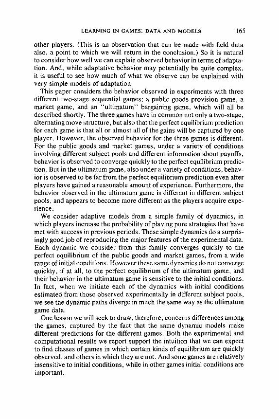
is highlighted by a broader line. The demands which remain with positive probability at round 100,000 are shown by asterisks, and the rejection probabilities which remain positive at round 100,000 are shown by circles.

To make things clear, look at simulation A, represented by the first column of Figure 2a. Consider first the demands of player I. In the very first rounds, the modal demand of player 1 is 5, represented by a single broad dot in row 5. Almost immediately, the modal demand drops to 4, however, represented by the broad line in row 4. In the meantime, the probability that player 1 demands 5 declines quickly to almost zero, while

L E A R N I N G IN G A M E S : D A T A A N D M O D E L S 187

DEMAND Mean

7.5 • o v ~ = m B o o o .~'

5 . ~ e

2.5- PROB

P(9)- ~ , = ~ A ~ , * • . " ."

P(8)- ~ • .2'~i~ '

P ( 7 ) -

P(6)" ~ o •

~/~muk• °'9._ _ k P(5)

P(4)

P(3)

P(2)-

P(1)

t _

0

pm=,.oo t3 "u

d u

0

4" " "

. - ~ "A - - ~ .A

• 0 ' A • • " .' ', " . / "A. ,

& O , L . ". o ." o ~ . . ~ n . 0 I I

i ~ m ~ m B 6 &

.o. ~o.,L,_ ~o._ L --2, ,0 . . . . . . . . . . ~_

- - L . . . . . . . . ~..:.±= i I L ~ Q ¢ _ _

- - : . t : ~ m - " Q ° - - ~ 1 2 9 ; : ~ e . - _

L_ ~ - - -

L

A B C D E

SIMULATION --- ~- : Prob of demand at T = 0 - 1 0 0 -" :- -" Prob of rejection ut T - 0 - 1 0 0 • • • Modal demand e - - e - - e Mean demand o . o • o Demand at T - 1,000, 10,000, 100,000 and 1,000,000 -b . <b • ~ prob of rejection st T = %000, 10,000, 100,000 a n d 1,000,000

FIG, 2--Continued.

the probability that he demands 6 starts to rise, as does the probability that he demands 7. The probability that player 1 demands anything other than 4, 5, 6, or 7 starts low in this simulation, and drops quickly to zero. As we near the end of the 300 trials, the modal demand shifts from 4 to 6, represented by the broad line in row 6. By the end of the 300 trials, the probability that player 1 will demand 4 is still not much below 0.5, but it has dropped almost to zero by the end of 100,000 trials, as indicated by the asterisk in row 4. Similarly, the other demands which still have a positive probability at round I00,000 are 6 and 7, as indicated by the

188

DEMAND

ROTH A N D EREV

e 9"

8"

7"

6-

5"

4"

3"

2.

1

9

o

.." 0.13 ~=,=e~. =.°"

o

MIReII s e ~

o

6

A B C

SIMULATION o . o . o ~ - . 0 1 , ~ - 0 , ~ 0 O.O.O ' F,=O, 1:-.05, 10=0

FIG. 2--Continued.

." OD

/ 6

D E

• O-~.-O. /~mO, ; o .05, ~ i . 0 0 1

asterisks in those rows, and these probabilities have both reached approximately 0.5. The lack of an asterisk in rows 8 and 9 (and in rows 1, 2, 3, and 5) means that the probability that player l will make those demands has dropped to zero by round 100,000, i.e., these demands have been completely extinguished.

Continuing to look at simulation A, note that the probability that player 2 rejects a demand of 8 quickly rises to near 1, as represented by the dotted line in row 8, and at round 100,000 it is very near l, as represented by the open circle. The probability that player 2 will reject a demand of 7 however, has dropped to zero in the very first rounds. This means that, with very high probability, player 2's maximal acceptable demand is 7, but by round 100,000 there is still a small chance that his maximal acceptable demand is 8. In simulation A all of player 2's other strategies have quickly dropped away, but in some of the other simulations the progress of the dotted lines representing player 2's probability of rejecting each demand can be more clearly followed.

Finally, the overall progress of simulation A is reflected in the very top row, which graphs the mean demand of player 1. Notice that this starts around 5, and after an almost imperceptible dip climbs very slowly throughout the first 300 rounds. (So even though the modal demand drops to 4 for many initial rounds, the increasing probability of demands of 5 or 6 keep the mean demand moving up.) By round 100,000, player l 's

LEARNING IN GAMES" DATA AND MODELS 189

mean demand has moved to between 6 and 7. (Note that it cannot go above 7 even as t goes to infinity, since the demands of 8 and 9 have been extinguished, and in the cutoff model extinction is forever . . . . )

Looking now at all 10 simulations, observe that even after 100,000 rounds, the modal demands are mostly between 4 and 6, far from the perfect equilibrium demand of 9. In fact, although the process has not converged in every case by round 100,000, in all ten of these simulations the probability that a demand of 9 or 8 is ever made has been driven to zero, so that convergence must be to a demand no greater than 7. Some simulations do converge to demands of 9, but only rarely: descriptive statistics are given for the cutoff model in Table III. Of the 35 out of 100 simulations that had converged by round 100,000 to a single demand with probability one, only 3 converged to a demand of 9 (while 9 converged to a demand of 6). The picture is similar when we look at the modal demands at t = 100,000 for all 100 simulations in the sample (i.e., including those which have not yet converged to a single demand): only 5 have a modal demand of 9, compared, e.g., to 23 with a modal demand of 6.

Of the 10 simulations shown in Figure 2a, four have actually converged by round I00,000, in the sense that a single demand is made with certainty. These are worth closer examination.

Simulation C converged, after 2090 rounds, to an equilibrium in which player 1 demands 7 with certainty, and player 2 accepts this demand but rejects higher demands with positive probability. 2° Simulation D converged, after 21,723 rounds to an equilibrium at which player 1 demands 6 with certainty and player 2 accepts, but rejects higher demands with high probability (i.e., player 2 sets his maximal acceptable demand at 6 with high probability). Simulation E converged, after 26,865 rounds, to an outcome that is n o t a Nash equilibrium: player 1 is demanding 7, but player 2 would not reject a demand of 8. Simulation I, after 3988 rounds, also converges to an outcome that is not a Nash equilibrium: player 1 is demanding 6 with certainty, but player 2 accepts demands as large as 8 with high probability (although he rejects demands of 9 with certainty), so player 1 could do bet ter by demanding 8. '-I

20 At round 100,000 player 2's probability for setting his maximal acceptable demand to 7 (and hence of rejecting offers of 8 or 9) had declined to 0.11306. (Otherwise his maximal acceptable demand is 9, i.e., he accepts all demands.) Because player 1 converged to demanding 7 with certainty, both of these strategies give player 2 a payoff of 3, so there is no more learning going on, only random drift between m2 = 7 and m2 = 9. Of course, since the cutoff probability/z is positive, either of these may go to zero. By round I00,000 the state of the system has drifted a little out of equilibrium: if player 1 were to demand 8, his expected payoff would be 7.096, i.e., a little more than 7.

2t However, note that both of these non-Nash equilibrium outcomes are consistent with various notions of "self-confirming" equilibria such as those studied by Fudenberg and Levine (1993).

190 ROTH AND EREV

TABLE III

ULTIMATUM GAME WITH RANDOM INITIAL PROPENSITIES

Cutoff model /~ = 0.01, e = 0

Experimentation with forgetting model

/z = 0, e = 0.05, ~ = 0.001

No. of sim with No. No. of sim with Demand the mode converged Mean P the mode Mean P

i 0 0 0.00 0 0.00 2 2 1 0.02 0 0.00 3 4 2 0.05 0 0.00 4 12 3 0.12 0 0.00 5 18 7 0.20 0 0.00 6 23 9 0.22 0 0.03 7 19 8 0.19 8 0.19 8 17 2 0.14 80 0.57 9 5 3 0.05 12 0.21

Sum 100 35 1.00 100 1.00

Local experimentation models (without forgetting) /z = 0, e = 0.1,~o = 0

No. of sim with No. of sim with Demand the mode Mean P the mode Mean P

p. = 0, e = 0.05, ~p = 0

I 0 0.00 0 0.00 2 1 0.01 0 0.01 3 3 0.05 3 0.05 4 8 0.11 I1 0.11 5 22 0.19 19 0.18 6 23 0.23 25 0.23 7 22 0.20 27 0.25 8 15 0.14 11 0.13 9 6 0.06 4 0.05

Sum 100 1.00 100 1.00

Note. Descriptive statistics for 100 simulations at t = 100,000.

To adequately compare the three models for the ultimatum game, we need to carry the simulations out to t = 1,000,000. Figures 2b-2d graph the results for five such simulations, for the cutoff, local experimentation, and experimentation with forgetting models, respectively. Each of the five simulations A through E in these three figures are begun with the same initial propensities (i.e. the randomly generated initial propensities are the same in each of the three simulations labeled A, etc.), so the results of each simulation can be compared for each of the three models. This comparison is easiest to make by looking at the top row of each


figure, which graphs the mean demand. For convenience, the means for all three models are presented together in Fig. 2e, for t = 0-100 and for t = 1000, 10,000, 100,000, and 1,000,000.

For our present purposes, the notable feature of these three models is that they are not very different until t = 10,000, even though their long term behavior is quite different, in that the experimentation model with forgetting converges to the perfect equilibrium demand in all five simulations, while the other two models do not.

The easiest way to see the differences between the models is to focus on simulation D, in which the cutoff model converged to a unique demand of 6, shortly before t = 1000 (at t -- 801). So in Figures 2b and 2e, the cutoff model is flat for simulation D from t = I000 on. In the local experimentation model without forgetting (Fig. 2c) the probability that player 1 will demand 6 starts to decline even before t = 100, although it remains the modal offer at t = 1,000,000. But in the experimentation model with forgetting (Fig. 2d) the probability that the demand will be 6 has dropped to virtually zero by t = 100,000 (at which time the modal demand is 8), and by t = 1,000,000 the modal demand is the perfect equilibrium demand of 9. 22

Table III presents some statistics for 100 simulations out to t = 100,000, for various choices of parameters. It serves to emphasize just how long the long term can be. Note that by t = 100,000 the modal probability is only for a demand of 8 in the forgetting model, although the t = !,000,000 simulations (Fig. 2e) reveal that with high probability this will eventually move to a demand of 9.

So a conventional treatment of these models, which focuses on their asymptotic behavior, would treat the cutoff model and the experimentation with forgetting model as fundamentally different. But their intermediate term behavior is the same, and we will see in what follows that this is what is descriptive of the experimental results.

After all this somewhat complex behavior it is a relief to look at Figs. 3a-3c which each show five market simulations. (Once again, these figures are read vertically, each column corresponding to one simulation.) Each simulation has ten buyers, each of whose initial propensities are randomly drawn (independently) from a uniform distribution as described above, with the same initial propensities being used for all three models. The public announcement of the market price is modeled by having each player update his propensity to play the winning bid after each round. 23 Figures

22 These simulations have e = 0.05. When e = 0.1 the mode for the model with forgetting appears (from a small sample) to be more often at 8 than 9, even at t = 1,000,000.

23 The reinforcement x (equal to the profit from the winning bid) is distributed among the ten players; e.g., if the winning bid is 8, the tendency to play 8 is increased by 2/10 for all players. When the propensities are updated by x (instead of x~ 10), convergence to the perfect equilibrium price is correspondingly faster.

192

PRICE

R O T H A N D E R E V

a

PROB P(9.75)

P(9)

P(8)

P(7)

P(6)

P(5)

P(4)

P(3)

P(2)

P(1),

P(0.25)

f - - f f -

l q NI

: : I I '

. . . . . i . . . . .

A

. . . . . I . . . . . . . . . . I . . . . .

B C

SIMULATION

7 7 1 1

i '

e • : 7 7 7 :

J

. . . . . i . . . . . i . . . . .

D E

: : ; Prob of stating the price

FIG. 3. M a r k e t g a m e : F i v e s i m u l a t i o n s wi th r a n d o m ini t ial v a l u e s . T = 0 - 3 0 0 ( e v e r y 20),

o n e g a m e p e r r o u n d , c o m m o n l e a r n i n g . (a) S( I ) = 10, e = 0, p. = 0 .01 , ~ = 0. (b) S ( I ) =

10, e = 0 . 0 5 , / z = 0, ~p = 0. (c) S( I ) = 10, e = 0 . 0 5 , / x = 0, ~p = 0 .001 .

3a-3c graph the average probability over the I0 buyers that an individual buyer will state each of his feasible bids. (So this is a measure of individual behavior, not merely of market behavior as we would get by graphing the probability for the maximum bid.) As the figures show, this probability quickly goes to 1 for the highest feasible bid, and zero for all the other bids, using either the cutoff or local experimentation models.

These simulations show that the three games have different properties, which shows up early in the simulations, even using dynamic models with different long term behavior. What these simulations do not do is model

PRICE


b PROB'

P(9.75) '

p(8)i P(7):

P(6):

P(5) I

P(4) I

P(3)

P(2)

P(1)

P(0.25)

S r.---

: 771 I

I

7 :11 I I

: : : : : i l l

1

. . . . . = . . . . . . . . . . i . . . . . . . . . . = . . . . .

B 13 D

SIMULATION : : --'- P rob o f tnadng the price

A E

FtG. 3--Continued.

the experimental environments discussed in Section II, because these simulations do not model the manner in which a population of experimental subjects gained experience with changing partners, nor do these simulations model the initial conditions observed in the experiments. Since these simulations do show that the ultimatum game in particular is sensitive to the initial conditions, this is likely to be important. We address these issues next.

194

PRICE

ROTH AND EREV

C

PROB, P(9.75) '

P(8) '.

P(7) '.

P(6) I

P(5) I

P(411 P(3) I

P(2) I

P(1) I

P(0,2B) I

f - f - f - f -

A

- - 7 . . . . . . . . .

B C D E

SIMULATION : : : P rob of stating ~e price

FIG. 3--Continued.

VI. SIMULATION OF THE EXPERIMENTS

Here we describe simulations which model the experimental environments in which the data discussed in Section II were collected. We first describe how the initial propensities to play each pure strategy of the simplified games described in Section IV were estimated from the data. Separate estimations are carried out for each cell of the experiments, i.e., for the ultimatum and market games in each of four countries, and for


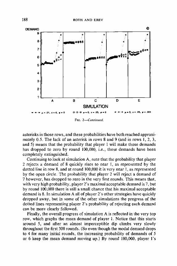
the best shot game in each of two information conditions. We begin with a description of how the initial conditions were estimated for the ultimatum game, which the results of the previous section suggest is the game which will be most sensitive to the estimates of initial propensities.

The Ultimatum Game. Each of the observed player 1 demands in the first two rounds was first transformed into the closest demand in the simplified game (an integer from 1 to 9). When two values were equally close the lower one was chosen (i.e., 0.5 was rounded downward). The initial propensity (IP) to follow each strategy was computed as the relative frequency of the transformed demands, which are tabulated in the appendix. For example, if 6 of the 60 demands were in the range [5.5, 6.5) the IP of 6 was set to be 6/60 = .I.

To assess the initial propensities of player 2 the proportion of rejections of each of the nine demands was first computed. Under the assumption that player 2's strategies are of the form "accept a demand of no more than m" these proportions should not decrease as the demands increase. As can be seen jn the appendix, violations of this assumption were observed in only 6 of the 32 cases (8 (increase) x 4 (countries)). In order to compute the IP, it was assumed that these violations reflect random error and monotonicity was restored by "pooling" categories. For example, if4 of 6 demands of "8" were rejected and only 2 of 4 demands of "9" were rejected, the rejection rates in those two categories were replaced by a pooled estimate of 0.6 -- (4 + 2)/(6 + 4). The six monotonicity corrections are also presented in the appendix.

Once monotonicity was restored the calculation of the initial propensities is straightforward. If the corrected rejection rate of demand i is R(i), the estimated tendency to follow a strategy that accepts i, but rejects higher demands is IP (m = i) = R(i + 1) - R(i).

The Market Game. Buyers' bids were treated precisely as player 1 demands in the ultimatum game. Each of the observed prices in the first two rounds was transformed into the closest price in the simplified game (with upward rounding--see the appendix). IPs were assessed by the relative frequencies. As noted earlier, no rejections by sellers were observed.

The Best Shot Game. For the best shot game we had the smallest number of observations, but the largest number of possible strategies. To reduce the number of strategies for which there are no observations, observations that fell between two strategies were divided between the two. Player l 's observed choices (ofq~ = 0, I, 2, 3, or 4) in the first two rounds of the experiment were transformed into the closest demand in the simplified game (q i = 0, 2, or 4), by counting intermediate observations as half an observation each for the simplified strategies (i.e., an observation

196 ROTH AND EREV

of q~ = 1 is counted as half an observation each of ql = 0 and q~ = 2) and the IPs were estimated by the relative frequencies. For player 2, the probabilities of each of the possible responses (q2 = 0, 2, or 4) were first calculated from the simplified player I behavior in the first two rounds of the experiment. Then, the probability of each of the 27 response rule triples (response to q t = 0 with x, to q~ = 2 with y, and to q~ = 4 with z) was estimated to be P(xyz) = P(x[O)P(y[2)P(z[4) (see the Appendix).

The simulations were modeled on the experiments, so that in each best shot simulation there are ten player I 's and ten player 2's. In each round of each simulation, ten games are played, each one pairing one of the player l 's against one of the player 2's, and from round to round the pairings change, so that after ten rounds each player 1 has played each player 2. In the full information simulations, each player 1 starts with the (same) initial propensities estimated from the data for players 1, and each player 2 starts with the initial propensities estimated for players 2. Similarly in the partial information simulations, the players 1 and 2 each start with the propensities estimated from that data set.

Figure 4 shows representative results for the best shot game. The first two columns summarize the experimental data observed in Prasnikar and Roth (1992), while the next two columns graphs the average of one hundred simulations with parameters/x = 0, e = 0.05, and ~o = 0.001, for times t = 0, 10, and I00 (i.e., for substantially more than the 10 rounds actually observed in the experiments). Both the experimental data and the simulation results are presented in terms of the simplified game, so that, in particular, the simulations in each information condition are initialized from the corresponding data as shown in the figure.

Table IV displays the results of 100 simulations for each of the three models, for both the full and partial information conditions. As the table shows, the three models are virtually identical at both t = 10 and t = 100. (The simulations with e = 0.1 are very similar.)

Looking first at the Full Information simulations, note that even after only ten rounds, the probability that player 1 will choose the perfect equilibrium quantity qj = 0 is just about 80%, while the probability that player 2 will respond to q~ = 0 with the perfect equilibrium response of q2 = 4 is slightly over 50%. Thus the simulations are strikingly close to the experimental data in real time, i.e., in I0 periods. By t = 100 the simulations have moved still closer to perfect equilibrium, with player 2's response moving more slowly than player I 's , for the reasons discussed earlier.

The Partial Information simulation results are also comparable to the experimental results in real time. At t = I0 the probability is over 50% that player 1 will play the perfect equilibrium, and not quite 20% that player 2 will make the perfect equilibrium response. By t = I00 player 1



q = 4 . 1

q = 2 1

q = 0 1

\

S 4"

. . u

) . " 0 . . . . . . . . 0 . . . . . . . . 0

\ O'

4 "='

0 ' : : , : 0 4' '=

i i

FULL PARTIAL

EXPERIMENTAL DATA

. . . 0

0 . . . . . . 0 " "

4 . . . . . . 4 . . . . . . . . 4

i i . . . . . . . . 4 • '

. . . . . . . 2 2

" 0 . .

' • 0

: -~ - - P rob their I p rov ld lm th l l l a r r l oun t • IZ. • R. P rob t ha t II r esponds w i t h 2

. . . . . 0 . . . . . . . . 0

8 . . . . . . . . 0 . . . . . . 0

• . . . . • 2

. . .

, , . ' .~ . 4 • .

i i

FULL PARTIAL

SIMULATION RESULTS 0 • 0 • O' p r o b tha t II respor lds w i t h 0 4 • 4 • 4" P rob thSt II r e s p o n d s w l t l l 4

FIG. 4. Best shot: Experimental data and simulations (initialized from the data), t = 1 and 2, 9 and 10 (in the experiment); T = 0, 10, 100 (in the simulation). S(I) --- 10, e = 0.05, /x = 0, ~p = 0.001

has moved very much closer to perfect equilibrium, while player 2 is learning much more slowly.

Comparing the Full and Partial Information conditions, we see that in the simulations, just as in the experimental data, the full information condition moves towards perfect equilibrium more quickly than the partial information condition. This makes plausible the hypothesis that, in the experiments as in the simulations, the effect of letting the players know

198 ROTH AND EREV

TABLE IV

BEST SHOT GAME WITH INITIAL PROPENSITIES ESTIMATED FROM THE DATA

Model

t ~ = 0.01 e = 0.05 e = 0.05, ~ = 0.001

Full information Player I: Mean and median values of P(player I chooses q~ = 0)

Mean 10 100

I000 Median 10

100 1000

Player 2 :Mean and median values Mean 10

100 1000

Median 10 100

1000

Player 1: Mean and median values Mean 10

100 1000

Median 10 100

1000

Player 2: Mean and median values Mean 10

100 I000

Median 10 100

1000

0.80 0.78 0.78 0.96 0.93 0.93 1.00 0.96 0.97 0.81 0.79 0.79 0.97 0.93 0.93 1.00 0.96 0.97

of P(player 2 chooses q2 = 4 ] ql = 0) 0.56 0.55 0.55 0.67 0.63 0.64 0.78 0.74 0.77 0.56 0.55 0.56 0.67 0.69 0.65 0.78 0.74 0.78

Partial information of P(player 1 chooses ql = 0) 0.53 0.51 0.52 0.88 0.85 0.86 0.99 0.95 0.96 0.53 0.51 0.53 0.88 0.85 0.87 0.99 0.96 0.96

of P(player 2 chooses q2 = 4 ] q l = 0) 0.16 0.17 0.18 0.19 0.20 0.21 0.29 0.30 0.36 0.15 0.17 0.17 0.19 0.19 0.20 0.28 0.31 0.36

Note. Descriptive statistics for 100 simulations at t = 10, t = 100, and t = 1000.

each others ' payoffs is felt primarily in the first period, after which similar adaptive behavior is observed.

Figure 5 shows results for the ultimatum game. The first four columns summarize the experimental data observed in Roth et al. (1991), while the next four columns graph the average of one hundred simulations with parameters /x = 0, e = 0.05, and ~o -- 0.001, for times t = 0, 10, and 100.

In the ultimatum game simulations there are also ten player l ' s and ten

L E A R N I N G I N G A M E S : D A T A A N D M O D E L S 199

DEMAND PROB-

P(9)

P(8)

PC-/)

k.

"n

k ,o

I"-.,i ' >, ,_.

_" g.

j - + --.o....ll~ /

k,....&.... A ~'"O-...& +'"l~-.0.&

+-,.~ I... ".- "-Ik....A ~'"A--.- d

P(6) ¢+~ ~ ~ . ~ ~ ~ ~

P(5) --o ,--4 ~ ~ ~ ~

P(4)

P(3)

&

P(2)

P(1)

= : = " - = : : - r . : " " - : - - : = - _ - : "

ISR JAP USA SLO ISR JAP USA SLO

EXPERIMENTAL D A T A SIMULATION RESULTS

Demand .,~-~...-A. prob of rejection • • • Modal demand

F I G . 5. Ultimatum: Experimental data and simulations (initialized from the data). T = 1

and 2, 9 a n d 10 (in the experiment); T = 0, 10, 100 (in the simulation). S ( I ) = 10, e = 0 . 0 5 ,

/x = 0, ~p = 0 . 0 0 1 .

player 2's. In each round, 10 games are played, each one pairing one of the player l's against one of the player 2's, and from round to round the pairings change, so that after 10 rounds each player 1 has played each player 2. In each of the country simulations, each player 1 starts with the (same) initial propensities estimated from the data for players 1, and each player 2 starts with the initial propensities estimated for players 2 for that country.

200 R O T H A N D E R E V

T A B L E V

U L T I M A T U M GAME WITH INITIAL PROPENSITIES ESTIMATED FROM THE DATA

Mean demand

Mean probability Probability of simulation with

t = 10 t = 100 t = 1000 mode above 5 Med. move t = 10 100 1000 P(5) P(6) P(5) P(6) P(5) P(6) t = 10 100 1000

Cutoff model: S(I) = 10, e = 0,/,t = 0.01, qJ = 0 Israel 3.5 5.47 5.63 5.83 0.37 0.28 0.39 0.36 0.39 0.40 0.47 0.63 0.83 Japan >1000 5.13 5.17 5.29 0.34 0.22 0.43 0.26 0.46 0.27 0.13 0.17 0.28 U.S.A. >1000 5.09 5.25 5.45 0.50 0.28 0.53 0.31 0.53 0.33 0.09 0.25 0.45 Slovenia >1000 5.00 5.01 5.12 0.60 0.20 0.61 0.24 0.62 0.25 0.00 0.01 0.12

Local experimentation model: S(I) = 10, e = 0.05, p. = 0, qJ = 0 Israel 4.0 5.49 5.71 5.92 0.37 0.35 0.34 0.41 0.29 0.46 0.49 0.71 0.91 Japan >1000 5.16 5.20 5.42 0.40 0.26 0.41 0.31 0.39 0.36 0.16 0.20 0.42 U.S.A. 510.0 5.10 5.32 5.55 0.49 0.31 0.45 0.35 0.39 0.40 0.10 0.32 0.55 Slovenia >1000 5.01 5.05 5.25 0.58 0.24 0.53 0.30 0.47 0.37 0.01 0.05 0.25

Experimentation model with forgetting: S(I) = 10, e = 0.05, ~ = 0, ~b = 0.001 Israel 4.0 5.49 5.71 5.95 0.37 0.35 0.34 0.41 0.28 0.46 0.49 0.71 0.94 Japan 626.5 5.16 5.21 5.53 0.40 0.26 0.41 0.31 0.38 0.37 0.16 0.21 0.52 U.S.A. 428.5 5.10 5.32 5.64 0.49 0.31 0.45 0.36 0.38 0.41 0.10 0.32 0.64 Slovenia >1000 5.01 5.05 5.31 0.58 0.24 0.53 0.30 0.46 0.39 0.01 0.05 0.31

Note. Descriptive statistics for 100 simulations at t = 10, t = 100, and t = 1000.

Table V presents mean results of I00 simulations of each of the three models, starting from the initial propensities estimated for each country, at times t = 10, t = I00, and t = 1000. Recall that at round 1 the modal demand in every country was 5, and in the experimental data it had moved by round 10 to a modal demand of 6 in Israel, to modal demands of 5.5 and 6 in Japan, but remained at a modal demand of 5 in the U.S. and Slovenia. The first column of numbers (labeled MedMove) reports the median round in which the modal demand moved from 5 to 6 in the simulations. In each of the three models the modal demand in the Israeli simulations moved from 5 to 6 in real time (on average by round 4), while the Slovenian simulations remained at a mode of 5 through time t = 1000. The modal demands in the Japanese and US simulations sometimes moved from 5 to 6 in the intermediate term, but were sensitive to the path of play in each simulation. Each of the other descriptive measures preserves the relationship that demands decline as we move from Israel to Slovenia, with Japan and the U.S. in between. For example, at t = 10 the mean demands in the cutoff model simulations decline from 5.47 for Israel to 5.00 for Slovenia, while the probability that a player 1 will demand 6 declines from 0.28 to 0.20, and the probability of a simulation in which the modal demand is above 5 declines from 0.47 to 0.00. Notice that the forgetting model, which we have seen moves much closer to the perfect equilibrium than the local experimentation model in the long term, never-


PRICE PROB'

'<"=/ / / J S J S

P(8

P(7

P(6

P(5

P(4 L _

P(3

P(2 L ~

P(1)

L C v - - Ig - =

m m ~ ~ .

P(.25)

ISR J A P U S A S L O I S R J A P U S A S L O

EXPERIMENTAL DATA SIMULATION RESULTS -~- ~ ¢- Prob of stating ~ e p d c e

FIG. 6. Market game: Experimental data and simulations (initialized from the data). T = 1 and 2, 9 and 10 (in the experiment); T = 0, 10, 100 (in the simulation). S(I) = 10, e = 0.05, p. = 0, ~0 = 0.001.

theless yields very similar predictions in the intermediate term. And it is the intermediate term results (for each of the models) that track the experimental data well.

Note also that the results of the ultimatum game simulations initiated with data from the four countries are quite different in the intermediate term from those initiated with random propensities. Thus the observed initial behaviors were not random, but reflected something of the players'

202 ROTH A N D EREV

T A B L E VI

MARKET GAME WITH INITIAL PROPENSITIES ESTIMATED FROM THE DATA

t = 10 t = 100

P(8) P(9) P(9.75) P(SPE) P(9.75) P(SPE)

Cutoff model: e = 0, p. = 0.01, $ = 0 Israel 0.18 0.30 Japan 0.22 0.29 U.S.A. 0.20 0.24 Slovenia 0.28 0.24

Local experimentation model: e = 0.05, Israel 0.18 0.31 Japan 0.22 0.29 U.S .A. 0.20 0.24 SIovenia 0.28 0.25

Local experimentation model with forgetting: Israel 0.18 0.31 0.38 Japan 0.22 0.29 0.26 U.S.A. 0.20 0.24 0.08 Slovenia 0.28 0.25 0.18

1.00 0.79 1.00 0.14 0.75 1.00 0.00 0.69 1.00 0.00 0.71 1.00

0.38 0.26 0.09 0.19

t~ = 0,~0 = 0 0.38 1.00 0.76 1.00 0.26 0.07 0.72 1.00 0.08 0.00 0.65 1.00 0.18 0.00 0.69 1.00

e = 0.05, p, = 0, ~ = 0.001 1.00 0.77 1.00 0.23 0.73 1.00 0.00 0.67 1.00 0.00 0.70 1.00

Note. Descriptive statistics for 100 simulations at t = 10 and t = 100. probability that an individual buyer bids x. P(SPE) equals the probability price is 9.75.

P(x) equals the that the modal

perceptions of the game--perceptions that were different in the different countries.

Figure 6 shows results for the market game. The first four columns summarize the experimental data observed in Roth et al. (1991), while the next four columns graphs the average of one hundred simulations with parameters/z = 0, e = 0.05, and ~p = 0.001, for times t = 0, 10, and 100. In the market simulations, as in the experiments, two markets were run simultaneously, with changing sets of buyers. There were ten buyers in each market simulation, and in each country condition all buyers had the same initial propensities, as estimated from the data. z4 Consistent with the results of the random simulations, the different initial propensities have no lasting effect. Table VI gives statistics from 100 simulations, for each of the three models. In each country simulation, each bidder quickly

24 To model the fact that in the experiment all subjects learned the winning bid in both of the markets, in the simulations there were two reinforcements (to the two winning bids) distr ibuted among the 20 players. If, for example , the winning bids were 9 in market A and 9.75 in market B, the propensity to play 9 is increased by 1/20, and the propensity to play 9.75 is increased by 0.25/20 for all players.


converges to bidding the perfect equilibrium price with high probability. And the models track the data reasonably well in real time, i.e., by t = 10, while by t = 100 the simulations have converged almost completely to perfect equilibrium behavior.

VII. CONCLUSIONS

The substantive results of this paper are easy enough to summarize. Independently of the experimental data, the simulation results starting from random initial propensities reveal a structural difference between the ultimatum game and the other two games. And in comparison with the experimental data, the intermediate term predictions of both the cutoff model and the local experimentation models track the major experimental observations well. Despite the different long term behavior of these dynamic models, their intermediate term predictions agree with the experimental data in that:

1. In the maFket and best shot games, both predicted and observed behavior quickly approach perfect equilibrium play, but in the ultimatum game neither predicted nor observed behavior approaches perfect equilibrium.

2. Both predicted and observed behavior approach perfect equilibrium play more quickly in the best shot game with full information (in which the experimental subjects knew one another's payoffs) than in the best shot game with partial information (in which the experimental subjects knew only their own payoffs).

3. Both predicted and observed behavior in the ultimatum games (but not in the market or best shot games) are different in the different countries sampled, and the predicted intermediate term differences track the observed differences (within the limitations of the simplified games).

These results indicate that even very simple adaptive models may be quite useful both for distinguishing which games are likely to be sensitive to initial conditions and for predicting how initial conditions matter. 25

,2 And while it seems clear that much of the progress to be made in understanding learning in games will come on the interface of economics and psychology, the fact that there are some games which exhibit both predicted and observed behavior that seems not to be sensitive either to initial conditions or subject pools suggests that there is also substantial progress to be made by understanding which classes of games fall into this category. That is, there appear to be classes of games for which it will turn out that the observed learning behavior is primarily a property of the game, rather than of the particular learning processes used by the players. (This is the traditional economists' viewpoint, but similar views have begun to emerge among cognitive psychologists. See in particular Anderson (1990), who argues that in many cases the best available predictions about mental processes come from an understanding of the structure of the environment.)

204 ROTH AND EREV

Recall that the adaptive models studied here do not model in any way what players know about the game, or believe about the future behavior of other players. That such simple dynamic models, when initiated with first period observed behavior, nevertheless do a good job of predicting how observed behavior will evolve, suggests that a substantial part of how players' knowledge and beliefs influence the game may be reflected already in first round data. For example, the data from the two information conditions of the best shot game suggest that players' behavior in that game approaches perfect equilibrium faster when they know each others' payoffs. But the simulation results suggest that the effect of this knowledge may be primarily to alter the first period behavior, and that the ways in which players adapt in subsequent periods to their experience may be similar in both information conditions. The same can be said about the between-country differences in the ultimatum game data. It could be that these differences result from different perceptions (of the game, and of their countrymen) held by players in different countries, or it could be that they result from different patterns of adaptation. That the same dynamic model can track the between-country differences when initiated from the first round data lends support to the former hypothesis.

Of course the comments of the previous paragraph are still somewhat speculative, based as they are on a relatively small data set arising from only three kinds of games. Preliminary indications are that the correspon- dence between predicted and observed behavior may survive the transition to larger data sets and different kinds of games. We hope to report on both some successes and failures of this simple model in a future paper.

To speculate a little on theoretical matters, there are reasons to think that these results will also be robust to the choice of dynamics, so that very different dynamic models might produce similar results. The family of models we have considered are driven in the early rounds by the payoff differences among strategies, based on the initial propensities to play each strategy. For example, the reason that behavior in the ultimatum game remains distant from the perfect equilibrium is that the propensity to make very high demands falls more quickly than the propensity to accept very high demands rises. This is because the difference between accepting and rejecting a very high demand is small and thus has only modest impact on the propensities of players 2, while the difference for players 1 between having a very high demand rejected, and earning zero, or having a moderately high demand accepted, and consequently earning more than half the pie, is much larger, and more quickly increases the propensity to make only moderately high demands. Once players 1 seldom make very high demands, there is even less pressure on players 2 to learn not to reject them, and s o o n . 26

26 A similar conclusion about ultimatum games is reached by Gale et al. (1995), using a model of evolutionary dynamics.


Note also that there are good reasons to think that the actual learning rules (or even the strategies) used by the subjects in the experiments differ in important ways from our simple models, and that this too supports the conjectured robustness of the results. 27 That the simple simulated learning rules may be very different from those used by the experimental subjects, but both sets of rules produce similar intermediate term outcomes, suggests that very different learning rules will quickly approach perfect equilibrium in the best shot and market games, but not in the ultimatum game.

Methodologically, an important difference between this paper and most of the recent theoretical literature on game dynamics is our concern with intermediate term results, rather than asymptotic convergence. Although we have not attempted to define the "intermediate term" any more precisely than to say that it starts when the learning curve flattens out, this has not proved to be a problem in looking at the simulated behavior we report, precisely because the learning curves soon become very flat in- deed. For the dynamics considered here, the intermediate term starts in the tens of iterations, and, at least in the ultimatum game, does not give way to the sometimes very different long term predictions for thousands or even hundreds of thousands. Of course these numbers will be different for different dynamics. 28 To the extent that intermediate term behavior of dynamic models is important, it may be useful for theorists to pay more attention to the entire vector field generated by a dynamic, and not just to its limit points and basins of attraction. 29

27 Particularly in repeated games, the set of strategies possibly available to the players may be enormous. The traditional posture of game theory has been to regard all possible strategies as available, but just as players may not be hyperrational in other respects, their capacity to consider a vast number of strategies may also be limited. (One attempt to deal with this has been to represent the strategies available to a player in a repeated game as those which can be implemented by finite state automata of limited size. An early example of this approach can be found in Tsetlin, 1973. Before his untimely death in 1966, he developed interesting models of learning in repeated games, with players modeled as automata.) Research in psychology has often identified particular strategies which may occur with high initial propensities. For example, in repeated experiments with T mazes, rats have an initial propensity to follow an alternation strategy (i.e., not to choose the same leg of the maze twice in succession); see, e.g., Dember and Fowler (1958). We anticipate that the accuracy of predictions of models like those considered in this paper may be improved by assessing the repeated game strategies the subjects employ.

28 For our present purposes, the very slow convergence of the models without forgetting only serves to emphasize the difference between the ultimatum game and the other two games (in which all three models nevertheless converge quickly). For more extended study of games with very slow convergence properties it will likely be desirable to consider faster converging dynamics, e.g., by having a positive forgetting parameter, or some other way of keeping the strengths of the propensities from growing without bound. This has the effect of giving more weight to recent events, instead of weighting all payoffs equally whenever they occur, as in our models without forgetting. (The flat learning curves come about because after a while there are so many more past events than recent ones.)

29 More generally, new tools may be required, since for stochastic learning rules understanding the intermediate term means examining the transient phase of a stochastic process,

206 ROTH AND EREV

To bring together our conclusions about games and about models, recall once again that the three games considered here have similar equilibria: in the ultimatum and market games all prices can be supported by some Nash equilibrium, but only extreme outcomes, in which all the wealth accrues to one side, can be supported by a perfect equilibrium. Similarly, the perfect equilibrium of the best shot game yields extreme payoff differences. The experimental results of Roth et al. (1991) and Prasnikar and Roth (1992) show that this similarity of equilibria does not produce similarity of behavior: only in two of the games did observed behavior approach the perfect equilibrium. To the extent that equilibrium is reached, if at all, through a dynamic adjustment process that begins out of equilibrium, the possibility of dissimilar behavior seems natural, since games with similar equilibria may be quite dis-similar out of equilibrium. The present paper further shows that the path of the dynamic process may also be insufficient to predict behavior if its velocity is not also taken into account. This is clearest in our model with experimentation and forgetting, whose predictions approach perfect equilibrium eventually (e.g., by t = 1,000,000) for all three games, but whose rates of change become very low much earlier (e.g. by t = 100). It is the real (t = 10) or intermediate term (e.g. t = 100) predictions which correspond to the observed behavior, both when these predictions are close to the perfect equilibrium and when they are not (and both in the models whose intermediate term predictions are close to their long term predictions and those in which they are not).

That being the case, the reasons for our concern with real time and intermediate term predictions (in contrast to asymptotic predictions) for both field and experimental data are worth restating.

First, we believe that much of the economic phenomena we observe in the world is intermediate term in nature. Although we have concentrated here on demonstrating this for a body of experimental data, it is not only in experiments that long term behavior may be difficult to observe. For example, none of the annual labor markets and matching processes whose historical evolution is studied in Roth (1984, 1990, 1991), Mongell and Roth (1991), and Roth and Xing (1994) have gone for more than fifty years--i .e. 50 iterations--without a change of environment substantial enough to mean that the same game was no longer being played. After such a change the behavior of participants typically goes through a period of readjustments as they adapt both to the new environment and to the new strategies of other agents.

Second, even when we identify economic phenomena with sufficient longevity and stationarity so that it is reasonable to believe they are

A recent monograph on adaptive algorithms (Benveniste et al., 1990) devotes an extremely short section to the subject, which we quote in its entirety (Section 1.4.2, The Transient Phase, p. 30): "Alas! As will be seen, there is very little to say."


yielding long term behavior, there is reason to be cautious about the long term behavior of any models we create. This is because every model includes some elements of the situation being modeled while ignoring others. And when the learning curve becomes flat, there is room for unmodeled factors to become important--factors that may be present at every stage of the learning process, but are unimportant when the learning curve is steep.

To extend the geological analogy used in the introduction, erosion is not the only force that acts on coastlines. If we can expect volcanic eruptions every millenium or two, then, if erosion is slow, this will change our predictions about whether all coastlines will be sandy beaches. And there are also gentle but steady forces such as sedimentation, that work in the opposite direction from erosion, so that when erosion is fast we may be able to neglect them, but when it is slow, they may cause coastlines to rise rather than fall. So the reasons for devoting more attention to intermediate term results are not only that we live and die in the intermediate term and that changes in the environment (including the players) make data for the very long term hard to gather, but also that we have less reason to be confident in a particular model of learning when the learning curve is fiat than when it is steep. Our results here suggest, however, that such models may have considerable predictive power when the learning curve is steep.

In conclusion, this paper reports an exercise in " low" (rationality) game theory. Low game theory differs from traditional, "high" game theory in how the players are modeled: Where high game theory models the players as hyperrational, we have modeled them as simple adaptive learners. 3° What low game theory has in common with high game theory, which distinguishes both approaches from nongame-theoretic models, is the cen- tral place given to modeling the strategic environment, i.e., to the game itself. But here too, there is room to consider the cognitive capacities of the players, since the full strategy sets in a repeated or multiperiod game quickly become large. Although the players in the experiments discussed here were engaged in multiperiod games, we have modeled their strategies by (discretized subsets of) their stage game strategies. This has proved to be sufficient, perhaps because they are not engaged in repeated games (i.e., against the same opponent). However, it is likely that future research in low game theory will have to, at least sometimes, pay close attention to what subsets of very large strategy sets are accessible to and employed by the players.

3o Of course we have chosen one of very many possible ways to model less-than-complete rationality, and the question of what are the best ways will be empirical. (The equilibrium refinement literature shows that there are also a multitude of ways to model hyperrationality.)

208 ROTH AND EREV

M o s t o f the t h e o r e t i c a l r e s e a r c h on a d a p t i v e m o d e l s has f o c u s e d on f inding c o n d i t i o n s u n d e r w h i c h the a d a p t i v e m o d e l s c o n v e r g e to equi l ib- r ium as t ime goes to infini ty. (Thus high g a m e t h e o r y can s o m e t i m e s a r i se f rom low g a m e t h e o r y . ) In con t r a s t , we have a rgued tha t , when the o b j e c t is to d e v e l o p low g a m e t h e o r y in d i r ec t i ons useful for emp i r i ca l e c o n o m i c s , infinite t ime ho r i zons d e s e r v e to be t r e a t ed wi th the s ame s k e p t i c i s m as o t h e r idea l i za t ions . N e v e r t h e l e s s , we have seen (in the bes t sho t and m a r k e t games ) tha t for s o m e g a m e s the i n t e r m e d i a t e t e rm p r e d i c t i o n s o f low g a m e t h e o r y c o r r e s p o n d with t h o s e o f high g a m e t he o ry . W e c on j e c - ture tha t , w h e n they c o i n c i d e , the c o m m o n p r e d i c t i o n s o f bo th k inds o f g a m e t h e o r y will qui te gene ra l l y p r o v e to be r o b u s t l y d e s c r i p t i v e o f ob- s e r v e d b e h a v i o r , as t hey we re here . F o r o t h e r g a m e s , l ike the u l t i m a t u m g a m e , the p r e d i c t i o n s o f low and high game t h e o r y d ive rge . W e have s h o w n he re tha t (even) in such cases ) , the p r e d i c t i o n s o f low g a m e t h e o r y m a y be o f i n d e p e n d e n t in t e re s t , b e c a u s e they are d e s c r i p t i v e o f o b s e r v e d b e h a v i o r .

APPENDIX

Data and Initial Propensities for the Ultimatum Game Simulations by Countl~y

Demand

l 2 3 4 5 6 7 8 9 Total

Israel No of demands 0 0 0 l 22 17 7 6 7 60 Player l 's IP 0 0 0 0.02 0.37 0.28 0.12 0.10 0.12 1 No. of rejections 0 2 1 3 3 5 14 Rej. rate: 0 0.09 0.06 0 .43 0.50 0.72 Mon. correction 0.08 0.08 Player 2's IP 0 0 0 0.08 0 0.35 0.07 0.22 0.28 1

Japan No. of demands 4 0 2 3 20 13 7 4 5 58 Player l 's IP 0.07 0 0 .03 0.05 0.34 0.22 0.12 0.07 0.09 1 No. of rejections 0 - - 0 2 2 4 4 3 3 18 Rej. rate 0 0 0 0.67 0.10 0.31 0.57 0 .75 0.60 Mon. correction 0.17 0.17 0.67 0.67 Player 2's IP 0 0 0.17 0 0.14 0.26 0.10 0 0.33 1

USA No. of demands 0 0 2 4 27 15 3 2 I 54 Players I's IP 0 0 0.04 0.07 0.50 0.28 0.06 0.04 0.02 1 No. of rejections - - - - 0 0 5 4 2 I 0 Rej. rate - - - - 0 0.25 0.18 0.27 0.67 0.50 0 Mon. correction 0.19 0.19 0.50 0.50 0.50 Player 2's IP 0 0 0.19 0 0.08 0.23 0 0 0.50 1

APPENDIX--Continued

Demand

1 2 3 4 5 6 7 8 9 Total

Slovenia No. of demands 0 0 0 3 36 12 8 1 0 60 Player l ' s IP 0 0 0 0.05 0.60 0.20 0.13 0.02 0 1 No. of rejections 0 7 2 4 1 - - Rej. rate 0 0.19 0.17 0.50 1 - - Mon. correct ion 0.19 0.19 Player 2 ' s IP 0 0 0 0.19 0 0.31 0.50 0 0 1

Data and Initial Propensities for the Best Shot Game: Number of Obseroations in Each of the Simplified Game's Nine Contingencies in

the First Two Rounds

Condition: Full Partial Quanti ty: q2 q2

0 • 2 4 Sum 0 2 4 Sum

0 1.5 3 5 9.5 2 2 2 6 ql 2 1.5 0.5 1 3 4.25 0.75 0 5

4 3 0 0.5 3.5 5.75 0.75 0.5 7 Sum 6 3.5 6.5 16 12 3.5 2.5 18

Calculation of player l ' s IP 0 9.5/16 = .59 6/18 = .33 2 3/16 = .19 5/18 = .28 4 3.5/16 = .22 7/18 = .39

Calculation of player 2 's IP (a few examples) 000 (1.5/9.5)(1.5/3)(3/3.5) = 0.07 002 (1.5/9.5)(1.5/3)(0/3.5) = 0 004 (1.5/9.5)(1.5/3)(0.5/3.5) = 0.01 020 (1.5/9.5)(0.5/3)(3/3.5) = 0.02 and so forth . . .

(2/6)(4.25/5)(5.75/7) = 0.23 (2/6)(4.25/5)(0.75/7) = 0.03 (2/6)(4.25/5)(0.5/7) = 0.02 (2/6)(0.75/5)(5.75/7) = 0.04

The Market Game: Number of Bids in the First Two Rounds, by Country

Bid

0.25 1 2 3 4 5 6 7 8 9 9.75

Count ry Israel 0 1 0 0 0 2 4 5 16 27 17 Japan 1 1 0 0 1 4 4 10 19 24 8 USA 0 4 I 2 2 14 6 6 14 14 l Slovenia 0 0 0 0 l 3 5 16 24 19 4

209

210 RUTH AND EREV

REFERENCES

ANDERSON, J. R. (1990). The Adaptive Character of Thought, Hillsdale, N J, Erlbaum. AOYAGI, M. (1992). "Evolution of Beliefs and the Nash Equilibrium of Normal Form

Games," mimeo. ARTHUR, W. B. (1991). "Designing Economic Agents that Act Like Human Agents: A

Behavioral Approach to Bounded Rationality," Amer. Econ. Rev. Papers Proc. 81, May, 353-359.

ARTHUR, W. B. (1993). "On Designing Economic Agents that Behave Like Human Agents," J. Evolut. Econ. 3, 1-22.

BENVENISTE, A., METIVIER, M. AND PRIOURET, P. (1990), Adaptive Algorithms andStochas- tic Approximations. Berlin, Springer. [translated from the French by Stephen Wilson]

B[NMORE, K. G., AND SAMUELSON, L. (1993). "Muddling Through: Noisy Equilibrium Selection," preliminary draft.

BLACKBURN, J. M. (1936). "Acquisition of Skill: An Analysis of Learning Curves," IHRB Report No. 73.

BOLTON, G. (1991). "A Comparative Model of Bargaining: Theory and Evidence," Amer. Econ. Rev. 81, December, I096-1136.

BUSH, R., AND MOSTELLER, F. (1955). Stochastic Models for Learning. New York, Wiley. CRAWFORD, V. P. (1991). "An 'Evolutionary' Interpretation of Van Huyck, Battalio, and

Beil's Experimental Results on Coordination," Games Econ. Behav. 3, 25-59. CRAWFORD, V. P. (1992). "Adaptive Dynamics in Coordination Games," working paper,

University of California, San Diego.

CROSS, J. G. (1983). A Theol~y of Adaptive Economic Behavior. New York/London Cam- bridge Univ. Press.

DEMBER, W. N., AND FOWLER, H. (1958). "Spontaneous Alternation Behavior," Psycho/. Bull. 55, 412-428.

FOSTER, D. AND YOUNG, H. P. (1990). "Stochastic Evolutionary Game Dynamics," Theoret. Popul. Biol. 38, 219-232.

FRIEDMAN, O. (1991). "Evolutionary Games in Economics," Econometrica 59, 637-666. FUDENBERG, D., AND KREPS, D. M. (1988). "A Theory of Learning, Experimentation, and

Equilibrium in Games," Draft 0.11, mimeo.

FUDENBERG, D., AND KREPS, D. M. (1993). "Learning Mixed Equilibria," Games Econ. Behav. 5, 320-367.

FUDENBERG, D., AND LEVINE, D. K. (1993a). "Self-Confirming Equilibrium," Econometrica 61, 523-545.

FUDENBERG, D., AND LEVINE, D. K. (1993b). "Steady State Learning and Nash Equilib- rium," Econometrica 61, 547-573.

GALE, J., BINMORE, K. G., AND SAMUELSON, L. (1995). "Learning to Be Imperfect: The Ultimatum Game," Games Econ. Behav. in press.

GUTH, W., SCHMITTBERGER, R., AND SCHWARZ, B. (1982). "An Experimental Analysis of Ultimatum Bargaining," J. Econ. Behav. Organ. 3, 367-388.

GUTTMAN, N., AND KALISH, H. (1956). "Discriminability and Stimulus Generalization," J. Exper. Psycho/. 51, 79-88.

HARLEY, C. B. (1981). "Learning the Evolutionarily Stable Strategy," J. Theoret. Biol. 89, 611-633.

HARRISON, G. W., AND HIRSHLEIFER, J. (1989). "An Experimental Evaluation of Weakest Link/Best Shot Models of Public Goods", J. Polit. Econ. 97, 201-225.


HOLLAND, J. H. (1975). Adaptation in Natural and Artificial Systems, Ann Arbor, Univ. Michigan Press.

HOLLAND, J. H., AND MILLER, J. H. (1991). "Artificial Adaptive Agents in Economic Theory," Amer. Econ. ReD. Papers Proc. 81, May, 365-370.

JORDAN, J. S. (1991). "Bayesian Learning in Normal Form Games," Games Econ. Behav. 3, 60-81.

KALA1, E., AND LEHRER, E. (1993). "Rational Learning Leads to Nash Equilibrium," Econometrica 61, 1019-1045.

KANDORI, M., MAILATH, G., AND ROB, R. (1993). "Learning, Mutation, and Long-Run Equilibria in Games," Econometrica January.

KmSHNA, V. (1992). "Learning in Games with Strategic Complementarities," mimeD.

MAYNARD SMITH, J. (1982). Evolution and the Theory o f Games. New York/London, Cambridge Univ. Press.

M1LGROM, P. AND ROBERTS, J. (1991). "Adaptive and Sophisticated Learning in Normal Form Games," Games Econ. Behav. 3, 82-100.

MILLER, J. H., AND ANDREONI, J. (1991). "Can Evolutionary Dynamics Explain Free Riding in Experiments," Econ. Lett. 36, 9-15.

MONGELL, S. AND ROTH, A. E. (1991). "Sorority Rush as a Two-Sided Matching Mecha- nism," Amer. Econ: Rev. 81, June, 441-464.

MURNIGHAN, J. K., AND ROTH, A. E. (1980). "The Effect of Group Size and Communication Availability on Coalition Bargaining in a Veto Game," J. Personal. and Soc. Psychol. 39, 92-103.

MONDERER, D., AND SHAPLEY, L. S. (1992). "Potential Games," mimeD.

NYARKO, Y. (1992). "Bayesian Learning Without Common Priors and Convergence to Nash Equilibria," Economic Research Report No. 92-25, C.V. Start Center for Applied Economics.

OCHS, J. AND ROTH, A. E. (1989). "An Experimental Study of Sequential Bargaining," Amer. Econ. Rev. 79, 355-384.

PRASNIKAR, V., AND ROTH, A. E. (1992). "Considerations of Fairness and Strategy: Experi- mental Data From Sequential Games," Quart. J. Econ. August, 865-888.

ROBINSON, J. (1951). "An Iterative Method of Solving a Game," Ann. Math. 54, No. 2, 296-301.

ROTH, A. E. (1984). "The Evolution of the Labor Market for Medical Interns and Residents: A Case Study in Game Theory," J. Polit. Econ. 92, 991-1016.

ROTH, A. E. (1990). "New Physicians: A Natural Experiment in Market Organization," Science, 250, 1524-1528.

ROTH, A. E. (1991). "A Natural Experiment in the Organization of Entry Level Labor Markets: Regional Markets for New Physicians and Surgeons in the U.K.," Amer. Econ. ReD. 81, June, 415-440.

ROTH, A. E. (1994). "Bargaining Experiments," in Handbook o f Experimental Economics (J. Kagel and A. E. Roth, Eds.). Princeton, NJ, Princeton Univ. Press, to appear.

ROTH, A. E., PRASNIKAR, V., OKUNO-FuJIWARA, M., AND ZAMIR, S. (1991). "Bargaining and Market Behavior in Jerusalem, Ljubljana, Pittsburgh, and Tokyo: An Experimental Study," Amer. Econ. Rev. 81, December, 1068-1095.

ROTH, A. E., AND KING, X. (1994). "Jumping the Gun: Imperfections and Institutions Related to the Timing of Market Transactions," Amer. Econ. Reo. 84, September, 992-1044.

212 ROTH AND EREV

RUBINSTEIN, A. (1982). "Perfect Equilibrium in a Bargaining Model," Econometrica 50, 97-109.

SELTEN, R. (1991). "Evolution, Learning, and Economic Behavior," Games Econ, Behav. 3, 3-24.

SHAPLEY, L. S. (1964). "Some Topics in Two-Person Games," in Advances in Game Theory, (M. Dresher, L. S. Shapley, and A. W. Tucker, Eds.), pp. 1-28. Princeton, NJ, Princeton University Press.

STAHL, I. (1972). "Bargaining Theory," Economic Research Institute (EFI), Stockholm School of Economics.

THORNDIKE, E. L. (1898). "Animal Intelligence: An Experimental Study of the Associative Processes in Animals," Psychol. Monogr. 2.

TSETLIN, M. L. (1973). Automaton Theory and Modeling of Biological Systems. New York, Academic Press. [translated from the Russian]

VAN HUYCK, J., BATTALIO, R., AND BELL, R. (1990). "Tacit Coordination Games, Strategic Uncertainty, and Coordination Failure," Amer. Econ. Rev. 80, 234-248.

VAN HUYCK, J., BATTALIO, R., AND BEIL, R. (1991). "Strategic Uncertainty, Equilibrium Selection Principles, and Coordination Failure in Average Opinion Games," Quart. J. Econ. 106, 885-910.

YOUNG, H. P. (1993). "The Evolution of Conventions," Econometrica 61, 57-84.

learning in extensive-form games: experimental data...

Documents