Learning about Consumption Dynamics

Michael Johannes, Lars Lochstoer, and Yiqun Mou∗∗

Columbia Business School

May 29, 2013

Abstract

This paper characterizes postwar U.S. aggregate consumption dynamics from the

perspective of a Bayesian agent who is confronted with a realistic, high-dimensional

macroeconomic learning problem. We find strong statistical and economic evidence

that parameter and model learning were important determinants of asset prices in the

U.S. postwar sample. Relative to a fixed parameters benchmark, learning generates

dramatically different subjective consumption dynamics along important dimensions.

Most notably, the volatility of subjective beliefs about long-run dynamics is high and,

since parameter and model learning is more pronounced in recessions, counter-cyclical.

Revisions in beliefs are significantly related to observed stock market returns, evidence

for strong learning effects in the postwar sample. We embed the estimated subjective

beliefs in a consumption-based asset pricing model and find that the inclusion of re-

alistic parameter and model learning substantially improves the model’s ability to fit

standard asset pricing moments, as well as the time-series of the price-dividend ratio,

relative to benchmark models with fixed parameters.

∗All authors are at Columbia Business School, Department of Finance and Economics. Wewould like to thank Francisco Barillas (CEPR Barcelona discussant), Pierre Collin-Dufresne, KentDaniel, Lars Hansen (AFA discussant), Lubos Pastor (NBER discussant), Tano Santos, and semi-nar participants at AFA Denver 2011, CEPR conference in Barcelona May 2011, Columbia Univer-sity, NBER Asset Pricing meeting in Chicago 2011, Stanford, University of Lausanne, Universityof Texas at Austin, and the University of Wisconsin at Madison for helpful comments. Corre-sponding author: Lars Lochstoer, 405B Uris Hall, 3022 Broadway, New York, NY 10027. Email:LL2609@columbia.edu

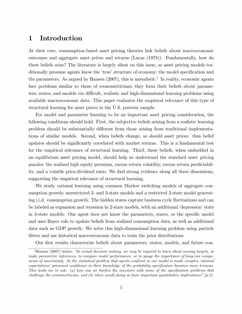
1 Introduction

At their core, consumption-based asset pricing theories link beliefs about macroeconomic

outcomes and aggregate asset prices and returns (Lucas (1978)). Fundamentally, how do

these beliefs arise? The literature is largely silent on this issue, as asset pricing models tra-

ditionally presume agents know the ‘true’structure of economy: the model specification and

the parameters. As argued by Hansen (2007), this is unrealistic.1 In reality, economic agents

face problems similar to those of econometricians: they form their beliefs about parame-

ters, states, and models via diffi cult, realistic and high-dimensional learning problems using

available macroeconomic data. This paper evaluates the empirical relevance of this type of

structural learning for asset prices in the U.S. postwar sample.

For model and parameter learning to be an important asset pricing consideration, the

following conditions should hold. First, the subjective beliefs arising from a realistic learning

problem should be substantially different from those arising from traditional implementa-

tions of similar models. Second, when beliefs change, so should asset prices: thus belief

updates should be significantly correlated with market returns. This is a fundamental test

for the empirical relevance of structural learning. Third, these beliefs, when embedded in

an equilibrium asset pricing model, should help us understand the standard asset pricing

puzzles: the realized high equity premium, excess return volatility, excess return predictabil-

ity, and a volatile price-dividend ratio. We find strong evidence along all three dimensions,

supporting the empirical relevance of structural learning.

We study rational learning using common Markov switching models of aggregate con-

sumption growth: unrestricted 2- and 3-state models and a restricted 2-state model generat-

ing i.i.d. consumption growth. The hidden states capture business cycle fluctuations and can

be labeled as expansion and recession in 2-state models, with an additional ‘depression’state

in 3-state models. Our agent does not know the parameters, states, or the specific model

and uses Bayes rule to update beliefs from realized consumption data, as well as additional

data such as GDP growth. We solve this high-dimensional learning problem using particle

filters and use historical macroeconomic data to train the prior distributions.

Our first results characterize beliefs about parameters, states, models, and future con-

1Hansen (2007) states: “In actual decision making, we may be required to learn about moving targets, tomake parametric inferences, to compare model performance, or to gauge the importance of long-run compo-nents of uncertainty. As the statistical problem that agents confront in our model is made complex, rationalexpectations’presumed confidence in their knowledge of the probability specification becomes more tenuous.This leads me to ask: (a) how can we burden the investors with some of the specification problems thatchallenge the econometrician, and (b) when would doing so have important quantitative implications" (p.2).

1

sumption dynamics (e.g., moments) over the postwar sample. Individual parameters and

model probabilities drift over time and, in particular, the agent perceives an upward drift

in the expected consumption growth, a strong secular decline in the consumption growth

volatility, and a decline in beliefs over large drops in consumption growth (such as the prob-

ability that consumption falls by more than 4% in a year). The agents learn about different

parameters at different speeds, and there is evidence for confounding effects.2 Non-stationary

beliefs should not be a surprise, they are a signature of parameter and model uncertainty

as beliefs are martingales, and shocks to beliefs are therefore permanent. This is easy to see

from the law of iterated expectations: e.g, for a parameter θ, E [θ|yt] = E [E [θ|yt+1] |yt] ,where yt denotes available data up until time t.

The beliefs generated by model and parameter learning are substantially different from

those generated from the models with fixed parameters estimated over the postwar sample. In

the fixed parameter models, the dynamics are driven solely by beliefs about the time-varying

Markov states and these shocks, by definition, are transient and do not drift over time.

Both experiments– model and parameter learning and a fixed parameter implementation–

capture business cycle fluctuations via state beliefs. Thus, the main difference is generated

by updates in parameter and model beliefs.

As mentioned earlier, if parameter and model learning are empirically important, updates

in beliefs about these dimensions of the consumption data should lead to changes in aggregate

asset prices. In support of this, we find strong evidence that quarterly excess stock market

returns are positively related to quarterly revisions in beliefs about expected consumption

growth. In these regressions, we control for contemporaneous realized consumption growth,

as well as updates in beliefs about expected consumption growth from the fixed parameter

models. Realized returns are also significantly and negatively related to shocks to predictive

consumption growth volatility. These results are strengthened if the agent learns from both

consumption and GDP growth. This is a particularly stringent test of a macro learning story

since changes in beliefs are driven completely by macroeconomic information.

Parameter and model learning are especially important for asset prices because they

generate long-run consumption risks (see Bansal and Yaron (2004)). Our approach allows

2There is significant learning about the expansion state parameters, slower learning about the recessionstate, and almost no learning about the disaster state, as it is rarely, if ever, visited. Standard large sampletheory implies that all parameters converge at the same rate, but the realized convergence rate, intuively,depends on the actual observed sample path. There is also strong evidence for a confounding effect: whenstates are unobserved, parameter learning is significantly slower, which implies that confounding leads tolonger-lasting learning effects.

2

us to identify and quantify these long-run risks from macro data alone, and we show that

with learning there is large time-variation in long-run beliefs. For example, defining long-run

shocks as changes in beliefs about expected discounted consumption growth from the current

time to infinity (as in shocks to the cash flow component of a Campbell-Shiller decomposi-

tion of the price-consumption ratio), we find that the volatility of long-run shocks from a

2-state model with parameter uncertainty is 3.4 times the volatility of the fixed parameters

counterpart over the postwar sample. Thus, these long-run risks are driven mainly by pa-

rameter and not state uncertainty. Long-run shocks are largest during recessions, as there

is more uncertainty about the parameters governing infrequent bad states, and therefore

more updating when these states are visited (see also Chen, Joslin, and Tran (2010)). This

contributes to the high volatility of returns in recessions.

To investigate the asset pricing implications of the estimated beliefs process, we consider

a formal equilibrium model assuming Epstein-Zin preferences. In particular, at each time t,

our agent prices a levered claim to future consumption given beliefs over parameters, models,

and states, computing quantities such as ex-ante expected returns and dividend-price ratios.

Then, at time t + 1, our agent updates beliefs using new macro realizations at time t + 1,

recomputes prices, expected returns and dividend-price ratios. From this time series of prices,

we compute realized equity returns, volatilities, etc. Thus, we feed in historically realized

macroeconomic data and analyze the asset pricing implications for this particular sample.

We use standard preference parameters taken from Bansal and Yaron (2004).

Solving the full pricing problem with priced parameter and model uncertainty is compu-

tationally prohibitive, as the dimensionality of the problem is too large. To price assets and

incorporate the time-varying parameter and model beliefs, we follow Piazzesi and Schneider

(2010) and Cogley and Sargent (2009) and use a version of Kreps’(1998) anticipated utility.

Anticipated utility implies that claims are priced at each point in time using current pos-

terior means for the parameters and model probabilities, assuming those values will persist

into the indefinite future. We do account for state uncertainty in this pricing exercise.

This pricing experiment provides additional evidence, along multiple dimensions, for the

importance of learning. The estimated fixed parameters 2- and 3-state models do not match

standard asset pricing moments: the realized equity premium, Sharpe ratio, the levels of

predictability, and price-dividend volatility are all much lower than those observed in the

data. Parameter and model learning uniformly improves all of these statistics, bringing

them close to observed values. Permanent revisions in beliefs, such as those generated by

parameter and model learning, have a particularly large impact on price-dividend ratios. The

3

substantial variation we document in parameter and model beliefs is therefore an important

source of excess return volatility. Moreover, price-dividend ratios generated by our learning

models have a significantly higher covariance with observed price-dividend ratios (15-30 times

higher) than those generated by the fixed parameter models. Overall, the agent perceives

the economy to have higher growth and be less risky than initially believed, and this also

generates ex post average excess returns about twice as large as the ex ante expected returns.

In terms of predictability, the returns generated by learning over time closely match the

data. In forecasting excess market returns with the lagged log dividend-price ratio, the

regression coeffi cients and R2’s are increasing with the forecasting horizon and similar to

those found in the data. The fixed parameters case, however, does not deliver significant

ex post predictability, although the ex ante risk premium is in fact time-varying in these

models as well, because the time-variation in the risk premium assuming fixed parameters is

too small relative to the volatility of realized returns to result in significant t-statistics. The

intuition for why in-sample predictability occurs when agents are uncertain about parameters

and models is the same as in Timmermann (1993) and Lewellen and Shanken (2002), and

can be understood as a strong form of the Stambaugh (1999) bias.

Our results are robust along a number of dimensions. We have considered several differ-

ent prior specifications. For instance, we present in an Online Appendix results from a case

where the prior parameter means are centered at the postwar maximum likelihood estimates.

Our findings are overall the same, both empirically and theoretically. Adding GDP growth

to investors information set only makes our main findings stronger. Finally, we solve the

fully rational pricing problem, where the representative agent prices the parameter uncer-

tainty ex ante, for a limited learning problem: the 2-state model where all the parameters

are unknown, but where the state is observed. This is a 9-dimensional problem and the most

complicated parameter learning problem it is computationally feasible to solve with reason-

able accuracy. The long-run risks induced by parameter learning are in this case priced risks,

which increases ex ante risk prices (see Collin-Dufresne, Johannes, and Lochstoer (2013)).

The main conclusions regarding the empirical relevance of structural learning are robust also

to this alternative pricing framework.

Below we relate our paper to the literature, Section 2 lays out the formal learning envi-

ronment, Section 3 characterizes the estimated time-series of beliefs, Section 4 shows results

from empirical tests that relate updates in beliefs to stock returns, while Section 5 present

the asset pricing implications of the estimated beliefs process.

4

1.1 Existing literature and alternative approaches for parameter,

state, and model uncertainty

Our paper is related to a large literature on learning and asset pricing (see Pastor and

Veronesi (2009) for a comprehensive review). Most of the literature studying the asset pric-

ing implications of parameter or state learning focuses on learning about a single unknown

parameter or state variable (assuming the other parameters and/or states are known) that

determines dividend dynamics and power utility. For example, Timmermann (1993) con-

siders the effect of uncertainty on the average level of dividend growth, assuming other

parameters are known, and shows in simple discounted cash-flow setting that parameter

learning generates excess volatility and patterns consistent with the predictability evidence

(see also Timmermann (1996)). Lewellen and Shanken (2002) study the impact of learning

about mean cash-flow parameters with exponential utility with a particular focus on return

predictability.

Veronesi (2000) considers the case of learning about mean-dividend growth rates in a

model with underlying dividend dynamics with power utility and focuses on the role of

signal precision or information quality. Pastor and Veronesi (2003, 2006) study uncertainty

about a fixed dividend-growth rate or profitability levels with an exogenously specified pricing

kernel, in part motivated in order to derive cross-sectional implications. Weitzman (2007)

and Bakshi and Skoulakis (2009) consider uncertainty over volatility.

Cogley and Sargent (2008) consider a 2-state Markov-switching model, parameter un-

certainty over one of the transition probabilities, tilt beliefs to generate robustness via pes-

simistic beliefs, and use power utility. After calibrating the priors to the 1930s experience,

they simulate data from a true model calibrated to the post War experience to show how

priced parameter uncertainty and concerns for robustness impact asset prices, in terms of

the finite sample distribution over various moments. Cogley and Sargent (2009) consider the

differences between anticipated utility and full learning in simple macroeconomics models

and find small differences. Due to its computational advantages, anticipated utility is the

dominant approach in macroeconomics for handling parameter learning.

A number of papers consider state uncertainty, where the state evolves discretely via a

Markov switching model or smoothing via a Gaussian process. Moore and Shaller (1996) con-

sider consumption/dividend based Markov switching models with state learning and power

utility. Brennan and Xia (2001) consider the problem of learning about dividend growth

which is not a fixed parameter but a mean-reverting stochastic process, with power utility.

5

Veronesi (2004) studies the implications of learning about a peso state in a Markov switching

model with power utility. David and Veronesi (2010) consider a Markov switching model

with learning about states.

In the case of Epstein-Zin utility, Brandt, Zeng, and Zhang (2004) consider alternative

rules for learning about an unknown Markov state, assuming all parameters and the model

is known. Lettau, Ludvigson, and Wachter (2008) consider information structures where

the economic agents observe the parameters but learn about states in Markov switching

consumption based asset pricing model. Chen and Pakos (2008) consider learning about the

mean of consumption growth which is a Markov switching process. Ai (2010) studies learning

in a production-based long-run risks model with Kalman learning about a persistent latent

state variable. Bansal and Shaliastovich (2008) and Shaliastovich (2010) consider learning

about the persistent component in a Bansal and Yaron (2004) style model with sub-optimal

Kalman learning.

2 The Environment

2.1 Model

Consider a Markov switching model for aggregate, real, per capita consumption growth:

∆ct = µst + σstεt, (1)

where ∆ct is log-consumption growth, εti.i.d.∼ N (0, 1), st ∈ {1, ..., N} is a discrete-time

Markov chain with transition matrix Π, and(µst , σ

2st

)are the state-dependent mean and

variance. The transition probabilities are defined as P [st = j|st−1 = i] = πij with∑N

j=1 πij =

1. We consider general 2- and 3-state models and an i.i.d. 2-state model that assumes

π11 = π21 and π22 = π12 = 1 − π11, generating an i.i.d. mixture of normal distributions.

The unrestricted 2- and 3-state models have 6 and 12 static parameters, respectively and

the i.i.d. two state model has 5 static parameters.

Since Mehra and Prescott (1985) and Rietz (1988), Markov switching models are com-

monly used for modeling aggregate consumption dynamics due to their flexibility and tractabil-

ity. Recently, Barro (2006, 2009), Barro and Ursua (2008), Barro, Nakamura, Steinsson and

Ursua (2009), Backus, Chernov, and Martin (2009), and Gabaix (2009) use these models

to study consumption disasters. The models generate a range of economically interesting

6

and statistically flexible distributions by varying the number, persistence, and distribution

of states, even though the εt’s are i.i.d. normal. Markov switching models are also tractable,

as likelihood functions and filtering distributions are analytic, conditional on parameters. It

is common to provide business cycle labels to the states, and to preview some of our results,

we estimate states, in the unrestricted 2-state model, that correspond closely to recessions

and expansions, while the 3-state model also has a rare ‘Depression’state.

2.2 Information and learning

To operationalize the model, we need to specify how and from what our agent learns over

time. As our main goal is to study an agent facing the same inference problems as an econo-

metrician, we assume the agent does not know the Markov state, the true parameters, or the

true specification. We refer to these unknowns as state, parameter, and model uncertainty.

Our agent learns rationally from current and past consumption growth, updating beliefs

using Bayes rule as new data arrives. The primary data is the ‘standard’data set used in

the consumption-based asset pricing literature– final real, per capita quarterly growth in

services and nondurable consumption as given in the National Income and Product Account

tables from the Bureau of Economic Analysis from 1947:Q1 until 2009:Q1. Although we

consider consumption-based asset pricing models, agents could learn from other macroeco-

nomic data about consumption dynamics. We develop an extension to handle this problem

and implement a case of learning using consumption and GDP growth data.

Formally, the learning problem is as follows. Mk indexes a model, k = 1, ..., K, and a

given model has states, st, and parameters, θ.3 The posterior distribution, p (θ, st,Mk|yt) ,summarizes beliefs after observing data yt = (y1, ...yt) and is given by

p(θ, st,Mk|yt

)= p

(θ, st|Mk, y

t)P(Mk|yt

). (2)

p (θ, st|Mk, yt) solves the parameter and state “estimation”problem conditional on a model

and P (Mk|yt) provides model probabilities and solves the model learning problem. Thelearning process refers to how the posterior distribution sequentially changes over time, as the

agents beliefs evolve as a function of the specific observed sequence of macroeconomic data

during the postwar sample. This learning problem is a diffi cult high-dimensional problem, as

3This is a notational abuse. In general, the state and dimension of the parameter vector should depend onthe model, thus we should superscript the parameters and states by ‘k’, θk and skt . For notational simplicity,we drop the model dependence and denote the parameters and states as θ and st, respectively.

7

posterior beliefs depend in a complicated, non-analytical manner on past data and can vary

substantially over time. A description of our econometric approach for posterior sampling

(particle filtering) is in the Online Appendix.

In general, posterior beliefs over fixed quantities like parameters and model indicators

are martingales. This has the crucial implication that shocks to beliefs over θ andMk af-

fects the agent’s expectations of consumption growth indefinitely into the future, generating

truly long-run risks. These permanents effects are the signature or hallmark of parame-

ter/model learning and can be contrasted with the transient nature of beliefs over st, which

mean-revert over time. Bansal and Yaron (2004) show that long-run risks have important

asset pricing implications, but empirically identifying these long-run risks is diffi cult. Our

empirical strategy identifies and quantifies one source of these long-run risks, the perma-

nent updates arising from rational parameter and model learning (see also Collin-Dufresne,

Johannes, and Lochstoer (2013)).

Our analysis differs from existing work on learning in an asset pricing setting (see Pastor

and Veronesi (2009) for a recent survey) along three key dimensions. First, we consider simul-

taneous learning about parameters, hidden state variables, and even model specifications–

i.e., the learning problem closely mimics that of the real-world econometrician. Most exist-

ing work focuses on learning a single parameter or state variable. Learning about multiple

unknowns is more diffi cult as additional unknowns often confounds inference, slowing the

learning process. Second, we focus on the specific implications of sequential learning about

aggregate consumption dynamics from macroeconomic data during the U.S. post World War

II experience. Thus, we are not expressly interested in general asset pricing implications

of learning in repeated sampling settings, but rather the specific implications generated by

the historical macroeconomic shocks realized in the United States over the last 65 years.

Third, we use a new and stringent test of learning that relates updates in investor beliefs

about aggregate consumption dynamics to realized equity returns. If learning is important

for asset price dynamics, the historical time-series of beliefs should be strongly related to the

historical time-series of aggregate asset prices.

2.3 Initial beliefs

The learning process begins with initial beliefs– the prior distribution. In terms of func-

tional forms, we assume proper, conjugate prior distributions (Raiffa and Schlaifer (1956)).

Conjugate priors imply that the functional form of beliefs is the same before and after sam-

8

pling (beliefs are closed under sampling); they are analytically tractable for econometric

implementation; and they are flexible enough to express a wide range initial beliefs.

The conjugate prior for location/scale parameters is

p(µi, σ2i ) = p(µi|σ2

i )p(σ2i ) ∼ NIG(ai, Ai, bi, Bi),

where NIG is the normal/inverse gamma distribution, generating a fat-tailed t-distributedmarginal prior for µi, adding a layer of robustness. The Beta/Dirichlet distribution is a

conjugate prior for transition probabilities. Conjugate priors are commonly used since flat

or ‘uninformative’priors can not be used with Markov switching models, as they generate

identification issues (the label switching problem) and improper posterior distributions.4

We endow our agent with economically motivated and realistic initial beliefs, using a

training sample to specify the prior parameters. Training samples use an initial data set to

inform the parameter location and scale and are a common way of generating data-based

reference priors. We use Shiller’s annual consumption data from 1889 until 1946. The use

of prewar macroeconomic data as a prior training sample does create some issues. Most

notably, there is evidence for a structural break in the quality of macroeconomic data (see

Romer (1989)) and the parameters need to be converted from annual to quarterly data,

which is only available starting in 1947. Romer (1989) presents evidence that a substantial

fraction of the volatility of macro variables such as consumption growth pre-WW2 is due to

measurement error. To account for this, we set the prior mean over the volatility parameters

in 1947Q1 to a quarter of the value estimated over the annual Shiller sample. To add an

additional layer of robustness, we use a 10-year burn-in period of quarterly data in the

postwar sample, updating beliefs using the quarterly NIPA data from 1947 through 1956.

Thus, our pricing exercises begins in 1957Q1, proceeding through 2009Q1. Further prior

details are in the Online Appendix.5

4The label switching problem refers to the fact that the likelihood function is invariant to a relabeling of thecomponents, thus the parameters are not uniquely identified. For example, in a 2-state model, it is possibleto swap the definitions of the first and second states and the associated parameters without changing thevalue of the likelihood. Identification, for either Bayesian or classical methods, requires additional constraintssuch as ordering of the means or variances of the parameters. For discussions of these issues, see Marin,Mengersen, and Robert (2005) or Fruhwirth-Schnatter (2006).

5For robustness, we also considered alternative priors. Earlier drafts used priors centered at the estimatedvalues from the Shiller sample, but with substantially larger prior variances to capture the idea that anagent in 1947 would not have taken the pre-war sample at face value and would have allowed for moreuncertainty. We also considered a rational expectations or ‘look-ahead’prior centered at postwar full-sampleparameter estimates (see Online Appendix). In both cases, all of our main results hold, both qualitativelyand quantitatively.

9

We contrast our learning results with those from a model with ‘fixed parameter’priors.

This is a point-mass prior located at the parameter MLE for a given model estimated on the

postwar period. In this case, the agent only learns about the latent Markov state, which is

the typical rational expectations approach which assumes the agent knows the most likely

parameters. Contrasting the full-learning and fixed-parameter cases allows us to separately

identify the roles of state and parameter learning.

Table 1 - Priors (1957Q1) and end-of-sample posteriors (2009Q1)

Table 1: The table shows the 1957Q1 priors for the parameters of the three different models oflog, real per capita, quarterly consumption gorwth considered in the paper, as well as the end-of-sample posteriors (as of 2009Q1). The parameters within a state (mean and variance) haveNormal/Inverse Gamma distributed priors, while the transition probabilities have Beta distributedpriors. Note that π̂ij ≡ πij

1−πij .

Panel A: Priors and end-of-sample posteriors for i.i.d. model

Parameter µ1 µ2 σ21 σ2

2 π11

Prior mean 0.60% -1.56% 0.59 (%)2 2.78 (%)2 5.51%

Prior st.dev. 0.11% 0.73% 0.14 (%)2 1.31 (%)2 3.80%

Posterior mean 0.61% -0.96% 0.25 (%)2 2.39 (%)2 3.79%Posterior st.devPrior st.dev 31% 73% 21% 73% 49%

Panel B: Priors and end-of-sample posteriors for 2−state model

Parameter µ1 µ2 σ21 σ2

2 π11 π22

Prior mean 0.81% -0.03% 0.40 (%)2 0.84 (%)2 0.88 0.83

Prior st.dev. 0.18% 0.28% 0.16 (%)2 0.23 (%)2 0.07 0.09

Posterior mean 0.70% 0.13% 0.15 (%)2 0.63 (%)2 0.93 0.83Posterior st.devPrior st.dev 18% 41% 11% 51% 34% 70%

Panel C: Priors and end-of-sample posteriors for 3−state model

Parameter µ1 µ2 µ3 σ21 σ2

2 σ23 π11 π̂12 π̂21 π22 π̂31 π33

Prior mean 0.74% -0.23% -1.84% 0.52 (%)2 0.55 (%)2 0.56 (%)2 0.92 0.86 0.86 0.75 0.35 0.65

Prior st.dev. 0.17% 0.29% 0.47% 0.15 (%)2 0.21 (%)2 0.28 (%)2 0.05 0.13 0.01 0.08 0.24 0.10

Posterior mean 0.72% 0.01% -1.77% 0.18 (%)2 0.45 (%)2 0.56 (%)2 0.94 0.93 0.92 0.77 0.34 0.65Posterior st.devPrior st.dev 22% 42% 98% 14% 46% 95% 40% 54% 60% 85% 97% 99%

10

To summarize parameter prior beliefs, Table 1 reports the prior means and dispersion.

The unrestricted 2-state model priors correspond to business cycle fluctuations, with slightly

negative consumption growth in recessions that are persistent but shorter-lived than the high

growth expansions. The 3-state model has an additional rare and short-lived ‘Depression’

state, with a mean expected quarterly growth rate of −1.8%. This is low and reasonable,

but certainty not a consumption disaster. The low growth state in the i.i.d. 2-state model is

in between the recession and the depression states of the 3-state model. The prior standard

deviation of the mean in the good state in the 3-state model is 0.17%, whereas the prior

standard deviation of the mean in the Depression state is 0.47%, reflecting the fact that

historically there are more observations drawn from the good state than from the recession

state than from the depression state. In sum, the information in the training sample leads

to priors that embody reasonable properties given the pre-WWII data, as well as the 1947

to 1956 burn-in period, used to train the priors.

To incorporate model uncertainty, we need to specify initial probabilities of the three

models at the beginning of the postwar sample. There is good reason to consider all of these

models ex-ante possible. The i.i.d. consumption growth model is a benchmark model in the

literature, as a natural outcome of the permanent income hypothesis (see Friedman (1957),

Hall (1978), Campbell and Cochrane (1999)). On the other hand, business cycle fluctuations

are well-documented, supporting a persistent 2-state model (Kandel and Stambaugh (1990)).

Similarly, the Great Depression which was fresh in investors minds in 1947, would suggest

the importance of a third ‘crisis’ state. In fact, there has been a resurgence of interest

models with ‘disaster’states in the macro-finance literature (see, e.g., Rietz (1988), Barro

(2006, 2009)). For simplicity, we specify equal model probabilities for each model in 1947

and use the 10-year burn-in period from 1947 to 1956 to update these model priors. One of

our main results is that the 2-state model provides a dramatically better fit to the postwar

data, which implies that our results are not sensitive to reasonable variation in this prior

assumption. In addition to model averaged results, we separately report results for the each

of the individual models in the following.

3 Characterizing the time series of beliefs

This section summarizes the agent’s dynamic learning process over the post-WW2 sample,

including the initial burn-in period from 1947 to 1956. We discuss state, parameter, and

model learning, then implications for the time series of conditional consumption moments,

11

as well as long-run consumption growth dynamics.

3.1 State, parameter, and model learning

For a given model, the agent learns about parameters and states, with belief updates driven

by a combination of the specific sequence of realized data, model specification, and initial

beliefs. To start, consider state beliefs, where state 1 is an ‘expansion’state, state 2 the

‘recession’state and, if a 3-state model, state 3 the ‘Depression’state. Figure 1 reports state

estimates, E [st|Mk, yt]. Note that this quantity is marginal, integrating out parameter

uncertainty. Although st is discrete, the mean estimates are not integer valued.

First, state beliefs primarily capture business cycle fluctuations, as they are strongly

related to NBER recessions (shaded yellow) and expansions, especially in the unrestricted 2-

and 3-state models. The only exceptions are the mild recessions in the late 1960s and 2001,

which did not have substantial consumption declines. This implies that state beliefs largely

capture the transitory and stationary aspects of business cycle fluctuations. Second, there is

a strong difference across models in state persistence. The i.i.d. model identifies recessions

as one-off transient negative shocks, while the 2- and 3-state models identify persistent

recession states. Only two periods place even modest probability on the Depression state

— the recession in 1980 and the financial crisis in 2008. Depression states are essentially

‘Peso’events in the postwar sample, something that would have been diffi cult to forecast in

1947. Third, state beliefs are more volatile early in the sample in all models, due to higher

parameter uncertainty, which, in turn, makes state identification more diffi cult.

Next, consider the dynamics of parameter beliefs. For parsimony, we focus on a few

economically interesting and important parameters in the 2-state model as the next section

provides additional details for all of the models. The top panels of Figure 2 document a

gradual decline in the posterior means of σ21 and σ

22 over the postwar sample, a combination

of the Great Moderation (realized consumption volatility decreased over time) and initial

beliefs, which are based on a historical experience with higher consumption growth volatility.

The decline in consumption volatility in the expansion state is quite large, from about 0.7%

per quarter to about 0.4% per quarter.

The lower panels in Figure 2 display the mean beliefs over the transition probabilities,

π11 and π22. After the 10-year burn-in period, the former essentially increases over the

sample, while the latter decreases. That is, 50 years of, on average, long expansions and

high consumption growth generates revisions in beliefs consistent with more persistent good

12

Figure 1 - Evolution of Mean State Beliefs

1947 1956 1965 1974 1983 1992 2001 20101

1.2

1.4

1.6

1.8

2Mean State Beliefs in i.i.d. Model

Years

1947 1956 1965 1974 1983 1992 2001 20101

1.2

1.4

1.6

1.8

2Mean State Beliefs in 2­State Model

Years

1947 1956 1965 1974 1983 1992 2001 20101

1.5

2

2.5Mean State Beliefs in 3­State Model

Years

Figure 1: The plots show the means of agents’beliefs about the state of the economy at each pointin time, Et[st]. Note that st = 1, 2 in the i.i.d. and the 2-state model, while st = 1, 2, 3 in the3-state model. ’1’is an expansion state, ’2’is a recession state, and ’3’is a disaster state. Thus,the mean state belief is between 1 and 2 for the 2-state models, and between 1 and 3 for the 3-statemodel. The time t state beliefs are formed using the history of consumption only up until andincluding time t. The "i.i.d. Model" is a model with i.i.d. consumption growth but that allows forjumps (’2’is a jump state). The sample is from 1947:Q2 until 2009:Q1.

13

states and less persistent bad states. The conditional probability of staying in an expansion,

increases from 0.88 to 0.93. Thus, there is non-stationary drifts in parameter beliefs–

permanent shocks– that generate changes in beliefs over long-run consumption dynamics.

These drifts can have first order asset pricing implications. For both variances and transition

probabilities, the specific sequence of realized data generated positive shocks to the agents’

beliefs that, all else equal, will lead to higher ex post equity returns relative to ex ante

expectations. Later, we quantify these effects.

Figure 3 displays model probabilities over time.6 Note first that the probability of the

i.i.d. model increases until the early 1960s and then rapidly decreases in the late 1960s and

1970s, due to the persistently high growth, low volatility expansion in the 1960s and the

persistently low growth and high volatility recessions in the 1970s. Thus, it does not take

long for a Bayesian agent to learn consumption growth is not i.i.d. This conclusion is robust

even if the prior probability of the i.i.d. model is set to 0.95 - in this case it takes somewhat

longer (but still only slightly more than half the sample) for the probability of the i.i.d.

model to become negligible.7

The 2-state model dominates, as the 3-state model has less than a 1% probability and the

i.i.d. model is effectively zero at the end of the sample. The 2-state model fits the postwar

sample so well precisely because there were no severe consumption recessions. This result

does not mean an investor should not have considered the 3-state model in 1947 or should

not consider the 3-state model going forward. After World War II, it was natural for an

agent to allow for the possibility of a model with severe recessions and, moreover, it would

seem odd if an agent did not allow for this given the extreme level of macroeconomic and

political uncertainty present in 1947. Looking forward, even though the 3-state model has

a low posterior probability, a single severe consumption recession would drastically increase

the probability of the 3-state model, as these shocks are highly unlikely in the 2-state model.

In particular, four consecutive quarters if -2% growth, makes the model probability of the

3-state model jump from 0.2% to 68.4%. Such a large consumption drop was exactly the

6Note that marginal model probabilities (i.e., where parameter uncertainty is integrated out) penalizesextra parameters as more sources of parameter uncertainty tends to flatten the likelihood function. Thus,it is not the case, as we see an example of here, that a 3-state model always dominates a 2-state model inBayesian model selection.

7This result holds for various prior specifications and is robust to time-aggregation. In the Online Appen-dix, we show that taking out an autocorrelation of 0.25 from the consumption growth data, which is whattime-aggregation of i.i.d. data predicts (see Working (1960)), does not qualitatively change these results - ifanything it makes the rejection of the i.i.d. model occur sooner. The same is true if we purge the data of itsfull sample first order autocorrelation.

14

Figure 2 - Evolution of Mean Parameter Beliefs

1947 1956 1965 1974 1983 1992 2001 20100.1

0.2

0.3

0.4

0.5

0.6

Posterior Means of σ12 in 2­state Model

Years1947 1956 1965 1974 1983 1992 2001 2010

0.7

0.8

0.9

1

1.1

Posterior Means of σ22 in 2­state Model

Years

1947 1956 1965 1974 1983 1992 2001 20100.86

0.88

0.9

0.92

0.94

0.96

Posterior Means of π11 in 2­state Model

Years1947 1956 1965 1974 1983 1992 2001 2010

0.8

0.82

0.84

0.86

0.88

0.9

Posterior Means of π22 in 2­state Model

Years

Figure 2: The two top plots in this figure show the mean beliefs about the variance parameterswithin each state for the 2-state model (σ2

1 is the variance parameter in the ’expansion’state, whileσ2

2 is the variance parameter in the ’recession’state). The two lower plots show for the same modelthe mean beliefs of the probabilities of remaining in the current state (π11 is the probability ofstaying in the ’expansion’state, while π22 is the probability of staying in the ’recession’state). Thesample is from 1947:Q2 until 2009:Q1.

15

outcome in 1932 (-8%). These sorts of shocks are certainly not out of the question, especially

after the financial crisis where there was a widespread discussion of the possibility of another

Great Depression.

Additionally, these results are likely conservative in terms of the model probabilities for

the 3-state model. The likelihood of the 3-state model increases when additional macroeco-

nomic variables are included or under less restrictive prior distributions. The 3-state model,

even though its probability falls throughout much of the sample, also provides important

pricing benefits, as discussed later.

3.1.1 Speed of learning and confounding effects

Table 1 reports end-of-sample (2009Q1) posterior means and standard deviations for each

parameter, where the latter is expressed as a fraction of the 1957Q1 standard deviation of

beliefs. This quantifies the total ‘amount’of learning over the sample.

As noted earlier, the agent updates mean beliefs in the overall direction of a less-risky

world– expansions last longer, recessions are less severe, and volatilities are lower at the end

of the sample. Importantly, the speed of learning varies significantly across parameters. In

general, there is more learning about expansions than recessions, and, in turn, more learning

about recessions than a Depression. For example, in the 3-state model, the posterior standard

deviations for the good state parameters, µ1 and σ21 decrease 78% and 86%. The decrease

for the recession state parameters is less: µ2 and σ22 decrease by 58% and 54%, respectively.

At the same time, the posterior uncertainty over µ3, σ23, π33, and π31 barely decreases at all.

This indicates there is very little learning about the Depression state in the 3-state model.

Empirically, documenting that the speed of learning varies dramatically across parame-

ters is intuitive– some parameters are harder to learn than others– and lends support to

arguments that a high level of parameter uncertainty is a likely feature of models with a

rarely observed state and is an important feature for disaster risk models (see Chen, Joslin,

and Tran, 2010). This also implies that there will be a large ‘amount’of learning when and

if the disaster state is reached.

Learning about multiple unknowns can introduce confounding effects– e.g., the fact that

it is more diffi cult to learn in settings when multiple parameters and/or states are uncertain

than in a setting where a single parameter or just the states are unknown. We find that the

principal confounding effect is joint learning about the unobserved state and parameters. To

quantify the confounding effects of state and parameter learning, Table 2 shows the results

16

Figure 3 - Marginal Model Probabilities

1950 1960 1970 1980 1990 20000

0.2

0.4

0.6

0.8

1Sequential model probabili ties with equal model prior

1950 1960 1970 1980 1990 20000

0.2

0.4

0.6

0.8

1Sequential model probabili ties with equal model prior, exc luding the i.i .d. model

i.i .d.2­State3­State

2­State3­State

Figure 3: The top panel shows the evolution of the probability of each model being the true model,where the models at the beginning of the sample are set to have an equal probability, and wherestate and parameter uncertainty have been integrated out. The model probabilities sum to 1 at alltimes, and each model’s probability is then represented by the area the model’s color (dark bluefor i.i.d., bright red for 2-state and bright green for 3-state) occupies in the graph at each point intime. The lower plot shows the same when the agent considers only the general 2-state and 3-statemodels as possible models of consumption dynamics, again with equal initial model probabilities.The sample period is 1947:Q2 - 2009:Q1.

17

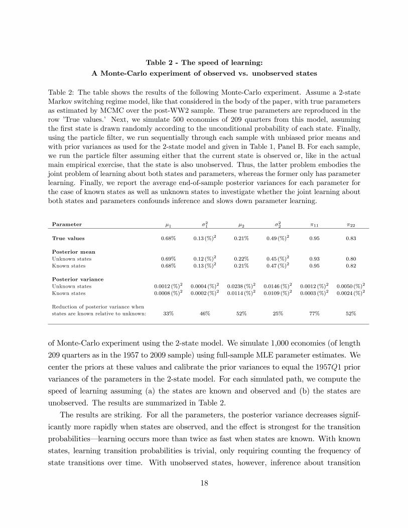
Table 2 - The speed of learning:A Monte-Carlo experiment of observed vs. unobserved states

Table 2: The table shows the results of the following Monte-Carlo experiment. Assume a 2-stateMarkov switching regime model, like that considered in the body of the paper, with true parametersas estimated by MCMC over the post-WW2 sample. These true parameters are reproduced in therow ’True values.’ Next, we simulate 500 economies of 209 quarters from this model, assumingthe first state is drawn randomly according to the unconditional probability of each state. Finally,using the particle filter, we run sequentially through each sample with unbiased prior means andwith prior variances as used for the 2-state model and given in Table 1, Panel B. For each sample,we run the particle filter assuming either that the current state is observed or, like in the actualmain empirical exercise, that the state is also unobserved. Thus, the latter problem embodies thejoint problem of learning about both states and parameters, whereas the former only has parameterlearning. Finally, we report the average end-of-sample posterior variances for each parameter forthe case of known states as well as unknown states to investigate whether the joint learning aboutboth states and parameters confounds inference and slows down parameter learning.

Parameter µ1 σ21 µ2 σ2

2 π11 π22

True values 0.68% 0.13 (%)2 0.21% 0.49 (%)2 0.95 0.83

Posterior meanUnknown states 0.69% 0.12 (%)2 0.22% 0.45 (%)2 0.93 0.80

Known states 0.68% 0.13 (%)2 0.21% 0.47 (%)2 0.95 0.82

Posterior varianceUnknown states 0.0012 (%)2 0.0004 (%)2 0.0238 (%)2 0.0146 (%)2 0.0012 (%)2 0.0050 (%)2

Known states 0.0008 (%)2 0.0002 (%)2 0.0114 (%)2 0.0109 (%)2 0.0003 (%)2 0.0024 (%)2

Reduction of posterior variance whenstates are known relative to unknown: 33% 46% 52% 25% 77% 52%

of Monte-Carlo experiment using the 2-state model. We simulate 1,000 economies (of length

209 quarters as in the 1957 to 2009 sample) using full-sample MLE parameter estimates. We

center the priors at these values and calibrate the prior variances to equal the 1957Q1 prior

variances of the parameters in the 2-state model. For each simulated path, we compute the

speed of learning assuming (a) the states are known and observed and (b) the states are

unobserved. The results are summarized in Table 2.

The results are striking. For all the parameters, the posterior variance decreases signif-

icantly more rapidly when states are observed, and the effect is strongest for the transition

probabilities– learning occurs more than twice as fast when states are known. With known

states, learning transition probabilities is trivial, only requiring counting the frequency of

state transitions over time. With unobserved states, however, inference about transition

18

probabilities depends on inference on the specific state transitions taken over the sample,

which in turn, depend on parameter beliefs at each point in time, which also depend on the

specific path of observed data.

Overall, the results show that learning speeds vary substantially across parameters and

there are strong confounding effects in realistic learning settings. Because prior research

largely focusses on learning about a single parameter or state variable and often in theoretical

settings, these effects have not been documented previously. Both of these effects have

important asset pricing implications, which are discussed in Section 5.

3.2 Beliefs about conditional consumption growth moments

In consumption-based asset pricing models, the conditional dynamics of consumption growth–

and not the variation in individual parameters, states or models– drives the asset pricing

implications. As an example, consider the conditional volatility of consumption growth. A

decrease in the probability of the bad state, which has higher consumption growth volatility,

could be offset by an increase in the consumption volatility in the good state, σ1, keeping

the total conditional volatility of consumption growth constant. To summarize learning in

an asset pricing relevant manner, we therefore report the agent’s beliefs about key short-

and long-run moments of consumption growth.

3.2.1 Short-run moments

Figures 4 and 5 show the conditional quarterly mean and standard deviation of consumption

growth over the postwar sample for each model (assuming parameter and state learning),

the full learning model including model averaging, as well as for the fixed parameter 3-state

model. All of these quantities are marginal, integrating out parameter, state, and/or model

uncertainty. Focusing first on the fixed parameters case, the conditional mean and variance

fluctuations are strongly business cycle related. This is to be expected as states are directly

linked to business cycles. Expected quarterly consumption growth is about 0.3% in recessions

and 0.6% in expansions, while volatility is about 0.9% in recessions and 0.45% in expansions.

Notably, there is no strong drift in either moment over the sample– again, this is natural

given the cyclical nature of the states and since there are many business cycles in the sample.

The learning models, with the exception of the i.i.d. model, show similar business cycle

fluctuations in both the mean and the volatility. In particular, for both the 2- and 3-state

models the expected consumption growth is again about 0.3% in recessions and about 0.6% in

19

Figure 4 - Quarterly Mean of Consumption Growth

1947 1956 1965 1974 1983 1992 2001 2010­0.4

­0.2

0

0.2

0.4

0.6

0.8

1

Years

Per

cent

age 

(per

 qua

rter)

Expected quarterly consumption growth from learning models

Full modeli.i.d.2­State3­State

1947 1956 1965 1974 1983 1992 2001 2010­0.4

­0.2

0

0.2

0.4

0.6

0.8

1

Years

Per

cent

age 

(per

 qua

rter)

Expected quarterly consumption growth: full learning model vs fixed parameters case

Full learning model3­State fixed parameters

Figure 4: The top panel shows the quarterly conditional expected consumption growth, where stateand parameter uncertainty have been integrated out, from each of the three benchmark models:the "i.i.d.", and the general 2- and 3-state switching regime models. The solid line shows theconditional expected consumption growth rate for the ’full’model, where also model uncertaintyhas been integrated out. The lower plot shows again the conditional expected consumption growthfor the full learning model (solid line), but adds the same moment from the fixed parameter 3-statemodel (dotted line). The sample period is 1947:Q2 - 2009:Q1.

20

expansions, which implies that model uncertainty is not central for this particular moment.

There is an overall increase in expected quarterly consumption growth over the sample,

consistent with the updates in transition probabilities associated with the surprisingly long

expansions and short and mild recessions (see Figure 2).

The conditional volatility of quarterly consumption growth is about twice as high in

recessions as in expansions also in the learning models. However, there is a strong downward

drift in the conditional volatility in all the learning models. The predictive conditional

volatility of consumption growth in expansions decreases from more than 1% per quarter to

about 0.5% at the end of the sample. This reflects in part the Great Moderation– the fact

that realized consumption volatility decreased over the postwar sample, which in turn leads

to downward revisions in the volatility parameters– and also a general decrease in parameter

uncertainty as the agent learns over time.

In terms of the conditional volatility, model learning increases the downward drift, exac-

erbating the Great moderation. The 3-state model has a higher overall conditional consump-

tion volatility than the 2-state model due to the presence of the Depression state. At the

same time, the probability of the 3-state model is decreasing over the sample, which shows

how model uncertainty, like parameter uncertainty, contributes to non-stationary changes in

beliefs.

3.2.2 Long-run moments

Bansal and Yaron (2004) highlight the first order importance of long-run consumption risks

for asset pricing when agents have a preference for an early resolution of uncertainty. Para-

meter and model learning creates a natural source of truly long run consumption risks, as

changes in beliefs persist indefinitely into the future, affecting the distribution of consump-

tion growth forever. Our empirical approach allows us to quantify these long-run shocks in

the postwar sample.

To do this, we compute shocks to long-run expected consumption growth, which we define

as Et[∑∞

j=1 ρj∆ct+j

], where ρ is set to 0.99 and the expectation integrates out state and

parameter uncertainty.8 To focus the issues, we consider the 2-state model, as the results

are similar for other models and model averaged long-run consumption growth.

8The discount parameter, ρ, is important for the definition of the long-run shocks. In particular, with thepermanent shocks induced by parameter learning, the long-run shock would be infinite with ρ = 1, whereasthe transient shocks in the model with stationary state learning would be finite. Our chosen value of ρ = 0.99corresponds to an annual discount of 0.96 which is not particularly high and, if anything, conservative.

21

Figure 5 - Quarterly Standard Deviation of Consumption Growth

1947 1956 1965 1974 1983 1992 2001 20100.4

0.5

0.6

0.7

0.8

0.9

1

1.1

1.2

1.3

Years

In p

erce

nt (p

er q

uarte

r)Conditional standard deviation of quarterly consumption growth from learning models

Full modeli.i.d.2­State3­State

1947 1956 1965 1974 1983 1992 2001 20100.4

0.5

0.6

0.7

0.8

0.9

1

1.1

1.2

1.3

Years

In p

erce

nt (p

er q

uarte

r)

Conditional standard deviation of quarterly consumption growth: full learning model vs. fixed parameters

Full learning model3­state fixed parameters

Figure 5: The top panel shows the quarterly conditional standard deviation of consumption growth,where state and parameter uncertainty have been integrated out, from each of the three benchmarkmodels: the "i.i.d.", and the general 2- and 3-state switching regime models. The solid line shows theconditional standard deviation for the ’full’model, where also model uncertainty has been integratedout. The lower plot shows again the quarterly conditional standard deviation of consumption growthfor the full learning model (solid line), but adds the same moment from the fixed parameter 3-statemodel (dotted line). The sample period is 1947:Q2 - 2009:Q1.

22

The top plot in Figure 6 displays long-run expected consumption growth shocks in the

2-state models with either parameter uncertainty or fixed known parameters. There are a

number of important results. First, these long-run shocks are much more volatile– in fact,

3.4 times more volatile– with unknown parameters. Thus, parameter learning generates

quantitatively large long-run consumption growth shocks, and the learning setup we propose

here provides a way to identify these shocks sequentially in the data. These permanent shocks

to long-run beliefs have a large impact on aggregate valuation ratios and thus help generate

substantial excess return volatility. Further, to the extent the preference specification prices

such long-run risk, parameter uncertainty can be a significant additional source of macro

risk (see Collin-Dufresne, Johannes, and Lochstoer (2013)).

Second, the largest shocks to long-run consumption growth occur during recessions, be-

cause there is more uncertainty over recession/Depression state parameters and consumption

observations are more volatile in these periods. Thus, parameter learning generates counter-

cyclical volatility of long-run risks. Further, this crucially provides an explanation for why

equity returns are so volatile in recessions: not only do state transitions generate high volatil-

ity, but parameter updating generates quantitative large, permanent shocks to beliefs during

recessions.

The lower plot of Figure 6 compares the shocks to long-run expected consumption growth

from a 2-state model to those from a simple i.i.d. lognormal model, in both cases with

unknown parameters. This 1-state model features no state uncertainty, captures uncertainty

about the two first moments of consumption growth in the simplest possible fashion, and is

calibrated to, in 1889, have the same prior beliefs about the mean and variance parameters

as for the good state of the 2-state model (see the Online Appendix for details on these

priors). Thus, the difference in the long-run shocks from these models measures the added

long-run consumption risks arising from a realistic, high-dimensional learning problem. The

volatility of long-run consumption shocks is much higher (2.8 times) in the general 2-state

model than in the 1-state i.i.d. model. Thus, parameter learning in a simple 1-state setting

generates volatility of long-run shocks just slightly higher than those from the 2-state model

with fixed parameters and unobserved states.

The two plots in Figure 6 show how parameter learning is an important source of long-

run risk shocks, highlighting the importance of realistic learning problems and confound-

ing effects. The magnitude of these long-run risk shocks is particularly large in economic

downturns, as the agent is more uncertain about parameters governing such less frequently

observed states.

23

Figure 6 - Long-run consumption shocks

1960 1970 1980 1990 2000­4

­3

­2

­1

0

1

2

3

Year

Long

­run

 con

sum

ptio

n sh

ocks

Long­run shocks to consumption in 2­state model with and without parameter uncertainty

Unknown parametersFixed parameters

1958 1968 1978 1988 1998 2008­4

­3

­2

­1

0

1

2

3

Year

Long

­run 

cons

umpt

ion 

shoc

ks

Long­run consumption shocks under parameter uncertainty: 2­state vs. lognormal iid

2­statei.i.d. lognormal

Figure 6: The top plot shows shocks to long-run expected consumption growth for the 2-statemodel with known (solid line) or unknown parameters (dotted line). In both cases, there is stateuncertainty. The state and, if relevant, parameter uncertainty are integrated out when formingexpectations. Long-run expected consumption growth is calculated as the sum of expected quarterlyconsumption growth from time t to infinity, where the expected consumption growth of period t+jis discounted by 0.99j . The lower plot shows again long-run shocks for the 2-state model with stateand parameter uncertainty (solid line), but adds the long-run shocks from a 1-state model for logconsumption growth with parameter uncertainty over the mean growth rate and the variance of thenormally distributed shocks (dotted line). Thus, this latter model features no state uncertainty andonly parameter uncertainty about two parameters. The priors for this simple model are calibratedto match the priors for the 2-state model’s good state in 1889, with adjustments and learning asexplained in the main text until 1957. The sample period for the plots is from 1957:Q2 to 2009:Q1.

24

3.2.3 Tail risk

Tail risks are particularly important for investors, and have been the focus of a large literature

on consumption disasters, as mentioned earlier. Figure 7 quantifies these risks, plotting the

time-series of the conditional probability that consumption growth falls by more than 4% in

a given year, P [∆ct+1 + ...+ ∆ct+4 < c|yt], where c = −4%. We focus on the −4% one-year

tail as this event would mark a deep recession. It is important to study cumulative one-

year tails as much of the downside in Markov switching model arises from the persistence

of the bad state. In contrast, the i.i.d. model has severe one-quarter drops, but there is no

persistence which implies the tails are relatively thinner for longer horizons. Tail probabilities

are more interpretable than standard tails measures like conditional skewness and kurtosis.

Figure 7 shows a general secular decline in the likelihood of a severe recession over the

sample. The declines are most severe for the 2-state and i.i.d. models, both of which have a

near negligible probability of a severe recession at the end of the sample. The 3-state model

has the highest probability of a severe recession and less of a secular decline (the probability,

conditional on being currently in an expansion, drifts from about 2% at the beginning of the

sample to about 1.5% at the end of the sample). This is due to the very limited learning

that occurs about the Depression state– i.e., the amount of downside parameter uncertainty

is very high in this model and decreases only slightly. When parameters are fixed, the lower

plot in Figure 7 shows there is no strong drift in downside risk, again due to the fact that tail

risk fluctuates with the state beliefs, which, in turn, fluctuate at business cycle frequencies.

Since there is a larger difference between each model’s implications for downside risk rel-

ative to the implications for the short-run conditional mean and variance, model uncertainty

plays a more important role here. The decreasing likelihood of the 3-state model through

the sample causes a larger downward drift in downside risk in the full learning model than in

any of the individual learning models.9 In sum, the perceived risk of very severe recessions

for the full learning problem declined strongly over the sample, again consistent with the

notion that the realized shocks over the post-WW2 sample led to revisions in beliefs in the

direction of a less risky environment.

9The time-variation in tail risk has potentially interesting option pricing implications (see, e.g., Backus,Chernov, and Martin (2009)), as tail behavior is related to volatility smiles. We leave an exploration of theseissues for future research.

25

Figure 7 - Consumption growth tail probabilities

1957 1967 1977 1987 1997 20070

0.005

0.01

0.015

0.02

0.025

0.03

0.035

0.04

0.045

0.05Probabil i ty of annual c ons umption growth less  than ­4%

Year

Pr(

∆ c

t,t+

4 < ­4

%)

Ful l  modeli .i .d. model2­s tate model3­s tate model

1957 1967 1977 1987 1997 20070

0.005

0.01

0.015

0.02

0.025

0.03

0.035

0.04

0.045

0.05

Year

Pr( ∆

 ct,t+

4) <

 ­4%

Probability of annual consumption growth less than ­4%

3­state uncertain parameters3­state fixed parameters

Figure 7: The top panel shows the conditional probability of a −4% drop in consumption over thenext year, where state and parameter uncertainty have been integrated out, from each of the threebenchmark models: the "i.i.d.", and the general 2- and 3-state switching regime models. The solidline shows this probability for the ’full’model, where also model uncertainty has been integratedout. The lower plot shows again the conditional probability of a −4% drop in consumption overthe next year for the 3-state model with parameter and state uncertainty (solid line), but adds thesame moment from the fixed parameter 3-state model, which only features state uncertainy (dottedline). The sample period is 1957:Q2 - 2009:Q1.

26

3.3 Learning from additional macroeconomic data

Agents have access to more than just aggregate consumption growth data when forming

beliefs. This section provides an approach for incorporating additional information in the

learning problem. Let xt denote the common growth factor in the economy with dynamics

xt = µst + σstεt. Here εti.i.d.∼ N (0, 1), and st is the state of the economy, which follows the

same Markov chains specified earlier. Consumption growth ∆ct and J additional variables

Yt = [y1t , y

2t , ..., y

Jt ]′ are assumed to follow ∆ct = xt + σcε

ct and y

jt = αj + βjxt + σjε

jt ,

where εcti.i.d.∼ N (0, 1), and εjt

i.i.d.∼ N (0, 1) for any j. The regression coeffi cients are state

independent, which implies that the additional variables can have a large impact on state

identification, which in turn can affect parameter estimation. Additional observables could

be stronger or weaker signals of the underlying state than consumption growth. For the

case of GDP growth, this setup captures the idea that investment is more cyclical than

consumption, which can make GDP growth a better business cycle indicator.

We again use conjugate priors, and have the same priors for the location/scale parameters

and transition probabilities. σc has inverse gamma prior distribution IG(bc, Bc), and for each

j = 1, 2, ..., J , p([αj, βj]′|σ2

j)p(σ2j) ∼ NIG(aj, Aj, bj, Bj), where p([αj, βj]

′|σ2j) is a bivariate

normal distribution N (aj, Ajσ2j), aj is a 2 × 1 vector and Aj is a 2 × 2 matrix. Particle

filtering is straightforward to implement in this specification by modifying the algorithm

described in the Online Appendix. To analyze the implications of additional information,

we use real, per capita U.S. GDP growth as an additional information source. This exercise

generates a battery of results: time series of parameter beliefs, conditional moments, and

model probabilities. We report only a few particularly interesting statistics in the interest

of parsimony.

The main difference is that GDP growth improves state identification and results in a

greater difference in expected consumption growth across states. Figure 8 shows that the

difference in the expected consumption growth rate in recessions versus expansions now is

about 0.6% per quarter, versus about 0.3% in the case of consumption information only

(see Figure 4). The dynamic behavior of the conditional standard deviation of consumption

growth is not significantly changed and not reported for brevity.

Figure 9 shows that the model specification results are similar, as the data again favors the

2-state model, leaving the 3-state model with a very low probability at the end of the sample.

Overall, however, the 3-state model has a higher probability than earlier as the additional

GDP growth data has relatively ‘worse’outcomes in recessions that more closely corresponds

27

Figure 8 - Conditional expected consumption growth (GDP)

1947 1956 1965 1974 1983 1992 2001 2010­0.4

­0.2

0

0.2

0.4

0.6

0.8

1

Year

Exp

ecte

d co

nsum

ptio

n gr

owth

 (in 

perc

ent, 

per q

uarte

r)

Expected quarterly consumption growth from learning models (with GDP)

Full modeli.i.d.2­State3­State

Figure 8: The top panel shows the quarterly conditional expected consumption growth, where stateand parameter uncertainty have been integrated out, from each of the three benchmark models:the "i.i.d.", and the general 2- and 3-state switching regime models. The solid line shows theconditional expected consumption growth rate for the ’full’model, where also model uncertaintyhas been integrated out. In this case, GDP growth is used in addition to consumption growth inthe agent’s learning problem, as explained in the text. The sample period is 1947:Q2 - 2009:Q1.

28

to the 3rd state. Again, as in the case of consumption data, these model probabilities are

likely conservative for the 3-state model.

Finally, in results not reported here, but available upon request, we find that the con-

ditional mean and variance of consumption growth obtained from the full learning problem

forecasts future consumption growth and realized consumption growth variance, respectively,

over the sample. In fact, when including the market price-dividend ratio in the forecasting

regressions, we find that the price-dividend ratio does not contain additional information

about these moments. This lends additional support to the view that learning from macro-

economic data is empirically relevant for understanding asset price dynamics.

4 A test for the empirical relevance of learning

4.1 Learning from consumption growth

To this point, our results show that the sequence of shocks realized over the postwar sample

generate beliefs that (a) vary substantially over time, (b) are correlated with business cycles,

and (c) generate large shocks to long-run expected consumption growth. In the simplest

terms: if learning is important for asset pricing, when beliefs change, asset prices should

also change. Therefore, revisions in beliefs should be correlated with realized asset returns

over the same sample. This is a fundamental test– arguably ‘the’fundamental test– of a

learning-based explanation for asset prices, which to our knowledge has not been done in

the previous literature. It is a particularly stringent test since our agent does not use any

asset price information in the estimation. This can be contrasted with typical calibration

exercises where the parameters and states are chosen to generate asset prices and valuation

ratios that most closely match those observed over the sample.

The mechanics of how updates in beliefs translate into asset prices is easy to explain.

Suppose agents revise their beliefs higher about expected consumption growth. If the sub-

stitution (wealth) effect dominates, the wealth-consumption ratio will increase (decrease)

when agents revise upwards their beliefs about expected consumption growth rate. As an-

other example, if agents learn that aggregate risk (consumption growth volatility) is lower

than previously thought, this will generally lead to a change in asset prices as both the risk

premium and the risk-free rate are affected. In the Bansal and Yaron (2004) model, where

the elasticity of intertemporal substitution is greater than one, an increase in aggregate

volatility leads to a decrease in the stock market’s price-dividend ratio.

29

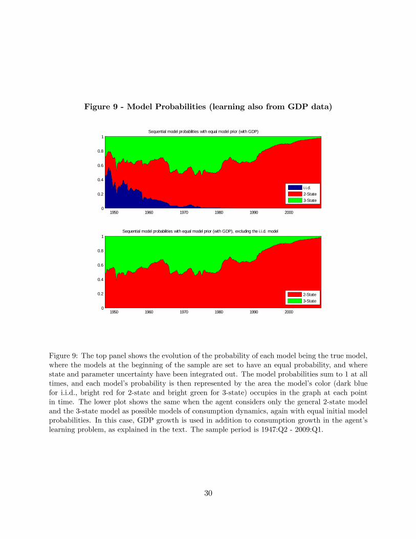
Figure 9 - Model Probabilities (learning also from GDP data)

1950 1960 1970 1980 1990 20000

0.2

0.4

0.6

0.8

1Sequential model probabilities with equal model prior (with GDP)

1950 1960 1970 1980 1990 20000

0.2

0.4

0.6

0.8

1Sequential model probabilities with equal model prior (with GDP), excluding the i.i.d. model

i.i.d.2­State3­State

2­State3­State

Figure 9: The top panel shows the evolution of the probability of each model being the true model,where the models at the beginning of the sample are set to have an equal probability, and wherestate and parameter uncertainty have been integrated out. The model probabilities sum to 1 at alltimes, and each model’s probability is then represented by the area the model’s color (dark bluefor i.i.d., bright red for 2-state and bright green for 3-state) occupies in the graph at each pointin time. The lower plot shows the same when the agent considers only the general 2-state modeland the 3-state model as possible models of consumption dynamics, again with equal initial modelprobabilities. In this case, GDP growth is used in addition to consumption growth in the agent’slearning problem, as explained in the text. The sample period is 1947:Q2 - 2009:Q1.

30

To test this empirically, we regress excess quarterly stock market returns (obtained

from Kenneth French’s web site) on shocks to beliefs about expected consumption growth

and expected consumption growth variance: Et (∆ct+1) − Et−1 (∆ct+1) and σ2t (∆ct+1) −

σ2t−1 (∆ct+1).10 The conditional moments used to generate the regressors integrate out state,

model and parameter uncertainty.

Table 3 - Updates in Beliefs versus Realized Stock Returns

Table 3: The table shows the results from regressions of innovations in agents’ expectations offuture consumption growth (Et+1[∆ct+2]−Et[∆ct+2]) and conditional consumption growth variance(σ2t+1[∆ct+2]−σ2

t [∆ct+2]) versus excess stock market returns. Expectations integrate out parameter,state and model uncertainty, unless otherwise noted. The controls are lagged and contemporaneousrealized log consumption growth, as well as the innovation in expected consumption growth derivedfrom the 3-state model with fixed parameters (i.e., no model or parameter uncertainty), as wellas the i.i.d. model with uncertain parameters. Heteroskedasticity and autocorrelation adjusted(Newey-West; 3 lags) standard errors are reported in paranthesis. ∗ denotes significance at the10% level, ∗∗ denotes significance at the 5% level, and ∗∗∗ denotes significance at the 1% level.The sample is from 1947:Q2 until 2009:Q1. In the below regressions, we have removed the first 40observations (10 years), as a burn-in period to alleviate misspecification of the priors.

Dependent variable: rm,t+1 − rf,t+1 (log excess market returns)1 2 3 4 5 6 7

Et+1 [∆ct+2]− Et [∆ct+2] 40.61∗∗∗ 32.42∗∗ 55.49∗∗∗ 37.27∗∗∗

(8.75) (12.28) (17.00) (10.51)σ2t+1 [∆ct+2]− σ2

t [∆ct+2] −40.73∗∗∗ −18.30(11.13) (11.55)

Controls:

∆ct+1 0.92 3.24∗∗

(1.71) (1.42)∆ct 2.60∗ 2.17

(1.43) (1.44)

[Et+1 [∆ct+2]− Et [∆ct+2]]3-state modelθ known 23.75∗∗∗ −12.63(7.59) (10.66)[

ln(Pt+1/Dt+1+1

Pt/Dt

)]3-state modelθ known

8.44

(11.03)

R2adj 10.0% 11.7% 5.9% 10.0% 9.8% 6.3% 9.9%

10Following Campbell (2003), we use the beginning-of-period timing convention to deal with the time-averaging feature of macro data (see Working (1960), Grossman, Melino, and Shiller (1987), and Breeden,Gibbons, and Litzenberger (1989)). Thus quarterly consumption is assumed to flow at the beginning andnot end of the quarter. When relating consumption growth to stock market returns and consistent withminor lags in consumption responses, Campbell (2003) shows the correlation is higher using beginning ofperiod flows, which we also find.

31

Specifications 1 and 2 in Table 3 show that shocks to expected conditional consumption

growth from the full learning model are positively and strongly significantly associated with

excess stock returns. Crucially, this result holds controlling for contemporaneous and lagged

consumption growth, and thus the results do not simply reflect the fact that realized, con-

temporaneous consumption growth (a direct cash flow effect) was, for example, unexpectedly

high. Thus, revisions in beliefs are significantly related to realized excess returns, consistent

with the learning story.

These results could be driven by state learning. Specification 3 shows that the updates in

expected consumption growth derived from the 3-state model with fixed parameters (that is,

a case with state learning only) are also significantly related to realized stock returns. The

R2, however, is half of that obtained for the full learning model. When revisions in beliefs

from both specifications (with and without parameter learning) are in the regression (spec-

ification 4), the updates in expected consumption growth from the fixed parameters model

are insignificant and have the wrong sign, while belief revisions from the full learning model

remain significant. The same results hold using the 2-state model with fixed parameters

as a control. Thus, updates in expectations derived from learning about about parameters,

states, and models are significantly and positively related to realized stock market returns,

controlling for the updates generated by a model with hidden states and fixed parameters.11

This result is driven by the nonlinear process of jointly learning about parameters and

states. However, returns will in general be a nonlinear function of the updates in beliefs, also

in the case with only state uncertainty. To control for this possible effect, specification 5 adds

the change in the price-dividend ratio as it appears in returns for the fixed parameter model

(with preference parameters that are standard and will be discussed in the next section)

as a control. Again, the “full” learning case dominates that of the model with only state

learning. In sum, the beliefs generated from a model with fixed parameters, a traditional

full-information or ‘rational expectations’model with respect to the parameters, is rejected

when compared to a specification with learning about parameters, models, and states.

Specifications 6 and 7 in Table 3 show that beliefs about shocks to consumption variance

are significantly negatively related to stock returns, as expected if the elasticity of intertem-

poral substitution is above one, as we will assume later in the paper. This result is not

11The updates in beliefs in these regressions are with respect to consumption growth in the near future.These shocks are very highly correlated with shocks to beliefs about long-run consumption dynamics (>0.9)and therefore we unfortunately do not have power to distinguish between long-horizon and short-horizonshocks in our setup. In fact, all the results would go through at the same significance levels if we insteadused long-horizon consumption growth.

32

significant at the 5% level when including contemporaneous and lagged consumption growth

in the regressions (specification 7). This does not mean there is no effect; we just cannot

distinguish it from the direct cash flow effect when learning exclusively from consumption

data.

Table 4 shows the regressions of stock returns and updates in agent beliefs about condi-

tional expected consumption growth and consumption growth variance when including GDP

growth as a source of additional information. The results are similar, but in fact are overall

stronger than results using only historical consumption growth. Updates in agent expecta-

tions about both the first and second moment of consumption growth from the full learning

model are significantly related to stock returns, also after controlling for contemporaneous

and lagged consumption growth and updates in expected consumption growth derived from

a model with fixed parameters.

To summarize, there is strong evidence that updates in beliefs from our full learning

model are significantly related to stock market returns– a particularly stringent test of the

importance of parameter learning about macro dynamics. It is important to recall that no

asset price data was used to generate these belief revisions. This highlights the special and

significant role played by learning in realistic settings and, moreover, questions the common

‘rational expectations’approach, which assumes that agents have full knowledge of the model

specification as estimated using the full sample.12

4.2 Alternative prior beliefs

We also consider a number of alternative priors. In the Online Appendix, we report results

from a model where the mean prior beliefs as of 1947Q1 are equal to maximum likelihood

estimates using data from 1947Q1 to 2009Q1. Thus, this ‘look-ahead’prior incorporates

future information and thus captures the notion that investors, using perhaps a combination

of economic theory and additional data, correctly estimated the most likely parameters

for the postwar sample. The prior standard deviation of beliefs, however, accommodates

parameter and model uncertainty as before. Again, we use the first 10 years, from 1947

through 1956, as a prior ‘burn-in’period. While quantities change somewhat, the overall

12This is a subtle point. In terms of the pricing implications, the learning model is isomorphic to a modelwhere agents know the parameters and the model specification and where the consumption growth dynamicsare assumed to be the same as the subjective dynamics that we estimate from the learning problem. However,the highly non-linear, non-stationary aspects of learning lead to dynamics that we typically would not, andin many cases even could not, otherwise write down.

33

Table 4 - Updates in Beliefs versus Realized Stock Returns (GDP)

Table 4: The table shows the results from regressions of innovations in agents’expectations of fu-ture consumption growth (Et+1[∆ct+2]−Et[∆ct+2]) and conditional consumption growth variance(σ2t+1[∆ct+2]−σ2

t [∆ct+2]) versus excess stock market returns. Expectations integrate out parameter,state and model uncertainty, unless otherwise noted. The controls are lagged and contemporane-ous realized log consumption growth, as well as the innovation in expected consumption growthderived from the 3-state model with fixed parameters (i.e., no model or parameter uncertainty).Both consumption and GDP data is used to estimate the models, as described in the main text.Heteroskedasticity and autocorrelation adjusted (Newey-West; 3 lags) standard errors are reportedin paranthesis. ∗ denotes significance at the 10% level, ∗∗ denotes significance at the 5% level, and∗∗∗ denotes significance at the 1% level. The sample is from 1947:Q2 until 2009:Q1. In the belowregressions, we have removed the first 40 observations (10 years), as a burn-in period to alleviatemisspecification of the priors.

Dependent variable: rm,t+1 − rf,t+1 (log excess market returns)1 2 3 4 5 6

Et+1 [∆ct+2]− Et [∆ct+2] 31.16∗∗∗ 28.42∗∗∗ 34.15∗∗∗ 29.43∗∗∗

(6.15) (7.97) (8.34) (6.85)σ2t+1 [∆ct+2]− σ2

t [∆ct+2] −48.39∗∗∗ −38.66∗∗∗

(8.72) (10.84)Controls:

∆ct+1 0.08 1.23(1.51) (1.52)

∆ct 2.09 2.58∗

(1.32) (1.38)

[Et+1 [∆ct+2]− Et [∆ct+2]]3-state modelθ known −4.75(6.79)[

ln(Pt+1/Dt+1+1

Pt/Dt

)]3-state modelθ known

7.90

(9.94)

R2adj 14.2% 14.7% 13.9% 14.0% 10.9% 13.0%

patterns and conclusions are the same as before when considering belief dynamics from 1957

to 2009. Thus, the results we present in this paper are mainly due to the specific time-series

of shocks realized in the postwar sample, as opposed to something specific to those generated

from priors trained on historical data. An earlier version of this paper also considered priors

with substantially larger prior uncertainty, which captures a higher degree of uncertainty

over the location of the parameters. The results from this case are, again, qualitatively and

quantitatively similar.

In terms of the model probabilities, centering the priors at their post-WWII estimated

values or using larger prior uncertainty in 1947 both lead to a higher likelihood of the 3-

34

state model as the crisis state is not in expectation as severe in these cases from 1957 and

on. Thus, as argued earlier, the model probabilities of the 3-state model are conservative

relative to alternative prior specifications. Overall, however, the conclusions of the paper do

not hinge on the particular priors used– they are robust to reasonable variations in the prior

specifications.

5 Asset pricing implications in general equilibrium

The previous results show that the sequential updates in beliefs are significantly correlated

with realized equity returns. This section provides a formal asset pricing framework to quan-

tify the asset pricing implications for an agent who solves these realistic, high-dimensional,

sequential learning problems using postwar aggregate macro data. In particular, we are

interested in understanding if learning can explain some of the well-documented puzzling

features of the postwar experience, such as a high equity premium, excess return volatility,

excess return predictability, and a high volatility of the price-dividend ratio.

Theoretically, asset pricing in a world with unknown parameters, states, and models is

straightforward, as the agent’s expected utility and asset pricing relevant quantities like the

price-dividend ratio and the ex-ante equity premium are just functions of the overall state of

the economy. The state of the economy is the posterior distribution of the parameters, states,

and models. To solve this problem, a fully rational agent with Epstein-Zin utility needs to

take into account the fact that the agent will revise her beliefs in the future. This requires

calculating all possible belief configurations into the indefinite future. Such a calculation is

prohibitively computationally expensive due to the curse of dimensionality. In our general

setting with parameter and model learning, the joint posterior distribution over parameters,

states, and models is not a known analytical function of the data and, in this case, the pricing

problem for an Epstein-Zin agent is infinite-dimensional. This is true even in the case of a

2-state model with unobserved states and parameters.

Given this, we assume the agent uses an “anticipated utility”approach, originally sug-

gested in Kreps (1998) and previously applied in asset pricing settings with learning by

Sargent and Cogley (2008, 2009) and Piazzesi and Schneider (2010). Kreps suggests this

approach when economic agents are faced with the dual problems of estimating parameters

and models and making decisions/pricing assets in a dynamic setting. The interaction of

the estimation and pricing make these problems horribly complex– so complex, in fact, that

it is diffi cult to believe that economic agents could or would solve such a problem. Instead,

35

Kreps argues agents maximize utility at each point in time assuming the current parameter

estimates and model probabilities are the true parameters, but the agents than updates the

estimates when new data arrives. Thus, the agent is ‘rational,’in that they maximize ex-

pected utility and estimate models/parameters using sophisticated econometrics, but due to

computational constraints, they do not account for the fact that their estimates will change

in the future. In Kreps’s view, this is not a researcher’s short-cut, but rather a normative

theory of how agents compute utility when confronted with complex decisions dependent

on parameter estimates and models. This is the dominant paradigm in macroeconomics for

dealing with parameter uncertainty in a dynamic setting.

While parameter and model uncertainty are not priced risk factors in this framework, they

are nonetheless important for the time-series of asset prices as updates in mean parameter

and model beliefs lead to changes in prices. We do integrate out state uncertainty in the

pricing exercise, so state uncertainty is still a priced risk factor (as in, e.g., Lettau, Ludvigson,

and Wachter (2008)). The anticipated utility approach reduces the number of state variables

to three in the full learning model (the belief about the state in the general 2-state model,

and the 2-dimensional belief about the state in the 3-state model). This approach allows us

to focus on how changes in beliefs arising from the full, high-dimensional learning problem

translate into observable asset returns, return volatilities, and price-dividend ratios.

Later, we characterize asset prices in a simplified 2-state model with unknown parameters,

but known states, where the agent takes parameter uncertainty into account ex-ante. Solving

this simplified model requires GPU parallel computing and a very high level of programming

sophistication. More realistic and higher dimensional problems are well outside the bounds

of computing capabilities.

5.1 Preferences and dividends

Consider a representative agent with Epstein and Zin (1989) preferences, defined recursively

as:

Ut =

{(1− β)C

1−1/ψt + β

(Et[U1−γt+1

]) 1−1/ψ1−γ

} 11−1/ψ

, (3)

where Ct is consumption, ψ 6= 1 is the elasticity of intertemporal substitution (EIS), and

γ 6= 1 is relative risk aversion. These preferences imply the stochastic discount factor:

Mt+1 = β

(Ct+1

Ct

)−γ (βPCt+1 + 1

PCt

) 1/ψ−γ1−1/ψ

, (4)

36

where PCt is the wealth-consumption ratio– that is, the price-dividend ratio for the claim

to the stream of future aggregate consumption. The first component of the pricing kernel

is common to standard power utility preferences, while the second component is present if

the agent has a preference for the timing of the resolution of uncertainty (i.e., if γ 6= 1/ψ).

Given that the consumption dynamics are not ex post calibrated but estimated sequentially,

we also do not calibrate preference parameters to match any particular moment(s). Instead,

we simply use the preference parameters in the main calibration in Bansal and Yaron (2004):

γ = 10, ψ = 1.5, and β = 0.998ˆ3. As mentioned earlier, we consider first an anticipated

utility approach to the pricing problem in terms of parameter and model uncertainty, while

state uncertainty is priced. This corresponds to a world where investors understand and

account for business cycle fluctuations, but where they simply use their best guess for the

parameters governing these dynamics.

The model is solved numerically through value function iteration at each time t in the

sample, conditional on the mean parameter beliefs at time t, which gives the time t asset

prices. The state variables when solving this model are the beliefs about the hidden states

of the economy for each model under consideration. For a detailed description of the model

solution algorithm, please refer to the Online Appendix.

Following both Bansal and Yaron (2004) and Lettau, Ludvigson, and Wachter (2008), we

price a levered claim to the consumption stream with a leverage factor λ of 4.5. The annual

consumption volatility over the postwar sample is only 1.34%, and so the systematic annual

dividend volatility is therefore about 6%. Quarterly log dividend growth is defined as:

∆dt = µ+ λ (∆ct − µ) + εd,t, (5)

where εd,ti.i.d.∼ N

(−1

2σ2d, σ

2d

)is the idiosyncratic component of dividend growth. σd is chosen

to match the observed annual 11.5% volatility of dividend growth reported in Bansal and

Yaron (2004). With these choices of λ and σd we also in fact closely match the sample

correlation they report between annual consumption and dividend growth (0.55).13

13The dividend dynamics imply that consumption and dividends are not cointegrated, which is a com-mon assumption (e.g., Campbell and Cochrane (1999), and Bansal and Yaron (2004)). One could imposecointegration between consumption and dividends, but at the cost of an additional state variable. Further,it is possible to also learn about λ and σ2d. However, quarterly dividends are highly seasonal, which wouldseverely complicate such an analysis. Further, data on stock repurchases are mainly annual. We leave arigorous treatment of these issues to future research.

37

5.2 Empirical results

5.2.1 Unconditional moments

Table 5 reports realized asset pricing moments in the data, as well as those generated by

the learning models over the same sample period. The models with parameter uncertainty

match the sample equity premium reasonably well: 4.7% in the data versus 3.7% for the

full model with parameter and model uncertainty when learning from consumption data

only, and 5.2% for the full model with learning from both consumption and GDP data. The

models using GDP as an additional signal have a more severe recession state, which explain

higher average equity returns. Models with fixed parameters generate very small sample

equity premiums 1.1% and 1.7% for the 2- and 3-state models, respectively. Thus, allowing

for parameter and model uncertainty more than triples the sample risk premiums, despite

the fact that parameter and model uncertainty are not priced risk factors under anticipated

utility pricing.

The source of differences in equity premiums between the fixed and unknown parameters

cases can be seen from sample average ex ante equity risk premiums (ET[E(Rexcessm,t+1 |It

)],

where It denotes the information set (beliefs) of agents at time t and ET [·] denotes the sampleaverage). Since parameter and model uncertainty are not priced risks with anticipated utility,

one may expect the average ex ante risk premiums to be similar to the corresponding model

with known parameters. However, for the 2-state model with parameter uncertainty and

learning from consumption only, for instance, the average ex ante sample risk premium is

1.8%, whereas the average ex ante sample risk premium for the 2-state model with known

parameters is 0.9%. A similar difference is present between the 3-state models. Through the

postwar period, the agent learns that expansions are longer, recessions milder than initially

thought, and volatility is lower than previously thought. This leads to a higher ex ante risk

premium early in the sample. At the end of sample, on the other hand, the conditional risk

premium of the models with parameter uncertainty is lower and similar to that of the fixed

parameters models.

These unexpected, overall positive surprises in belief updates not only decrease the ex

ante risk premium over the sample, but also increases the price-dividend ratio. Thus, ex

post average returns are higher than the ex ante expected returns, explaining the remaining

difference between the sample risk premium with parameter and model learning versus the

fixed parameter case. Fama and French (2002) reach a similar conclusion in terms of the ex

post versus the ex ante risk premium when looking at the time-series of the aggregate price-

38

Table5-AssetPriceMom

ents

Table5:ThetablereportstheassetpricingimplicationsofthemodelswithananticipatedutilityversionoftheEpstein-Zin

preferencesunderdifferentpriors,aswellasthefixedparameterscases.Forallthemodels,γ

=10,β

=0.

994,ψ

=1.

5,λ

=4.

5.Thevolatilityoftheidiosyncraticcomponentofdividendgrowth(εd,t)iscalibratedtomatchthehistoricalstandarddeviation

ofdividendgrowth,asreportedinBansalandYaron(2004).Thestatisticsareannualized.TheexpectationoperatorwithaT

subscript,ET,denotesthesampleaverage,whilethevolatilityoperator,σTdenotesthesamplestandarddeviation.Thesample

periodisfrom

1957:Q2until2009:Q1,with1957Q1priorsasgiveninTable1forthecaseoflearningfrom

observingconsumption

growthonly,andasgiveninanOnlineAppendixforthecaseoflearningfrom

bothconsumptionandGDPgrowth.

Data

Learningfrom

consumption

Learningfrom

cons.&GDP

Knownparameters

1957:Q2-

Full

i.i.d.

2-state

3-state

Full

i.i.d.

2-state

3-state

2-state

3-state

Moments

2009:Q1

model

model

model

model

model

model

model

model

model

model

Therealrisk-freerate:

ET

(rf t)

1.6

%3.7

%3.7

%3.7

%3.5

%3.5

%3.8

%3.5

%3.4

%3.8

%3.7

%

σT

(rf t)

1.6

%0.7

%0.3

%0.8

%1.0

%1.1

%0.2

%0.9

%1.4

%0.6

%0.9

%

Thedividendclaim:

∆dt

=µ

+λ

(∆c t−µ

)+ε d,t

expost:

ET

(rt−rf t

)4.7

%3.7

%2.9

%3.7

%6.0

%5.2

%2.6

%5.2

%6.7

%1.1

%1.7

%

σT

(rt−rf t

)17.1

%15.1

%14.5

%15.2

%14.1

%14.9

%14.9

%14.2

%15.3

%11.9

%12.2

%Sharperatio

0.2

70.2

50.2

00.2

40.4

30.3

50.1

70.3

70.4

40.0

90.1

4σT

(pdt)

0.3

80.2

20.2

40.2

30.2

10.2

30.3

10.2

50.1

50.0

60.0

7

Corr T

(pdModel

t,pdData

t)

n/a

0.4

20.2

80.3

90.5

00.6

70.3

50.4

30.6

20.2

50.2

6

exante:

ET

[Et(rt+

1−rf t

+1)]

n/a

1.8

%1.4

%1.8

%3.2

%3.2

%1.4

%2.4

%5.2

%0.9

%1.5

%

39

earnings and price-dividend ratios. Our results are consistent with theirs, but our models

are estimated from macro fundamentals alone.

Learning generates additional volatility in equity returns and the price-dividend ratio.

Equity return volatility in the parameter and model uncertainty cases are about 15%, close

to the 17% annual return volatility in the data. In contrast, equity return volatility in the

models with fixed parameters is about 12%, only slightly higher than the annual dividend

growth volatility (11.5%). Thus, sample variation in discount and expected dividend growth

rates arising from belief updates cause excess return volatility (Shiller (1980)), through a

volatile price-dividend ratio. The sample volatility of the log price-dividend ratio is 0.38

in the data and is only 0.06 − 0.07 in the fixed parameter cases. With parameter/model

learning, the log price-dividend ratio volatility is 0.25 (depending somewhat of the exact

model specification), which is four times the values observed with fixed parameters.14 This

is exactly what one would expect, as learning generates shifts and drifts in parameters that

have a first order impact on price-dividend ratios.

We also find a high correlation between our learning model implied log price-dividend

ratios and those in the data: 0.67 for the full learning model estimated with both GDP

and consumption and 0.42 for the full learning model using only consumption. Of the

individual models, the dividend-price ratio from the 3-state model has highest correlation

with its observed counterpart. Thus, even though the 3-state model has a very low model

probability towards the end of the sample (see Figure 3), it is important for pricing. In

fact, the full learning specification with model uncertainty has a higher correlation between

the dividend-price ratio from the model and the data than any of the individual, underlying

models, with the iid model having the lowest correlation.

The fixed parameter models have lower correlations, 0.25 for the 2-state model and 0.26

for the 3-state model. Thus, the covariance between the price-dividend ratio in the data and

the full learning model using both consumption and GDP growth is roughly 30 times higher

than the highest covariance between the price-dividend ratio in the data and the models

with fixed parameters (0.0354 vs. 0.0013). Overall, parameter/model learning generates a

time-series of the aggregate stock market price level (normalized by dividends) that much

more closely match the observed data than models with fixed parameter models.

14The price-dividend ratio in each model is calculated as the corresponding in the data by summing thelast four quarters of payouts to get annual payout. The price-dividend ratio from the data includes sharerepurchases in its definition of total dividends.

40

5.2.2 The time-series of asset prices

To further understand how our learning models match the aggregate stock price level (the

log dividend-price ratio), we regress the dividend-price ratio in the data on the dividend-

price ratios implied by the different models, both in levels and in changes. This allows to

separately identify the effect of state learning (in models with fixed parameters) from the

effect of parameter and model learning (in models with unknown states, parameters, and

models).

Panel A of Table 6 summarizes the level regressions. The anticipated utility model with

learning about both parameters and models from both consumption and GDP data provides

the best ‘fit.’This model has an R2 of 46% and one cannot reject a zero intercept and slope

of one. The dividend-price ratio generated by the fixed parameter model is insignificant in a

regression that also includes the full-learning model. Even though the 2-state model quickly

dominates in terms of model probabilities, the model-averaged specification has additional

explanatory power relative to the 2-state model. This occurs as the 3-state model’s depression

state is important for asset prices even though it is quite unlikely. The increase in fit when

going from the fixed parameter models to the full learning models stems from both an

improvement in matching business cycle fluctuations in the dividend yield and a better fit

to low-frequency fluctuations. In particular, with parameter learning the dividend yield

displays a downward trend over the sample, similar to that found in the data as documented

by, for instance, Fama and French (2002).

As a robustness check, Panel B of Table 6 shows the same regressions in differences.

Again, the models with anticipated utility fare the best and are significant, and fixed para-

meter specifications are insignificant. In sum, including parameter and model uncertainty

leads to not only better fit of the unconditional asset pricing moments, but a significantly

better fit of the realized time-path of the aggregate stock price level in the postwar era. The

’full’ learning models with joint learning about states, parameters, and models match the

data best.

5.2.3 Permanent shocks and the volatility of long-run yields

With parameter and model uncertainty, the belief updates constitute permanent shocks to

expectations about consumption growth rates, consumption growth volatility, and higher

order moments. While shocks to a transitory state variable eventually die out, and so

(very) long-run expectations are constant, shocks to, for instance, the mean belief about the

41

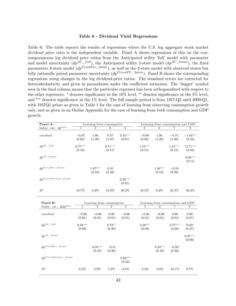
Table 6 - Dividend Yield Regressions

Table 6: The table reports the results of regressions where the U.S. log aggregate stock marketdividend price ratio is the independent variable. Panel A shows regressions of this on the con-temporaneous log dividend price ratios from the Anticipated utility ’full’model with parameterand model uncertainty (dpAU_full), the Anticipated utility 2-state model (dpAU_2state), the fixedparameters 3-state model (dpFixedPar_3state), as well as the 2-state model with observed states butfully rationally priced parameter uncertainty (dpPricedPU_2state). Panel B shows the correspondingregressions using changes in the log dividend-price ratios. The standard errors are corrected forheteroskedasticity and given in parantheses under the coeffi cient estimates. The ’dagger’symbolseen in the final column means that the particular regressor has been orthogonalized with respect tothe other regressors. ∗ denotes significance at the 10% level, ∗∗ denotes significance at the 5% level,and ∗∗∗ denotes significance at the 1% level. The full sample period is from 1957:Q2 until 2009:Q1,with 1957Q1 priors as given in Table 1 for the case of learning from observing consumption growthonly, and as given in an Online Appendix for the case of learning from both consumption and GDPgrowth.

Panel A: Learning from consumption Learning from consumption and GDPIndep. var.: dpdata 1 2 3 4 5 6 7 8

constant −0.87 1.86 0.57 3.44∗∗∗ −0.09 1.86 −0.71 −1.43∗∗∗

(0.64) (1.98) (1.67) (0.91) (0.46) (1.98) (1.40) (0.34)

dpAU_ full 0.77∗∗∗ 0.71∗∗∗ 1.13∗∗∗ 1.15∗∗∗ †2.71∗∗∗

(0.19) (0.17) (0.15) (0.15) (0.33)

dpAU_ 2state 0.68∗∗∗

(0.11)

dpFixedPar_ 3state 1.47∗∗∗ 0.45 1.48∗∗∗ −0.19(0.54) (0.42) (0.54) (0.39)

dpPricedParUnc_ 2state 2.38∗∗∗

(0.31)

R2 18.7% 6.2% 18.8% 46.3% 45.5% 6.2% 45.3% 63.4%

Panel B: Learning from consumption Learning from consumption and GDPIndep. var.: ∆dpdata 1 2 3 4 5 6 7 8

constant −0.00 −0.00 0.00 −0.00 −0.00 −0.00 0.00 0.00(0.01) (0.01) (0.01) (0.01) (0.01) (0.01) (0.01) (0.01)

dpAU_ full 0.34∗∗∗ 0.72∗∗ 0.38∗∗∗ 0.77∗∗∗ †0.83∗

(0.09) (0.30) (0.09) (0.28) (0.47)

dpAU_ 2state 0.37∗∗∗

(0.09)

dpFixedPar_ 3state 0.34∗∗∗ −0.51 0.34∗∗∗ −0.56∗

(0.10) (0.36) (0.10) (0.32)

dpPricedParUnc_ 2state 0.62∗∗∗

(0.22)

R2 6.5% 3.9% 7.2% 3.4% 8.4% 3.9% 10.1% 8.7%

42

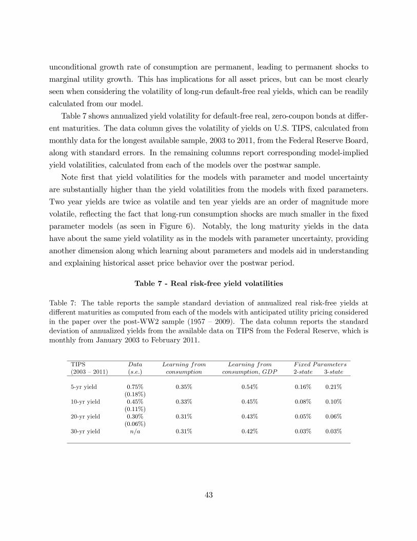
unconditional growth rate of consumption are permanent, leading to permanent shocks to

marginal utility growth. This has implications for all asset prices, but can be most clearly

seen when considering the volatility of long-run default-free real yields, which can be readily

calculated from our model.

Table 7 shows annualized yield volatility for default-free real, zero-coupon bonds at differ-

ent maturities. The data column gives the volatility of yields on U.S. TIPS, calculated from

monthly data for the longest available sample, 2003 to 2011, from the Federal Reserve Board,

along with standard errors. In the remaining columns report corresponding model-implied

yield volatilities, calculated from each of the models over the postwar sample.

Note first that yield volatilities for the models with parameter and model uncertainty

are substantially higher than the yield volatilities from the models with fixed parameters.

Two year yields are twice as volatile and ten year yields are an order of magnitude more

volatile, reflecting the fact that long-run consumption shocks are much smaller in the fixed

parameter models (as seen in Figure 6). Notably, the long maturity yields in the data

have about the same yield volatility as in the models with parameter uncertainty, providing

another dimension along which learning about parameters and models aid in understanding

and explaining historical asset price behavior over the postwar period.

Table 7 - Real risk-free yield volatilities

Table 7: The table reports the sample standard deviation of annualized real risk-free yields atdifferent maturities as computed from each of the models with anticipated utility pricing consideredin the paper over the post-WW2 sample (1957 —2009). The data column reports the standarddeviation of annualized yields from the available data on TIPS from the Federal Reserve, which ismonthly from January 2003 to February 2011.

TIPS Data Learning from Learning from Fixed Parameters(2003 —2011) (s.e.) consumption consumption, GDP 2-state 3-state

5-yr yield 0.75% 0.35% 0.54% 0.16% 0.21%(0.18%)

10-yr yield 0.45% 0.33% 0.45% 0.08% 0.10%(0.11%)

20-yr yield 0.30% 0.31% 0.43% 0.05% 0.06%(0.06%)

30-yr yield n/a 0.31% 0.42% 0.03% 0.03%

43

5.2.4 Excess return forecastability

Next, we consider excess market return forecasting regressions using the dividend yield as the

predictive variable. These regressions have a long history and remain a feature of the data to

be explained by asset pricing models (e.g., Campbell and Cochrane (1999), Bansal and Yaron

(2004)), even if the strength of the empirical evidence is debatable (see, e.g., Stambaugh

(1999), Ang and Bekaert (2007), Boudoukh, Richardson andWhitelaw (2008), and Goyal and

Welch (2008) for critical analyses). We consider standard forecasting regressions overlapping

at the quarterly frequency using model-implied market returns and dividend yields. As

before, we are not looking at population moments or average small-sample moments, but

the single sample generated by feeding the models the actual sample of realized consumption

growth.

Table 8 shows the forecasting regressions over different return forecasting horizons from

the data. We use both the market dividend yield and Lettau and Ludvigson’s (2001) ap-

proximation to the consumption-wealth ratio, cay, to document the amount of predictability

implied by these regressions in the data. We then run the same regressions using model im-

plied returns and dividend yields. The fixed parameters models (bottom right in the table)

generate no significant return predictability at the 5% significance level and the R2’s are very

small. These models do, in fact, feature time-variation in the equity risk premium, but the

risk premium volatility is only about 0.5% per year and so the signal-to-noise ratio in these

regressions is too small to generate significant in-sample predictability.

The models with parameter uncertainty, however, display significant in-sample return

predictability and the regression coeffi cients and the R2’s are large and increasing in the

forecasting horizon similar to those in the data. The ex ante predictability in the models with

anticipated utility pricing is in fact similar to that in the fixed parameters cases, but since

the parameters are updated at each point in time, there is significant ex post predictability.

For instance, an increase in the mean parameter of consumption growth leads to a high

return and lower dividend yield. Thus, a high dividend yield in sample forecasts high excess

returns in sample. This mechanism was previously identified by Timmermann (1993) and

Lewellen and Shanken (2002), and can be understood as a strong form of the Stambaugh

(1999) bias. Thus, the model predicts that the amount of predictability is much smaller

out-of-sample, consistent with the empirical evidence in Goyal and Welch (2008) and Ang

and Bekaert (2007).

44

Table 8 - Return Forecasting Regressions

Table 8: This table presents quarterly excess market return forecasting regressions over variousforecasting horizons (q quarters; 1 to 16). The top left panel shows the results when using marketdata and a measure of the log aggregate dividend yield; the cay-variable of Lettau and Ludvigsson(2001) and the CRSP aggregate log dividend yield (ln Dt

Ptwhere dividends are measured as the sum

of the last four quarters’dividends. The rest of the table shows the results using the returns anddividend yield generated within the models. "Cons. only" denotes the model results in the casewhere only consumption growth is used to update beliefs, while "Cons. and GDP" denotes themodel results in the case where both consumption and GDP growth are used to update beliefs.The results for ’Anticipated E-Z utility’refers to the anticipated utility case of the full model withstate, parameter, and model uncertainty. The ’P.P.U. E-Z utility’results refer to the 2-state modelwith fully rational pricing of the parameter uncertainty where the states are observed. Finally,the fixed parameters case correspond to the case of state uncertainty where the parameters areknown. Newey-West autocorrelation and heteroskedasticity adjusted standard errors are given inparentheses (the number of lags is equal to the number of overlapping observations). ∗ denotessignificance at the 10% level, ∗∗ denotes significance at the 5% level, and ∗∗∗ denotes significanceat the 1% level. The sample period is from 1957:Q2 until 2009:Q1, with 1957Q1 priors as given inTable 1 for the case of learning from observing consumption growth only, and as given in an OnlineAppendix for the case of learning from both consumption and GDP growth.

rt,t+q − rf,t,t+q = αq + βq,dp ln (Dt/Pt) + εt,t+q

Data Anticipated E-Z utility

ln (Dt/Pt) := cayt ln (Dt/Pt) := lnΣ3j=0D

Mkt.t−j

PMkt.t

Cons. only Cons. and GDP

q βdp (s.e.) R2adj βdp (s.e.) R2

adj βdp (s.e.) R2adj βdp (s.e.) R2

adj

1 1.19∗∗∗ 4.67% 0.03∗ 1.6% 0.03 1.0% 0.03 0.8%(0.31) (0.02) (0.03) (0.02)

4 4.29∗∗∗ 15.65% 0.11∗∗ 6.6% 0.18∗∗ 6.4% 0.14∗∗ 5.1%(1.18) (0.05) (0.07) (0.06)

8 7.60∗∗∗ 28.1% 0.17∗ 8.5% 0.37∗∗∗ 14.7% 0.29∗∗∗ 13.4%(1.72) (0.10) (0.10) (0.09)

16 12.31∗∗∗ 41.6% 0.22∗∗ 9.5% 0.59∗∗∗ 20.7% 0.42∗∗∗ 16.6%(1.82) (0.11) (0.16) (0.14)

P.P.U. E-Z utility Fixed parametersγ = 5 γ = 10 2-state model 3-state model

q βdp (s.e.) R2adj βdp (s.e.) R2

adj βdp (s.e.) R2adj βdp (s.e.) R2

adj

1 0.10∗∗ 2.1% 0.12∗∗∗ 3.4% −0.01 0.0% 0.005 0.0%(0.05) (0.04) (0.06) (0.06)

4 0.32∗ 6.0% 0.42∗∗∗ 11.2% 0.19 1.1% 0.21 1.3%(0.17) (0.15) (0.17) (0.16)

8 0.54∗ 9.1% 0.68∗∗ 15.9% 0.40 2.5% 0.44∗ 3.3%(0.32) (0.28) (0.24) (0.23)

16 1.03 12.6% 1.16∗∗ 18.0% 0.29 0.8% 0.32 1.1%(0.73) (0.53) (0.31) (0.31)

45

5.3 Anticipated utility versus priced parameter uncertainty

One potential criticism of the anticipated utility results is that the impact of changing beliefs

would be tempered if the agent took into account that the parameters could change in the

future and properly priced the parameter risk. This section contrasts the results for a model

with fully-priced parameter uncertainty to our anticipated utility specification.

Collin-Dufresne, Johannes, and Lochstoer (2013) provide a detailed study of the impact

of priced parameter uncertainty, develop solution methods, and theoretically quantify the

impact of priced parameter uncertainty in a range of simple models and for various pa-

rameters. They find that priced parameter uncertainty can have quantitatively large and

long-lasting asset pricing effects. Pricing parameter uncertainty dramatically increases the

dimensionality of the pricing problem, however, pushing the bounds of computational limits

even for models with a modest number of parameters. Here, we utilize their pricing approach

and consider a 2-state model with observed states with parameters unobserved. This is the

most general model for which it is computationally feasible to solve for prices. This ignores

the confounding effects we discussed earlier, but insures that the posterior distribution is

summarized by a fixed-dimensional set of suffi cient statistics, which allows the computation

of expected utility. As mentioned earlier, if the Markov state is unobserved, the pricing

problem for an Epstein-Zin agent is infinite-dimensional.

The details of the numerical solution for this exercise are given in the Online Appendix.

The problem is extremely computationally intensive with 9 state variables, where 8 state

variables are needed to characterize the hyperparameters governing parameter beliefs, and

1 state variable is the current state of the Markov chain. We solve the model using parallel

computing techniques on a workstation using a GPU (graphical processing unit) card, effi -

ciently programmed in C++ and Cuda.15 A full learning model including both model and

parameter uncertainty across all models is vastly out of reach given current available comput-

ing power.16 We solve the 2-state model with priced parameter uncertainty for γ = 10, the

same value as used for the anticipated utility models, and γ = 5. Otherwise, the parameters

are the same across the two models.15We run the code on a single computer using in parallell 16 high-speed CPU’s and 1024 lower speed

processors on a GPU card. CUDA programming is required for effi ciently communicating with the GPUcard. Further, the problem requires 96Gb of RAM memory due to the size of the state-space. It takes about2 weeks to solve the model with suffi cient accuracy. Thus, since computing time is exponential, adding evenone more continuous state variable makes the problem computationally infeasible.16It is also prohibitively computationally expensive for us to calculate long-run real yields for the 2-state

model with priced parameter uncertainty, as the yield calculations require additional recursive calculations.

46

We classify the states sequentially based on the mean state beliefs from the 2-state model

with unknown states and parameters, as shown in the middle plot of Figure 1, where state

2 (1) is said to occur if the mean state belief (Et [st]) is above (below) 1.5. Thus, as seen in

Figure 1, every NBER recession except the recessions in 1969-1970 and 2001 are identified

as state 2 observations. This classification thus accounts for parameter uncertainty. The

parameter priors are the same as those used earlier, as described in Table 1.

Table 9 summarizes the results. Average excess returns increase with priced parameter

uncertainty, from 3.7% for the 2-state model with anticipated utility to 7.5% for the case

with priced parameter uncertainty. With γ = 5 the risk premium is close to that in the

data (4.6%) . The average ex ante sample risk premiums for γ = 5 or 10 are 5.6% and

2.5%, respectively, compared to 1.8% for the anticipated utility case. Two observations are

warranted. First, ex ante risk premiums are much higher with priced parameter uncertainty.

This is due to the permanent shocks to beliefs about consumption dynamics arising from

parameter belief updates. These long-run shocks are priced risks when the agent has a

preference for early resolution of uncertainty, as explained in Collin-Dufresne, Johannes,

and Lochstoer (2013). For instance, an update in the mean belief about the growth rate

of either of the states (µ1 or µ2) will cause an upward revision in the wealth-consumption

ratio. From the stochastic discount factor, as given in Equation (4), this corresponds to a

negative shock to the pricing kernel. This is similar to the mechanics in the Bansal and

Yaron (2004) model. Second, a large fraction of the realized average equity returns are due

to unanticipated positive shocks, as observed in the difference between the average realized

excess returns versus the average expected excess returns (ET[E(Rexcessm,t+1 |It

)]). However, the

fraction is a little smaller than for the anticipated utility cases. This occurs since discount

rates are higher with priced parameter uncertainty, which in turn means that the shocks

to the growth rate affects the price-dividend ratio less, causing more muted updates in the

price level.

In terms of volatilities, return volatility and the volatility of the price-dividend ratio

are lower than in the anticipated utility case, due to the same effect– discount rates are

higher ex ante with priced parameter uncertainty. The correlation between the model-

implied and observed price-dividend ratios is higher for 2-state model with priced parameter

uncertainty, than for the same model with anticipated utility case or with fixed parameters.

The correlation in the full learning model was 0.67, and is comparable to the case with priced

parameter uncertainty.

47

Table9-Priced

param

eteruncertain

tyvs.Anticip

atedutility

:

Theasset

price

mom

ents

Table

9:Thetable

reports

theasset

pricingimplications

ofthe2-state

Markov

switching

regimemodelfor

different

assumptions

oninvestors

information

set,aswellasthe

pricingmethodology.

Inparticular,

’P.P.U.E-Z’stands

forpriced

parameter

uncertaintyEpstein-Z

inutility,

andcorresp

ondstothe

fullyrational

casewhere

investorsaccount

forthe

parameter

uncertaintyexante

inthe

pricingofasset

claims.Inthis

case,the

stateisassum

edtobeobserved.

’Anticipated

E-Z’corresp

ondstothe

anticipatedutility

Epstein-Z

inagent

asgiven

inTable

5,where

theagent

ateach

point

intimeprices

assetsusing

theircurrent

best

guessofthe

parameters

asthe

trueparam

etervalue.

Inthis

casethe

stateisunobserved,

andthe

agenttakes

intoaccount

stateuncertainty

when

pricingthe

claim.Finally,

’Know

nparam

eters’corresp

ondtothe

casewhere

parameters

areknow

nbut

where

thestate

isunobserved

butthere

isnoparam

eteruncertainty,

alsoreproduced

fromTable

5.Inallcases,

theagent

learnsfrom

observingconsum

ptiongrow

thonly.

Forallthe

models,

γ=

10,β

=0.994,

ψ=

1.5,

λ=

4.5.

Thevolatility

ofthe

idiosyncraticcom

ponent

ofdividend

growth(εd,t )iscalibrated

tomatch

thehistorical

standarddeviation

ofdividend

growth,

asreported

inBansal

andYaron

(2004).Thestatistics

areannualized.

Theexp

ectationoperator

with

aTsubscript,

ET,denotes

thesam

pleaverage,

while

thevolatility

operator,

σTdenotes

thesam

plestandard

deviation.Thesam

pleperiod

isfrom

1957:Q2until

2009:Q1,with

1957Q1priors

asgiven

inTable

1for

thecase

oflearning

fromobserving

consumption

growthonly,

andasgiven

inanOnline

Appendix

forthe

caseoflearning

fromboth

consumption

andGDPgrow

th.

Data

P.P.U.E-Z

P.P.U.E-Z

Anticipated

E-Z

Know

nparam

eters1957:Q

2-2-state

model

2-statemodel

2-statemodel

2-statemodel

Moments

2009:Q1

γ=

5γ

=10

γ=

10γ

=10

Thereal

risk-freerate:

ET

(rft)

1.6%3.6

%3.0

%3.7

%3.8%

σT

(rft)

1.6

%0.9

%1.3

%0.8

%0.6%

Thedividend

claim:

∆dt

=µ

+λ

(∆ct −

µ)

+εd,t

expost:

ET

(rt −

rft)

4.7%

4.6

%7.5

%3.7

%1.1%

σT

(rt −

rft)

17.1

%13.8

%13.8

%15.2%

11.9%

Sharperatio

0.27

0.34

0.54

0.24

0.09σT

(pdt )

0.38

0.11

0.11

0.23

0.06Corr

T(pdModel

t,pdData

t)

n/a

0.62

0.69

0.39

0.25

exante:

ET

[Et (r

t+1 −

rft+1 )]

n/a

2.5

%5.6

%1.8

%0.9%

48

5.3.1 Conditional Moments

Figure 10 displays the time-series of the conditional risk premium and Sharpe ratio for

the 2-state model with anticipated utility pricing as well as the 2-state model with priced

parameter uncertainty (where the state is assumed to be observed). The latter has a strongly

counter-cyclical risk premium and Sharpe ratio, due to the higher parameter uncertainty in

recessions. Of particular importance, as shown in Collin-Dufresne, Johannes, and Lochstoer

(2013), is the uncertainty about the transition probabilities. These parameters govern the

persistence of the consumption growth process– an aspect of consumption dynamics that an

Epstein-Zin agent with a preference for early resolution of uncertainty finds particularly risky.

Table 1 shows that the uncertainty about transition probabilities remain large throughout

the sample. The anticipated utility model also has a countercyclical risk premium and Sharpe

ratio, though the magnitude is smaller as the ex ante priced risk in this case is related only

to the known dynamics within a state as well as the state uncertainty.

The lower left quadrant of Table 8 shows forecasting regressions for the case with priced

parameter uncertainty in the 2-state model. Although there is more ex ante variation in

discount rates, as seen in Figure 10, there is less of a response in the dividend price ratio

to belief updates, due to the higher average discount rate, as discussed in an earlier section.

Thus, fully rational pricing decreases the in-sample evidence of predictability due to ex post

revisions in beliefs, but in turn has more actual variation in the risk premium. In fact, the

predictability evidence is strongest for the high risk aversion case (γ = 10), which exhibits

very high time-variation in the ex ante conditional risk premium.

5.3.2 Discussion

In terms of robustness, the main difference between anticipated utility and priced parameter

uncertainty is that the former generates more return and dividend-price volatility, and the

latter higher ex-ante risk premiums. Both approaches generate a large difference between

the ex ante and ex post risk premium, excess return volatility, return predictability, and a

higher correspondence to the time-series of the price-dividend ratio in the data than the fixed

parameters benchmark models. It is important to note that none of the results in Sections 2

and 3 depend on whether we use anticipated utility or fully price the parameter uncertainty,

thus of all the main empirical results are robust to priced parameter uncertainty, at least

for the 2-state model. Cogley and Sargent (2009) find similar results in a number of simple

macroeconomic models.

49

Figure 10 - Anticipated utility vs. priced parameter uncertainty:Conditional risk premium and Sharpe ratio in the 2-state model

1957 1967 1977 1987 1997 20070

0.02

0.04

0.06

0.08

0.10

0.12Annualized conditional  risk premium

Year

Ris

k pr

emiu

m

1957 1967 1977 1987 1997 20070

0.1

0.2

0.3

0.4

0.5

0.6Annualized conditional  Sharpe ratio

Year

Shar

pe ra

tio

Anticipated util i tyPriced parameter uncertainty

Anticipated util i tyPriced parameter uncertainty

Figure 10: The top plot shows the annualized conditional risk premium on the dividend claim fromthe 2-state model with anticipated utility pricing (the black, solid line), as well as the case wherethe parameter uncertainty is fully rationally priced, but the state is assumed to be observed (thered, dashed line). In the former case, the risk aversion parameter γ = 10, whereas in the latter caseγ = 5, such that the average risk premium over the sample is similar in both models. The sampleperiod is 1957:Q2 - 2009:Q1. The bottom plot shows the annualized conditional Sharpe ratio ofreturns to the dividend claim for the same two cases over the same sample period.

50

Priced parameter uncertainty requires a number restrictive assumptions. Most notably, it

requires that states are observed which precludes the strong confounding effects documented

earlier in Table 2. Parameter learning is much slower with unobserved states, thus the 2-

state model with priced parameter uncertainty omits an important source of confounding

risk that substantially affects the belief updating process.

Overall, although priced parameter uncertainty is certainly realistic and a powerful pric-

ing mechanism, there are also good reasons to believe that economic agents engage in ‘antic-

ipated utility’-type pricing along some dimensions. First, as suggested by Kreps (1998), this

appears to be the way that economists approach diffi cult pricing problems with non-trivial

parameter estimation. Second, since joint parameter and state learning is a realistic feature of

the data and since anticipated utility in this case is required to generate a finite-dimensional

pricing problem, this also suggests the practicality of an anticipated utility approach. To

our knowledge, there are no known methods for truly infinite dimensional pricing problems.

Third, we also find that the covariance between the price-dividend ratio in the data and the

price-dividend ratio of the models with anticipated utility pricing are substantially higher

than the covariance between the price-dividend ratio in the data and the price-dividend ratio

from the model with priced parameter uncertainty.

6 Conclusion

This paper empirically studies the impact of parameter and model uncertainty on US postwar

equity returns in the context of standard consumption based asset pricing models, and

contributes to a growing empirical literature documenting the importance of learning for

asset prices (see Pastor and Veronesi (2009) for a review article).

We take the perspective of a Bayesian agent who learns from macroeconomic data about

consumption dynamics, updating beliefs as new data arrives. If structural learning is an im-

portant determinant of the US postwar experience, three conditions should hold. First, the

agent’s subjective beliefs generated from learning should be substantially different from those

arising from traditional implementations of similar models. Second, when beliefs change, so

should asset prices: thus belief updates should be significantly correlated with market re-

turns. Third, these beliefs, when embedded in an equilibrium asset pricing model, should

help us understand the standard asset pricing puzzles: the realized high equity premium, ex-

cess return volatility, excess return predictability, and a volatile price-dividend ratio. We find

strong evidence along all three dimensions, supporting the empirical relevance of structural

51

learning.

Parameter and model learning generates subjective beliefs that are nonstationary over

time, and this, in turn generates large shocks to beliefs about long-run consumption dy-

namics. These long run beliefs have first order asset pricing implications for agents with

Epstein-Zin preferences (see, e.g., Bansal and Yaron (2004)). We also find that the largest

shocks to long-run beliefs occur during recessions, as agents update their views about diffi -

cult to estimate parameters. Over the sample, agents learn that consumption dynamics are

less risky: shorter recessions, longer expansions, and lower volatility, which generates higher

ex post equity returns than those expected ex-ante.

These results have a number of implications. First, we find an alternative narrative for

US postwar equity experience: macroeconomic learning is an important component of equity

returns helps to explain the high realized equity returns, high equity volatility relative to

fundamentals, return predictability, and the time series of price-dividend ratios. Second, the

evidence suggests that expected equity returns going forward is substantially lower than the

historical average excess returns, which has first important implications for long-run portfolio

investment and capital budgeting decisions. Third, looking forward, there is still substantial

uncertainty over parameters associated with recessions/depressions and future data could

dramatically change beliefs over these states.

Our results and methodology can be extended in a number of ways. First, it would be

useful to use our methods to understand the experience of other countries through the lens of

learning about macroeconomic fundamentals. In particular, the macroeconomic and equity

market experiences of Japan are dramatically different, and it would interesting to study

how agent’s macroeconomic beliefs have evolved over time. Second, we assume learning

without structural breaks. For many countries, structural shifts like currency devaluations,

bailouts, or shifts in central bank policies may be important, which could ‘re-start’struc-

tural learning. Our approach can easily be modified to handle this case. Finally, there is

strong evidence for cross-sectional heterogeneity in agents’asset holdings and consumption

dynamics. These effects would likely introduce additional asset pricing implications when

combined with learning effects. We leave these topics for future research.

References

[1] Ai, H. (2010), “Information about Long-Run Risk: Asset Pricing Implications,”forth-

coming, Journal of Finance.

52

[2] Ang, A. and G. Bekaert (2007), “Return predictability: Is it there?”, Review of Financial

Studies, 20, 3, 651-707.

[3] Backus, D., M. Chernov and I. Martin (2009), “Disasters Implied by Equity Index

Options”, NYU Working Paper

[4] Bakshi, G. and G. Skoulakis (2010), “Do Subjective Expectations Explain Asset Pricing

Puzzles?”, Journal of Financial Economics, December 2010, 117 - 140.

[5] Bansal, R. and A. Yaron (2004), “Risks for the Long-Run: A Potential Resolution of

Asset Pricing Puzzles”, Journal of Finance 59(4), 1481 - 1509

[6] Bansal, R. and I. Shaliastovich (2010), “Confidence Risk and Asset Prices,”American

Economic Review P&P, 100, 537 —541.

[7] Barberis, N. (2000), “Investing for the Long Run When Returns Are Predictable”,

Journal of Finance 55(1), 225 - 264

[8] Barillas, F., Hansen, L. and T. Sargent, “Doubts or Variability?”, Journal of Economic

Theory, forthcoming.

[9] Barro, R. (2006), “Rare Disasters and Asset Markets in the Twentieth Century”, Quar-

terly Journal of Economics 121, 823 - 866

[10] Barro, R., Nakamura, E., Steinsson, J., and J. Ursua (2009), “Crises and Recoveries

in an Empirical Model of Consumption Disasters,”Columbia Business School working

paper

[11] Barro, R. and J. Ursua (2008), “Consumption Disasters since 1870”, Brookings Papers

on Economic Activity

[12] Bhamra, H., L. Kuehn and I. Strebulaev (2009), “The Levered Equity Risk Premium

and Credit Spreads: A Unified Framework”, Review of Financial Studies (forthcoming)

[13] Boguth, O. and L. Kuehn (2009), “Consumption Volatility Risk,” Working Paper

Carnegie Mellon University

[14] Boudoukh, J., M. Richardson, and R. Whitelaw (2008), “The Myth of Long Horizon

Predictability,”Review of Financial Studies 21, 1577 - 1605.

53

[15] Brandt, M. , Q. Zeng, and L. Zhang (2004), “Equilibrium stock return dynamics under

alternative rules of learning about hidden states,”Journal of Economic Dynamics and

Control, 28, 1925 —1954.

[16] Breeden, D., M. Gibbons, and R. Litzenberger (1989), “Empirical Test of the

Consumption-Oriented CAPM,”Journal of Finance 44, 231-262.

[17] Brennan, M. and Y. Xia (2002), “Dynamic Asset Allocation Under Inflation,”Journal

of Finance 57, 1201 —1238.

[18] Bray, M. M. and N. E. Savin (1986), “Rational Expectations Equilibria, Learning, and

Model Specification,”Econometrica 54, 1129 - 1160.

[19] Cagetti, M., L. Hansen, T. Sargent and N. Williams (2002), “Robustness and Pricing

with Uncertain Growth”, Review of Financial Studies 15, 363 - 404

[20] Campbell, J. (2003), “Consumption-based asset pricing,”in George M. Constantinides,

Milton Harris, and Rene Stulz, ed: Handbook of the Economics of Finance, vol. 1B,

Chapter 13, 810 - 885 (Elsevier: Amsterdam).

[21] Carvalho, Johannes, Lopes, and Polson (2010a), “Particle Learning and Smoothing,”

Statistical Science, 25, 88-106.

[22] Carvalho, Johannes, Lopes, and Polson (2010b — forthcoming), “Particle learning:

Simulation-based Bayesian inference,”Bayesian Statistics 9.

[23] Cecchetti, S., P. Lam and N. Mark (1990), “Mean Reversion in Equilibrium Asset

Prices”, American Economic Review 80, 398 - 418

[24] Cecchetti, S., P. Lam and N. Mark (1993), “The Equity Premium and the Risk Free

Rate: Matching the Moments”, Journal of Monetary Economics 31, 21 - 46

[25] Chen, H. (2009), “Macroeconomic Conditions and the Puzzles of Credit Spreads and

Capital Structure”, Journal of Finance (forthcoming)

[26] Chen, H., S. Joslin, and N. Tran (2010), “Rare Disasters and Risk Sharing with Het-

erogeneous Beliefs,”MIT Working paper

[27] Cogley, T. and T. Sargent (2008), “The Market Price of Risk and the Equity Premium:

A Legacy of the Great Depression?”, Journal of Monetary Economics 55, 454 - 476

54

[28] Cogley, T. and T. Sargent (2009), “Anticipated Utility and Rational Expectations as

Approximations of Bayesian Decision Making”, International Economic Review 49, 185

- 221

[29] Collin-Dufresne, P., M. Johannes, and L. Lochstoer (2013), “Parameter learning in

general equilibrium: the asset pricing implications,”Columbia Business School working

paper.

[30] David, A. and P. Veronesi (2009), “What ties return volatilities to price valuations and

fundamentals?”University of Calgary Working Paper.

[31] Detemple, J. (1986), “Asset pricing in a production economy with incomplete informa-

tion.”Journal of Finance, 41, 383—390.

[32] Dothan, M. U. and D. Feldman (1986), “Equilibrium interest rates and multiperiod

bonds in a partially observable economy.”Journal of Finance, 41, 369 —382.

[33] Drechsler, I. and A. Yaron (2008), “What’s Vol Got to Do with It?”, Working Paper,

Wharton School of Business, University of Pennsylvania

[34] Epstein, L. and S. Zin (1989), “Substitution, Risk Aversion, and the Temporal Behavior

of Consumption and Asset Returns: A Theoretical Framework”, Econometrica 57, 937

- 969

[35] Fama, E. and K. French (1988), “Dividend yields and expected stock returns,”Journal

of Financial Economics 22, 3 - 25.

[36] Fama, E. and K. French (2002), “The Equity Premium,”Journal of Finance 57, 637 —

659.

[37] Froot, K. and S. Posner (2002), “The Pricing of Event Risks with Parameter Uncer-

tainty”, GENEVA Papers on Risk and Insurance - Theory 27, 153 - 165

[38] Hall, R. (1978), “Stochastic Implications of the Life Cycle-Permanent Income Hypoth-

esis: Theory and Evidence,”Journal of Political Economy, December 1978, 86(6), pp.

971-987.

[39] Gabaix, X. (2009), “Variable Rare Disasters: An Exactly Solved Framework for Ten

Puzzles in Macro-Finance”, NYU Working Paper

55

[40] Gennotte, G. (1986), “Optimal Portfolio Choice under Incomplete Information,”Journal

of Finance, 61, 733-749.

[41] Geweke, J. (2001), “A note on some limitations of CRRA utility,”Economics Letters

71, 341 - 345.

[42] Goyal A. and I. Welch, “A Comprehensive Look at the Empirical Performance of Equity

Premium Prediction,”July 2008, Review of Financial Studies 21(4) 1455-1508.

[43] Grossman, S., A. Melino, and R. Shiller (1987), “Estimating the continuous-time

consumption-based asset pricing model,”Journal of Business and Economic Statistics

5, 195-210.

[44] Hansen, L. (2007), “Beliefs, Doubts and Learning: Valuing Macroeconomic Risk,”

Richard T. Ely Lecture, The American Economic Review 97, No. 2., 1 - 30

[45] Hansen, L. and T. Sargent (2009), “Robustness, Estimation and Detection,”Working

paper.

[46] Hansen, L. and T. Sargent (2010), “Fragile Beliefs and the Price of Uncertainty,”Quan-

titative Economics, Vol. 1, Issue 1, pp. 129-162

[47] Johannes, M. and N. Polson (2006), “Particle Filtering,”Springer Verlag Handbook of

Financial Time Series, edited by Torben G. Andersen Richard A. Davis, Jens-Peter

Kreiss, and Thomas Mikosch, September 2006.

[48] Kandel, S. and R. Stambaugh (1990), “Expectations and Volatility of Consumption and

Asset Returns”, Review of Financial Studies 2, 207 - 232

[49] Kandel, S. and R. Stambaugh (1996), “On the Predictability of Stock Returns: An

Asset-Allocation Perspective”, Journal of Finance 51, 66 - 74

[50] Kreps, D. (1998), “Anticipated Utility and Dynamic Choice”, Frontiers of Research in

Economic Theory, (Cambridge: Cambridge University Press) 242 - 274

[51] Lettau, M. and S. Ludvigson (2001), “Consumption, Aggregate Wealth and Stock Re-

turns,”Journal of Finance 56, 815 - 849

56

[52] Lettau, M., S. Ludvigson and J. Wachter (2008), “The Declining Equity Premium:

What Role Does Macroeconomic Risk Play?”, Review of Financial Studies 21(4), 1653

- 1687

[53] Lewellen, J. and J. Shanken (2002), “Learning, Asset-Pricing Tests, and Market Effi -

ciency,”Journal of Finance (57(3), 1113 - 1145.

[54] Lucas, R. (1978), “Asset Prices in an Exchange Economy,”Econometrica 46, 1429-1446

[55] Lucas, R. and T. Sargent (1979), “After Keynesian Macroeconomics,” The Federal

Reserve Bank of Minneapolis, Quarterly Review 321.

[56] Malmendier, U. and S. Nagel (2011), “Depression babies: Do Macroeconomic Experience

Affect Risk-Taking?”, Quarterly Journal of Economics 126, 373 —416.

[57] Mehra, R. and E. Prescott (1985), “The Equity Premium: A Puzzle”, Journal of Mon-

etary Economics 15, 145 - 161

[58] Moore, B. and H. Schaller (1996), “Learning, Regime Switches, and Equilibrium Asset

Pricing Dynamics”, Journal of Economic Dynamics and Control 20, 979 - 1006

[59] Pastor, L. (2000), “Portfolio Selection and Asset Pricing Models,”Journal of Finance

55, 179 - 223

[60] Pastor, L. and P. Veronesi (2003), “Stock valuation and learning about profitability,”

Journal of Finance, 58, 1749 —1789.

[61] Pastor, L. and P. Veronesi (2006), “Was there a NASDAQ bubble in the late 1990s?,”

Journal of Financial Economics, 81, 61 —100.

[62] Pastor, L. and P. Veronesi (2009), “Learning in Financial Markets,”Annual Review of

Financial Economics.

[63] Piazzesi, M. and M. Schneider (2010), “Trend and Cycle in Bond Risk Premia,”Working

Paper Stanford University

[64] Rietz, T. (1988), “The equity risk premium: A solution?”, Journal of Monetary Eco-

nomics, Volume 22, Issue 1, July 1988, Pages 117-131

57

[65] Romer, C. (1989), “The Prewar Business Cycle Reconsidered: New Estimates of Gross

National Product, 1869-1908”, Journal of Political Economy 97, 1 - 37

[66] Shaliastovich, I. (2008), “Learning, Confidence and Option Prices,”Working Paper,

Duke University

[67] Stambaugh, R. (1999), “Predictive Regressions.”Journal of Financial Economics, 1999,

54, pp. 375—421.

[68] Timmermann, A. (1993), “How Learning in Financial Markets Generates Excess Volatil-

ity and Predictability in Stock Prices.”Quarterly Journal of Economics, 1993, 108,

1135-1145.

[69] Veronesi, P. (1999), “Stock Market Overreaction to Bad News in Good Times: A Ra-

tional Expectations Equilibrium Model,”Review of Financial Studies, 12, 5, Winter

1999

[70] Veronesi, P. (2000), “How does information quality affect stock returns?” Journal of

Finance, 55, .

[71] Weitzman, M. (2007), “Subjective Expectations and Asset-Return Puzzles,”American

Economic Review, 97(4), 1102-1130.

[72] Whitelaw, R. (2000), “Stock Market Risk and Return: An Equilibrium Approach”,

Review of Financial Studies 13, 521 - 547.

[73] Working, H. (1960), “Note on the Correlation of First Differences of Averages in a

Random Chain,”Econometrica 28(4), 916 - 918.

[74] Xia, Y. (2001), “Learning about Predictability: The Effects of Parameter Uncertainty

on Dynamic Asset Allocation”, Journal of Finance 56(1), 205 - 246

58