dynamics of economic growth, energy consumption and health

African Journal of Economic Review, Volume VI, Issue II, July 2018

92

Dynamics of Economic Growth, Energy Consumption and Health Outcomes in Selected Sub-Sahara African Countries

Omosola Arawomo , Yinka Dolapo Oyebamiji and Abiodun Adewale Adegboye

Abstract The study investigates the relationship between energy consumption, economic growth and health outcomes in a representative of sub-Saharan Africa (SSA) countries. Annual data over 1990-2014 were sourced from World Bank's World Development Indicators (2016) and fitted in a panel vector autoregression model. The study reveals that neither economic growth nor energy consumption was found to affect health outcomes significantly. The study however shows that medical factor such as health care expenditure remains an important determinant of health outcomes in SSA. However, all the variables employed in the study have joint significance to Granger-cause health outcomes, but individually only CO2 causes a marked change in health outcomes. Neutrality hypothesis in causal relation is found to hold. No evidence of causality running from proxy of health outcome to energy consumption or economic growth. Likewise, no evidence of causal pattern running from either energy consumption or economic growth to health outcome is found.. Keywords: Health Outcomes, Africa, Energy Consumption, Economic Growth JEL Classification: I0, I1, H51

Corresponding author, Department of Economics, Obafemi Awolowo University, Ile-Ife, Nigeria, [email protected] , 080334422333 PZ Cussons, Lagos, Nigeria Department of Economics, Obafemi Awolowo University, Ile-Ife, Nigeria


93

1. Introduction Health outcomes have been measured, understood and explained in a number of ways. Among the indicators used are the life expectancy at birth, infant mortality, years lost to disability, anemia, under-5 mortality and low birth weight (Weil, 2014). Health outcomes can be viewed within the scope of human capital, which is an essential input for economic growth (Barro, 1996). On the other hand, the health outcomes in any society depend, among others, on the income level of the people and the quality of the environments in which they live (see Howitt, 2005). Good health indicators will likely accelerate the rate of innovations associated with people, thereby increasing the rate of technical progress which can be used to produce necessary environmental protective machines and knowledge. In another vein, good health outcome drives population growth. The growth in population will increase the intensity of energy demand needed to sustain the growth in population. Therefore, health, income growth and environmental quality relate in intricate and dynamic ways, and understanding the ways of interactions is vital for optimal public policy. The health outcomes can be linked to energy demand and income through the growth in the size and distribution of the population. When there is reduction in infant mortality rate, improved maternal care and reduced death rate (low disease incidence), population tends to grow. This growth in population tends to accelerate the rate of demand for energy. The impact of population growth may tend to reduce the per capita income of a country in the short-run due to initial increase of the dependent segment of the population. In the long run, these may translate to availability of cheap labour for production. Furthermore, the geographical distribution of the population in SSA has implication for the energy mix in the region with larger percentage of the population residents in the rural areas (United Nations Development Program Report, 2013). It is noted that larger percentage of the population in SSA live without access to clean energy (World Energy Outlook, 2014), as such, to meet their energy requirements, most rural dwellers depend on traditional energy source (biofuel), with widespread activities such as deforestation and degradation of natural landscape with an attendant hazardous impact on human health. It can be established from the foregoing that improved health outcomes has led to the rapid growth of population in the sub-Saharan Africa (with larger concentration of this in the rural areas) (Pew Research Centre, 2015), thereby, leading to increased energy use which has been growing in tandem with the level of economic prosperity experienced in the region as well. In return, the change in energy consumption and economic growth seems to have dual effect on the health outcomes. While economic growth may have led to improved health outcomes as observed in life expectancy for instance, increased energy demand characterized by dependence on biomass as the main source of energy among the larger percentage of the population in the SSA increased the death rate and disease incidence. This represents opposing implications on health outcomes recorded for the interactions between economic growth and energy consumption. Studies such as Bloom and Canning (2003), Preston (1975) , WHO (2014) have shown that while economic growth increases the life expectancy in the region, a rise in energy use is increasing the number of premature death because of increasing consumption of biomass energy due to lower access to modern and clean energy. On the other hand, health outcome changes have been shaping the economic growth as well as energy demand in the SSA.


94

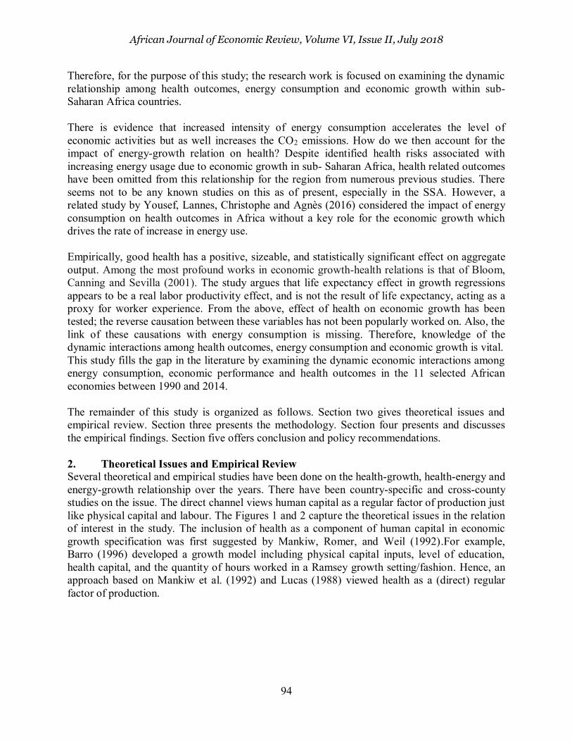
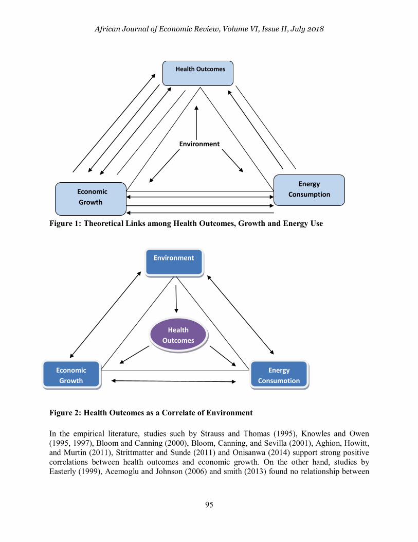
Therefore, for the purpose of this study; the research work is focused on examining the dynamic relationship among health outcomes, energy consumption and economic growth within sub-Saharan Africa countries. There is evidence that increased intensity of energy consumption accelerates the level of economic activities but as well increases the CO2 emissions. How do we then account for the impact of energy-growth relation on health? Despite identified health risks associated with increasing energy usage due to economic growth in sub- Saharan Africa, health related outcomes have been omitted from this relationship for the region from numerous previous studies. There seems not to be any known studies on this as of present, especially in the SSA. However, a related study by Yousef, Lannes, Christophe and Agnès (2016) considered the impact of energy consumption on health outcomes in Africa without a key role for the economic growth which drives the rate of increase in energy use. Empirically, good health has a positive, sizeable, and statistically significant effect on aggregate output. Among the most profound works in economic growth-health relations is that of Bloom, Canning and Sevilla (2001). The study argues that life expectancy effect in growth regressions appears to be a real labor productivity effect, and is not the result of life expectancy, acting as a proxy for worker experience. From the above, effect of health on economic growth has been tested; the reverse causation between these variables has not been popularly worked on. Also, the link of these causations with energy consumption is missing. Therefore, knowledge of the dynamic interactions among health outcomes, energy consumption and economic growth is vital. This study fills the gap in the literature by examining the dynamic economic interactions among energy consumption, economic performance and health outcomes in the 11 selected African economies between 1990 and 2014. The remainder of this study is organized as follows. Section two gives theoretical issues and empirical review. Section three presents the methodology. Section four presents and discusses the empirical findings. Section five offers conclusion and policy recommendations. 2. Theoretical Issues and Empirical Review Several theoretical and empirical studies have been done on the health-growth, health-energy and energy-growth relationship over the years. There have been country-specific and cross-county studies on the issue. The direct channel views human capital as a regular factor of production just like physical capital and labour. The Figures 1 and 2 capture the theoretical issues in the relation of interest in the study. The inclusion of health as a component of human capital in economic growth specification was first suggested by Mankiw, Romer, and Weil (1992).For example, Barro (1996) developed a growth model including physical capital inputs, level of education, health capital, and the quantity of hours worked in a Ramsey growth setting/fashion. Hence, an approach based on Mankiw et al. (1992) and Lucas (1988) viewed health as a (direct) regular factor of production.


95

Figure 1: Theoretical Links among Health Outcomes, Growth and Energy Use

Figure 2: Health Outcomes as a Correlate of Environment

In the empirical literature, studies such by Strauss and Thomas (1995), Knowles and Owen (1995, 1997), Bloom and Canning (2000), Bloom, Canning, and Sevilla (2001), Aghion, Howitt, and Murtin (2011), Strittmatter and Sunde (2011) and Onisanwa (2014) support strong positive correlations between health outcomes and economic growth. On the other hand, studies by Easterly (1999), Acemoglu and Johnson (2006) and smith (2013) found no relationship between

Environment

Health Outcomes

Economic

Growth

Energy

Consumption

Environment

Energy

Consumption

Economic

Growth

Health

Outcomes


96

health outcomes and GDP per capita growth while Frimpong and Adu (2014) found negative effect of population health on economic growth.

Within the framework of health and energy consumption, studies by Smith et al. (2013) and Yousef, Lannes, Christophe, & Agnès, (2016) found Unilateral and bilateral causality for energy consumption and health outcomes relations. The report by UN-DESA report 2004, IEA 2014 and World Energy Outlook report, 2014 noted that Modern energy consumption in Africa is very low and heavily reliant on traditional biomass. This implies that energy might not have had any significant effect on health outcomes in Africa. But studies by Smith (2006), Wang (2009) and Smith et al. (2013) suggested that the relationship between energy consumption on health outcomes may be both positive and negative.

From the above, it is obvious that the health-income growth relationship has been majorly investigated within the framework of economic growth theories as evident in existing studies shown in Table 1. Noting that bi-directional relationship is plausible between the two variables, the reverse effect has been largely understated in various literatures (Barro, 1996). Hence, only a few studies have examined how income growth drives Health outcomes. Even among these studies, there has not been a consensus on both the impact and relative importance of income growths on health outcomes. Three outcomes (within the developed countries) have been found from the literatures which include the positive, negative and neutral effects of income growths on health outcomes.

Table 1: Summary of Related Studies

Author Objective Methodology Findings Stern (1993) Causality between Energy Consumption

and Economic growth Multivariate VAR model EC-GDP

Energy consumption causes economic growth

Asafu-Adjaye (2000) Causality between Energy Consumption and Economic growth

Co-integration and Granger Energy consumption causes economic growth

Ang (2007) Causality between Energy Consumption and Economic growth

Cointegration, VECM Energy consumption causes economic growth

Yu and Choi (1985) Relationship between energy consumption and economic growth

Granger Causality Causality runs from economic growth to energy consumption

Cheng and Lai (1997) The interactions between energy consumption and economic growth

Granger Causality Causality runs from economic growth to energy consumption

Soytas and Sari (2009)

Causality between Energy Consumption and Economic growth

Toda–Yamamoto causality test

No relationship between energy consumption and economic growth

Akinlo (2008) causal relationship between energy consumption and economic growth

Autoregressive distributed lag (ARDL) bounds test

Energy consumption has a significant positive long run impact on economic growth

Yang (2000) re-examined the causality between energy consumption and GDP for Taiwan

Granger causality VECM bi-directional causality between energy consumption and GDP

Knowles and Owen (1995).

effect of incorporating health capital in growth model

Full sample OLS stronger and more robust relationship between income per capita and health capital, than between income per capita and educational human capital


97

Bloom, Canning, and Sevilla (2001)

To investigate the relationship between health and economic growth

two-stage least squares technique

significant relationship between health capital and economic growth

Leung and Wang(2010)

To examine endogenous relationship between health care, life expectancy and output in a neoclassical growth model

Simulation analysis health care directly diverts resources away from goods production, it prolongs life expectancy

Narayan and Mishra (2010)

To investigate the relationship between health and economic growth.

panel cointegration Long run relationship exist between health and economic growth

Frimpong and Adu (2014)

To investigate the relationship between population health and economic growth.

Panel cointegration No relationship exists between health outcomes and GDP per capita growth

Torras (2005) To investigate determinants of health outcomes

two-stage least squares technique

Per-capita income is weak as a determinant of health outcomes

Or (2000) Determinants of health outcomes in OECD Countries

Ordinary least square technique

Health expenditure is more important than income in determining health outcomes

Weil (2014) To examine the relationship between health and economic growth.

Generalized least square technique

There is evidence of bi-directional causality but weak magnitude effect of income on health outcomes

Yousef, Lannes, Christophe, & Agnès, (2016)

To examine causal links between energy consumption and health indicators

Panel Seemingly unrelated regression(SUR) technique

health and energy consumption are strongly linked in Africa.

Wang (2010) To analyze the impacts of energy consumption on environment and public health in China

Exposure-response analysis Energy consumption has both positive and negative effects on health outcomes.

3. Methodology 3.1 Theoretical Framework and Model Specification The theoretical framework employed for this study is the health production function as developed by Or (2000). In the widest sense, a health production function describes the relationship between combinations of medical and non-medical inputs and the resulting output (Smith, 1993). Therefore, health production process depends, in part, on the health-care system and its resource input but also on the non-medical, social, economic and physical conditions. Following this reasoning, general form of a health production function can be specified as: H = f (M, E) (1)

Where H is a measure of the health outcomes, M an indicator of medical resources, and E is a vector of non-medical social, economic and life-style indicators. The theory states that there is positive relationship between health care resources (M) and health outcomes; increasing medical resources implies an improvement in the level and/ or quality of health services supplied to the population. It is also likely that there will be diminishing returns to scale above some level of


98

expenditure. Also, a large number of non-medical, social, economic and physical factors have been suggested as possible determinants of health outcomes by different epidemiological, demographic and economic studies (Barro, 1996; Smith, 2003 and Torras, 2005). Or (2000) classified the non-medical factors into three major categories to simplify the discussion. These are physical environment, life styles and socio-economic factors.

The impact of factors relating to the physical environment such as water and soil quality, as well as noise and air pollution on health will be different. For example, it is expected that the effect of quality water and soil will be positive while that of noise and air pollution will be negative. According to Or (2000), there is a growing awareness about the strong relationship between health and life styles. In the most general sense, “life style” refers to all factors over which individuals have some control, such as alcohol consumption, exercise, personal hygiene, etc.

Furthermore, the theory specified three factors which determine the socio-economic environment both for individuals and for society. These are income, education and work. There is a positive relationship between income level and health. Higher income results in higher consumption of goods that have a direct impact on the quality of life such as food, housing, schooling, etc. The distribution of income in a country has also been suggested as an important factor determining health status (Preston, 1975; Wilkinson, 1992; Winegarden, 1978, 1984; Saunders, 1996; Kawachi and Kennedy, 1997). Several explanations have been given for the way education influences health. Education seems to determine many of the decisions which affect the quality of life: choice of job, ability to select a healthy diet and avoid unhealthy habits, efficient use of medical care, etc. Occupation is also suggested as an important intervening variable in this relationship (Leigh, 1983; Kemna, 1987).

With reference to the health production function, the model for this study is therefore specified as follows:

itititiit EMH (2)

This model is specified following model specification by Or (2000). In this model, H is health outcome measured by life expectancy, M is a vector of medical variables measured by health care expenditure, E is a vector of non-medical factors generally referred to as environmental factors by Or (2000) which are restricted to energy consumption, income and education for the purpose of this study following Torras, (2005). The subscripts i and t refer to country and time respectively. 𝛽 and 𝛾 are vectors of the coefficients on M and E, respectively. Also, 𝛽 > 0 and 𝛾 can be positive or negative depending on the variable. The constant terms,𝛼, control for country characteristics which are presumed to be stable over the period studied.

In a more specific sense, taking inference from the model specification above through the health production function, we can therefore clearly state the relationship between the various variables of interest. Theory has also identified health care expenditure and education as additional factors which may affect the health outcomes:

ititiitiitiitiiit vEXSYEH 43210 (3)


99

Where H, E, Y, S and EX are health outcomes, energy consumption, national income, education and health care expenditure respectively. For 𝛽 > 0 shows that we expect all the identified independent variables to have positive effect on health outcomes.

However, due to the dynamic nature inherent in this relationship, a panel vector autoregressive (PVAR) framework is employed to examine the effects of energy consumption and economic growth on health outcomes using the impulse response analysis, forecast error variance decomposition as well as causality analysis only. The PVAR version of equation (3) is thus:

m

j

m

j

m

j

hit

n

mjit

ixjtijtjtijtjtijit

hiit XYEHH

1 1 1

1

0,,3,,2,, (4)

m

j

m

J

m

j

yit

n

mjit

ixjtijtjtijtjtijit

yiit XHEYY

1 1 1

1

0,,3,,2,, (5)

m

j

m

j

m

j

eit

n

mjit

ixjtijtjtijtjtijit

eiit XHYEE

1 1 1

1

0,,3,,2,, (6)

Where jitX the (k x 1) is a vector of control variables for 𝛾,𝛼 and 𝛽 are the parameters for the model. The PVAR approach inherits advantages over the traditional VAR model is that the variables in the system are treated as endogenous (or weakly exogenous in some cases) (see Sims, 1980). The PVAR procedure also has advantages based on a panel-data framework that allows for unobserved individual heterogeneity for all the variables by introducing fixed effects, which enhances the consistency of the estimation. The dynamic nature of energy consumption, economic growth and health outcomes means we cannot be restricted to only a single equation with one variable designated as the dependent variable, explained by other variables that are assumed to be weakly exogenous for the parameters of interest. However, there are criticisms to the estimation of VAR models as they are a-theoretic since they are not based on any prior economic theory. This makes it difficult to interpret the coefficients obtained but being employed to make further analyses such as impulse responses.

3.2 Estimation Techniques

This study utilizes the panel data method of analysis. The main usefulness of the approach lies in its ability to allow for differences in the aggregate health production functions across economies. The use of panel techniques enables the power of the tests to be increased and makes it possible to include heterogeneity between countries. Panel data provides a larger number of point data, allows higher degrees of freedom and reduces the collinearity between the regressors. The panel unit root tests, panel cointegration as well as the impulse response, panel Granger non-causality and forecast error variance decomposition analyses via least square estimator of equations (4) to (6) are specifically explored to achieve the aim of the study. The panel data unit root tests statistics asymptotically follow a normal distribution instead of nonconventional distributions. A number of such tests have appeared in the literature. Recent developments in the panel unit root tests include Levin, Lin and Chu ((LLC, 2002), Im, peseran and Shin (IPS, 2003), Maddala and Wu (1999), Choi (2001) and Hadri (2000). From among different panel unit root tests developed in the literature, LLC and IPS are the most popular. Both of the tests are based on the ADF principle. However, LLC assumes homogeneity in the dynamics of the autoregressive


100

coefficients for all panel members. In contrast, the IPS is more general in the sense that it allows for heterogeneity in these dynamics. Therefore, it is described as a ‘‘heterogeneous panel unit

root test’’. It is particularly reasonable to allow for such heterogeneity in choosing the lag length in ADF tests when imposing uniform lag length is not appropriate. In addition, slope heterogeneity is more reasonable in the case where cross-country data are used. In this case, heterogeneity arises because of differences in economic conditions and degree of development in each country. As a result, the test developers have shown that this test has higher power than other tests in its class, including LLC. The IPS unit root test is used in this study to test for stationarity of the panel data because it allows for heterogeneity in studying the dynamics among energy consumption, economic growth and health outcomes, as such can easily be adaptable for data obtained for the selected SSA countries.

Panel cointegration tests examine the long-run relationships amongst variables of interest. The study applied the Pedronic and Kao residual cointegration tests because they are based on Engle-Granger (1987) two-step (residual-based) cointegration tests which allows for heterogeneous intercepts and trend coefficients across cross-sections. Also, they yield more efficient results where the time series is larger than the number of cross-sections (i.e. N < T). 275 observations were included in the test. Outcomes of each variable of interest as independent variable are considered under Pedronic test with relevant Statistics and probability values, while for Kao test, one outcome is considered (i.e. one p-value). The null hypothesis states that there is no cointegration while the alternative specifies there is cointegration. If the p-value is greater than 5%, we cannot reject null hypothesis. The decision rule is that if the majority is not significant, we cannot reject null hypothesis, meaning that the variable are not cointegrated, i.e. there is no long-run relationship.

Apart from the dynamic aspect of the relationship among the variables, a test of panel causality is done using Holtz-Eakin et al. (1988):

∆𝑌𝑖𝑡 = ∑ 𝛼𝑗∆𝑌𝑖𝑡−𝑗𝑚𝑗=1 + ∑ 𝛿𝑗

𝑚𝑗=1 ∆𝑋𝑖𝑡−𝑗 + ∆𝑢𝑖𝑡 , (7)

∆𝑋𝑖𝑡 = ∑ 𝛽𝑗𝑚𝑗=1 ∆𝑌𝑖𝑡−𝑗 + ∑ 𝛾𝑗

𝑚𝑗=1 ∆𝑋𝑖𝑡−𝑗 + ∆𝑣𝑖𝑡,

Where 𝑌𝑖𝑡 and 𝑋𝑖𝑡 are the two cointegrated variables, 𝑖 = 1, … , 𝑁 represents cross-sectional panel members, and 𝑢 𝑖𝑡and 𝑣𝑖𝑡 are error terms. This model differs from the standard causality model in that it adds two terms, 𝑓 𝑥𝑖and 𝑓𝑦𝑖 which are individual fixed effects for the panel member i. In the equations above, the lagged dependent variables are correlated with the error terms, including the fixed effects. The differencing introduces a simultaneity problem because lagged endogenous variables on the right-hand side are correlated with the new differenced error term. In addition, heteroscedasticity is expected to be present because in the panel data heterogeneous errors might exist with different panel members. To deal with these problems, an instrumental variable procedure is traditionally used in estimating the model, which produces consistent estimates of the parameters. Assuming that 𝑢𝑖𝑡 and 𝑣 𝑖𝑡 are serially uncorrelated, the second or more lagged values of 𝑌𝑖𝑡 and 𝑋𝑖𝑡 may be used as instruments in the instrumental variable estimation (Easterly et al., 1997). Then, to test for the causality, the joint hypotheses 𝛿𝑗 = 0 for 𝑗 = 1, . . . , 𝑚 and 𝛽𝑗 = 0 for 𝑗 = 1, . . . , 𝑚 is simply tested. The test statistics follow a chi-squared distribution with (k–m) degrees of freedom. The variable X is said not to Granger-


101

cause the variable Y if all the coefficients of lagged X in Equation (7) are not significantly different from zero, because it implies that the history of X does not improve the prediction of Y.

3.3 Data: Definition, Measurement and Sources

The data employed in analyzing the dynamic relationship between energy consumption, economic growth and health outcomes in sub-Saharan African countries (Benin, Cameroon, Cote d’Ivoire, Gabon, Ghana, Kenya, Nigeria, Senegal, South Africa, Togo and Zimbabwe. Each region of the sub-Sahara Africa is well represented) between 1990 and 2014 is secondary. The study utilizes data for real GDP per capita, energy consumption and life expectancy. In this study, energy consumption is expressed in kilogram of oil equivalents (kgoe). We obtained the real GDP per capita series by deflating the nominal figure by the GDP deflator (2000 as the base year). Nominal GDP per capita, Life expectancy at birth and energy consumption data for countries observed is obtained from the World Bank data base through World Bank development indicators Data 2016. Life expectancy at birth is used as a measure of health outcomes because it is the most common health outcome indicator containing all information about health impacts (Yousef et.al, 2016). Improvements in health are translated in additional years of living. Hence, it has been considered the most reliable, particularly when performing international studies (Leu, 1986; Hitiris and Postnet, 1992). GDP per capita is used as a proxy for National Income. This is because it is the most appropriate standard of comparison among different countries. For energy consumption, we use energy consumption per kg of oil equivalent. This is because energy consumption is an indicator of energy supply. It varies from a country to another mainly because the productive sector varies and its consumption varies. The choice of control variables follows Or (2000). Health care expenditure is a representative of medical factors, CO2 and population growth represents environmental factors while education represents the social status.

4. Results 4.1 Panel Unit Root and Cointegration Tests14 Panel Unit Root The variables of interest are a mixture of I(1). The study applied the Pedronic and Kao residual cointegration tests because they are based on Engle-Granger (1987) two-step cointegration tests which allows for heterogeneous intercepts and trend coefficients across cross-sections. Also, they yield more efficient results where the time series is larger than the number of cross-sections (i.e. N < T). The cointegration tests results for each independent variables of interest showed that under the Pedroni test, the Primary school enrolments was significant under Panel ADF statistics with p-value of 0.0119 less than 5%. However, it is noticed that majority of statistics of the other independent variables are not significant because their p-values greater than 5%; as such we cannot reject the null hypothesis, meaning that the variables are not cointegrated. The same results were obtained under Kao residual cointegration test. To this effect, the empirical properties of the variables examined require estimation of the VAR in first differences, since no cointegration relationships exist between the (non stationary) variables (in level).

14Results are available upon request. Omitted to save space.


102

4.2 Panel Vector Autoregressive Estimates The dynamic effect and the degree of importance of change in energy consumption (LNGY) and income on health outcomes using historical data of eleven sub-Sahara African countries is discussed in what follows. The impulse response functions (IRFs) is used to show the effect while the panel error variance decomposition (VDC) shows the relative importance of these variables in explaining the behaviour of each other. The correct lag length selection is essential for panel VAR, and lag 3 is found to be optimal using Schwarz information criterion (SC) Table 4.1.1 Unit Root Tests for the Variables at Levels

Im, Pesaran and Shin W-stat ADF - Fisher Chi-square

Variables Cross

Section Obs Statistics Probability Statistics Probability CO2 11 242 -0.57988 0.2810 26.5508 0.2288 LNGY 11 242 1.64193 0.9497 10.0620 0.9857 LPRY 11 160 2.98784 0.9986 7.25004 0.9958 LGDP 11 253 2.94255 0.9984 12.1874 0.9534 LHLTH 11 193 3.40447 0.9997 4.35576 1.0000 LLIFE 11 253 -24.2352 0.0000 474.953 0.0000

Table 4.1.2 Unit Root Tests for the Variables at First Difference

Im, Pesaran and Shin W-stat ADF - Fisher Chi-square

Variables Cross

Section Obs Statistics Probability Statistics Probability D(CO2) 11 231 -8.13845 0.0000 105.201 0.0000 D(LNGY) 11 231 -7.65072 0.0000 99.4703 0.0000 D(LPRY) 11 139 -2.38771 0.0085 39.3919 0.0060 D(LGDP) 11 242 -3.86543 0.0001 50.5939 0.0005 D(LHLTH) 11 182 -3.1369 0.0009 43.2259 0.0044


103

Table 4.1.3 Unit Root Tests for the Variables (Order of Integration)

Variables Im, Pesaran and Shin W-stat ADF - Fisher Chi-square CO2 I(1) I(1) LNGY I(1) I(1) LPRY I(1) I(1) LGDP I(1) I(1) LHLTH I(1) I(1) LLIFE I(0), I(1) I(0), I(1)

Table 4.2 Pedronic Residual Cointegration Test

Trend assumption: Deterministic intercept and trend

Independent variable Panel v-Statistic

Panel rho-Statistic

Panel PP-Statistic

Panel ADF-Statistic

LLIFE -2.845169 4.079533 2.460161 2.774417 [ 0.9978] [ 1.0000] [ 0.9931] [ 0.9972]

LGDP -1.61459 4.055733 -0.570296 -1.460862 [ 0.9468] [ 1.0000] [ 0.2842] [ 0.0720]

POP -1.56885 4.502784 2.232944 2.273851 [ 0.9417] [ 1.0000] [ 0.9872] [ 0.9885]

LHLT -1.666186 3.306843 -0.143933 -1.511111 [ 0.9522] [ 0.9995] [ 0.4428] [ 0.0654]

LPRY -0.071711 3.902797 -5.442831 -2.261113 [ 0.5286] [ 1.0000] [ 0.0000] [ 0.0119]

LENERGY -2.068311 4.081828 -1.035601 0.020356 [ 0.9807] [ 1.0000] [ 0.1502] [ 0.5081]

CO2 -4.039437 2.521018 -29.38254 -10.5027 [ 1.0000] [ 0.9941] [ 0.0000] [ 0.0000]

4.3 The Impulse Response Function (IRF)

The impulse response functions (IRF) traces the temporal and directional response of an endogenous variable to a change in one of the structural innovations within a model. The significance of response is measured by the relative position of the response line (Solid line) to the zero line. The farther away the solid line from the zero line, the more significant the response. A solid line close to the zero line implies that response of a variable is not significant or substantial to a shock to the other variables. With regard to this study, of particular interest is the dynamic interaction among energy consumption, economic growth and health outcomes in


104

the selected countries. Table 4.3.1 to 4.3.2 show the impulse responses of the variables. From Table 4.3.1, life expectancy does not respond to shock to any of the variables in the first period except a positive shock to itself in the first period and continues to increase till period 6, then, decreases slightly from 0.00052% in period 7 to 0.0003% in year 10.

This result reveals the nature of life expectancy where it does not respond instantaneously to shock to other variables. This means that the nature of relationship between health outcomes and other variables is a lagged one and not contemporaneous. As such, improvement in provision of medical facilities and increase in income may not lead to immediate improvement in the health of people. This is reasonable as the effect of income for example will first apply to factors such as good nutrition and quality hygiene practice before it translates to good health outcomes.

Also, the response of life expectancy to health care expenditure per capita began slightly in the second period from the lowest 0.000008% and increases overtime to 0.000229% in year 8, then declines in period 9 and settles at 0.00018% in period 10. Similarly, the impulse to output generates a very negligible response from life LLIFE all through the periods. As such, figure 4.6c shows that a shock to GDP per capita leaves Life expectancy (LLIFE), to a larger extent, unaffected. Moreover, Column 6 Table 4.3.1, LLIFE responds positively to energy consumption (LNGY) but this response is non-substantial.

Table 4.3.1 Response of D(LLIFE): Period D(LLIFE) D(LHLTH) D(LGDP) D(CO2) D(LNGY) POP D(PRY)

1 7.61E-05 0.000000 0.000000 0.000000 0.000000 0.000000 0.000000 2 0.000190 8.33E-06 6.35E-06 2.85E-06 1.47E-05 -2.30E-06 -5.15E-06 3 0.000308 4.57E-05 1.89E-05 3.12E-05 4.87E-05 -1.07E-05 -2.21E-05 4 0.000416 0.000102 2.86E-05 5.31E-05 7.44E-05 -2.29E-05 -4.20E-05 5 0.000495 0.000154 3.52E-05 6.65E-05 8.81E-05 -4.36E-05 -6.63E-05 6 0.000532 0.000197 3.27E-05 7.85E-05 8.43E-05 -6.07E-05 -9.15E-05 7 0.000527 0.000223 2.10E-05 8.96E-05 6.61E-05 -7.10E-05 -0.00011 8 0.000481 0.000229 3.83E-06 9.49E-05 4.30E-05 -7.19E-05 -0.00012 9 0.000403 0.000214 -1.53E-05 9.39E-05 1.61E-05 -6.35E-05 -0.00012 10 0.000305 0.000184 -3.22E-05 8.76E-05 -9.76E-06 -4.47E-05 -0.00012

Source: Author’s Computation

In Table 4.3.1, column 5 reveals that there is positive but non-substantial response of Life expectancy to impulse Carbon emission. This shows that health outcomes measure in the sub-Sahara Africa may not have been impacted greatly by the quality of the environment. This may be informed by the cushioning effect of foreign aids such as periodic supply of vaccines, technical support, and other disease control measures put in place by donor countries and international organizations. LLIFE responds negatively but insignificant to Population (POP) and Primary school enrolment (PRY). In reference to the above, the negligible effect of poor environmental quality on health outcome can be adduced to low level of industrial activities in the SSA which generates lower level of carbon emission. This means that carbon emission is not among the main factors that affect the health of people in SSA. The low industrial development of SSA has not made carbon emission so great an issue to consider in the health outcomes of the region. In the same vein, though health outcomes responded negatively to population growth and


105

the literacy level, yet the real effect on health outcomes in SSA in small. According to Education For All Global Monitoring Report (EFAGMR, 2010), the deficit of number of children out of school is still very high and represents 45% of the global out-of-school population. If the quality and content of education given in SSA does not involve the one for improving personal hygiene and health care, progress made in primary school enrolment as recorded by EFAGMR (2010) in the region may not be substantial enough to make real impact on health outcomes in the region.

The response was not substantial and falling throughout with period 1 to 6 being positive while the response became negative in period 7 to 10. This implies that good health outcomes can spur economic growth but a point may be reached where propensity of people to live healthier and longer will not have as much impact as one would expect on the economic growth. Good health will tend to impact positively on the workforce. This position is well supported by Bloom, Canning, and Sevilla (2001) and Narayan, Narayan and Mishra (2010).

Figure 4.3.1: Response of Energy Consumption to change in Life expectancy The nature and response of the LGDP to LLIFE represents diminishing returns to good health. This means good health and propensity to live longer can not in itself sustain income growth indefinitely in the SSA. This may be due to increase in the number of dependants among the active population. As people live longer, the demographic distribution of the population will change as there would be increase in the number of people reaching old age. For example, payment of pension benefits to retirees may tend to increase which may divert resources from investing or productive activities.


106

Table 4.3.2 Response of D(LGDP): Period D(LLIFE) D(LHLTH) D(LGDP) D(CO2) D(LNGY) POP D(PRY)

1 0.000414 0.002034 0.008114 0.000000 0.000000 0.000000 0.000000 2 0.001326 0.002253 0.002752 -0.00083 -0.00178 0.000305 0.000602 3 0.000880 0.001533 0.002230 3.34E-05 -0.00114 -0.00034 -4.32E-06 4 0.000613 0.000856 0.000888 -3.29E-05 -0.00078 -0.00019 0.000107 5 0.000359 -5.14E-05 0.000310 0.000177 -0.00113 -0.00058 0.000172 6 2.73E-05 -0.00038 -4.58E-05 -4.91E-05 -0.00048 -0.00044 -3.99E-05 7 -0.00015 -0.00038 -0.00031 -9.21E-05 -0.00027 -0.00059 -1.71E-05 8 -0.00023 -0.00021 -0.00039 -1.24E-05 -0.00011 -0.00044 0.000122 9 -0.00019 -0.00016 -0.00038 -5.36E-05 1.08E-06 -0.0004 0.000123 10 -8.51E-05 -0.0001 -0.00028 -3.27E-05 -1.62E-05 -0.00033 0.000153

Source: Author’s Computation

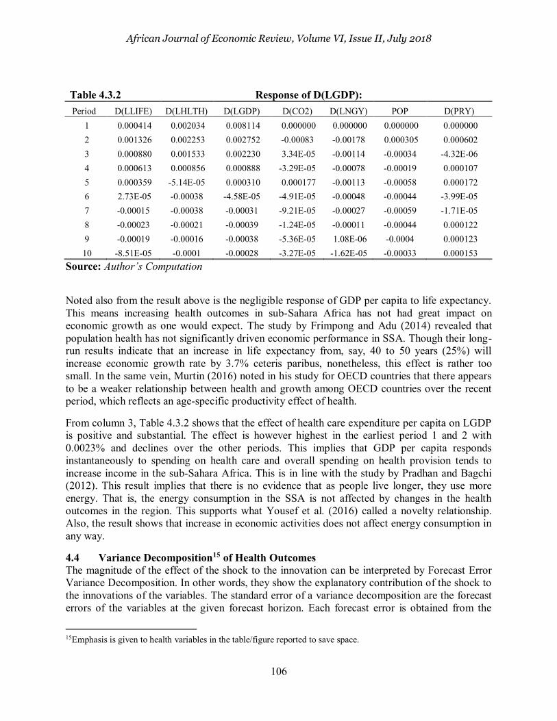
Noted also from the result above is the negligible response of GDP per capita to life expectancy. This means increasing health outcomes in sub-Sahara Africa has not had great impact on economic growth as one would expect. The study by Frimpong and Adu (2014) revealed that population health has not significantly driven economic performance in SSA. Though their long-run results indicate that an increase in life expectancy from, say, 40 to 50 years (25%) will increase economic growth rate by 3.7% ceteris paribus, nonetheless, this effect is rather too small. In the same vein, Murtin (2016) noted in his study for OECD countries that there appears to be a weaker relationship between health and growth among OECD countries over the recent period, which reflects an age-specific productivity effect of health.

From column 3, Table 4.3.2 shows that the effect of health care expenditure per capita on LGDP is positive and substantial. The effect is however highest in the earliest period 1 and 2 with 0.0023% and declines over the other periods. This implies that GDP per capita responds instantaneously to spending on health care and overall spending on health provision tends to increase income in the sub-Sahara Africa. This is in line with the study by Pradhan and Bagchi (2012). This result implies that there is no evidence that as people live longer, they use more energy. That is, the energy consumption in the SSA is not affected by changes in the health outcomes in the region. This supports what Yousef et al. (2016) called a novelty relationship. Also, the result shows that increase in economic activities does not affect energy consumption in any way.

4.4 Variance Decomposition15 of Health Outcomes The magnitude of the effect of the shock to the innovation can be interpreted by Forecast Error Variance Decomposition. In other words, they show the explanatory contribution of the shock to the innovations of the variables. The standard error of a variance decomposition are the forecast errors of the variables at the given forecast horizon. Each forecast error is obtained from the

15Emphasis is given to health variables in the table/figure reported to save space.


107

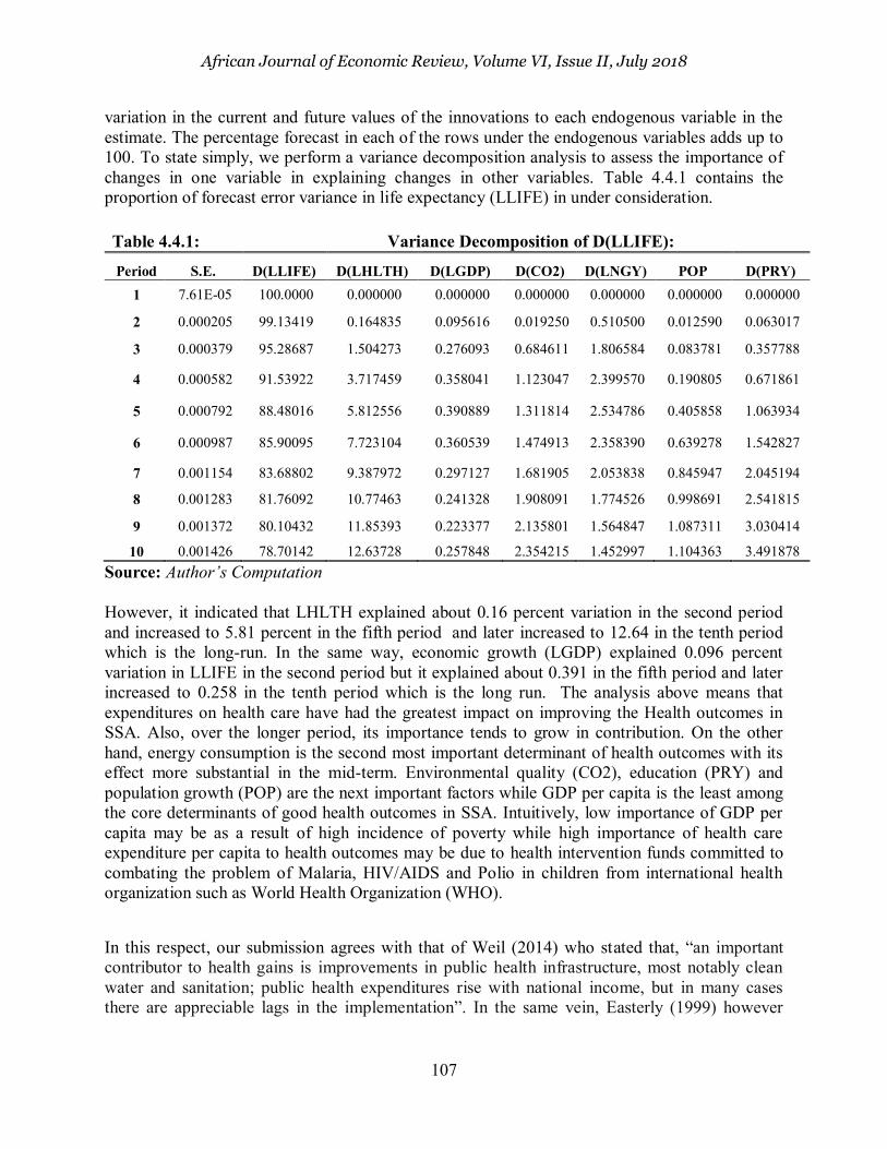
variation in the current and future values of the innovations to each endogenous variable in the estimate. The percentage forecast in each of the rows under the endogenous variables adds up to 100. To state simply, we perform a variance decomposition analysis to assess the importance of changes in one variable in explaining changes in other variables. Table 4.4.1 contains the proportion of forecast error variance in life expectancy (LLIFE) in under consideration.

Table 4.4.1: Variance Decomposition of D(LLIFE):

Period S.E. D(LLIFE) D(LHLTH) D(LGDP) D(CO2) D(LNGY) POP D(PRY) 1 7.61E-05 100.0000 0.000000 0.000000 0.000000 0.000000 0.000000 0.000000

2 0.000205 99.13419 0.164835 0.095616 0.019250 0.510500 0.012590 0.063017

3 0.000379 95.28687 1.504273 0.276093 0.684611 1.806584 0.083781 0.357788

4 0.000582 91.53922 3.717459 0.358041 1.123047 2.399570 0.190805 0.671861

5 0.000792 88.48016 5.812556 0.390889 1.311814 2.534786 0.405858 1.063934

6 0.000987 85.90095 7.723104 0.360539 1.474913 2.358390 0.639278 1.542827

7 0.001154 83.68802 9.387972 0.297127 1.681905 2.053838 0.845947 2.045194

8 0.001283 81.76092 10.77463 0.241328 1.908091 1.774526 0.998691 2.541815

9 0.001372 80.10432 11.85393 0.223377 2.135801 1.564847 1.087311 3.030414

10 0.001426 78.70142 12.63728 0.257848 2.354215 1.452997 1.104363 3.491878 Source: Author’s Computation However, it indicated that LHLTH explained about 0.16 percent variation in the second period and increased to 5.81 percent in the fifth period and later increased to 12.64 in the tenth period which is the long-run. In the same way, economic growth (LGDP) explained 0.096 percent variation in LLIFE in the second period but it explained about 0.391 in the fifth period and later increased to 0.258 in the tenth period which is the long run. The analysis above means that expenditures on health care have had the greatest impact on improving the Health outcomes in SSA. Also, over the longer period, its importance tends to grow in contribution. On the other hand, energy consumption is the second most important determinant of health outcomes with its effect more substantial in the mid-term. Environmental quality (CO2), education (PRY) and population growth (POP) are the next important factors while GDP per capita is the least among the core determinants of good health outcomes in SSA. Intuitively, low importance of GDP per capita may be as a result of high incidence of poverty while high importance of health care expenditure per capita to health outcomes may be due to health intervention funds committed to combating the problem of Malaria, HIV/AIDS and Polio in children from international health organization such as World Health Organization (WHO).

In this respect, our submission agrees with that of Weil (2014) who stated that, “an important contributor to health gains is improvements in public health infrastructure, most notably clean water and sanitation; public health expenditures rise with national income, but in many cases there are appreciable lags in the implementation”. In the same vein, Easterly (1999) however


108

noted that the low contribution of income growth to health outcomes could be adduced to “long

and variable lags” in the translation of higher income growth into better health.

The important determinants of energy consumption are the environmental quality, health care expenditure, life expectancy and economic growth. The most important among them is the quality of the environment as measured by CO2 emission. Increasing Industrial activities means increase need for sanitation and protection of the environment. These activities generate wastes which are released into the environment. The importance of economic growth to energy consumption can be intuitively inferred from increasing economic and industrial activities which demand more energy in SSA. Noting the importance of Health care expenditure per capita to our variables of interest will make us examine the reverse contributions of other variables to it. Table 4.4.2 below shows the proportion of forecast error variance in health expenditure per capita performance in sub-Sahara African Countries as explained by the changes to innovations of the considered endogenous variables. No short-run effect is observed from variables LGDP, CO2, LNGY, POP and PRY because their contribution is zero percent in period one. But life expectancy (LLIFE) will affect changes in Health expenditures in the short-run because changes to LLIFE will explain 0.5% variations in the LHLTH in period 1. This declines to 0.47% in the third period while it increases to 0.57% in period four but continue to increase to 0.72% in period 10. On the other hand, from period 2 the effect of LGDP increase from approximately 0.3% to 0.81% in period 10. The other endogenous variables have the same increasing effect on LHLTH from period 2 all through period 10. However, Energy consumption (LNGY) has the highest magnitude effect from 10.98% in period 2 to 17.55% in period 10.

Table 4.4.2 Variance Decomposition of D(LHLTH): Period S.E. D(LLIFE) D(LHLTH) D(LGDP) D(CO2) D(LNGY) POP D(PRY)

1 0.054584 0.584791 99.41521 0.000000 0.000000 0.000000 0.000000 0.000000

2 0.060212 0.487502 86.99926 0.029634 0.002038 10.97795 1.493179 0.010439

3 0.061247 0.477702 84.92904 0.641137 0.013628 11.84440 1.460301 0.633787

4 0.064383 0.570161 79.13672 0.652678 0.412708 17.23289 1.392060 0.602790

5 0.064722 0.606104 79.13581 0.645862 0.431053 17.12536 1.408132 0.647681

6 0.064990 0.629418 78.48520 0.735159 0.478326 17.58390 1.443030 0.644967

7 0.065082 0.666074 78.37755 0.804579 0.515590 17.53740 1.445188 0.653620

8 0.065125 0.695575 78.32591 0.809316 0.515937 17.55005 1.449248 0.653963

9 0.065147 0.717738 78.31517 0.808781 0.516429 17.53980 1.448321 0.653765

10 0.065173 0.725000 78.27464 0.808609 0.524972 17.55244 1.458843 0.655492 Source: Author’s Computation From the above, energy consumption is the most critical factor among others in explaining variations in health care expenditure per capita with the effect increasing over the years in SSA. This means areas with easy access to clean source of energy will command and attract greater health expenditure. We may look at this from the point of cost efficiency. Thereby, it may be more cost effective to set up a medical facility in areas with abundant power supply than areas


109

with less supply in SSA. Since availability of energy source in the short and long run reduces expenditure in setting up medical centre, it is only rational that medical expenditures will trail the time of availability of energy. This may be the reason for high concentration of sophisticated medical centers in urban areas than the rural areas. The change in Health care expenditure per capita is more important in explaining Health outcomes than economic growth or energy consumption in SSA. Similarly, the most important factor in determining Economic growth is the rate of spending on health care and not necessarily Life expectancy or energy consumption even though they are important as well. A change in Carbon emission will have the highest impact on Energy consumption. This means energy consumption will change as there is demand for more quality environment. The reverse however is not the case as energy consumption has greater impacts on how much is spent on health care.

4.5 Test of Causality In this section, causality among Energy consumption, Economic growth and Health outcomes in the selected SSA Countries was investigated using Panel VAR Granger Causality/Block Exogeneity Wald test. The Table 4.5.1 below presents the result of the Granger Causality/Block Exogeneity Wald test based on the Panel series being examined. The decision rule specifies that there is presence of Causality where and if p < 0.05.

From Table 4.5.1 column 1, we found no evidence of causality running from life expectancy to energy consumption or economic growth at 5% level of significance. In column 4 and 6 also, there is no evidence of causality running from either energy consumption or economic growth to life expectancy. This is because their p-value is greater than 0.05. This implies that neither economic growth nor energy consumption have any impact on health outcomes in sub-Sahara Africa. Also, improvements in health outcomes cannot improve significantly the level of economic growth. This outcome is in line with findings by Torras (2005) which casts doubt on the importance of per-capita income in explaining environmental and health outcomes. However, this result is in contrast with the evidence provided by Yousef et al. (2016) who found strong causal link between energy consumption and health outcomes in Africa. Nonetheless, there is an evidence of causality running from energy consumption to life expectancy if we consider 10% level of significance with a p-value of 0.0614 in column 6. This means at 10%, health outocmes will be greatly improved with every increase in energy consumption which would have corroborate the findings of Yousef et al. (2016).

The reason for absence of any meaningful link between life expectancy and economic growth could be adduced to the long lags between income and health. As noted by Pritchett and Summers (1996); Easterly (1999) that the elements of Health outcomes does not respond instanteneously to increase in income. Usually, change in health outcomes requires consistent growth in income over a long period of time. Here the permanent income hypothesis is applicable. A poor individual will not change its consumption style to a more nourishing one if he does not perceive its change in income as a permanent one. The consistent economic growth experienced in the sub-Sahara Africa is still currently below two decades with slow growth in between.


110

* Significant at 1%; ** Significant at 5%; *** Significant at 10%

TABLE 4.5.1 Causal Relationship Test among Energy Consumption, Economic Growth and Health Outcomes

Dependent Variable D(LLIFE) D(LHLTH) D(LGDP) D(CO2) D(LENERGY) POP D(PRY) All

D(LLIFE) 0 2.217083 4.622934 13.689 7.353472 2.270526 2.053885 41.54377*

(0.5286) (0.2016) (0.0034*) (0.0614***) (0.5182) (0.5613) (0.0013)

D(LHLTH) 2.209414 0 0.5223 2.3833 14.64364 3.922704 1.748444 25.28645

(0.5301) (0.9140) (0.4968) (0.0021*) (0.2699) (0.6262) (0.1172)

D(LGDP) 2.918807 3.181547

0

0.558492 2.858183 2.146966 0.404580 10.70386

(0.4043) (0.3645) (0.9059) (0.4140) (0.5425) (0.9393) (0.9065)

D(CO2) 12.09248 1.218211 7.548038

0

2.603660 16.23207 2.802955 61.01408

(0.0071*) (0.7486) (0.0563***) (0.4568) (0.0010*) (0.4230) (0.0000*)

D(LENERGY) 1.865306 3.612560 2.398611 2.277229 0 0.771174 1.736775 11.87676

(0.6008) (0.3065) (0.4939) (0.5169) (0.8563) (0.6288) (0.8535)

POP 8.157170 10.24954 4.197427 1.518465 1.863572 0 2.197961 23.40465

(0.0429**) (0.0166**) (0.2409) (0.6780) (0.6012) (0.5324) (0.1755)

D(PRY) 1.759338 0.814859 2.087851 0.681015 3.371375 6.013181 0 17.78007

(0.6238) (0.8459) (0.5544) (0.8777) (0.3378) (0.1110) (0.4702)


111

4.6 Model Stability Test: The result of the stability test using the roots characteristics of polynomial is as shown in the Figure 4.6.1. From the test result conducted, it could be clearly seen from the Figure that no roots lay outside the unit circle; hence, it can be concluded that the model is stable. Thus, the impact of the shocks dies out. It means the coefficient estimates are reliable and can thus be employed for predictive purposes.

-1.5

-1.0

-0.5

0.0

0.5

1.0

1.5

-1.5 -1.0 -0.5 0.0 0.5 1.0 1.5

Inverse Roots of AR Characteristic Polynomial

Figure 4.6.1: Stability Test

5. Conclusions and Policy Recommendations.

The study investigated the relationship between energy consumption, economic growth and health outcomes using selected Sub-Saharan Africa countries. The study revealed that neither economic growth nor energy consumption was found to affect health outcomes significantly in the region. The study however shows that medical factor such as health care expenditure remains an important determinant of health outcomes in SSA. Economic diversification towards industrialization should be made a top priority with the aim of minimizing the effect of global commodity price shock on sub-Saharan African economy and to establish a steady but predictable growth. Also, the internal health policy should be designed to reflect the global health policies from international organisation such as IMF. The health policy goals in the SSA must be clearly defined in a measurable way and strategic efforts towards achieving the goals should be stated and commenced without delay when the economy of the SSA is plagued with problems of slow economic growth. Any policy to improve life expectancy should also include


112

the development of human capital and how this capital can be put into efficient use. Public awareness and enlightenment on the need for environmental preservation and the consequences of environmental pollution should be ensured.

Also, the causal link between life expectancy to energy consumption or economic growth was investigated in the study. We found no evidence of causality running from life expectancy to energy consumption or economic growth at 5% level of significance. In column 4 and 6 also, there is no evidence of causality running from either energy consumption or economic growth to life expectancy. This is because their p-value is greater than 0.05. This implies that neither economic growth nor energy consumption have any causal relation on health outcomes in sub-Sahara Africa. Also, improvements in health outcomes cannot improve significantly the level of economic growth. This outcome is in line with findings by Torras (2005) which casts doubt on the importance of per-capita income in explaining environmental and health outcomes. However, this result is in contrast with the evidence provided by Yousef et al. (2016) who found strong causal link between energy consumption and health outcomes in Africa. Nonetheless, there is an evidence of causality running from energy consumption to life expectancy if we consider 10% level of significance with a p-value of 0.0614 in column 6. This means at 10%, health outocmes will be greatly improved with every increase in energy consumption which would have corroborate the findings of Yousef et al. (2016).

Access to modern energy should be made affordable to all through the provision of subsidy especially for the poor. Other sources of renewable energy apart from hydro electricity should be developed. Since report from International Energy Agency (IEA) says that the solar energy in Africa alone can generate electricity for about three continents.

References

Akinlo, A. E. (2008). “Energy consumption and economic growth: evidence from 11 Sub-Sahara African countries”. Energy Economics, 30 (5), pp. 2391–2400. Akinlo, A.E. (2009). “Electricity consumption and economic growth in Nigeria: Evidence from

cointegration and co-feature analysis”, Journal of Policy Modeling, 31, pp. 681-693. Altinay, G., Karagol, E., (2005). Electricity consumption and economic growth: evidence for Turkey. Energy Economics 27, 849–856. Ang, J. B. (2007). “CO2 emissions, energy consumption, and output in France”, Energy Policy, 35(10), pp. 4772-4778. Barro, R. (1996). Three models of health and economic growth. Unpublished manuscript. Cambridge, MA: Harvard University. Bloom, D. E., & Canning, D. (2000). The health and wealth of nations. Science, 287, 1207–

1208.

Bloom, D. E., Canning, D., & Sevilla, J. (2001). The effect of health on economic growth: Theory and evidence. NBER Working Paper No. 8587.


113

Chang, B.S., (1997). Energy consumption and economic growth in Brazil, Mexico and Venezuela: a time series analysis. Applied Economics Letters 4 (11), 671–674. Chang, B.S., Lai, T.W. (1997). An investigation of co-integration and causality between energy consumption and economic activity in Taiwan. Energy Economics, 19, 435–444. Cutler,D.M., Meara, E., (2004). Changes in the age distribution of mortality over the twentieth century. In: Wise,D.A. (Ed.), Perspectives on the Economics of Aging. University of Chicago Press, pp. 333–365. Easterly,W. (1999). Life during growth. Journal of Economic Growth 4 (3), 239–275. Frimpong, P. B., & Adu, G. (2014). Population Health and Economic Growth in Sub-Saharan.

Journal of African Business. Kraft J., Kraft A (1978). On the relationship between energy and GNP. J Energy Dev3:401–3 Lee, C.C., Chang, C.P., (2008). Energy consumption and economic growth in Asian economies: a more comprehensive analysis using panel data. Resource and Energy Economics 30, 50–65. Mankiw, N. G., Romer, D., & Weil, D. N. (1992). A contribution to the empirics of economic g rowth. Quaterly Journal of Economics, 107, 407–437. McKeown,T., (1976). The Modern Rise of Populations. Academic Press, NewYork. Marajan, S., Padget, J., Elliott, L., (2011). Modelling UK domestic energy and carbon emissions: an agent-based approach. Energy Build. 43, 2602–2612 Odhiambo, N. M. (2009a). “Electricity consumption and economic growth in South Africa: a

trivariate causality test”. Energy Economics, 31 (5), pp. 635–640 Odhiambo, N. M. (2009b). “Energy consumption and economic growth nexus in Tanzania: an

ARDL bounds testing approach”. Energy Policy, 37 (2), pp. 617–622 Oh, W., Lee, K., (2004). Causal relationship between energy consumption and GDP: the case of Korea 1970–1999. Energy Economics 26 (1), 51–59. Onisanwa, D. (2014). The Impact of Health on Economic Growth in Nigeria. Journal of

Economics and Sustainable Development, 5(19). Onuoha F. (2008). Oil pipeline sabotage in Nigeria: dimensions, actors and implications for national security. Afr. Secur. Rev. 17:99–115


114

Osborn S, Vengosh A, Warner N, Jackson R. (2011). Methane contamination of drinking water accompanying gas-well drilling and hydraulic fracturing. Proc. Natl. Acad. Sci. USA 108:8172–76 Or, Z. (2000). Determinants of Health outcomes in industrialised Countries. OECD Economic

Studies(30). Smith K.R., Frumkin H., Balakrishnan K., Butler C. D., Chafe Z.A., Fairlie I., Kinney P., Kjellstrom T., Denise L. Mauzerall D.L., McKone T.E., McMichael A.J., and Schneider M. (2013). “Energy and Human Health.” Annual Review of Public Health 34:159-88. Smith, J. P. (1999). Healthy bodies and thick wallets: The dual relation between health and socioeconomic status. Journal of Economic Perspectives, 13, 145–166. Smith, K.R. (2006), Health impacts of household fuel wood use in developing countries. Unasylva, 2006; 57(224): 41–4. Smith, S.(ed.) (1993), Economics and Health: 1992, Proceedings of the fourteenth Australian conference of health economics, National Centre for Health Program Evaluation, Victoria. Torras, M. (2005). “Income and Power Inequality as Determinants of Environmental and Health

Outcomes”. 86 Torras, M. (2001). ‘‘Welfare Accounting and the Environment: Reassessing Brazilian Economic

Growth, 1965–1993.’’ Development and Change 32(2):205–29. Torras, M., and J. K. Boyce. (1998). ‘‘Income, Inequality, and Pollution: A Reassessment of the

Environmental Kuznets Curve.’’ Ecological Economics 25(2):147–60. United Nations Development Program Reports 2013 and 2014. Weil, D.N., (2007). Accounting for the effect of Health on Economic Growth. The Quarterly Journal of Economics 122 (3), 1265–1306. World Bank development Report (2014a). International Energy Agency, World Energy Outlook Fact Sheet, 2014. Energy in Sub-Saharan Africa today. World Health Organization (2005). “Energy and Health.”

http://www.who.int/indoorair/publications/energyhealthbrochure.pdf?ua=1 Yousef, A. B., Lannes, L., Christophe, R., & Agnès, S. (2016). Energy Consumption and Health

outcomes in Africa. IZA(No. 1032

http://www.who.int/indoorair/publications/energyhealthbrochure.pdf?ua=1

dynamics of economic growth, energy consumption and health

Documents