Labor Turnover Costs and the Cyclical Behavior of

Vacancies and Unemployment∗

Jose Ignacio Silva

Universitat Jaume I de Castello

E-mail: jsilva@eco.uji.es

Manuel Toledo

Universidad Carlos III de Madrid

E-mail: matoledo@eco.uc3m.es

April 30, 2008

Abstract

This paper extends the Diamond-Mortensen-Pissarides (DMP) matching model

with endogenous job destruction by introducing post-match labor turnover costs

(PMLTC). We consider training and separation costs which create heterogeneity

among workers. In particular, there are two types of employed workers: (i) new

entrants who need training in order to become fully productive, and (ii) incumbents

∗We are most thankful to the extremely valuable comments received from two anonymous referees.

We wish to thank Mark Bils, Iourii Manovskii, Javier Vazquez, Michael Reiter, Nezih Guner, and Marcel

Jansen for useful comments. We also want to thank participants of the 2005 SED Meeting in Budapest,

2005 Midwest Macro Meeting in Iowa, 2005 Macro Workshop in Vigo, 2005 VI Jornadas de Economıa

Laboral in Alicante and seminar participants at Universitat de Valencia for valuable insights. We ac-

knowledge financial support from the Central Bank of Venezuela. Manuel is also grateful to the Spanish

Ministry of Education and Science for financial support through grant SEJ2007-65169/ECON.

1

who are fully productive and whose departure from the firm imposes costs on it.

We find that our calibrated model, relative to the standard DMP model, comes

closer to the data regarding the volatility of vacancies and unemployment without

introducing unrealistic sensitivity to policy changes. Moreover, our extended model

nearly reproduces the downward-sloping Beveridge curve, which is unusual when

there exists endogenous job destruction in this type of models.

Keywords: Labor Markets, Search, Matching, Turnover costs, Business Cycles.

2

1 Introduction

The existence of labor market frictions in macroeconomic fluctuations has been increas-

ingly recognized. In recent years, the Diamond (1982), Mortensen (1982) and Pissarides’

(1985) (henceforth DMP) matching model has become a widely used theory of equilibrium

unemployment. However, recent studies by Costain and Reiter (2008), Hall (2005) and

Shimer (2005) have questioned the model’s ability to match the U.S. data in at least one

important dimension: the cyclical variations in unemployment and vacancies in response

to shocks of reasonable size. This large discrepancy between the volatility of the model

and the data constitutes an empirical puzzle.

In this paper we extend the DMP model with endogenous job destruction by introduc-

ing labor turnover costs that are generated once a job match has been established, which

we call post-match labor turnover costs (PMLTC). In particular, we focus on training

and separation costs. The standard model only considers hiring costs. However, survey

information reveals that PMLTC are considerably higher than the former.

The main objective of this paper is to investigate whether our extended model amplifies

business cycle fluctuations of labor market outcomes. To that end we calibrate the model

to the U.S. economy. The simulation results reveal that our model generates cyclical

fluctuations in vacancies and labor market tightness more than two times larger than

what the standard model predicts. Despite this noticeable improvement, the model still

falls short of what we observe in the data. That is, the model only explains one tenth

of the observed volatility in labor market tightness. This volatility is increased by an

additional 40% when the response of job destruction to aggregate productivity shocks

is reduced to a minimum. Thus, endogenous job destruction significantly dampens the

3

response of labor market tightness.

The intuition for this result is simple. Larger PMLTC induce a smaller surplus of

a new match because newly hired workers are less productive and separations are more

costly to firms. Therefore, a given productivity shock has a relatively larger impact on

the value of a new position and, in consequence, in job creation and market tightness.1

As it is well known, the matching model has two fundamental elements. First, an

exogenous matching function capturing the uncoordinated, time-consuming, and costly

search process for both firms and workers. Second, wages are set through Nash bargaining

at the individual level. Some of the studies questioning this model precisely highlight the

role of this assumption. Hall (2005) and Shimer (2004) argue that this wage determina-

tion scheme is the crucial reason why the model does not exhibit good performance. It

introduces a high degree of wage flexibility to the model. As a result, almost all variation

in productivity is absorbed by wages, leaving only a softened response of vacancies and

unemployment.

According to Mortensen and Nagypal (2007), the failure of the DMP model does not lie

in the degree of flexibility of wages but in the large difference between labor productivity

and the opportunity cost of a match implied by the calibrated exercise. Thus, even a

fixed wage scheme needs an employment opportunity cost parameter near average labor

productivity to account for the observed volatility of vacancies and unemployment.

Hagedorn and Manovskii (2008) prove Mortensen and Nagypal’s point. They argue

that Shimer’s choice of the opportunity cost of employment is too low because it only

considers unemployment benefits. In contrast, this parameter should also include the

value of leisure or home production forgone when employed. They recalibrate both the

4

opportunity cost of employment and the wage share parameter to match the cyclical

response of wages and the average profit rate. Using this alternative calibration, the

simulated model is able to match the data.

Their exercise, however, introduces a counterfactual response of unemployment to pol-

icy changes. This observation has been raised by Costain and Reiter (2008). They argue

that the standard matching model can generate sufficiently large cyclical fluctuations in

unemployment, or a sufficiently small unemployment response to changes in unemploy-

ment benefits (UB), but it cannot do both. In Hagedorn and Manovskii (2008), the

response of the steady-state unemployment rate to long-run UB changes is three times

larger than the conservative value estimated by Costain and Reiter.

Along this line, another important finding is that our model is capable of amplifying

these fluctuations without inducing an unrealistic response of the steady-state unemploy-

ment rate to changes in UB. The origin of this result lies in the way the elasticity of both

the job finding rate and the separation rate with respect to the employment opportunity

cost is affected by PMLTC. On the one hand, the elasticity of the job finding rate increases

with PMLTC as the surplus of a new match falls. On the other hand, these costs make

job destruction less sensitive to UB. These two opposing forces tend to offset each other

with respect to their impact on the long-run unemployment rate.

We also find that our calibrated economy, contrary to similar models with endogenous

job destruction, nearly matches the observed negative relationship between vacancies and

unemployment (i.e. the Beveridge curve).2 Our model is able to improve in this dimension

because job creation becomes relatively more sensitive to aggregate productivity shocks

than job destruction. To understand this result let us look at the case with no PMLTC.

5

In this instance, job destruction is more volatile and plays a bigger role in the cyclical

employment adjustment. This dampens the response of job creation to shocks and thereby

the correlation of vacancies and unemployment.

Several authors have considered the effect of PMLTC on the labor market. For exam-

ple, within the search and matching literature, Mortensen and Pissarides (1999), Wasmer

(1999), Blanchard and Landier (2002), and Cahuc and Postel-Vinay (2002), among others,

have distinguished between insiders and new entrants when these types of costs exist. Our

analysis follows the spirit of these papers but differs in scope. We focus on business cycle

fluctuations whereas the previous literature has generally taken a long-run perspective.

The paper is organized as follows. In Section 2 we present evidence on labor turnover

costs. Section 3 incorporates training and separation costs in the standard DMP model.

Section 4 presents the calibration of our extended model. In Section 5, we simulate the

model to check whether it can match some of the basic labor market facts for the U.S.

economy. Finally, Section 6 presents our conclusions.

2 Evidence on labor turnover costs

Turnover of productive workers is a major source of productivity and profit losses in the

U.S. For instance, according to the Job Openings and Labor Turnover Survey, during

2003 the monthly average separations relative to total employment in the private sector

was 3.4 percent. This means that around four out of ten employees in this sector left

their company in 2003. This high rate is almost equal to the rate of hired workers.

Estimates of the costs of employee turnover vary widely and depend on whether all costs

are recognized, fluctuating between 25 percent and 200 percent of annual compensation

6

for a leaving employee.3

In general, these costs can be classified into two categories: (i) Pre-match labor

turnover costs, which are those costs incurred by the firm during the hiring process of a

new worker, and (ii) post-match labor turnover costs, which take place after the worker

and the employer have matched and started an employment relationship.

To examine the relevance of the hiring process, we can use information reported by

Dolfin (2006) and Barron, Berger and Black (1997) in the 1982 Employer Opportunity

Pilot Project (EOPP), a cross-sectional firm-level survey that contains detailed informa-

tion on these pre-match labor turnover costs in the U.S. According to the authors, it

takes on average 17.2 days to fill a vacancy.4 During this time the number of manhours

spent by company personnel recruiting, screening, and interviewing applicants to hire one

individual for the vacant position is equal to 13.5.5 Table 1 presents our approximation

to the total average cost that comes from these hours, which represents 3.6 percent of the

quarterly wage of a fully productive worker, or 4.3 percent of the quarterly wage of a new

hired worker.

The DMP matching model assumes that once the matching process has finished, the

new employee or entrant starts her job with a labor productivity equal to that observed

by an incumbent employee working in the firm. In other words, the entrant becomes fully

productive immediately. However, data sets have identified the existence of both explicit

and implicit costs of training by inquiring about the incidence and duration of various

on-the-job training activities, and by identifying the presence of time devoted to learning

by doing. All this information suggests that newly hired workers do not become fully

productive instantaneously, so there are important PMLTC in the labor market. Along

7

this line, the EOPP survey also considers in a comprehensive way the magnitude of the

training costs to the firm.6 According to Barron, Berger and Black (1997), this survey

reveals that about 95 percent of the newly hired workers receive some kind of on-the-job

training, spending, on average, 142 hours on this activity during the first three months

of work, approximately 30 percent of their working time during that period (see Table

1).7 Moreover, other workers spend 87.5 hours on average training a new employee. The

total average cost of these man-hours of training is about $1,360 per newly hired worker

in 1982 dollars, which is approximately equivalent to 55 percent of her quarterly wage.8

Using the same EOPP survey, Bishop (1996) shows that simultaneously to the training

process, the reported average productivity of a new hired employee increases significantly

by roughly a third during the first quarter and by an additional 32 percent between the

second quarter and the end of the second year of job tenure in the firm. In other words,

assuming that the productivity of a newly hired worker reaches the average productivity

of an incumbent employee in a period no longer than two years, we observe a starting

productivity gap between these two types of workers equivalent to about 40 percent of the

incumbent’s productivity. This gap is closed after a period of both on-the-job training and

learning by doing. Clearly, this information reveals that the turnover of fully productive

workers is a major source of productivity losses in the U.S.

The training process is not the only source of PMLTC in the U.S. Using the 1982

EOPP, Dolfin (2006) reports that about 12 percent of the firms have a great deal of

paperwork involved in firing an employee. Firing costs may include not only administrative

and legal charges but also other costs such as efficiency losses due to the disruption of the

regular flow of work. Moreover, the 2004 World Bank Doing Business survey, which takes

8

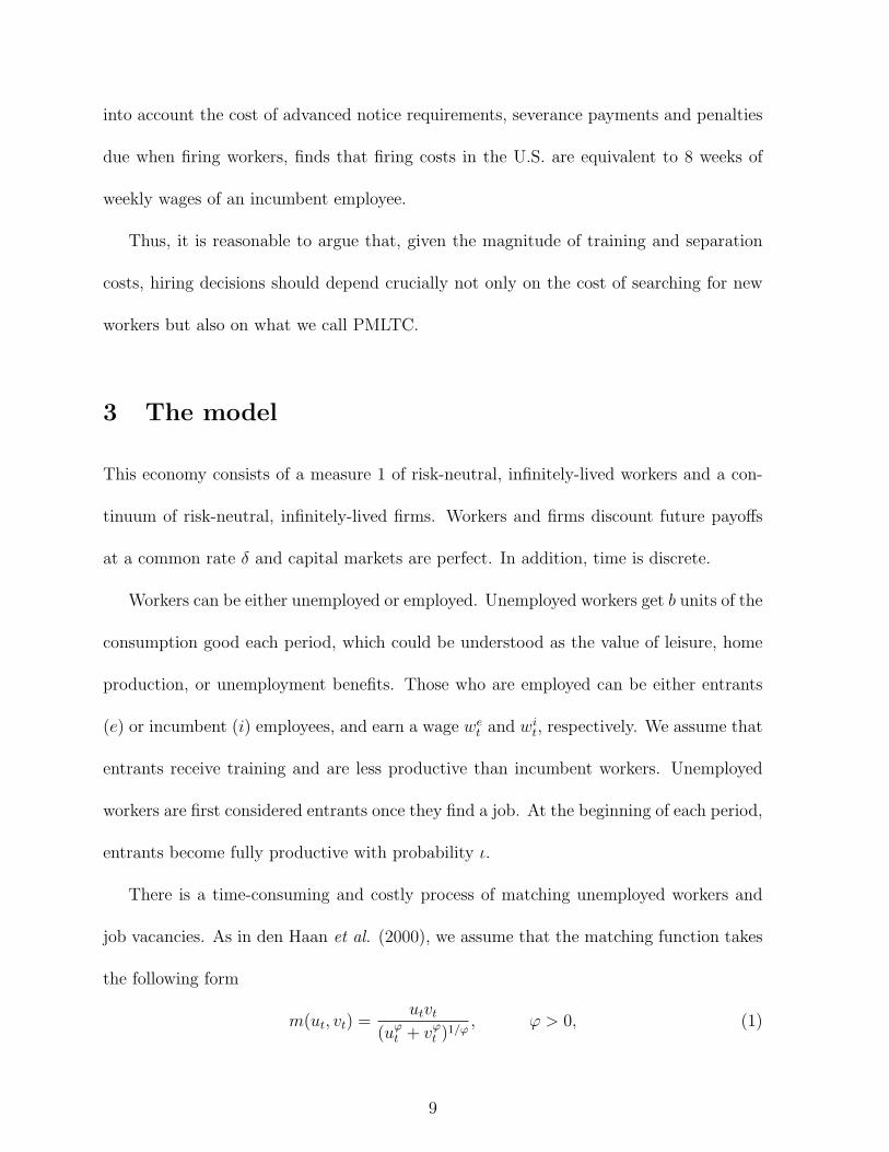
into account the cost of advanced notice requirements, severance payments and penalties

due when firing workers, finds that firing costs in the U.S. are equivalent to 8 weeks of

weekly wages of an incumbent employee.

Thus, it is reasonable to argue that, given the magnitude of training and separation

costs, hiring decisions should depend crucially not only on the cost of searching for new

workers but also on what we call PMLTC.

3 The model

This economy consists of a measure 1 of risk-neutral, infinitely-lived workers and a con-

tinuum of risk-neutral, infinitely-lived firms. Workers and firms discount future payoffs

at a common rate δ and capital markets are perfect. In addition, time is discrete.

Workers can be either unemployed or employed. Unemployed workers get b units of the

consumption good each period, which could be understood as the value of leisure, home

production, or unemployment benefits. Those who are employed can be either entrants

(e) or incumbent (i) employees, and earn a wage wet and wi

t, respectively. We assume that

entrants receive training and are less productive than incumbent workers. Unemployed

workers are first considered entrants once they find a job. At the beginning of each period,

entrants become fully productive with probability ι.

There is a time-consuming and costly process of matching unemployed workers and

job vacancies. As in den Haan et al. (2000), we assume that the matching function takes

the following form

m(ut, vt) =utvt

(uϕt + vϕ

t )1/ϕ, ϕ > 0, (1)

9

where ut denotes the unemployment rate and vt are vacancies. This constant-return-

to-scale matching function ensures that ratios m(ut, vt)/ut and m(ut, vt)/vt lie between

0 and 1. Due to the CRS assumption they only depend on the vacancy-unemployment

ratio θt. The former represents the probability at which unemployed workers meet jobs,

f(θt) = m(1, 1/θt). Similarly, the latter denotes the probability at which vacancies meet

workers, q(θt) = m(θt, 1).

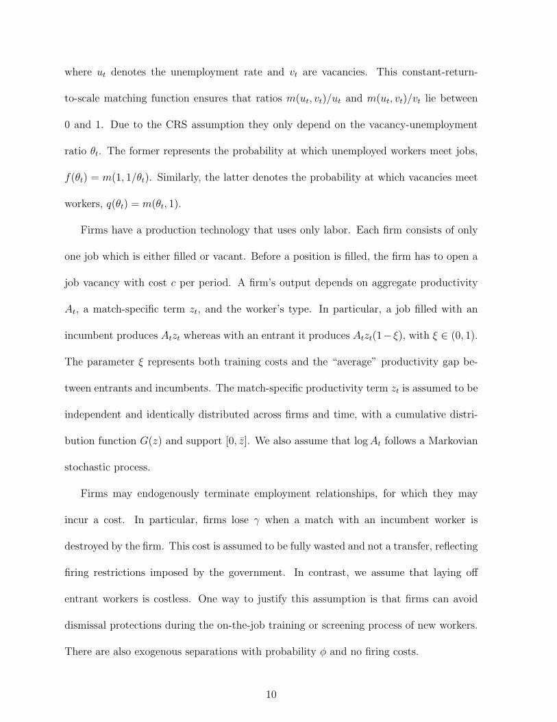
Firms have a production technology that uses only labor. Each firm consists of only

one job which is either filled or vacant. Before a position is filled, the firm has to open a

job vacancy with cost c per period. A firm’s output depends on aggregate productivity

At, a match-specific term zt, and the worker’s type. In particular, a job filled with an

incumbent produces Atzt whereas with an entrant it produces Atzt(1− ξ), with ξ ∈ (0, 1).

The parameter ξ represents both training costs and the “average” productivity gap be-

tween entrants and incumbents. The match-specific productivity term zt is assumed to be

independent and identically distributed across firms and time, with a cumulative distri-

bution function G(z) and support [0, z]. We also assume that log At follows a Markovian

stochastic process.

Firms may endogenously terminate employment relationships, for which they may

incur a cost. In particular, firms lose γ when a match with an incumbent worker is

destroyed by the firm. This cost is assumed to be fully wasted and not a transfer, reflecting

firing restrictions imposed by the government. In contrast, we assume that laying off

entrant workers is costless. One way to justify this assumption is that firms can avoid

dismissal protections during the on-the-job training or screening process of new workers.

There are also exogenous separations with probability φ and no firing costs.

10

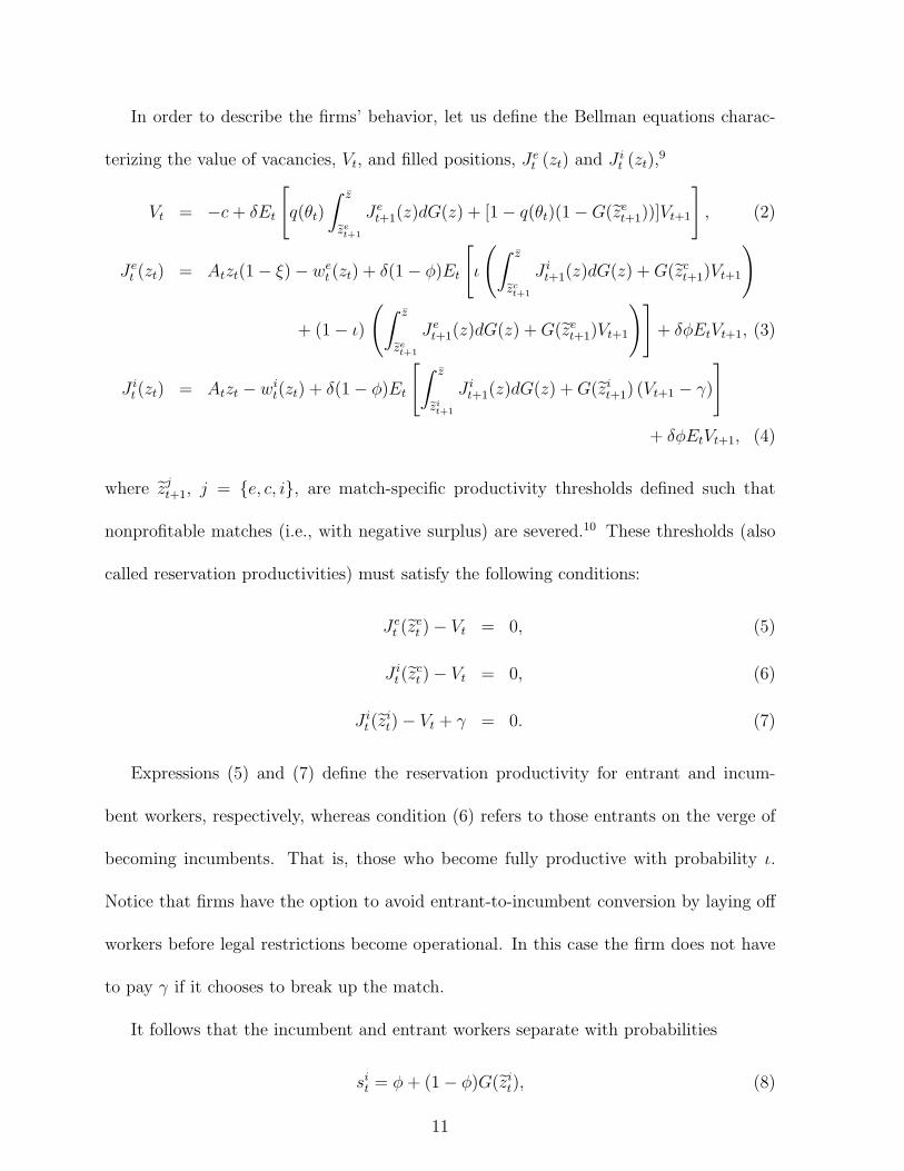
In order to describe the firms’ behavior, let us define the Bellman equations charac-

terizing the value of vacancies, Vt, and filled positions, Jet (zt) and J i

t (zt),9

Vt = −c + δEt

[q(θt)

∫ z

zet+1

Jet+1(z)dG(z) + [1− q(θt)(1−G(ze

t+1))]Vt+1

], (2)

Jet (zt) = Atzt(1− ξ)− we

t (zt) + δ(1− φ)Et

[ι

(∫ z

zct+1

J it+1(z)dG(z) + G(zc

t+1)Vt+1

)

+ (1− ι)

(∫ z

zet+1

Jet+1(z)dG(z) + G(ze

t+1)Vt+1

)]+ δφEtVt+1, (3)

J it (zt) = Atzt − wi

t(zt) + δ(1− φ)Et

[∫ z

zit+1

J it+1(z)dG(z) + G(zi

t+1) (Vt+1 − γ)

]

+ δφEtVt+1, (4)

where zjt+1, j = {e, c, i}, are match-specific productivity thresholds defined such that

nonprofitable matches (i.e., with negative surplus) are severed.10 These thresholds (also

called reservation productivities) must satisfy the following conditions:

Jet (z

et )− Vt = 0, (5)

J it (z

ct )− Vt = 0, (6)

J it (z

it)− Vt + γ = 0. (7)

Expressions (5) and (7) define the reservation productivity for entrant and incum-

bent workers, respectively, whereas condition (6) refers to those entrants on the verge of

becoming incumbents. That is, those who become fully productive with probability ι.

Notice that firms have the option to avoid entrant-to-incumbent conversion by laying off

workers before legal restrictions become operational. In this case the firm does not have

to pay γ if it chooses to break up the match.

It follows that the incumbent and entrant workers separate with probabilities

sit = φ + (1− φ)G(zi

t), (8)

11

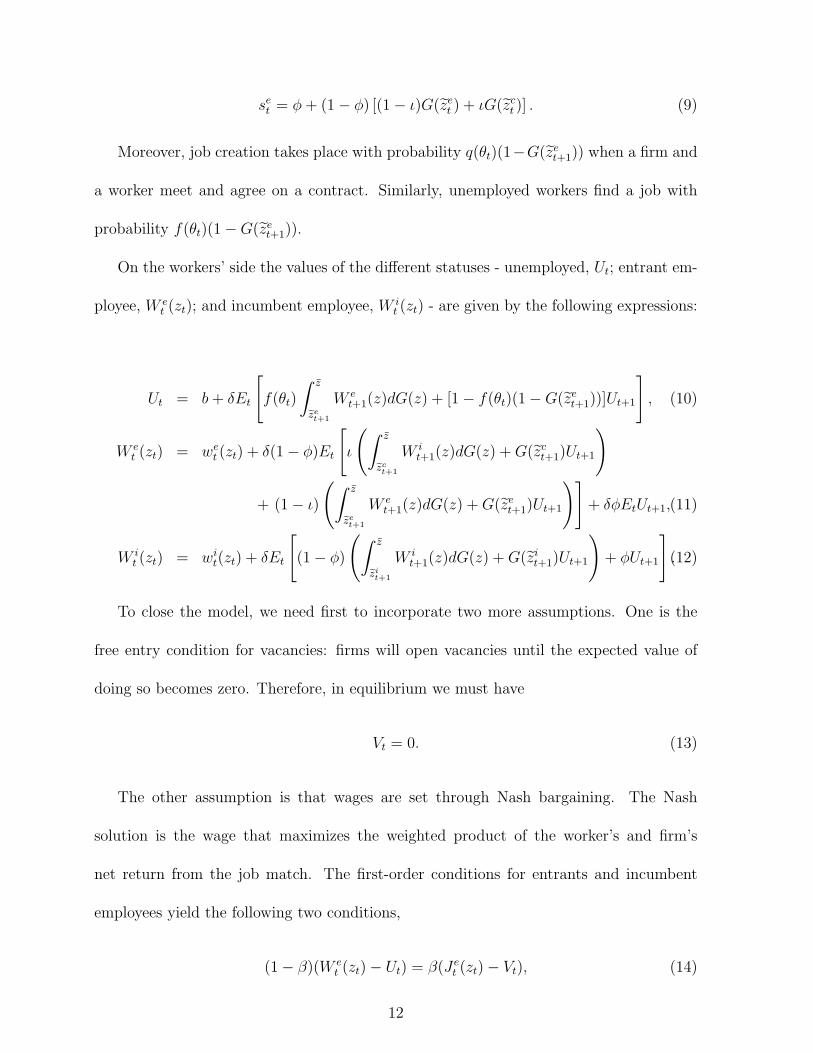
set = φ + (1− φ) [(1− ι)G(ze

t ) + ιG(zct )] . (9)

Moreover, job creation takes place with probability q(θt)(1−G(zet+1)) when a firm and

a worker meet and agree on a contract. Similarly, unemployed workers find a job with

probability f(θt)(1−G(zet+1)).

On the workers’ side the values of the different statuses - unemployed, Ut; entrant em-

ployee, W et (zt); and incumbent employee, W i

t (zt) - are given by the following expressions:

Ut = b + δEt

[f(θt)

∫ z

zet+1

W et+1(z)dG(z) + [1− f(θt)(1−G(ze

t+1))]Ut+1

], (10)

W et (zt) = we

t (zt) + δ(1− φ)Et

[ι

(∫ z

zct+1

W it+1(z)dG(z) + G(zc

t+1)Ut+1

)

+ (1− ι)

(∫ z

zet+1

W et+1(z)dG(z) + G(ze

t+1)Ut+1

)]+ δφEtUt+1,(11)

W it (zt) = wi

t(zt) + δEt

[(1− φ)

(∫ z

zit+1

W it+1(z)dG(z) + G(zi

t+1)Ut+1

)+ φUt+1

].(12)

To close the model, we need first to incorporate two more assumptions. One is the

free entry condition for vacancies: firms will open vacancies until the expected value of

doing so becomes zero. Therefore, in equilibrium we must have

Vt = 0. (13)

The other assumption is that wages are set through Nash bargaining. The Nash

solution is the wage that maximizes the weighted product of the worker’s and firm’s

net return from the job match. The first-order conditions for entrants and incumbent

employees yield the following two conditions,

(1− β)(W et (zt)− Ut) = β(Je

t (zt)− Vt), (14)

12

(1− β)(W it (zt)− Ut) = β(J i

t (zt)− Vt + γ), (15)

where β ∈ (0, 1) denotes workers bargaining power relative to firms. Notice that the Nash

condition for incumbents (15) has an extra term γ. The interpretation is that the firm’s

threat point when negotiating with an incumbent employee is no longer the value of a

vacancy Vt but (Vt − γ) because now separation costs are relevant.

Using (2)-(15), we can now solve for the equilibrium wages as a function of the current

state Aitzt and θt,

wet (zt) = (1− β)b + βθtc + βAtzt(1− ξ)− δβι(1− φ)[1−G(zc

t+1)]γ, (16)

wit(zt) = (1− β)b + βθtc + βAtzt + β[1− δ(1− φ)]γ. (17)

Introducing PMLTC decreases entrants’ wages (16) by a fraction of both the training

costs and the separation costs. In contrast, the incumbent wage (17) is higher because

incumbents are fully productive workers and separation costs are now operational, which

increase their “implicit” bargaining power.

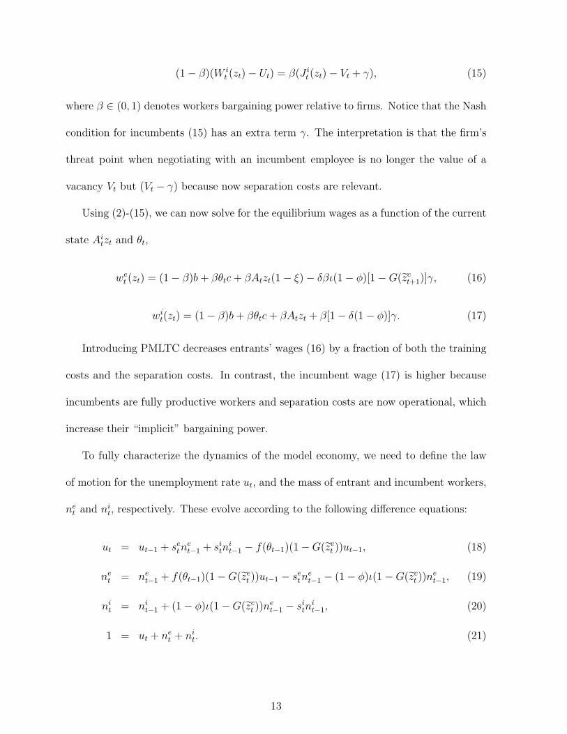
To fully characterize the dynamics of the model economy, we need to define the law

of motion for the unemployment rate ut, and the mass of entrant and incumbent workers,

net and ni

t, respectively. These evolve according to the following difference equations:

ut = ut−1 + setn

et−1 + si

tnit−1 − f(θt−1)(1−G(ze

t ))ut−1, (18)

net = ne

t−1 + f(θt−1)(1−G(zet ))ut−1 − se

tnet−1 − (1− φ)ι(1−G(zc

t ))net−1, (19)

nit = ni

t−1 + (1− φ)ι(1−G(zct ))n

et−1 − si

tnit−1, (20)

1 = ut + net + ni

t. (21)

13

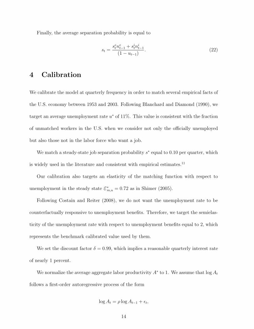
Finally, the average separation probability is equal to

st =se

tnet−1 + si

tnit−1

(1− ut−1). (22)

4 Calibration

We calibrate the model at quarterly frequency in order to match several empirical facts of

the U.S. economy between 1953 and 2003. Following Blanchard and Diamond (1990), we

target an average unemployment rate u∗ of 11%. This value is consistent with the fraction

of unmatched workers in the U.S. when we consider not only the officially unemployed

but also those not in the labor force who want a job.

We match a steady-state job separation probability s∗ equal to 0.10 per quarter, which

is widely used in the literature and consistent with empirical estimates.11

Our calibration also targets an elasticity of the matching function with respect to

unemployment in the steady state ε∗m,u = 0.72 as in Shimer (2005).

Following Costain and Reiter (2008), we do not want the unemployment rate to be

counterfactually responsive to unemployment benefits. Therefore, we target the semielas-

ticity of the unemployment rate with respect to unemployment benefits equal to 2, which

represents the benchmark calibrated value used by them.

We set the discount factor δ = 0.99, which implies a reasonable quarterly interest rate

of nearly 1 percent.

We normalize the average aggregate labor productivity A∗ to 1. We assume that log At

follows a first-order autoregressive process of the form

log At = ρ log At−1 + εt,

14

where εt is an i.i.d. N(0, σε) random variable. The parameters of the AR(1) process,

the autoregressive coefficient ρ and the standard deviation of the white noise process σε,

are calibrated to match the cyclical volatility (0.02) and persistence (0.88) of the average

U.S. labor productivity yt/(1− ut) between 1953 and 2003.12 Thus, we set ρ = 0.96 and

σε = 0.01.

Regarding the exogenous separation probability φ, we follow den Haan et al. (2000),

and interpret exogenous separations as worker-initiated separations. Hence, only endoge-

nous separations are associated with the layoff rate. According to evidence from the Job

Opening Labor Turnover Survey (JOLTS) shown by Davis, Faberman, and Haltiwanger

(2006), and from the Census’ Survey of Income and Program Participation (SIPP) shown

by Nagypal (2004), layoffs represent on average about 35% of total separations. Thus, we

set φ = 0.065, which is close to the one used by den Haan et al. (2000).

We now turn to the labor turnover cost parameters c, ι, ξ, and γ. As mentioned in

Section 2, the 1982 EOPP and the 1992 SBA surveys estimate total hiring costs to be

about 4.3 percent of the quarterly compensation of a new hired worker. Therefore, we set

c such that in the steady state it is equal to 0.043we∗.

Barron, Berger and Black (1997) document the average time that a newly hired worker

takes to become fully trained according to two surveys: the above mentioned 1982 EOPP

survey and the 1992 Small Business Administration (SBA) survey. They find that it takes

on average between 20.2 and 22.2 weeks to become fully trained.13 The 1992 SBA survey

also suggests that the most intense training period is the first three months on the job.

They estimate that around 70 percent of training spells are finished within this period.

However, a new employee needs more than on-the-job training to fill the productivity

15

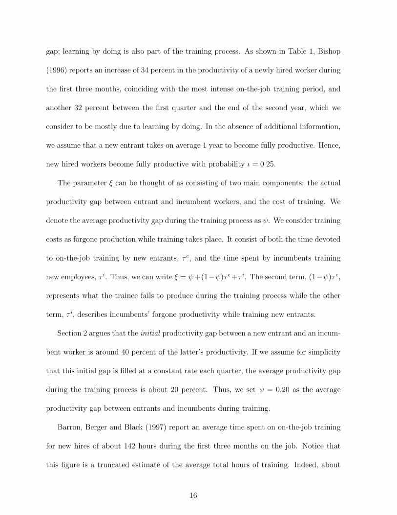
gap; learning by doing is also part of the training process. As shown in Table 1, Bishop

(1996) reports an increase of 34 percent in the productivity of a newly hired worker during

the first three months, coinciding with the most intense on-the-job training period, and

another 32 percent between the first quarter and the end of the second year, which we

consider to be mostly due to learning by doing. In the absence of additional information,

we assume that a new entrant takes on average 1 year to become fully productive. Hence,

new hired workers become fully productive with probability ι = 0.25.

The parameter ξ can be thought of as consisting of two main components: the actual

productivity gap between entrant and incumbent workers, and the cost of training. We

denote the average productivity gap during the training process as ψ. We consider training

costs as forgone production while training takes place. It consist of both the time devoted

to on-the-job training by new entrants, τ e, and the time spent by incumbents training

new employees, τ i. Thus, we can write ξ = ψ+(1−ψ)τ e +τ i. The second term, (1−ψ)τ e,

represents what the trainee fails to produce during the training process while the other

term, τ i, describes incumbents’ forgone productivity while training new entrants.

Section 2 argues that the initial productivity gap between a new entrant and an incum-

bent worker is around 40 percent of the latter’s productivity. If we assume for simplicity

that this initial gap is filled at a constant rate each quarter, the average productivity gap

during the training process is about 20 percent. Thus, we set ψ = 0.20 as the average

productivity gap between entrants and incumbents during training.

Barron, Berger and Black (1997) report an average time spent on on-the-job training

for new hires of about 142 hours during the first three months on the job. Notice that

this figure is a truncated estimate of the average total hours of training. Indeed, about

16

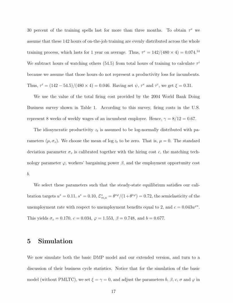
30 percent of the training spells last for more than three months. To obtain τ e we

assume that these 142 hours of on-the-job training are evenly distributed across the whole

training process, which lasts for 1 year on average. Thus, τ e = 142/(480 × 4) = 0.074.14

We subtract hours of watching others (54.5) from total hours of training to calculate τ i

because we assume that those hours do not represent a productivity loss for incumbents.

Thus, τ i = (142− 54.5)/(480× 4) = 0.046. Having set ψ, τ e and τ i, we get ξ = 0.31.

We use the value of the total firing cost provided by the 2004 World Bank Doing

Business survey shown in Table 1. According to this survey, firing costs in the U.S.

represent 8 weeks of weekly wages of an incumbent employee. Hence, γ = 8/12 = 0.67.

The idiosyncratic productivity zt is assumed to be log-normally distributed with pa-

rameters (µ, σz). We choose the mean of log zt to be zero. That is, µ = 0. The standard

deviation parameter σz is calibrated together with the hiring cost c, the matching tech-

nology parameter ϕ, workers’ bargaining power β, and the employment opportunity cost

b.

We select these parameters such that the steady-state equilibrium satisfies our cali-

bration targets u∗ = 0.11, s∗ = 0.10, ε∗m,u = θ∗ϕ/(1+θ∗ϕ) = 0.72, the semielasticity of the

unemployment rate with respect to unemployment benefits equal to 2, and c = 0.043we∗.

This yields σz = 0.170, c = 0.034, ϕ = 1.553, β = 0.748, and b = 0.677.

5 Simulation

We now simulate both the basic DMP model and our extended version, and turn to a

discussion of their business cycle statistics. Notice that for the simulation of the basic

model (without PMLTC), we set ξ = γ = 0, and adjust the parameters b, β, c, σ and ϕ in

17

order to maintain our calibration target values.15 In this case, we set b = 0.60, β = 0.837,

c = 0.0565, σz = 0.47 and ϕ = 1.891.

We simulate the model presented above 10,000 times. Each time we simulate the

economy for 1,212 “quarters” and throw away the first 1,000 of them in order to obtain

the U.S. post Second World War period (212 quarters between 1951-2003). We detrend

the generated data using an HP filter with 105 smoothing parameter and, finally, we

calculate the standard deviations, autocorrelation coefficients and correlation matrix.

5.1 Results

Table 3 presents the summary statistics of the U.S. labor market. Tables 4 and 5 show

the simulation results of the model without and with PMLTC, respectively.16

The most important difference between both versions of the model lies in the volatility

of vacancies and, consequently, θ and the job finding rate f(θ). As in Shimer (2005)

(see his Table 5), we find that in the standard model with job destruction and without

training and separation costs the variables above show relatively low variability, with

standard deviations that are at most 20 percent as volatile as in U.S. data. In contrast,

our extended version of the DMP model notably increases those standard deviations.

The volatility of v (0.062), θ (0.105) and f(θ) (0.030) are more than two times higher

than what we observe in the standard model without PMLTC (0.007, 0.043 and 0.015,

respectively). The standard deviation of unemployment also increases but in a smaller

magnitude (from 0.039 to 0.049). In spite of the larger fluctuations predicted by our

model, it still underestimates the U.S. labor market volatility by a considerable margin.

In turn, vacancies become more persistent with PMLTC. The autocorrelation coeffi-

18

cient is 0.738 compared to 0.123 in the standard model and 0.940 in the data. Similarly,

the negative correlation between vacancies and unemployment is considerably increased

from -0.377 to -0.808, which comes much closer to the observed correlation of -0.894 in

the U.S. Finally, the standard deviation of the job destruction rate s is the nearly the

same in both models and 60 percent smaller than the value observed in the data (0.075).

5.2 Discussion

To understand why the cyclical fluctuations of vacancies and unemployment increase when

we introduce PMLTC into the model we need to consider the total match surplus of a new

entrant. Let us define the new entrant’s match surplus as Set (zt) = Je

t (zt)−Vt+W et (zt)−Ut.

After some substitutions we obtain the following expression:

Set (zt) = Atzt(1− ξ)− b− ιδ(1− φ)(1−G(zc

t+1))γ − δβf(θt)Et

[∫ z

zet+1

Set+1(z)dG(z)

]

+(1− φ)δ

(ιEt

[∫ z

zct+1

Sit+1(z)dG(z)

]+ (1− ι)Et

[∫ z

zet+1

Set+1(z)dG(z)

]),(23)

where Sit(zt) = J i

t (zt) − Vt + γ + W it (zt) − Ut represents the incumbent’s match surplus.

Notice that for every productivity level Atzt the match surplus of a new entrant is lower

when we account for training ξ and firing costs γ. However, since our parameterizations

of the extended and the standard models yield different parameter values for σ, b, c,

ϕ and β, a more meaningful comparison between both versions of the model is to look

at their calibrated match surplus Se across different levels of aggregate productivity A.

Figure 1 shows that Se is lower for every level of A when PMLTC are accounted for. This

implies that in the extended model productivity shocks have a relatively greater impact

on Set (zt) and, consequently, on the value of a newly filled position Je

t (zt) = (1−β)Set (zt).

19

As Hornstein, Krusell and Violante (2005) point out, given the equilibrium job creation

condition, (1 − β)δEt

[∫ z

zet+1

Set+1(z)dG(z)

]= c/q(θt), a larger percentage change in Se

induces a greater response in labor market tightness θ.17 Hence a higher volatility of

vacancies and unemployment. Figures 2 and 3 show the response of the conditional mean

of Set , E[Se

t (z)|z ≥ zet ], to a 1 percent increase in At = A∗ with and without PMLTC. On

impact, the average surplus increases by more than two times in the former case relative

to the latter, magnifying the initial response of labor market variables.

According to Costain and Reiter (2008), the standard matching model with exogenous

job destruction can generate sufficiently large cyclical fluctuations in unemployment, or

a sufficiently small response of unemployment to unemployment benefits, but it cannot

do both. As stressed by these authors, this result depends crucially on the surplus of a

match. The smaller this surplus is, the higher the response of the job-finding probability

f(θ) to changes in UB. Given the job destruction probability, unemployment becomes

more sensitive.

This puzzle is still present with endogenous job destruction because higher levels of UB

not only increase unemployment through reductions in f(θ) but also through increments

in s. However, our extended model with PMLTC leads to a greater amplification of

productivity shocks without introducing “unrealistic” sensitivity to policy changes. The

origin of this result lies in the lower response of the job destruction probability to an

increase in UB.

This point can be verified in Table 6. On the one hand, Se is about 50 percent lower

when the model accounts for PMLTC than in the case when these costs are omitted. As

a result, the elasticity of f(θ) with respect to the employment opportunity cost b in the

20

steady state, ε∗f,b, is about two times higher (in absolute value) in the former case (-1.1

with respect to -0.5 when PMLTC are excluded). On the other hand, the elasticity of job

destruction probability with respect to b, ε∗s,b, is more than 3 times higher when there are

no training and separation costs in the model (2.1 with PMLTC versus 0.6). Intuitively,

when firing a worker becomes more costly, firms choose to keep relatively more employees

in response to an increase in b. Thus, the elasticity of unemployment with respect to b

changes only slightly from 2.2 to 1.8.

It is well known that endogenous job destruction tends to induce positive correlation

between unemployment and vacancies in the DMP model. For example, Shimer (2005)

shows a correlation coefficient of 0.95 between these two variables when there are only

stochastic shocks to the job destruction rate. He also shows that the model with labor

productivity shocks and a constant job destruction rate is quantitatively consistent with

the observed correlation coefficient in the data (-0.894). Costain and Reiter (2008) show

similar results. Our simulated results show that our extended model is also quantitatively

consistent with the observed downward-sloping Beveridge curve (the simulated correlation

coefficient is -0.809). As before, this result takes place because training and separation

costs make job creation much more sensitive than job destruction. Hence, employment

dynamics is mostly driven by the former. To understand why this induces a more negative

correlation, let us think about the opposite case where separations play a bigger role

in employment fluctuations. In that case, when a positive productivity shock hits the

economy, firms lay off fewer workers which reduces unemployment but dampens vacancy

creation because firms do not need to recruit as many workers now.

Finally, notice that in our extended version of the model the correlation coefficient

21

between the average wage and labor productivity remains almost as high as in the basic

model because there is no change in the Nash Bargaining scheme. Therefore, we can

argue that without introducing wage rigidities it is possible to improve the performance

of the model.

5.3 Endogenous job destruction and the amplification mecha-

nism

To study how endogenous separations affect vacancies and unemployment fluctuations, we

now reduce to a minimun the response of job destruction to aggregate productivity shocks

by making all separations exogenous in the steady state. Thus, we set the exogenous

separation probability φ to 0.10. This does not necessarily mean that all separations will

be exogenous. Out of the steady state, particularly for low levels of aggregate productivity,

there could still be endogenous separations.

We also recalibrate parameters b, β, c, σ and ψ in order to maintain our calibration

target values. In this case, we set b = 0.776, β = 0.564, c = 0.0424, σ = 0.071 and

ψ = 1.551. The simulation results are shown in Table 7.

Compared with our baseline simulation results in Table 5, the volatility of vacancies

nearly doubles (from 0.062 to 0.115). In contrast, the standard deviation of unemploy-

ment is reduced by 28% (from 0.049 to 0.036). As a result, the volatility of labor market

tightness increases from 0.105 to 0.146. Thus, a higher response of endogenous job de-

struction to aggregate shocks significantly dampens the response of vacancies and labor

market tightness.

22

6 Conclusions

In this study we argue that introducing post-match labor turnover costs in the standard

DMP matching model with endogenous job destruction helps increase the labor market

volatility in response to labor productivity shocks of reasonable magnitude.

In particular, the simulation of our model shows that with reasonable parameter values

for training and separation costs the volatility of vacancies and labor market tightness

more than doubles with respect to the model with no PMLTC. Moreover, in contrast to

the standard matching model with endogenous job destruction, our extended model comes

close to matching the observed negative relationship between vacancies and unemployment

because job creation becomes relatively more sensitive to aggregate productivity shocks

than job destruction.

The crucial reason behind this result is the lower value of a new match since (i)

entrants need training before being fully productive as incumbent employees, and (ii)

firms may become liable to separation costs in the future. This amplifies the volatility

of the model because productivity shocks account for a larger fraction of the value of a

newly filled position. Therefore, firms’ reaction, namely job creation, is more volatile.

Thus, both vacancies and labor market tightness fluctuate more over the business cycle.

Finally, considering Costain and Reiter’s (2008) observation, our matching model gen-

erates not only larger cyclical fluctuations in labor market variables but also a sufficiently

small response of unemployment to changes in unemployment benefits. This result is

driven by how PMLTC affect the elasticity of both the job finding probability and the

separation probability with respect to the employment opportunity cost. On the one

hand, the elasticity of the former increases with training and separation costs as the sur-

23

plus of a new match falls. On the other hand, higher PMLTC make job destruction less

sensitive to policy changes. These two opposing forces counterbalance each other with

respect to their impact on the unemployment rate.

Notes

1See Hornstein, Krusell and Violante (2005) for a similar mechanism at work in the standard model

when labor productivity is close to the value of being unemployed.

2Shimer (2005) and Costain and Reiter (2008) point out that endogenous job destruction in the spirit

of Mortensen and Pissarides (1994) deteriorates the Beveridge curve.

3See for example, Ahr and Ahr (2000).

4See Table 1 from Barron, Berger and Black (1997).

5See Table 1 from Dolfin (2006).

6The EOPP project contains a set of four questions concerning various types of on-the-job training

related to the total number of hours spent during the first three months of employment (a) by specially

trained personnel providing formal training to the most recently hired worker, (b) by line supervisors

providing the new worker with informal individualized training and extra supervision and (d) by the

worker watching others perform tasks. Contrary to the EOPP project, others surveys such as the Current

Population Survey (CPS) and the National Longitudinal Survey of Youth (NLSY) have received criticism

since they lack all or most of the informal training information. See Loewenstein and Spletzer (1994) for

a detailed analysis.

7The 1992 Small Business Administration (SBA) survey is a more recent survey that reports a similar

number of hours spent on on-the-job training during the first three months of employment (150 hours).

See Barron, Berger and Black (1997).

8Using also the 1982 EOPP survey, Dolfin (2006) finds that “[t]he average new employee spends 201

hours [...] in training activities during the first three months of work, while other employees spend

on average 146 hours [...] training her. The total average cost of these 347 manhours to the firm is

24

approximately $2,119. This figure is within the range found by other studies, and may understate the

total cost of training a new worker if the training period exceeds three months.” So, if anything, our

estimate of training costs is rather conservative.

9For exposition reasons, we omit writing the aggregate state variables {At, θt} as arguments of these

value functions.

10 Since the value of a match is increasing in zt, we can prove that there exists a threshold zt ∈ [0, z]

below which matches are no longer profitable.

11See, for example, Shimer (2005), den Haan et al. (2000).

12Total output yt is equal to yt = Atzitn

i + Atzet (1 − ξ)ne, where zj = E[z|z ≥ zj ]. As in Shimer

(2005), the average labor productivity is the seasonally adjusted real average output per person in the

non-farm business sector, constructed by the Bureau of Labor Statistics (BLS) from the National Income

and Product Accounts and the Current Employment Statistics. It is reported in logs as deviations from

an HP trend with a smoothing parameter of 105.

13For details, see Table 3.4 in Barron, Berger and Black (1997).

14We assume that every quarter workers work 480 hours, equivalent to 40 hours per week.

15Notice that as ξ and γ approach zero, ι becomes irrelevant since we and Je tend to approach wi and

J i, respectively.

16Table 3 reproduces Table 1 from Shimer (2004, 2005) available at the AER and Shimer’s webpage.

17The equilibrium job creation condition comes from equations (2) and (13).

References

Ahr, Paul R. and Thomas Ahr. (2000) Overturn Turnover. Causeway Publishing

Company.

Barron, John M., Mark C. Berger, and Dan A. Black (1997) On-the-Job Training.

W.E. Upjohn Institute for Employment Research.

Bishop, John H. (1996) What We Know About the Employer-Provided Training:

25

A Review of Literature. Center for Advanced Human Resources Studies, Working

Paper 96-09.

Blanchard, Olivier and Diamond Peter (1990) The Cyclical Behavior of the Gross

Flows of U.S. Workers, Brookings Papers on Economic Activity 2, 85-155.

Blanchard, Olivier and Augustin Landier (2000) The Perverse Effects of Partial

Labor Market Reform: Fixed Term Contracts in France., The Economic Journal

112, F214-F244.

Cahuc, Pierre and Fabien Postel-Vinay (2002) Temporary Jobs, Employment

Protection and Labor Market Performance. Labour Economics 9, 63-91.

Costain, James S. and Reiter Michael (2008) Business Cycles, Unemployment

Insurance, and the Calibration of Matching Models. Journal of Economic Dynamics

and Control, 32, 1120-1155.

Davis, Steven Faberman, Faberman Janson and Haltiwanger John (2006) Flow

Approach to Labor Markets: New Data Sources and Micro-Macro Links, National

Bureau of Economic Research, working Paper No. 12167.

den Haan, Wouter, Ramey Garey and Watson Joel (2000) Job Destruction and

Propagation of Shocks, American Economic Review 90, 482-498.

Diamond, Peter (1982) Wage Determination and Efficiency in Search Equilibrium.

Review of Economic Studies 49, 217-227.

Dolfin, Sarah (2006) An Examination of Firms’ Employment Costs. Applied Eco-

nomics 38, 861-878.

Hagedorn, Marcus and Iouri Manovski (2008) The Cyclical Behavior of Equilibrium

Unemployment and Vacancies Revisited. American Economic Review, Forthcoming.

26

Hall, Robert E. (2005) Employment Fluctuations with Equilibrium Wage Stickiness.

American Economic Review 95, 50-65.

Hornstein, Andreas, Per Krusell, and Gianluca Violante (2005) Unemployment and

Vacancy Fluctuations in the Matching Model: Inspecting the Mechanism. Federal

Reserve Bank of Richmond Economic Quarterly 91, 19-51.

Loewenstein, Mark A. and James R. Spletzer (1994) Informal Training: A Review of

Existing Data and Some New Evidence. Bureau of Labor Statistics Working Paper

254.

Mortensen, Dale (1982) The Matching Process as a Non-Cooperative/Bargaining

Game. in Mc Call, J. (ed.), The Economics Information and Uncertanty. Chicago,

University of Chicago.

Mortensen, Dale and Eva Nagypal (2007) More on Unemployment and Vacancy

Fluctuations. Review of Economic Dynamics 10, 327-347.

Mortensen, Dale and Christopher Pissarides (1994) Job Creation and Job Destruc-

tion in the Theory of Unemployment, Review of Economic Studies 61, 397-415.

Mortensen, Dale and Christopher Pissarides (1999) New Developments in Models

of Search in the Labor Market. in Ashenfelter O. and Card D. (eds.). Handbook of

Labor Economics 3, 2567-2627. North-Holland.

Nagypal, Eva (2004): Worker Reallocation over the Business Cycle: The Importance

of Job-to-Job Transitions, mimeo, Northwestern University.

Pissarides, Christopher (1985) Short-Run Equilibrium Dynamics of Unemployment,

Vacancies, and Real Wages. American Economic Review 54, 1319-1338.

Shimer, Robert (2005) The Cyclical Behavior of Equilibrium Unemployment and

27

Vacancies. American Economic Review 95, 25-49.

Shimer, Robert (2004): The Consequences of Rigid Wages in Search Models. Journal

of European Economic Association (Papers and Proceedings) 2, 469-479.

Wasmer, Etienne (1999) Competition for jobs in a growing economy and the

emergence of dualism in employment. The Economic Journal 109, 349-371.

28

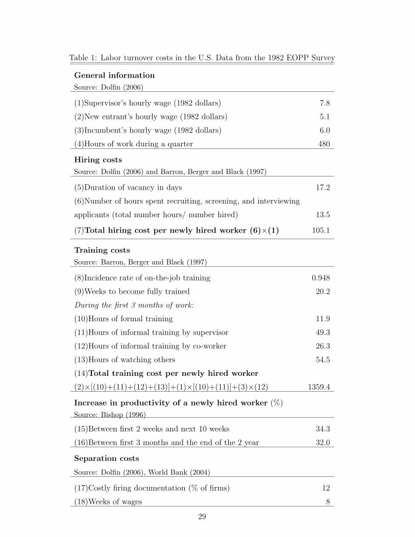
Table 1: Labor turnover costs in the U.S. Data from the 1982 EOPP Survey

General information

Source: Dolfin (2006)

(1)Supervisor’s hourly wage (1982 dollars) 7.8

(2)New entrant’s hourly wage (1982 dollars) 5.1

(3)Incumbent’s hourly wage (1982 dollars) 6.0

(4)Hours of work during a quarter 480

Hiring costs

Source: Dolfin (2006) and Barron, Berger and Black (1997)

(5)Duration of vacancy in days 17.2

(6)Number of hours spent recruiting, screening, and interviewing

applicants (total number hours/ number hired) 13.5

(7)Total hiring cost per newly hired worker (6)×(1) 105.1

Training costs

Source: Barron, Berger and Black (1997)

(8)Incidence rate of on-the-job training 0.948

(9)Weeks to become fully trained 20.2

During the first 3 months of work:

(10)Hours of formal training 11.9

(11)Hours of informal training by supervisor 49.3

(12)Hours of informal training by co-worker 26.3

(13)Hours of watching others 54.5

(14)Total training cost per newly hired worker

(2)×[(10)+(11)+(12)+(13)]+(1)×[(10)+(11)]+(3)×(12) 1359.4

Increase in productivity of a newly hired worker (%)

Source: Bishop (1996)

(15)Between first 2 weeks and next 10 weeks 34.3

(16)Between first 3 months and the end of the 2 year 32.0

Separation costs

Source: Dolfin (2006), World Bank (2004)

(17)Costly firing documentation (% of firms) 12

(18)Weeks of wages 8

29

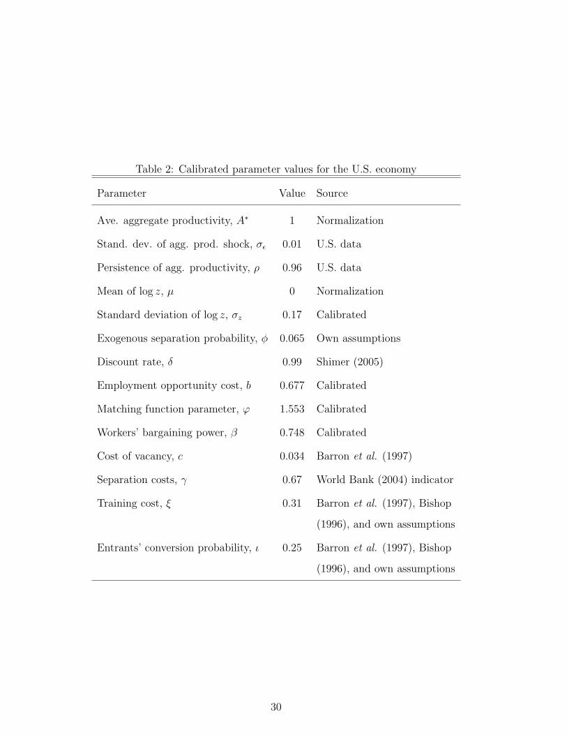
Table 2: Calibrated parameter values for the U.S. economy

Parameter Value Source

Ave. aggregate productivity, A∗ 1 Normalization

Stand. dev. of agg. prod. shock, σε 0.01 U.S. data

Persistence of agg. productivity, ρ 0.96 U.S. data

Mean of log z, µ 0 Normalization

Standard deviation of log z, σz 0.17 Calibrated

Exogenous separation probability, φ 0.065 Own assumptions

Discount rate, δ 0.99 Shimer (2005)

Employment opportunity cost, b 0.677 Calibrated

Matching function parameter, ϕ 1.553 Calibrated

Workers’ bargaining power, β 0.748 Calibrated

Cost of vacancy, c 0.034 Barron et al. (1997)

Separation costs, γ 0.67 World Bank (2004) indicator

Training cost, ξ 0.31 Barron et al. (1997), Bishop

(1996), and own assumptions

Entrants’ conversion probability, ι 0.25 Barron et al. (1997), Bishop

(1996), and own assumptions

30

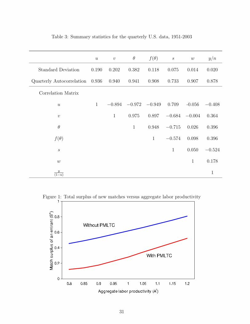
Table 3: Summary statistics for the quarterly U.S. data, 1951-2003

u v θ f(θ) s w y/n

Standard Deviation 0.190 0.202 0.382 0.118 0.075 0.014 0.020

Quarterly Autocorrelation 0.936 0.940 0.941 0.908 0.733 0.907 0.878

Correlation Matrix

u 1 −0.894 −0.972 −0.949 0.709 -0.056 −0.408

v 1 0.975 0.897 −0.684 −0.004 0.364

θ 1 0.948 −0.715 0.026 0.396

f(θ) 1 −0.574 0.098 0.396

s 1 0.050 −0.524

w 1 0.178

y(1−u)

1

Figure 1: Total surplus of new matches versus aggregate labor productivity

31

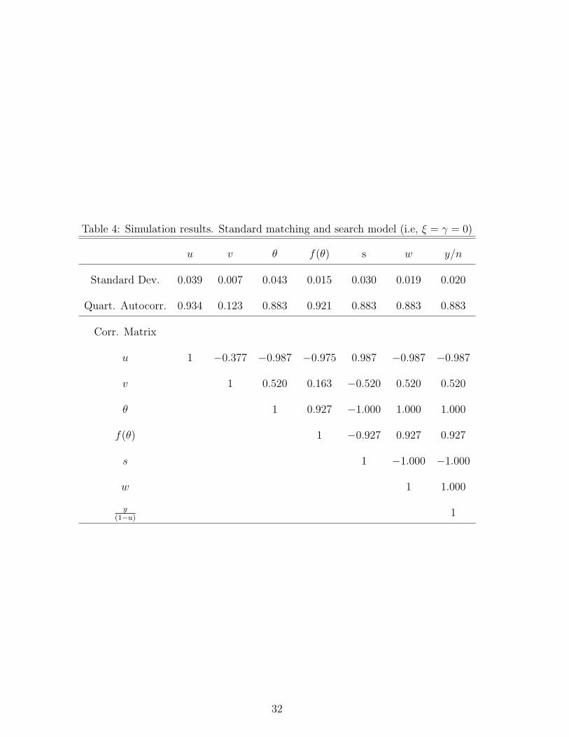
Table 4: Simulation results. Standard matching and search model (i.e, ξ = γ = 0)

u v θ f(θ) s w y/n

Standard Dev. 0.039 0.007 0.043 0.015 0.030 0.019 0.020

Quart. Autocorr. 0.934 0.123 0.883 0.921 0.883 0.883 0.883

Corr. Matrix

u 1 −0.377 −0.987 −0.975 0.987 −0.987 −0.987

v 1 0.520 0.163 −0.520 0.520 0.520

θ 1 0.927 −1.000 1.000 1.000

f(θ) 1 −0.927 0.927 0.927

s 1 −1.000 −1.000

w 1 1.000

y(1−u)

1

32

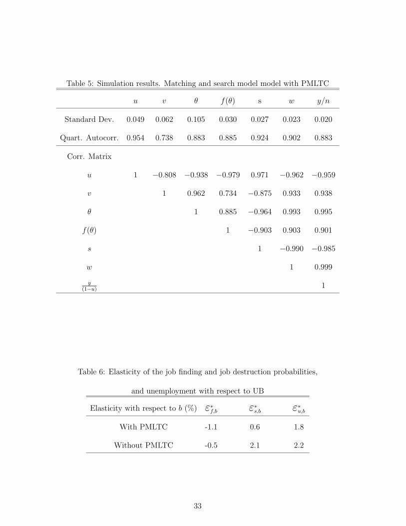
Table 5: Simulation results. Matching and search model model with PMLTC

u v θ f(θ) s w y/n

Standard Dev. 0.049 0.062 0.105 0.030 0.027 0.023 0.020

Quart. Autocorr. 0.954 0.738 0.883 0.885 0.924 0.902 0.883

Corr. Matrix

u 1 −0.808 −0.938 −0.979 0.971 −0.962 −0.959

v 1 0.962 0.734 −0.875 0.933 0.938

θ 1 0.885 −0.964 0.993 0.995

f(θ) 1 −0.903 0.903 0.901

s 1 −0.990 −0.985

w 1 0.999

y(1−u)

1

Table 6: Elasticity of the job finding and job destruction probabilities,

and unemployment with respect to UB

Elasticity with respect to b (%) ε∗f,b ε∗s,b ε∗u,b

With PMLTC -1.1 0.6 1.8

Without PMLTC -0.5 2.1 2.2

33

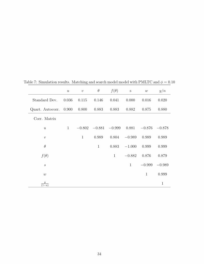
Table 7: Simulation results. Matching and search model model with PMLTC and φ = 0.10

u v θ f(θ) s w y/n

Standard Dev. 0.036 0.115 0.146 0.041 0.000 0.016 0.020

Quart. Autocorr. 0.900 0.800 0.883 0.883 0.882 0.875 0.880

Corr. Matrix

u 1 −0.802 −0.881 −0.999 0.881 −0.876 −0.878

v 1 0.989 0.804 −0.989 0.989 0.989

θ 1 0.883 −1.000 0.999 0.999

f(θ) 1 −0.882 0.876 0.879

s 1 −0.999 −0.989

w 1 0.999

y(1−u)

1

34

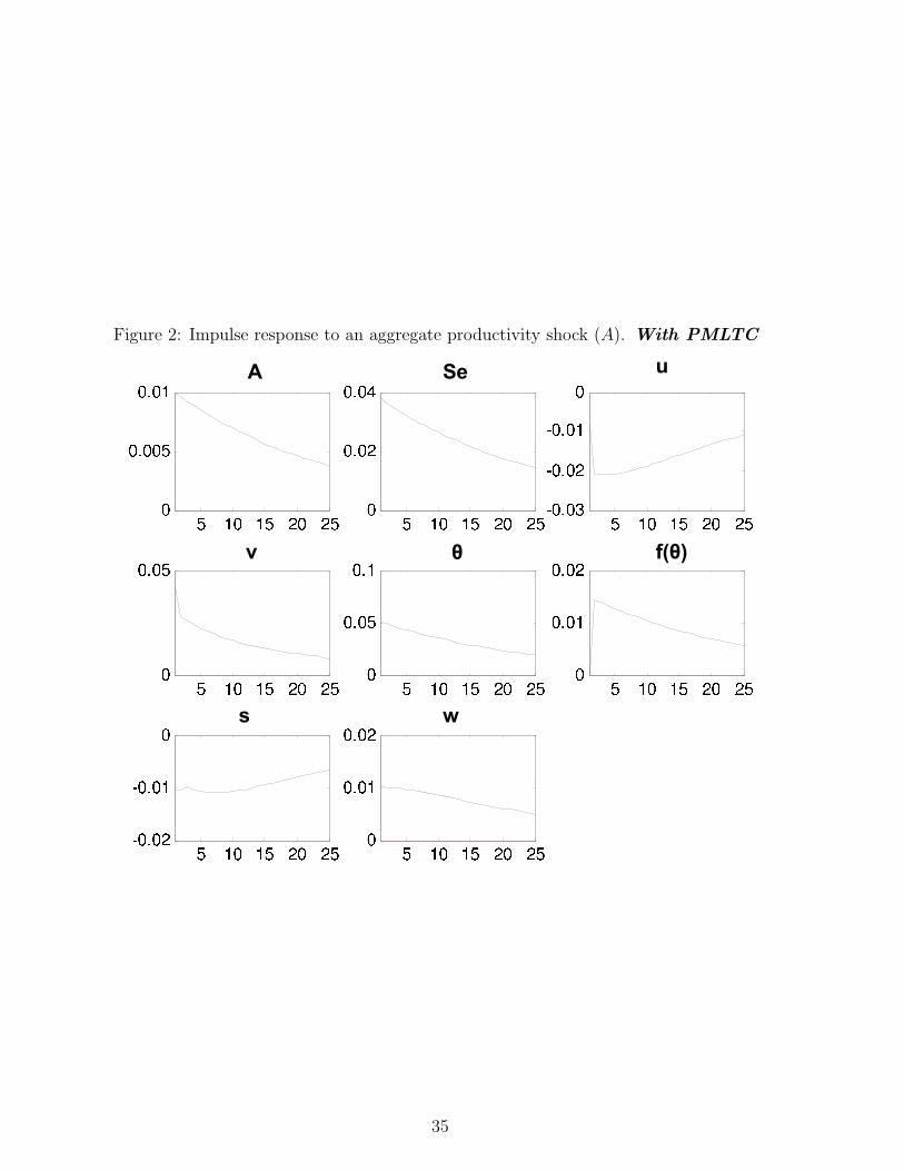
Figure 2: Impulse response to an aggregate productivity shock (A). With PMLTC

35

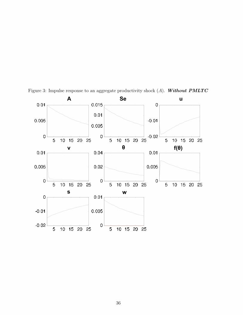
Figure 3: Impulse response to an aggregate productivity shock (A). Without PMLTC

36