knowledge discovery and data mining i - uni-muenchen.de · knowledge discovery and data mining i...
TRANSCRIPT

Ludwig-Maximilians-Universitat MunchenLehrstuhl fur Datenbanksysteme und Data Mining
Prof. Dr. Thomas Seidl
Knowledge Discovery and Data Mining I
Winter Semester 2018/19

Agenda
1. Introduction
2. Basics
3. Unsupervised Methods3.1 Frequent Pattern Mining3.2 Clustering
3.2.1 Partitioning Methods3.2.2 Probabilistic Model-Based Methods3.2.3 Density-Based Methods3.2.4 Mean-Shift3.2.5 Spectral Clustering3.2.6 Hierarchical Methods3.2.7 Evaluation3.2.8 Ensemble Clustering
3.3 Outlier Detection
4. Supervised Methods
5. Advanced Topics

What is Clustering?
Clustering
Grouping a set of data objects into clusters (=collections of dataobjects).
I Similar to one another within the same cluster
I Dissimilar to the objects in other clusters
Typical Usage
I As a stand-alone tool to get insight into data distribution
I As a preprocessing step for other algorithms
Unsupervised Methods Clustering January 25, 2019 189

General Applications of Clustering
I Preprocessing – as a data reduction (instead of sampling)I Image data bases (color histograms for filter distances)I Stream clustering (handle endless data sets for offline clustering)
I Pattern Recognition and Image ProcessingI Spatial Data Analysis:
I create thematic maps in Geographic Information Systems by clustering feature spacesI detect spatial clusters and explain them in spatial data mining
I Business Intelligence (especially market research)I WWW
I Documents (Web Content Mining)I Web-logs (Web Usage Mining)
I Biology, e.g. Clustering of gene expression data
Unsupervised Methods Clustering January 25, 2019 190
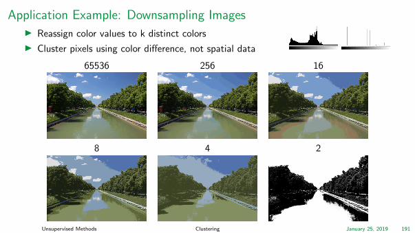
Application Example: Downsampling ImagesI Reassign color values to k distinct colors
I Cluster pixels using color difference, not spatial data
65536 256 16
8 4 2
Unsupervised Methods Clustering January 25, 2019 191

Major Clustering Approaches
I Partitioning algorithms: Find k partitions, minimizing someobjective function
I Probabilistic Model-Based Clustering (EM)
I Density-based: Find clusters based on connectivity and densityfunctions
I Hierarchical algorithms: Create a hierarchical decomposition ofthe set of objects
I Other methods:I Grid-basedI Neural networks (SOMs)I Graph-theoretical methodsI Subspace Clustering
Unsupervised Methods Clustering January 25, 2019 192
Agenda
1. Introduction
2. Basics
3. Unsupervised Methods3.1 Frequent Pattern Mining3.2 Clustering
3.2.1 Partitioning Methods3.2.2 Probabilistic Model-Based Methods3.2.3 Density-Based Methods3.2.4 Mean-Shift3.2.5 Spectral Clustering3.2.6 Hierarchical Methods3.2.7 Evaluation3.2.8 Ensemble Clustering
3.3 Outlier Detection
4. Supervised Methods
5. Advanced Topics

Partitioning Algorithms: Basic Concept
Partition
Given a set D, a partitioning C = C1, . . . ,Ck of D fulfils:
I Ci ⊆ D for all 1 ≤ i ≤ k
I Ci ∩ Cj = ∅ ⇐⇒ i 6= j
I⋃
Ci = D
(i.e. each element of D is in exactly one set Ci )
Goal
Construct a partitioning of a database D of n objects into a set of k (k ≤ n) clustersminimizing an objective function.
Exhaustively enumerating all possible partitionings into k sets in order to find theglobal minimum is too expensive.
Unsupervised Methods Clustering January 25, 2019 193

Partitioning Algorithms: Basic Concept
Popular Heuristic Methods
I Choose k representatives for clusters, e.g., randomlyI Improve these initial representatives iteratively:
I Assign each object to the cluster it “fits best” in the current clusteringI Compute new cluster representatives based on these assignmentsI Repeat until the change in the objective function from one iteration to the next
drops below a threshold
Example
I k-means: Each cluster is represented by the center of the cluster
I k-medoid: Each cluster is represented by one of its objects
Unsupervised Methods Clustering January 25, 2019 194

k-Means Clustering: Basic Idea
Idea1
Find a clustering such that thewithin-cluster variation of each cluster issmall and use the centroid of a cluster asrepresentative.
Objective
For a given k , form k groups so that thesum of the (squared) distances between themean of the groups and their elements isminimal
Poor clustering
μ
μ
μ
clustermeandistance
μ Centroids
Good clustering
μ
μ
μ
μ Centroids
1S.P. Lloyd: Least squares quantization in PCM. In IEEE Information Theory, 1982 (original version: technical report, Bell Labs, 1957)
Unsupervised Methods Clustering January 25, 2019 195

k-Means Clustering: Basic Notions
I Objects p = (p1, . . . , pd ) are points in a d-dimensional vector space (the mean µS
of a set of points S must be defined: µS = 1|S|∑
p∈S
p)
I Measure for the compactness of a cluster Cj (sum of squared distances):SSE (Cj ) =
∑p∈Cj
||p − µCj||22
I Measure for the compactness of a clustering C:SSE (C) =
∑Cj∈C
SSE (Cj ) =∑
p∈D
||p − µC(p)||22
I Optimal Partitioning: argminC
SSE (C)
I Optimizing the within-cluster variation is computationally challenging (NP-hard) use efficient heuristic algorithms
Unsupervised Methods Clustering January 25, 2019 196
k-Means Clustering: Algorithm
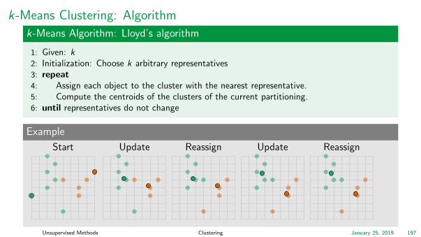
k-Means Algorithm: Lloyd’s algorithm
1: Given: k2: Initialization: Choose k arbitrary representatives3: repeat4: Assign each object to the cluster with the nearest representative.5: Compute the centroids of the clusters of the current partitioning.6: until representatives do not change
Example
Start Update Reassign Update Reassign
Unsupervised Methods Clustering January 25, 2019 197

k-Means: Voronoi Model for Convex Cluster Regions
Voronoi Diagram
I For a given set of points P = p1, . . . , pk (here: cluster representatives), aVoronoi diagram partitions the data space into Voronoi cells, one cell per point
I The cell of a point p ∈ P covers all points in the data space for which p is thenearest neighbors among the points from P
Observations
I The Voronoi cells of two neighboring pointspi , pj ∈ P are separated by the perpendicularhyperplane (”Mittelsenkrechte”) between pi and pj .
I Voronoi cells are intersections of half spaces and thusconvex regions
Unsupervised Methods Clustering January 25, 2019 198

k-Means: Discussion
Strength
I Relatively efficient: O(tkn) (n: #obj., k: #clus., t: #it.; typically: k, t n)
I Easy implementation
Weaknesses
I Applicable only when mean is defined
I Need to specify k , the number of clusters, in advance
I Sensitive to noisy data and outliers
I Clusters are forced to convex space partitions (Voronoi Cells)
I Result and runtime strongly depend on the initial partition; often terminates at alocal optimum – however: methods for a good initialization exist
Unsupervised Methods Clustering January 25, 2019 199

Variants: Basic Idea
One Problem of k-Means
Applicable only when mean is defined (vector space)
Alternatives for Mean representatives
I Median: (Artificial) Representative object ”in the middle”
I Mode: Value that appears most often
I Medoid: Representative object ”in the middle”
Objective
Find k representatives so that the sum of total distances (TD) between objects andtheir closest representative is minimal (more robust against outliers).
Unsupervised Methods Clustering January 25, 2019 200

k-Median
A B C D E F G H I J Ktiny
small
medium
large
huge
data point
median
Idea
I If there is an ordering on the data use median instead of mean.
I Compute median separately per dimension ( efficient computation)
Unsupervised Methods Clustering January 25, 2019 201

k-Mode
Technician Manager Cook Programmer Advisor
Cat
Dog
Snake
None
2
1
2
1
1
1 1 cdata point(count=c)
mode
Mode
I Given: categorical data D ⊆ Ω = A1× · · ·×Ad where Ai are categorical attributes
I A mode of D is a vector M = (m1, . . . ,md ) ∈ Ω that minimizesd(M,D) =
∑p∈D d(p,M) where d is a distance function for categorical values
(e.g. Hamming distance)
I Note: M is not necessarily an element of D
Unsupervised Methods Clustering January 25, 2019 202

k-Mode
Theorem to determine a mode
Let f (c , j ,D) = 1n |p ∈ D | p[j ] = c| be the relative frequency of category c of
attribute Aj in the data, then:
d(M,D) is minimal ⇔ ∀j ∈ 1, . . . , d∀c ∈ Aj : f (mj , j ,D) ≥ f (c , j ,D)
I This allows to use the k-Means paradigm to cluster categorical data withoutlosing its efficiency
I k-Modes algorithm1 proceeds similar to k-Means algorithm
I Note: The mode of a dataset might be not unique
1Huang, Z. ”A Fast Clustering Algorithm to Cluster very Large Categorical Data Sets in Data Mining” DMKD (1997)
Unsupervised Methods Clustering January 25, 2019 203

k-Medoid
Potential problems with previous methods:
I Artificial centroid object might not make sense (e.g. education=”high school”and occupation=”professor”)
I There might only be a distance function available but no explicit attribute-baseddata representations (e.g. Edit Distance on strings)
Partitioning Around Medoids 1: Initialization
Given k, the k-medoid algorithm is initialized as follows:
I Select k objects arbitrarily as initial medoids (representatives)
I Assign each remaining (non-medoid) object to the cluster with the nearestrepresentative
I Compute current TDcurrent
1Kaufman, Leonard, and Peter Rousseeuw. ”Clustering by means of medoids.” (1987)
Unsupervised Methods Clustering January 25, 2019 204

k-Medoid
Partitioning Around Medoids (PAM) Algorithm
procedure PAM(Set D, Integer k)Initialize k medoids∆TD = −∞while ∆TD < 0 do
Compute TDN↔M for each pair (medoid M, non-medoid N), i.e., TD after swapping M with NChoose pair (M,N) with minimal ∆TD = TDN↔M − TDcurrent
if ∆TD < 0 thenReplace medoid M with non-medoid NTDcurrent ← TDN↔M
Store current medoids and assignments as best partitioning so farreturn medoids
I Problem with PAM: high complexity O(tk(n − k)2
)I Several heuristics can be employed, e.g. CLARANS 1: randomly select (medoid,
non-medoid)-pairs instead of considering all pairs
1Ng, Raymond T., and Jiawei Han. ”CLARANS: A method for clustering objects for spatial data mining.” IEEE TKDE (2002)
Unsupervised Methods Clustering January 25, 2019 205

K -Means/Median/Mode/Medoid Clustering: Discussion
k-Means k-Median k-Mode k-Medoid
data numerical (mean) ordinal categorical metric
efficiency high O (tkn) low O(tk(n − k)2
)sensitivityto outliers
high low
I Strength: Easy implementation (many variations and optimizations exist)I Weaknesses
I Need to specify k in advanceI Clusters are forced to convex space partitions (Voronoi Cells)I Result and runtime strongly depend on the initial partition; often terminates at a
local optimum – however: methods for good initialization exist
Unsupervised Methods Clustering January 25, 2019 206

Initialization of Partitioning Clustering Methods
I NaiveI Choose sample A of the datasetI Cluster A and use centers as initialization
I k-means++1
I Select first center uniformly at randomI Choose next point with probability proportional to the
squared distance to the nearest center already chosenI Repeat until k centers have been selectedI Guarantees an approximation ratio of O(log k) (standard
k-means can generate arbitrarily bad clusterings)
I In general: Repeat with different initial centers andchoose result with lowest clustering error
Bad initialization
Good initialization
1Arthur, D., Vassilvitskii, S. ”k-means++: The Advantages of Careful Seeding.” ACM-SIAM Symposium on Discrete Algorithms (2007)
Unsupervised Methods Clustering January 25, 2019 207

Choice of the Parameter k
I Idea for a method:I Determine a clustering for each k = 2, . . . , n − 1I Choose the ”best” clustering
I But how to measure the quality of a clustering?I A measure should not be monotonic over kI The measures for the compactness of a clustering SSE and TD are monotonously
decreasing with increasing value of k .
Silhouette-Coefficient 1
Quality measure for k-means or k-medoid clusterings that is not monotonic over k.
1Rousseeuw, P. ”Silhouettes: A Graphical Aid to the Interpretation and Validation of Cluster Analysis”. Computational and Applied
Mathematics (1987)
Unsupervised Methods Clustering January 25, 2019 208

The Silhouette Coefficient
Basic idea
I How good is the clustering = how appropriate is the mapping of objects to clustersI Elements in cluster should be ”similar” to their representative
I Measure the average distance of objects to their representative: a(o)
I Elements in different clusters should be ”dissimilar”I Measure the average distance of objects to alternative clusters (i.e. second closest
cluster): b(o)
Unsupervised Methods Clustering January 25, 2019 209

The Silhouette Coefficient
I a(o) = ”Avg. distance between o and objectsin its cluster A.”
a(o) =1
|C (o)|∑
p∈C(o)
d(o, p)
I b(o): ”Smallest avg. distance between o andobjects in other cluster.”
b(o) = minCi 6=C(o)
1
|Ci |∑p∈Ci
d(o, p)
Unsupervised Methods Clustering January 25, 2019 210
The Silhouette Coefficient
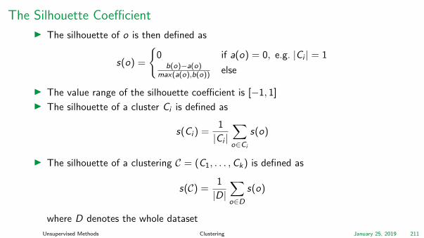
I The silhouette of o is then defined as
s(o) =
0 if a(o) = 0, e.g. |Ci | = 1
b(o)−a(o)max(a(o),b(o)) else
I The value range of the silhouette coefficient is [−1, 1]
I The silhouette of a cluster Ci is defined as
s(Ci ) =1
|Ci |∑o∈Ci
s(o)
I The silhouette of a clustering C = (C1, . . . ,Ck ) is defined as
s(C) =1
|D|∑o∈D
s(o)
where D denotes the whole dataset
Unsupervised Methods Clustering January 25, 2019 211
The Silhouette Coefficient
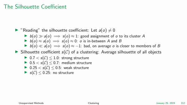
I ”Reading” the silhouette coefficient: Let a(o) 6= 0I b(o) a(o) =⇒ s(o) ≈ 1: good assignment of o to its cluster AI b(o) ≈ a(o) =⇒ s(o) ≈ 0: o is in-between A and BI b(o) a(o) =⇒ s(o) ≈ −1: bad, on average o is closer to members of B
I Silhouette coefficient s(C) of a clustering: Average silhouette of all objectsI 0.7 < s(C) ≤ 1.0: strong structureI 0.5 < s(C) ≤ 0.7: medium structureI 0.25 < s(C) ≤ 0.5: weak structureI s(C) ≤ 0.25: no structure
Unsupervised Methods Clustering January 25, 2019 212

Silhouette Coefficient: Example
dataset with 10 clusters
Image from Tan, Steinbach, Kumar: Introduction to Data Mining (Pearson, 2006)Unsupervised Methods Clustering January 25, 2019 213
Agenda
1. Introduction
2. Basics
3. Unsupervised Methods3.1 Frequent Pattern Mining3.2 Clustering
3.2.1 Partitioning Methods3.2.2 Probabilistic Model-Based Methods3.2.3 Density-Based Methods3.2.4 Mean-Shift3.2.5 Spectral Clustering3.2.6 Hierarchical Methods3.2.7 Evaluation3.2.8 Ensemble Clustering
3.3 Outlier Detection
4. Supervised Methods
5. Advanced Topics

Expectation Maximization (EM)
I Statistical approach for finding maximum likelihoodestimates of parameters in probabilistic models.
I Here: Using EM as clustering algorithm
I Approach: Observations are drawn from one of severalcomponents of a mixture distribution.
I Main idea:I Define clusters as probability distributions → each
object has a certain probability of belonging to eachcluster
I Iteratively improve the parameters of each distribution(e.g. center, ”width” and ”height” of a Gaussiandistribution) until some quality threshold is reached
↓
↓
Additional Literature: C. M. Bishop ”Pattern Recognition and Machine Learning”, Springer, 2009Unsupervised Methods Clustering January 25, 2019 214
Excursus: Gaussian Mixture Distributions
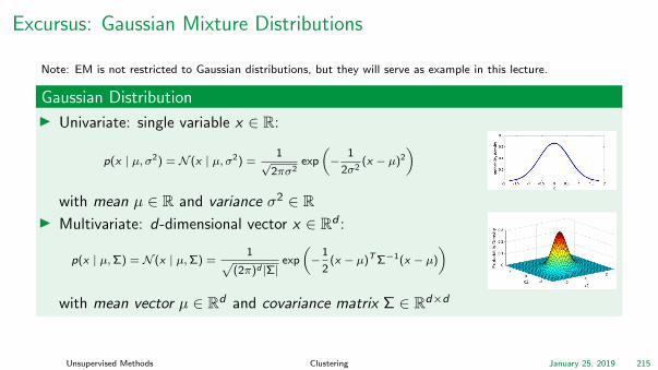
Note: EM is not restricted to Gaussian distributions, but they will serve as example in this lecture.
Gaussian Distribution
I Univariate: single variable x ∈ R:
p(x | µ, σ2) = N (x | µ, σ2) =1
√2πσ2
exp
(−
1
2σ2(x − µ)2
)
with mean µ ∈ R and variance σ2 ∈ RI Multivariate: d-dimensional vector x ∈ Rd :
p(x | µ,Σ) = N (x | µ,Σ) =1√
(2π)d |Σ|exp
(−
1
2(x − µ)T Σ−1(x − µ)
)
with mean vector µ ∈ Rd and covariance matrix Σ ∈ Rd×d
Unsupervised Methods Clustering January 25, 2019 215
Excursus: Gaussian Mixture Distributions
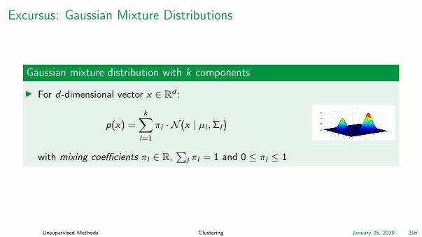
Gaussian mixture distribution with k components
I For d-dimensional vector x ∈ Rd :
p(x) =k∑
l=1
πl · N (x | µl ,Σl )
with mixing coefficients πl ∈ R,∑
l πl = 1 and 0 ≤ πl ≤ 1
Unsupervised Methods Clustering January 25, 2019 216

EM: Exemplary Application
Example taken from: C. M. Bishop ”Pattern Recognition and Machine Learning”, 2009Unsupervised Methods Clustering January 25, 2019 217
EM: Clustering Model
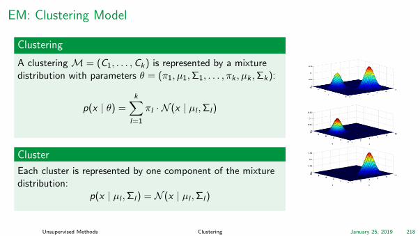
Clustering
A clustering M = (C1, . . . ,Ck ) is represented by a mixturedistribution with parameters θ = (π1, µ1,Σ1, . . . , πk , µk ,Σk ):
p(x | θ) =k∑
l=1
πl · N (x | µl ,Σl )
Cluster
Each cluster is represented by one component of the mixturedistribution:
p(x | µl ,Σl ) = N (x | µl ,Σl )
Unsupervised Methods Clustering January 25, 2019 218
EM: Maximum Likelihood Estimation
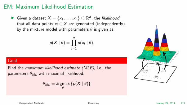
I Given a dataset X = x1, . . . , xn ⊆ Rd , the likelihoodthat all data points xi ∈ X are generated (independently)by the mixture model with parameters θ is given as:
p(X | θ) =n∏
i=1
p(xi | θ)
Goal
Find the maximum likelihood estimate (MLE), i.e., theparameters θML with maximal likelihood:
θML = argmaxθp(X | θ)
Unsupervised Methods Clustering January 25, 2019 219
EM: Maximum Likelihood Estimation
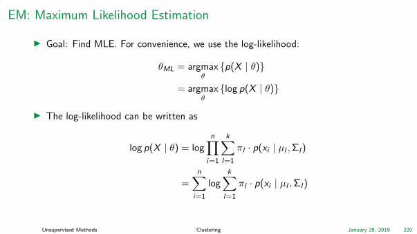
I Goal: Find MLE. For convenience, we use the log-likelihood:
θML = argmaxθp(X | θ)
= argmaxθlog p(X | θ)
I The log-likelihood can be written as
log p(X | θ) = logn∏
i=1
k∑l=1
πl · p(xi | µl ,Σl )
=n∑
i=1
logk∑
l=1
πl · p(xi | µl ,Σl )
Unsupervised Methods Clustering January 25, 2019 220

EM: Maximum Likelihood Estimation
I Maximization w.r.t. the means:
∂ log p(X | θ)
∂µj=
n∑i=1
∂ log p(xi | θ)
∂µj=
n∑i=1
∂ log p(xi |θ)∂µj
p(xi | θ)=
n∑i=1
∂ log p(xi |θ)∂µj∑k
l=1 p(xi | µl ,Σl )
=n∑
i=1
πj · Σ−1j (xi − µj ) · N (xi | µj ,Σj )∑k
l=1 p(xi | µl ,Σl )
= Σ−1j
n∑i=1
(xi − µj )πj · N (xi | µj ,Σj )∑kl=1 πl · N (xi | µl ,Σl )
!= 0
I Use ∂∂µjN (xi | µj ,Σj ) = Σ−1
j (xi − µj ) · N (xi | µj ,Σj )
I Define γj (xi ) := πj · N (xi | µj ,Σj ): Probability that component j generated xi
Unsupervised Methods Clustering January 25, 2019 221

EM: Maximum Likelihood Estimation
I Maximization w.r.t. the means yields
µj =
∑ni=1 γj (xi )xi∑n
i=1 γj (xi )
I Maximization w.r.t. the covariance matrices yields
Σj =
∑ni=1 γj (xi )(xi − µj )(xi − µj )
T∑ni=1 γj (xi )
I Maximization w.r.t. the mixing coefficients yields
πj =
∑ni=1 γj (xi )∑k
l=1
∑ni=1 γl (xi )
Unsupervised Methods Clustering January 25, 2019 222
EM: Maximum Likelihood Estimation
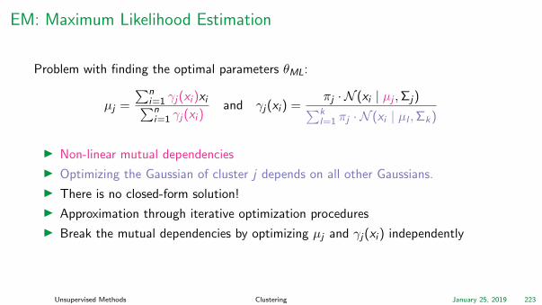
Problem with finding the optimal parameters θML:
µj =
∑ni=1 γj (xi )xi∑n
i=1 γj (xi )and γj (xi ) =
πj · N (xi | µj ,Σj )∑kl=1 πj · N (xi | µl ,Σk )
I Non-linear mutual dependencies
I Optimizing the Gaussian of cluster j depends on all other Gaussians.
I There is no closed-form solution!
I Approximation through iterative optimization procedures
I Break the mutual dependencies by optimizing µj and γj (xi ) independently
Unsupervised Methods Clustering January 25, 2019 223

EM: Iterative Optimization
Iterative Optimization
1. Initialize means µj , covariances Σj , and mixing coefficients πj and evaluate theinitial log-likelihood.
2. E-step: Evaluate the responsibilities using the current parameter values:
γnewj (xi ) =
πj · N (xi | µj ,Σj )∑kl=1 πj · N (xi | µl ,Σl )
3. M-step: Re-estimate the parameters using the current responsibilities:
µnewj =
∑ni=1 γ
newj (xi )xi∑n
i=1 γnewj (xi )
...
Unsupervised Methods Clustering January 25, 2019 224
EM: Iterative Optimization
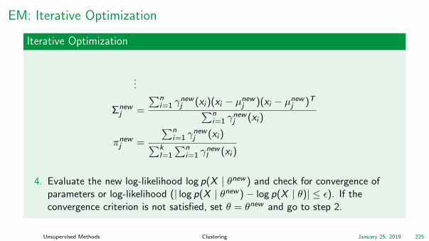
Iterative Optimization
...
Σnewj =
∑ni=1 γ
newj (xi )(xi − µnew
j )(xi − µnewj )T∑n
i=1 γnewj (xi )
πnewj =
∑ni=1 γ
newj (xi )∑k
l=1
∑ni=1 γ
newl (xi )
4. Evaluate the new log-likelihood log p(X | θnew ) and check for convergence ofparameters or log-likelihood (| log p(X | θnew )− log p(X | θ)| ≤ ε). If theconvergence criterion is not satisfied, set θ = θnew and go to step 2.
Unsupervised Methods Clustering January 25, 2019 225

EM: Turning the Soft Clustering into a Partitioning
I EM obtains a soft clustering (each object belongs to each cluster with a certainprobability) reflecting the uncertainty of the most appropriate assignment
I Modification to obtain a partitioning variant: Assign each object to the cluster towhich it belongs with the highest probability
C (xi ) = argmaxl∈1,...,k
γl (xi )
Example taken from: C. M. Bishop ”Pattern Recognition and Machine Learning”, 2009Unsupervised Methods Clustering January 25, 2019 226

EM: Discussion
I Superior to k-Means for clusters of varying size or clustershaving differing variancesI More accurate data representation
I Convergence to (possibly local) maximumI Computational effort for t iterations: O(tnk)
I t is quite high in many cases
I Both, result and runtime, strongly depend onI the initial assignment
I Do multiple random starts and choose the final estimatewith highest likelihood
I Initialize with clustering algorithms (e.g., k-Means): usuallyconverges much faster
I Local maxima and initialization issues have been addressedin various extensions of EM
I a proper choice of k (next slide)
Unsupervised Methods Clustering January 25, 2019 227

EM: Model Selection for Determining Parameter k
Problem
Classical trade-off problem for selecting the proper number of components k :
I If k is too high, the mixture may overfit the data
I If k is too low, the mixture may not be flexible enough to approximate the data
Idea
Determine candidate models θk for k ∈ kmin, . . . , kmax and select the modelaccording to some quality measure qual :
θk∗ = maxk∈kmin,...,kmax
qual(θk )
I Silhouette Coefficient (as for k-Means) only works for partitioning approaches
I The likelihood is nondecreasing in k
Unsupervised Methods Clustering January 25, 2019 228

EM: Model Selection for Determining Parameter k
Solution
Deterministic or stochastic model selection methods 1 which try to balance thegoodness of fit with simplicity.
I Deterministic:qual(θk ) = log p(X | θk ) + P(k)
where P(k) is an increasing function penalizing higher values of k
I Stochastic: Based on Markov Chain Monte Carlo (MCMC)
1G. McLachlan and D. Peel. Finite Mixture Models. Wiley, New York, 2000.Unsupervised Methods Clustering January 25, 2019 229
Agenda
1. Introduction
2. Basics
3. Unsupervised Methods3.1 Frequent Pattern Mining3.2 Clustering
3.2.1 Partitioning Methods3.2.2 Probabilistic Model-Based Methods3.2.3 Density-Based Methods3.2.4 Mean-Shift3.2.5 Spectral Clustering3.2.6 Hierarchical Methods3.2.7 Evaluation3.2.8 Ensemble Clustering
3.3 Outlier Detection
4. Supervised Methods
5. Advanced Topics

Density-Based Clustering
Basic Idea
Clusters are dense regions in the data space,separated by regions of lower density
Results of a k-medoid algorithm for k = 4:
Unsupervised Methods Clustering January 25, 2019 230

Density-Based Clustering: Basic Concept
Note
Different density-based approaches exist in the literature. Here we discuss the ideasunderlying the DBSCAN algorithm.
Intuition for Formalization
I For any point in a cluster, the local point density around that point has to exceedsome threshold
I The set of points from one cluster is spatially connected
Unsupervised Methods Clustering January 25, 2019 231

Density-Based Clustering: Basic Concept
Local Point Density
Local point density at a point q defined by two parameters:
I ε-radius for the neighborhood of point q
Nε(q) = p ∈ D | dist(p, q) ≤ ε (1)
In this chapter, we assume that q ∈ Nε(q)!
I MinPts: minimum number of points in the given neighbourhood Nε(q).
Unsupervised Methods Clustering January 25, 2019 232

Density-Based Clustering: Basic Concept
q
Core Point
q is called a core object (or core point) w.r.t. ε, MinPts if |Nε(q)| ≥ minPts
Unsupervised Methods Clustering January 25, 2019 233

Density-Based Clustering: Basic Definitions
p
q
p
q
(Directly) Density-Reachable
p directly density-reachable from q w.r.t. ε, MinPts if:
1. p ∈ Nε(q) and
2. q is core object w.r.t. ε,MinPts
Density-reachable is the transitive closure of directly density-reachable
Unsupervised Methods Clustering January 25, 2019 234

Density-Based Clustering: Basic Definitions
p
qo
Density-Connected
p is density-connected to a point q w.r.t. ε, MinPts if there is a point o such thatboth, p and q are density-reachable from o w.r.t. ε,MinPts
Unsupervised Methods Clustering January 25, 2019 235

Density-Based Clustering: Basic Definitions
Density-Based Cluster
∅ ⊂ C ⊆ D with database D satisfying:
Maximality: If q ∈ C and p is density-reachable from q then p ∈ CConnectivity: Each object in C is density-connected to all other objects in C
Unsupervised Methods Clustering January 25, 2019 236
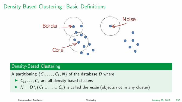
Density-Based Clustering: Basic Definitions
Core
BorderNoise
Density-Based Clustering
A partitioning C1, . . . ,Ck ,N of the database D where
I C1, . . . ,Ck are all density-based clusters
I N = D \ (C1 ∪ . . . ∪ Ck ) is called the noise (objects not in any cluster)
Unsupervised Methods Clustering January 25, 2019 237

Density-Based Clustering: DBSCAN Algorithm
Basic Theorem
I Each object in a density-based cluster C is density-reachable from any of itscore-objects
I Nothing else is density-reachable from core objects.
Unsupervised Methods Clustering January 25, 2019 238
Density-Based Clustering: DBSCAN Algorithm
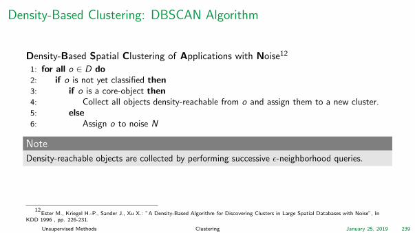
Density-Based Spatial Clustering of Applications with Noise12
1: for all o ∈ D do2: if o is not yet classified then3: if o is a core-object then4: Collect all objects density-reachable from o and assign them to a new cluster.5: else6: Assign o to noise N
Note
Density-reachable objects are collected by performing successive ε-neighborhood queries.
12Ester M., Kriegel H.-P., Sander J., Xu X.: ”A Density-Based Algorithm for Discovering Clusters in Large Spatial Databases with Noise”, In
KDD 1996 , pp. 226-231.
Unsupervised Methods Clustering January 25, 2019 239
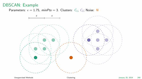
DBSCAN: ExampleParameters: ε = 1.75, minPts = 3. Clusters: C1, C2; Noise: N
ε ε
Unsupervised Methods Clustering January 25, 2019 240

Determining the Parameters ε and MinPts
Recap
Cluster: Point density higher than specified by ε and MinPts
Idea
Use the point density of the least dense cluster in the data set as parameters.
Problem
How to determine this?
Unsupervised Methods Clustering January 25, 2019 241

Determining the Parameters ε and MinPts
Heuristic
1. Fix a value for MinPts (default: 2d − 1 where d is thedimension of the data space)
2. Compute the k-distance for all points p ∈ D (distancefrom p to the its k-nearest neighbor), with k = minPts.
3. Create a k-distance plot, showing the k-distances of allobjects, sorted in decreasing order
4. The user selects ”border object” o from theMinPts-distance plot: ε is set to MinPts-distance(o).
3-d
ista
nce
"border object"
Objects
first "kink"
Unsupervised Methods Clustering January 25, 2019 242

Determining the Parameters ε and MinPts: Problematic Example
A
B
C
D
E
D
F
G
D1D2
G1
G2G3
A
B
C
EF
G1
G2
D2D1
D
G
G3
A, B, C
B
B, D, E
Objects
A,B,C
B,D,E
D1,D2,G1,G2,G3
D,F,G
Unsupervised Methods Clustering January 25, 2019 243

Database Support for Density-Based Clustering
Standard DBSCAN evaluation is based on recursive database traversal. Bohm et al.13
observed that DBSCAN, among other clustering algorithms, may be efficiently built ontop of similarity join operations.
ε-Similarity Join
An ε-similarity join yields all pairs of ε-similar objects from two data sets Q, P:
Q ./ε P = (q, p) ∈ Q × P | dist(q, p) ≤ ε
SQL Query
SELECT ∗ FROM Q,P WHERE dist(Q,P) ≤ ε
13Bohm C., Braunmuller, B., Breunig M., Kriegel H.-P.: High performance clustering based on the similarity join. CIKM 2000: 298-305.
Unsupervised Methods Clustering January 25, 2019 244

Database Support for Density-Based Clustering
ε-Similarity Self-Join
An ε-similarity self join yields all pairs of ε-similar objects from a database D.
D ./ε D = (q, p) ∈ D × D | dist(q, p) ≤ ε
SQL Query
SELECT ∗ FROM D q,D p WHERE dist(q, p) ≤ ε
Unsupervised Methods Clustering January 25, 2019 245
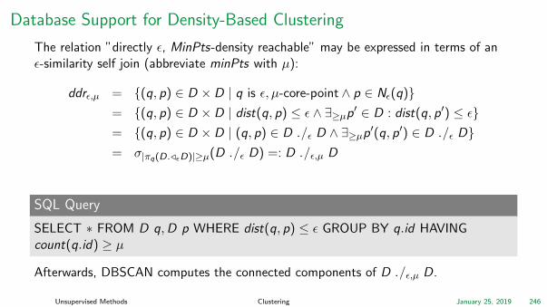
Database Support for Density-Based Clustering
The relation ”directly ε, MinPts-density reachable” may be expressed in terms of anε-similarity self join (abbreviate minPts with µ):
ddrε,µ = (q, p) ∈ D × D | q is ε, µ-core-point ∧ p ∈ Nε(q)= (q, p) ∈ D × D | dist(q, p) ≤ ε ∧ ∃≥µp′ ∈ D : dist(q, p′) ≤ ε= (q, p) ∈ D × D | (q, p) ∈ D ./ε D ∧ ∃≥µp′(q, p′) ∈ D ./ε D= σ|πq(D./εD)|≥µ(D ./ε D) =: D ./ε,µ D
SQL Query
SELECT ∗ FROM D q,D p WHERE dist(q, p) ≤ ε GROUP BY q.id HAVINGcount(q.id) ≥ µ
Afterwards, DBSCAN computes the connected components of D ./ε,µ D.
Unsupervised Methods Clustering January 25, 2019 246
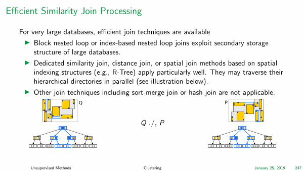
Efficient Similarity Join Processing
For very large databases, efficient join techniques are available
I Block nested loop or index-based nested loop joins exploit secondary storagestructure of large databases.
I Dedicated similarity join, distance join, or spatial join methods based on spatialindexing structures (e.g., R-Tree) apply particularly well. They may traverse theirhierarchical directories in parallel (see illustration below).
I Other join techniques including sort-merge join or hash join are not applicable.
Q
Q ./ε P
P
Unsupervised Methods Clustering January 25, 2019 247

DBSCAN: Discussion
Advantages
I Clusters can have arbitrary shape and size; no restriction to convex shapes
I Number of clusters is determined automatically
I Can separate clusters from surrounding noise
I Complexity: Nε-query: O(n), DBSCAN: O(n2).
I Can be supported by spatial index structures ( Nε-query: O(log n))
Disadvantages
I Input parameters may be difficult to determine
I In some situations very sensitive to input parameter setting
Unsupervised Methods Clustering January 25, 2019 248
Agenda
1. Introduction
2. Basics
3. Unsupervised Methods3.1 Frequent Pattern Mining3.2 Clustering
3.2.1 Partitioning Methods3.2.2 Probabilistic Model-Based Methods3.2.3 Density-Based Methods3.2.4 Mean-Shift3.2.5 Spectral Clustering3.2.6 Hierarchical Methods3.2.7 Evaluation3.2.8 Ensemble Clustering
3.3 Outlier Detection
4. Supervised Methods
5. Advanced Topics
Iterative Mode Search
Idea
Find modes in the point density.
Algorithm14
1. Select a window size ε, starting position m
2. Calculate the mean of all points inside the window W (m).
3. Shift the window to that position
4. Repeat until convergence.
14K. Fukunaga, L. Hostetler: The Estimation of the Gradient of a Density Function, with Applications in Pattern Recognition, IEEE Trans
Information Theory, 1975
Unsupervised Methods Clustering January 25, 2019 249

Iterative Mode Search: Example
Unsupervised Methods Clustering January 25, 2019 250

Mean Shift: Core Algorithm
Algorithm15
Apply iterative mode search for each data point. Group those that converge to thesame mode (called Basin of Attraction).
15D. Comaniciu, P. Meer. Mean shift: A robust approach toward feature space analysis. IEEE Trans. on pattern analysis and machine
intelligence, 2002
Unsupervised Methods Clustering January 25, 2019 251

Mean Shift: Extensions
Weighted Mean
Use different weights for the points in the window calculated by some kernel κ
m(i+1) =
∑x∈W (m(i))
κ(x)x∑x∈W (m(i))
κ(x)
Binning
First quantise data points to grid. Apply iterative mode seeking only once per bin.
Unsupervised Methods Clustering January 25, 2019 252

Mean Shift: Discussion
Disadvantages
I Relatively high complexity: Nε-query (=windowing): O(n). Algorithm: O(tn2)
Advantages
I Clusters can have arbitrary shape and size; no restriction to convex shapes
I Number of clusters is determined automatically
I Robust to outliers
I Easy implementation and parallelisation
I Single parameter: ε
I Support by spatial index: Nε-query (=windowing): O(log n). Algorithm:O(tn log n)
Unsupervised Methods Clustering January 25, 2019 253

Agenda
1. Introduction
2. Basics
3. Unsupervised Methods3.1 Frequent Pattern Mining3.2 Clustering
3.2.1 Partitioning Methods3.2.2 Probabilistic Model-Based Methods3.2.3 Density-Based Methods3.2.4 Mean-Shift3.2.5 Spectral Clustering3.2.6 Hierarchical Methods3.2.7 Evaluation3.2.8 Ensemble Clustering
3.3 Outlier Detection
4. Supervised Methods
5. Advanced Topics

Clustering as Graph Partitioning
Approach
I Data is modeled by a similarity graph G = (V ,E )I Vertices v ∈ V : Data objectsI Weighted edges vi , vj ∈ E : Similarity of vi and vj
I Common variants: ε-neighborhood graph, k-nearestneighbor graph, fully connected graph
I Cluster the data by partitioning the similarity graphI Idea: Find global minimum cut
I Only considers inter-cluster edges, tends to cut smallvertex sets from the graph
I Partitions graph into two clusters
I Instead, we want a balanced multi-way partitioningI Such problems are NP-hard, use approximations
Unsupervised Methods Clustering January 25, 2019 254

Spectral Clustering
Given
Undirected graph G with weighted edges
I Let W be the (weighted) adjacency matrix of the graph
I And D its degree matrix with Dii =∑n
j=1 Wij ; otherentries are 0
Aim
Partition G into k subsets, minimizing a function of the edgeweights between/within the partitions.
Unsupervised Methods Clustering January 25, 2019 255
Spectral Clustering
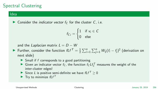
Idea
I Consider the indicator vector fC for the cluster C , i.e.
fC i =
1 if vi ∈ C
0 else
and the Laplacian matrix L = D −WI Further, consider the function fLf T = 1
2
∑ni=1
∑nj=1 Wij (fi − fj )
2 (derivation on
next slide)I Small if f corresponds to a good partitioningI Given an indicator vector fC , the function fC Lf T
C measures the weight of theinter-cluster edges!
I Since L is positive semi-definite we have fLf T ≥ 0I Try to minimize fLf T
Unsupervised Methods Clustering January 25, 2019 256

Spectral Clustering
fLf T = fDf T − fWf T
=∑
i
di f2
i −∑
ij
wij fi fj
=1
2
∑i
(∑
j
wij )f 2i − 2
∑ij
wij fi fj +∑
j
(∑
i
wij )f 2j
=
1
2
∑ij
wij f2
i − 2∑
ij
wij fi fj +∑
ij
wij f2
j
=
1
2
∑ij
wij (f 2i − 2fi fj + f 2
j )
=1
2
∑ij
wij (fi − fj )2
Unsupervised Methods Clustering January 25, 2019 257
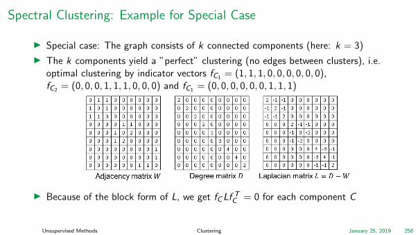
Spectral Clustering: Example for Special Case
I Special case: The graph consists of k connected components (here: k = 3)
I The k components yield a ”perfect” clustering (no edges between clusters), i.e.optimal clustering by indicator vectors fC1 = (1, 1, 1, 0, 0, 0, 0, 0, 0),fC2 = (0, 0, 0, 1, 1, 1, 0, 0, 0) and fC1 = (0, 0, 0, 0, 0, 0, 1, 1, 1)
I Because of the block form of L, we get fC Lf TC = 0 for each component C
Unsupervised Methods Clustering January 25, 2019 258

Connected Components and Eigenvectors
I General goal: find indicator vectors minimizing function fLf T besides the trivialindicator vector fC = (1, . . . , 1)
I Problem: Finding solution is NP-hard (cf. graph cut problems)
I How can we relax the problem to find a (good) solution more efficiently?I Observation: For the special case with k connected components, the k indicator
vectors fulfilling fC Lf TC = 0 yield the perfect clustering
I The indicator vector for each component is an eigenvector of L with eigenvalue 0I The k indicator vectors are orthogonal to each other (linearly independent)
Lemma
The number of linearly independent eigenvectors with eigenvalue 0 for L equals thenumber of connected components in the graph.
Unsupervised Methods Clustering January 25, 2019 259

Spectral Clustering: General CaseI In general: L does not have zero-eigenvectors
I One large connected component, no perfect clusteringI Determine the (linear independent) eigenvectors with
the k smallest eigenvalues!
I Example: The 3 clusters are now connected byadditional edges
I Smallest eigenvalues of L: (0.23, 0.70, 3.43)
Eigenvectors of L
Unsupervised Methods Clustering January 25, 2019 260

Spectral Clustering: Data TransformationI How to find the clusters based on the eigenvectors?
I Easy in special setting: 0-1 values; now: arbitrary real numbersI Data transformation: Represent each vertex by a vector of its corresponding
components in the eigenvectorsI In the special case, the representations of vertices from the same connected
component are equal, e.g. v1, v2, v3 are transformed to (1, 0, 0)I In general case only similar eigenvector representations
I Clustering (e.g. k-Means) on transformed data points yields final result
Unsupervised Methods Clustering January 25, 2019 261

Illustration: Embedding of Vertices to a Vector Space
Spectral layout of previous example
Unsupervised Methods Clustering January 25, 2019 262

Spectral Clustering: Discussion
Advantages
I No assumptions on the shape of the clustersI Easy to implement
Disadvantages
I May be sensitive to construction of the similarity graphI Runtime: k smallest eigenvectors can be computed in O(n3) (worst case)
I However: Much faster on sparse graphs, faster variants have been developed
I Several variations of spectral clustering exist, using different Laplacian matriceswhich can be related to different graph cut problems 1
1Von Luxburg, U.: A tutorial on spectral clustering, in Statistics and Computing, 2007
Unsupervised Methods Clustering January 25, 2019 263

Agenda
1. Introduction
2. Basics
3. Unsupervised Methods3.1 Frequent Pattern Mining3.2 Clustering
3.2.1 Partitioning Methods3.2.2 Probabilistic Model-Based Methods3.2.3 Density-Based Methods3.2.4 Mean-Shift3.2.5 Spectral Clustering3.2.6 Hierarchical Methods3.2.7 Evaluation3.2.8 Ensemble Clustering
3.3 Outlier Detection
4. Supervised Methods
5. Advanced Topics

From Partitioning to Hierarchical Clustering
Global parameters to separate all clusters with a partitioning clustering method maynot exist:
Need a hierarchical clustering algorithm in these situations
Unsupervised Methods Clustering January 25, 2019 264
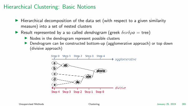
Hierarchical Clustering: Basic Notions
I Hierarchical decomposition of the data set (with respect to a given similaritymeasure) into a set of nested clusters
I Result represented by a so called dendrogram (greek δενδρo = tree)I Nodes in the dendrogram represent possible clustersI Dendrogram can be constructed bottom-up (agglomerative approach) or top down
(divisive approach)
Unsupervised Methods Clustering January 25, 2019 265
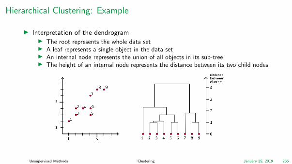
Hierarchical Clustering: Example
I Interpretation of the dendrogramI The root represents the whole data setI A leaf represents a single object in the data setI An internal node represents the union of all objects in its sub-treeI The height of an internal node represents the distance between its two child nodes
Unsupervised Methods Clustering January 25, 2019 266
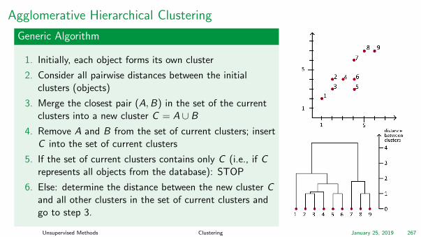
Agglomerative Hierarchical Clustering
Generic Algorithm
1. Initially, each object forms its own cluster
2. Consider all pairwise distances between the initialclusters (objects)
3. Merge the closest pair (A,B) in the set of the currentclusters into a new cluster C = A ∪ B
4. Remove A and B from the set of current clusters; insertC into the set of current clusters
5. If the set of current clusters contains only C (i.e., if Crepresents all objects from the database): STOP
6. Else: determine the distance between the new cluster Cand all other clusters in the set of current clusters andgo to step 3.
Unsupervised Methods Clustering January 25, 2019 267

Single-Link Method and Variants
I Agglomerative hierarchical clustering requires a distance function for clusters
I Given: a distance function dist(p, q) for database objects
I The following distance functions for clusters (i.e., sets of objects) X and Y arecommonly used for hierarchical clustering:
Single-Link: distsl (X ,Y ) = minx∈X ,y∈Y dist(x , y)Complete-Link: distcl (X ,Y ) = maxx∈X ,y∈Y dist(x , y)Average-Link: distal (X ,Y ) = 1
|X |·|Y |∑
x∈X ,y∈Y dist(x , y)
Unsupervised Methods Clustering January 25, 2019 268

Divisive Hierarchical Clustering
General Approach: Top Down
I Initially, all objects form one clusterI Repeat until all clusters are singletons
I Choose a cluster to split → how?I Replace the chosen cluster with the sub-clusters and split into two → how to split?
Example solution: DIANA
I Select the cluster C with largest diameter for splittingI Search the most disparate object o in C (highest average dissimilarity)
I Splinter group S = oI Iteratively assign the o′ /∈ S with the highest D(o′) > 0 to the splinter group until
D(o′) ≤ 0 for all o′ /∈ S , where
D(o′) =∑
oj∈C\S
d(o′, oj )
|C \ S |−∑oi∈S
d(o′, oi )
|S |
Unsupervised Methods Clustering January 25, 2019 269

Discussion Agglomerative vs. Divisive HC
I Divisive and Agglomerative HC need n − 1 stepsI Agglomerative HC has to consider n(n−1)
2 =(
n2
)combinations in the first step
I Divisive HC potentially has 2n−1 − 1 many possibilities to split the data in its firststep. Not every possibility has to be considered (DIANA)
I Divisive HC is conceptually more complex since it needs a second ”flat” clusteringalgorithm (splitting procedure)
I Agglomerative HC decides based on local patterns
I Divisive HC uses complete information about the global data distribution ableto provide better clusterings than Agglomerative HC?
Unsupervised Methods Clustering January 25, 2019 270
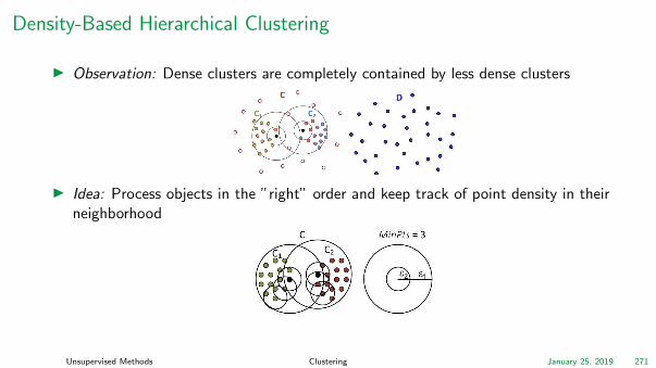
Density-Based Hierarchical Clustering
I Observation: Dense clusters are completely contained by less dense clusters
I Idea: Process objects in the ”right” order and keep track of point density in theirneighborhood
Unsupervised Methods Clustering January 25, 2019 271
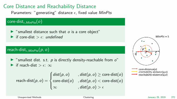
Core Distance and Reachability DistanceParameters: ”generating” distance ε, fixed value MinPts
core-distε,MinPts(o)
I ”smallest distance such that o is a core object”I if core-dist > ε: undefined
reach-distε,MinPts(p, o)
I ”smallest dist. s.t. p is directly density-reachable from o”I if reach-dist > ε: ∞
reach-dist(p, o) =
dist(p, o) , dist(p, o) ≥ core-dist(o)
core-dist(o) , dist(p, o) < core-dist(o)
∞ , dist(p, o) > ε
Unsupervised Methods Clustering January 25, 2019 272

The Algorithm OPTICS
OPTICS1: Main Idea
”Ordering Points To Identify the Clustering Structure”I Maintain two data structures
I seedList: Stores all objects with shortest reachabilitydistance seen so far (”distance of a jump to that point”) inascending order; organized as a heap
I clusterOrder : Resulting cluster order is constructedsequentially (order of objects + reachability-distances)
I Visit each pointI Always make a shortest jump
1Ankerst M., Breunig M., Kriegel H.-P., Sander J. ”OPTICS: Ordering Points To Identify the Clustering Structure”. SIGMOD (1999)
Unsupervised Methods Clustering January 25, 2019 273
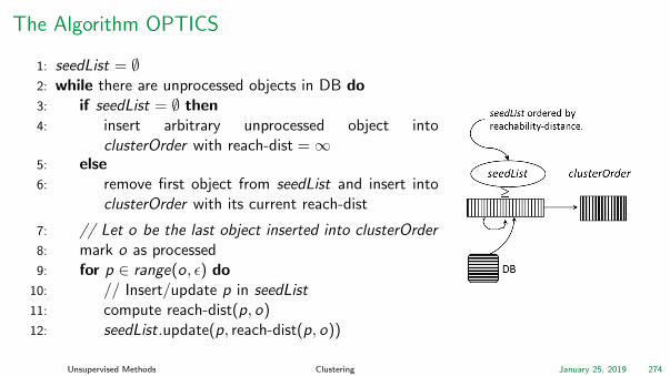
The Algorithm OPTICS
1: seedList = ∅2: while there are unprocessed objects in DB do3: if seedList = ∅ then4: insert arbitrary unprocessed object into
clusterOrder with reach-dist =∞5: else6: remove first object from seedList and insert into
clusterOrder with its current reach-dist
7: // Let o be the last object inserted into clusterOrder8: mark o as processed9: for p ∈ range(o, ε) do
10: // Insert/update p in seedList11: compute reach-dist(p, o)12: seedList.update(p, reach-dist(p, o))
Unsupervised Methods Clustering January 25, 2019 274

OPTICS: Exampleε = 44,MinPts = 3
Unsupervised Methods Clustering January 25, 2019 275

OPTICS: The Reachability Plot
Unsupervised Methods Clustering January 25, 2019 276

OPTICS: The Reachability Plot
I Plot the points together with their reachability-distances. Use the order in whichthey where returned by the algorithmI Represents the density-based clustering structureI Easy to analyzeI Independent of the dimensionality of the data
Unsupervised Methods Clustering January 25, 2019 277

OPTICS: Parameter Sensitivity
I Relatively insensitive to parameter settings
I Good result if parameters are just ”large enough”
Unsupervised Methods Clustering January 25, 2019 278

Hierarchical Clustering: Discussion
Advantages
I Does not require the number of clusters to be known in advanceI No (standard methods) or very robust parameters (OPTICS)I Computes a complete hierarchy of clustersI Good result visualizations integrated into the methodsI A ”flat” partition can be derived afterwards (e.g. via a cut through the
dendrogram or the reachability plot)
Disadvantages
I May not scale wellI Runtime for the standard methods: O(n2 log n2)I Runtime for OPTICS: without index support O(n2)
I User has to choose the final clustering
Unsupervised Methods Clustering January 25, 2019 279

Agenda
1. Introduction
2. Basics
3. Unsupervised Methods3.1 Frequent Pattern Mining3.2 Clustering
3.2.1 Partitioning Methods3.2.2 Probabilistic Model-Based Methods3.2.3 Density-Based Methods3.2.4 Mean-Shift3.2.5 Spectral Clustering3.2.6 Hierarchical Methods3.2.7 Evaluation3.2.8 Ensemble Clustering
3.3 Outlier Detection
4. Supervised Methods
5. Advanced Topics

Evaluation of Clustering Results
Type Positive Negative
Expert’sOpinion
may reveal new insightinto the data
very expensive, resultsare not comparable
ExternalMeasures
objective evaluation needs ”ground truth”
InternalMeasures
no additional informa-tion needed
approaches optimizingthe evaluation criteriawill always be preferred
Expert’s Opinion
External Measure
Internal MeasureUnsupervised Methods Clustering January 25, 2019 280

External Measures
Notation
Given a data set D, a clustering C = C1, . . . ,Ck and ground truth G = G1, . . . ,Gl.
Problem
Since the cluster labels are ”artificial”, permuting them should not change the score.
Solution
Instead of comparing cluster and ground truth labels directly, consider all pairs ofobjects. Check whether they have the same label in G and if they have the same in C.
Unsupervised Methods Clustering January 25, 2019 281

Formalisation as Retrieval Problem
C1 C2 C3D
o
p
p′SC 3
∈ SC
With P = (o, p) ∈ D × D | o 6= p define:
I Same cluster label: SC = (o, p) ∈ P | ∃Ci ∈ C : o, p ⊆ CiI Different cluster label: SC = P \ SC
and analogously for G.
Unsupervised Methods Clustering January 25, 2019 282

Formalisation as Retrieval Problem
Define
I TP = |SC ∩ SG |(same cluster in both, ”true positives”)
I FP = |SC ∩ SG |(same cluster in C, different cluster in G, ”falsepositives”)
I TN = |SC ∩ SG |(different cluster in both, ”true negatives”)
I FN = |SC ∩ SG |(different cluster in C, same cluster in G, ”falsenegatives”)
SC SC
SG
SG
P
TP FN
FP TN
Unsupervised Methods Clustering January 25, 2019 283

External Measures
I Recall (0 ≤ rec ≤ 1, larger is better)
rec =TP
TP + FN=|SC ∩ SG ||SG |
I Precision (0 ≤ prec ≤ 1, larger is better)
prec =TP
TP + FP=|SC ∩ SG ||SC |
I F1-Measure (0 ≤ F1 ≤ 1, larger is better)
F1 =2 · rec · prec
rec + prec=
2|SC ∩ SG ||SC |+ |SG |
SC SC
SG
SG
P
TP FN
FP TN
Unsupervised Methods Clustering January 25, 2019 284

External Measures
I Rand Index (0 ≤ RI ≤ 1, larger is better):
RI (C | G) =TP + TN
TP + TN + FP + FN=|SC ∩ SG |+ |SC ∩ SG |
|P|
I Adjusted Rand Index (ARI): Compares RI (C,G) againstexpected (R,G) of random cluster assignment R.
I Jaccard Coefficient (0 ≤ JC ≤ 1, larger is better):
JC =TP
TP + FP + FN=
|SC ∩ SG ||P| − |SC ∩ SG |
SC SC
SG
SG
P
TP FN
FP TN
Unsupervised Methods Clustering January 25, 2019 285

External Measures
I Confusion Matrix / Contingency Table N ∈ Nk×l with Nij = |Ci ∩ Gj |G1 . . . Gl
C1 |C1 ∩ G1| . . . |C1 ∩ Gl |...
.... . .
Ck |Ck ∩ G1| |Ck ∩ Gl |
I Define Ni =l∑
j=1Nij (i.e. Ni = |Ci |)
I Define N =k∑
i=1Ni (i.e. N = |D|)
Unsupervised Methods Clustering January 25, 2019 286

External Measures
I (Shannon) Entropy:
H(C) = −∑Ci∈C
p(Ci ) log p(Ci ) = −∑Ci∈C
|Ci ||D|
log|Ci ||D|
= −k∑
i=1
Ni
Nlog
Ni
N
I Mutual Entropy:
H(C | G) = −∑Ci∈C
p(Ci )∑Gj∈G
p(Gj | Ci ) log p(Gj | Ci )
= −∑Ci∈C
|Ci ||D|
∑Gj∈G
|Ci ∩ Gj ||Ci |
log|Ci ∩ Gj ||Ci |
= −k∑
i=1
Ni
N
l∑j=1
Nij
Nilog
Nij
Ni
Unsupervised Methods Clustering January 25, 2019 287

External Measures
I Mutual Information:
I (C,G) = H(C)− H(C | G) = H(G)− H(G | C)
I Normalized Mutual Information (NMI) (0 ≤ NMI ≤ 1, larger is better):
NMI (C,G) =I (C,G)√
H(C)H(G)
I Adjusted Mutual Information (AMI): Compares MI (C,G) against expectedMI (R,G) of random cluster assignment R.
Unsupervised Methods Clustering January 25, 2019 288

Internal Measures: Cohesion
Notation
Let D be a set of size n = |D|, and let C = C1, . . . ,Ck be a partitioning of D.
Cohesion
Average distance between objects of the same cluster.
coh(Ci ) =
(|Ci |
2
)−1 ∑o,p∈Ci ,o 6=p
d(o, p)
Cohesion of clustering is equal to weighted mean of the clusters’cohesions.
coh(C) =k∑
i=1
|Ci |n
coh(Ci )
Unsupervised Methods Clustering January 25, 2019 289

Internal Measures: Separation
Separation
Separation between to clusters: Average distance between pairs
sep(Ci ,Cj ) =1
|Ci ||Cj |∑
o∈Ci ,p∈Cj
d(o, p)
Separation of one cluster: Minimum separation to another cluster:
sep(Ci ) = minj 6=i
sep(Ci ,Cj )
Separation of clustering is equal to weighted mean of the clusters’separations.
sep(C) =k∑
i=1
|Ci |n
sep(Ci )
Unsupervised Methods Clustering January 25, 2019 290

Evaluating the Distance Matrix
7.5 5.0 2.5 0.0 2.5 5.0
7.5
5.0
2.5
0.0
2.5
5.0
7.5
10.0
dataset(well separated)
0 20 40 60 80
0
20
40
60
80
0.0
2.5
5.0
7.5
10.0
12.5
15.0
17.5
Distance matrix(sorted by k-means cluster label)
after: Tan, Steinbach, Kumar: Introduction to Data Mining (Pearson, 2006)
Unsupervised Methods Clustering January 25, 2019 291

Evaluating the Distance Matrix
Distance matrices differ for different clustering approaches (here on random data)k-means EM DBSCAN Complete Link
0.0 0.2 0.4 0.6 0.8 1.0
0.0
0.2
0.4
0.6
0.8
1.0
0.0 0.2 0.4 0.6 0.8 1.0
0.0
0.2
0.4
0.6
0.8
1.0
0.0 0.2 0.4 0.6 0.8 1.0
0.0
0.2
0.4
0.6
0.8
1.0
0.0 0.2 0.4 0.6 0.8 1.0
0.0
0.2
0.4
0.6
0.8
1.0
0 20 40 60 80
0
20
40
60
80
0 20 40 60 80
0
20
40
60
80
0 20 40 60 80
0
20
40
60
80
0 20 40 60 80
0
20
40
60
80
after: Tan, Steinbach, Kumar: Introduction to Data Mining (Pearson, 2006)
Unsupervised Methods Clustering January 25, 2019 292
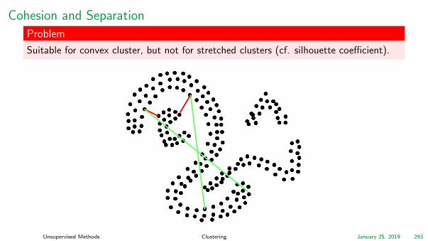
Cohesion and Separation
Problem
Suitable for convex cluster, but not for stretched clusters (cf. silhouette coefficient).
Unsupervised Methods Clustering January 25, 2019 293

Ambiguity of Clusterings
I Clustering according to: Color of shirt, direction of view, glasses, . . .
Unsupervised Methods Clustering January 25, 2019 294

Ambiguity of Clusterings
from: Tan, Steinbach, Kumar: Introduction to Data Mining (Pearson, 2006)
Unsupervised Methods Clustering January 25, 2019 295
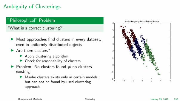
Ambiguity of Clusterings
”Philosophical” Problem
“What is a correct clustering?”
I Most approaches find clusters in every dataset,even in uniformly distributed objects
I Are there clusters?I Apply clustering algorithmI Check for reasonability of clusters
I Problem: No clusters found 6= no clustersexistingI Maybe clusters exists only in certain models,
but can not be found by used clusteringapproach
Unsupervised Methods Clustering January 25, 2019 296

Hopkins Statistics
Sample
dataset(n objects)
Random selection(m objects) m<<n
m uniformlydistributed objects
w3
w4
w5
w6
w1w2
u1
u2
u3u4
u5
u6
H =
m∑i=1
ui
m∑i=1
ui +m∑
i=1wi
I wi : distance of selected objects to the next neighbor in dataset
I ui : distances of uniformly distributed objects to next neighbor in dataset
I 0 ≤ H ≤ 1;I H ≈ 0: very regular data (e.g. grid);I H ≈ 0.5: uniformly distributed data;I H ≈ 1: strongly clusteredc
Unsupervised Methods Clustering January 25, 2019 297
Agenda
1. Introduction
2. Basics
3. Unsupervised Methods3.1 Frequent Pattern Mining3.2 Clustering
3.2.1 Partitioning Methods3.2.2 Probabilistic Model-Based Methods3.2.3 Density-Based Methods3.2.4 Mean-Shift3.2.5 Spectral Clustering3.2.6 Hierarchical Methods3.2.7 Evaluation3.2.8 Ensemble Clustering
3.3 Outlier Detection
4. Supervised Methods
5. Advanced Topics
Ensemble Clustering
Problem
I Many differing clustering models
I Different parameter choices, usually highly influences the result
What is a ”good” clustering?
Idea
Find a consensus solution (also ensemble clustering) that consolidates multipleclustering solutions.
Unsupervised Methods Clustering January 25, 2019 298
Ensemble Clustering: Benefits
I Knowledge Reuse: Possibility to integrate the knowledge of multiple known, goodclusterings
I Improved Quality: Often ensemble clustering leads to ”better” results than itsindividual base solutions.
I Improved Robustness: Combining several clustering approaches with differing datamodeling assumptions leads to an increased robustness across a wide range ofdatasets.
I Model Selection: Novel approach for determining the final number of clusters
I Distributed Clustering: if data is inherently distributed (either feature-wise orobject-wise) and each clusterer has only access to a subset of objects and/orfeatures, ensemble methods can be used to compute a unifying result
Unsupervised Methods Clustering January 25, 2019 299
Ensemble Clustering: Basic Notions
Given
A set of L clusterings C = C1, . . . , CL for dataset D = x1, . . . , xn ∈ Rd .
Goal
Find a consensus clustering C∗.
How to define a consensus clustering?
Two categories:
I Approaches based on pairwise similarity: Find a consensus clustering C∗ for whichthe similarity function Φ(C, C∗) =
∑C∈C
φ(C, C∗) (φ is basically an external measure)
I Probabilistic approaches: Assume that the L labels for the objects xi ∈ D follow acertain distribution.
Unsupervised Methods Clustering January 25, 2019 300

Similarity-Based Approaches
Goal
Find a consensus clustering C∗ for which the similarity functionΦ(C, C∗) =
∑C∈C
φ(C, C∗) is maximal.
Choices for φ
I Pair counting-based measures: Rand Index (RI), Adjusted RI, Probabilistic RI
I Information theoretic measures: Mutual Information (I), Normalized MutualInformation (NMI), Variation of Information (VI)
Problem
Minimising the objective for the above mentioned choices of φ in intractable.
Unsupervised Methods Clustering January 25, 2019 301

Similarity-Based Approaches
Solutions
I Methods based on the co-association matrix (related to RI)I Methods using cluster labels without co-association matrix (often related to NMI)
I Mostly graph partitioningI Cumulative voting
Unsupervised Methods Clustering January 25, 2019 302

Ensemble Clustering: Co-Association Matrix
Co-Association Matrix
The co-association matrix SC ∈ Rn×n represents the label similarity of object pairs:
SCij =
∑C∈C
I[xi ∈ C ∧ xj ∈ C]
where I is the indicator function with I[False] = 0, and I[True] = 1.
Example
D = 1, 2, 3, 4, 5 (i.e. n = 5),C = C1, C2,C1 = 1, 2, 3, 4, 5,C2 = 1, 2, 3, 4, 5.
S =
2 2 1 0 02 2 1 0 01 1 2 1 10 0 1 2 20 0 1 2 2
Unsupervised Methods Clustering January 25, 2019 303
Ensemble Clustering: Co-Association Matrix
Usage of Co-Association Matrix
I Use SC as similarity matrix to apply traditional clustering approach.
I By interpreting SC as weighted adjacency matrix, graph partitioning methods canbe applied.
Co-Association Matrix and Rand Index
In 16 a connection of consensus clustering based on the co-association matrix and theoptimization of the pairwise similarity based on the Rand Index has been proven:
Cbest = argmaxC∗
∑C∈C
RI (C, C∗)
16B. Mirkin: Mathematical Classification and Clustering. Kluwer, 1996.
Unsupervised Methods Clustering January 25, 2019 304

Information-Theoretic Approaches
Setting
Find a consensus clustering C∗ for which the similarity function Φ(C, C∗) =∑C∈C
φ(C, C∗)
is maximal, with φ chosen as (Normalised) Mutual Information.
Problem
Usually a hard optimization problem!
Solution 1
Use meaningful optimization approaches (e.g. gradient descent) or heuristics toapproximate the best clustering solution (e.g. 17)
17A. Strehl, J. Ghosh: Cluster ensembles - a knowledge reuse framework for combining multiple partitions. Journal of Machine Learning
Research, 3, 2002, pp. 583-617.
Unsupervised Methods Clustering January 25, 2019 305
Information-Theoretic Approaches
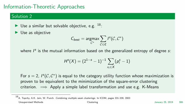
Solution 2
I Use a similar but solvable objective, e.g. 18:
I Use as objective
Cbest = argmaxC∗
∑C∈C
I s(C, C∗)
where I s is the mutual information based on the generalized entropy of degree s:
Hs(X ) = (21−s − 1)−1∑xi∈X
(psi − 1)
For s = 2, I s(C, C∗) is equal to the category utility function whose maximization isproven to be equivalent to the minimization of the square-error clusteringcriterion. =⇒ Apply a simple label transformation and use e.g. K-Means
18A. Topchy, A.K. Jain, W. Punch. Combining multiple weak clusterings. In ICDM, pages 331-339, 2003
Unsupervised Methods Clustering January 25, 2019 306

Probabilistic Approach
Assumptions
I All clusterings C ∈ C are partitionings of the dataset D.
I There are K∗ consensus clusters.
I With C(x) denoting the cluster label assigned to x in clustering C, the following datasetY given by
Y = yi ∈ NL0 | xi ∈ D,∀1 ≤ j ≤ L : (yi )j = Ci (xi )
(labels of base clusterings) follows a multivariate mixture distribution:
p(Y | Θ) =n∏
i=1
K∗∑k=1
αk pk (yi | θk )cond.ind.
=n∏
i=1
K∗∑k=1
αk
L∏j=1
pkl (yij | θkl )
with pkl (yij | θkl ) ∼ M(1, (pkl1, . . . , pkl|Cl |)), i.e. pkl (yij | θkl ) =|Cl |∏
k′=1
pI(ynl =k′)klk′
Unsupervised Methods Clustering January 25, 2019 307

Probabilistic Approach
Goal
Find the parameters Θ = (α1, θ1, . . . , αK∗, θK∗) such that the likelihood p(Y | Θ) ismaximized.
Solution 19
Optimize the parameters via the EM approach
19Topchy, Jain, Punch: A mixture model for clustering ensembles. In ICDM, pp. 379-390, 2004.
Unsupervised Methods Clustering January 25, 2019 308

Agenda
1. Introduction
2. Basics
3. Unsupervised Methods3.1 Frequent Pattern Mining3.2 Clustering3.3 Outlier Detection
3.3.1 Clustering-based Outliers3.3.2 Statistical Outliers3.3.3 Distance-based Outliers3.3.4 Density-based Outliers3.3.5 Angle-based Outliers3.3.6 Summary
4. Supervised Methods
5. Advanced Topics