data mining and knowledge discovery - ijskt.ijs.si/petrakralj/datamining0809/dm-2008.pdfdata mining...
TRANSCRIPT
Data Mining and Knowledge Discovery
Part of “New Media and e-Science” M.Sc. Programme
and “Statistics” M.Sc. Programme
2008 / 2009
Nada LavračJožef Stefan InstituteLjubljana, Slovenia
2
Course participantsI. IPS students• Aleksovski• Bole • Cimperman• Dali • Dervišević• Djuras• Dovgan• Kaluža• Mirčevska• Piltaver• Pollak• Rusu• Tomašev• Tomaško• Vukašinović• Zenkovič
II. Statistics students• Breznik• Golob• Korošec• Limbek• Ostrež• Suklan
3
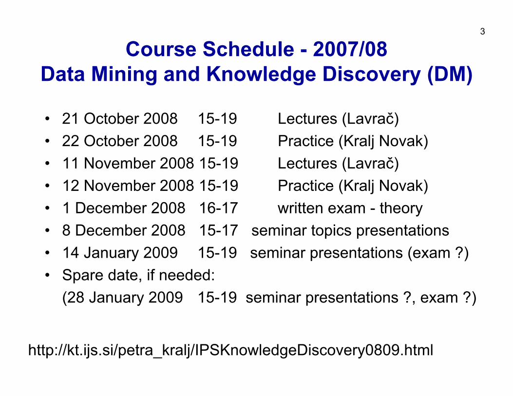
Course Schedule - 2007/08 Data Mining and Knowledge Discovery (DM)
• 21 October 2008 15-19 Lectures (Lavrač)• 22 October 2008 15-19 Practice (Kralj Novak)• 11 November 2008 15-19 Lectures (Lavrač)• 12 November 2008 15-19 Practice (Kralj Novak)• 1 December 2008 16-17 written exam - theory• 8 December 2008 15-17 seminar topics presentations• 14 January 2009 15-19 seminar presentations (exam ?)• Spare date, if needed:
(28 January 2009 15-19 seminar presentations ?, exam ?)
http://kt.ijs.si/petra_kralj/IPSKnowledgeDiscovery0809.html
4
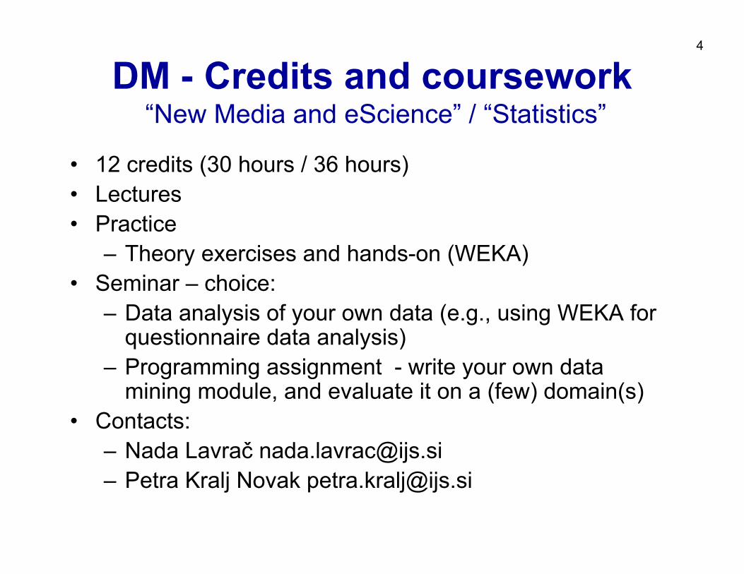
DM - Credits and coursework“New Media and eScience” / “Statistics”
• 12 credits (30 hours / 36 hours)• Lectures• Practice
– Theory exercises and hands-on (WEKA)• Seminar – choice:
– Data analysis of your own data (e.g., using WEKA for questionnaire data analysis)
– Programming assignment - write your own data mining module, and evaluate it on a (few) domain(s)
• Contacts: – Nada Lavrač [email protected]– Petra Kralj Novak [email protected]
5
DM - Credits and courseworkExam: Written exam (60 minutes) - Theory Seminar: topic selection + results presentation• Oral presentations of your seminar topic (DM task or
dataset presentation, max. 4 minutes)• Presentation of your seminar results (10 minutes +
discussion)• Deliver written report + electronic copy (in Information
Society paper format, see instructions on the web page), – Report on data analysis of own data needs to follow the
CRISP-DM methodology– Report on DM SW development needs to include SW
uploaded on a Web page – format to be announcedhttp://kt.ijs.si/petra_kralj/IPSKnowledgeDiscovery0809.html
6
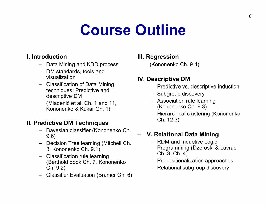
Course OutlineI. Introduction
– Data Mining and KDD process– DM standards, tools and
visualization– Classification of Data Mining
techniques: Predictive and descriptive DM(Mladenić et al. Ch. 1 and 11, Kononenko & Kukar Ch. 1)
II. Predictive DM Techniques– Bayesian classifier (Kononenko Ch.
9.6)– Decision Tree learning (Mitchell Ch.
3, Kononenko Ch. 9.1)– Classification rule learning
(Berthold book Ch. 7, KononenkoCh. 9.2)
– Classifier Evaluation (Bramer Ch. 6)
III. Regression (Kononenko Ch. 9.4)
IV. Descriptive DM– Predictive vs. descriptive induction– Subgroup discovery– Association rule learning
(Kononenko Ch. 9.3)– Hierarchical clustering (Kononenko
Ch. 12.3)
– V. Relational Data Mining– RDM and Inductive Logic
Programming (Dzeroski & LavracCh. 3, Ch. 4)
– Propositionalization approaches – Relational subgroup discovery
7
Part I. Introduction
Data Mining and the KDD process• DM standards, tools and visualization• Classification of Data Mining techniques:
Predictive and descriptive DM
8
What is DM
• Extraction of useful information from data: discovering relationships that have not previously been known
• The viewpoint in this course: Data Mining is the application of Machine Learning techniques to solve real-life data analysis problems
9
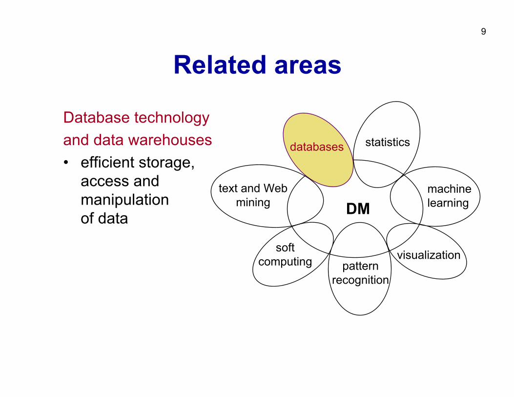
Related areas
Database technologyand data warehouses• efficient storage,
access and manipulationof data DM
statistics
machinelearning
visualization
text and Web mining
softcomputing pattern
recognition
databases
10
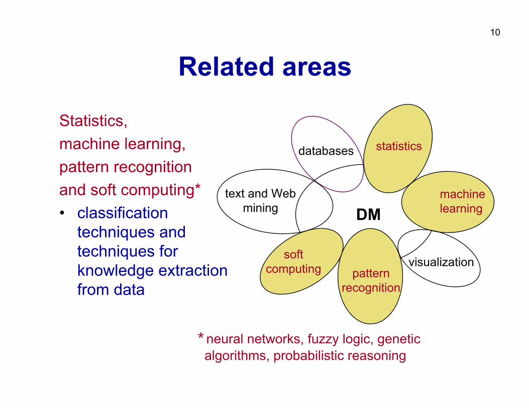
Statistics, machine learning,pattern recognitionand soft computing* • classification
techniques and techniques for knowledge extraction from data
* neural networks, fuzzy logic, geneticalgorithms, probabilistic reasoning
DM
statistics
machinelearning
visualization
text and Web mining
softcomputing pattern
recognition
databases
Related areas
11
DM
statistics
machinelearning
visualization
text and Web mining
softcomputing pattern
recognition
databases
Related areas
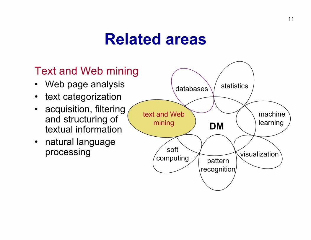
Text and Web mining• Web page analysis• text categorization• acquisition, filtering
and structuring of textual information
• natural language processing
text and Web mining
12
Related areas
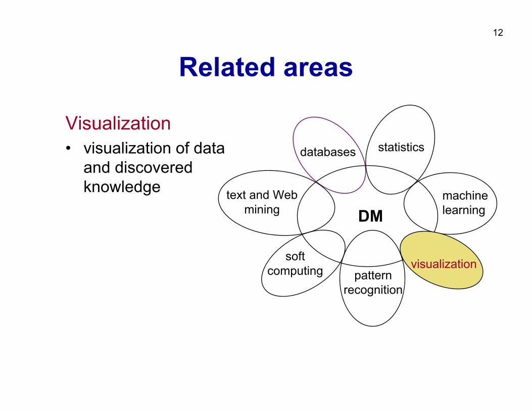
Visualization• visualization of data
and discovered knowledge
DM
statistics
machinelearning
visualization
text and Web mining
softcomputing pattern
recognition
databases
13
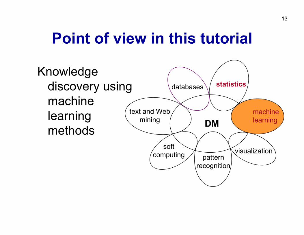
Point of view in this tutorial
Knowledge discovery using machine learning methods DM
statistics
machinelearning
visualization
text and Web mining
softcomputing pattern
recognition
databases
14
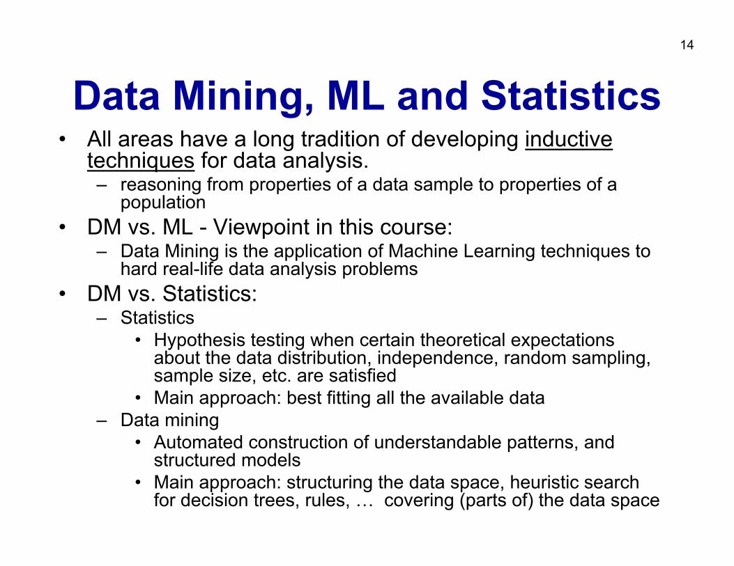
Data Mining, ML and Statistics• All areas have a long tradition of developing inductive
techniques for data analysis.– reasoning from properties of a data sample to properties of a
population• DM vs. ML - Viewpoint in this course:
– Data Mining is the application of Machine Learning techniques tohard real-life data analysis problems
• DM vs. Statistics:– Statistics
• Hypothesis testing when certain theoretical expectations about the data distribution, independence, random sampling, sample size, etc. are satisfied
• Main approach: best fitting all the available data– Data mining
• Automated construction of understandable patterns, and structured models
• Main approach: structuring the data space, heuristic search for decision trees, rules, … covering (parts of) the data space

15
Data Mining and KDD• KDD is defined as “the process of identifying
valid, novel, potentially useful and ultimately understandable models/patterns in data.” *
• Data Mining (DM) is the key step in the KDD process, performed by using data mining techniques for extracting models or interesting patterns from the data.
Usama M. Fayyad, Gregory Piatesky-Shapiro, Pedhraic Smyth: The KDD Process for Extracting Useful Knowledge form Volumes of Data. Comm ACM, Nov 96/Vol 39 No 11
16
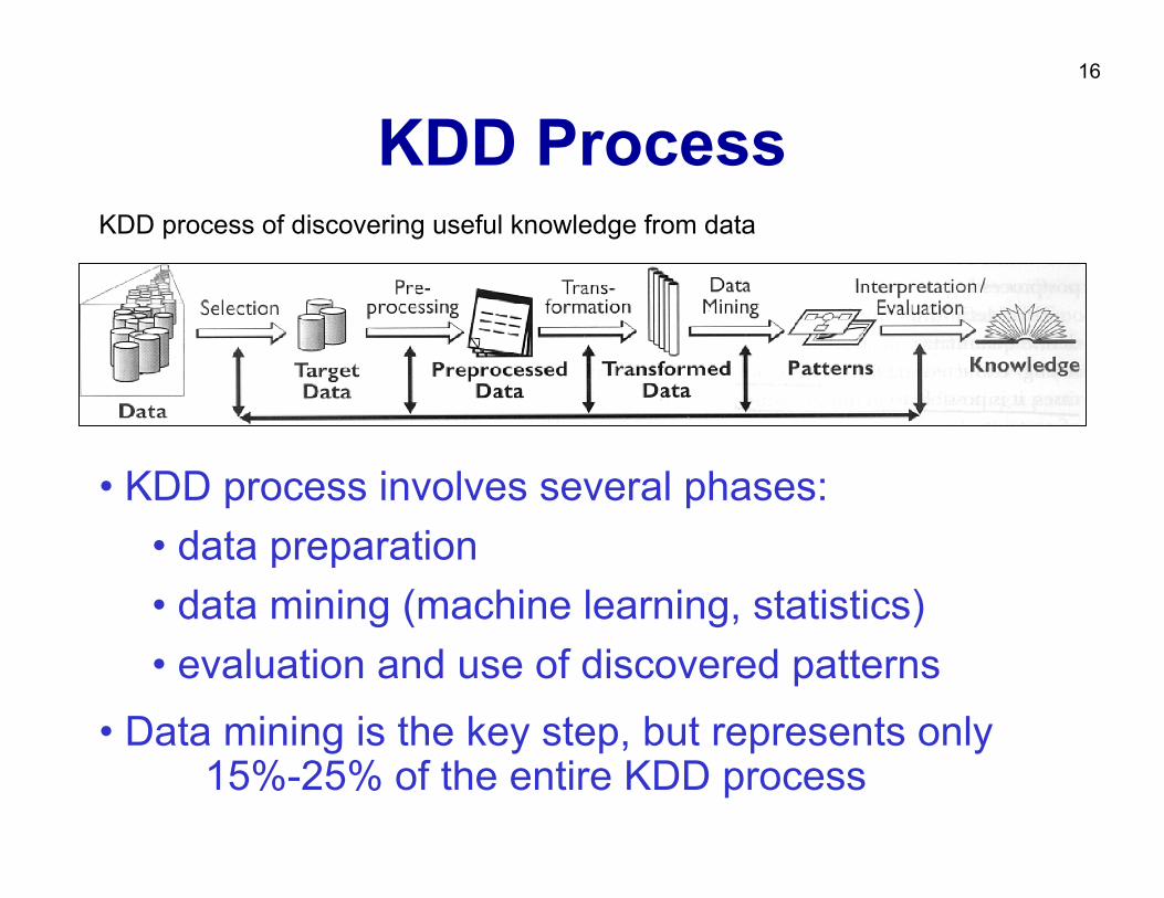
KDD ProcessKDD process of discovering useful knowledge from data
• KDD process involves several phases:• data preparation• data mining (machine learning, statistics)• evaluation and use of discovered patterns
• Data mining is the key step, but represents only 15%-25% of the entire KDD process
17
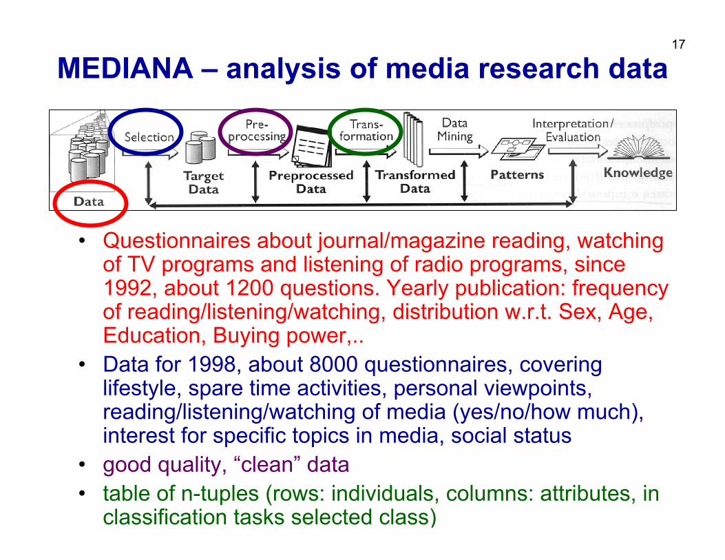
MEDIANA – analysis of media research data
• Questionnaires about journal/magazine reading, watching of TV programs and listening of radio programs, since 1992, about 1200 questions. Yearly publication: frequency of reading/listening/watching, distribution w.r.t. Sex, Age, Education, Buying power,..
• Data for 1998, about 8000 questionnaires, covering lifestyle, spare time activities, personal viewpoints, reading/listening/watching of media (yes/no/how much), interest for specific topics in media, social status
• good quality, “clean” data• table of n-tuples (rows: individuals, columns: attributes, in
classification tasks selected class)
18
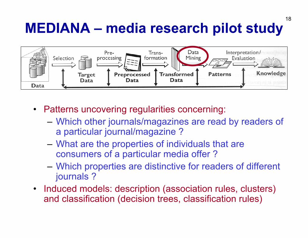
MEDIANA – media research pilot study
• Patterns uncovering regularities concerning:– Which other journals/magazines are read by readers of
a particular journal/magazine ?– What are the properties of individuals that are
consumers of a particular media offer ?– Which properties are distinctive for readers of different
journals ?• Induced models: description (association rules, clusters)
and classification (decision trees, classification rules)
19
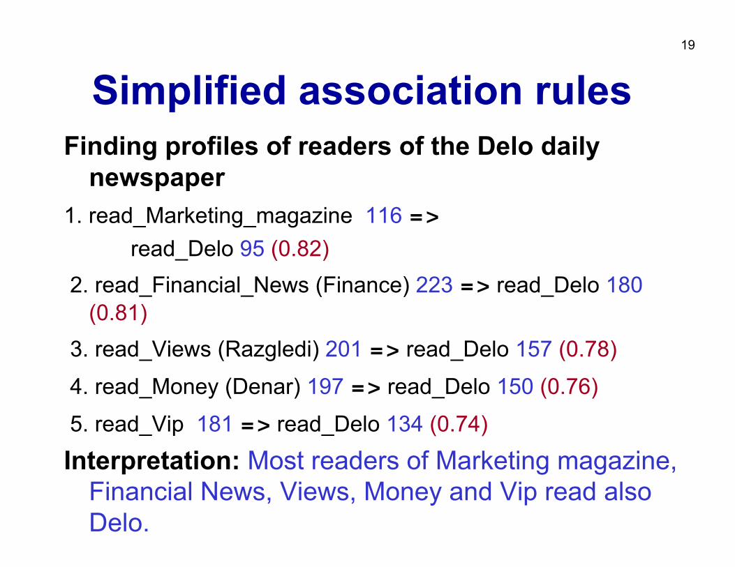
Simplified association rulesFinding profiles of readers of the Delo daily
newspaper1. read_Marketing_magazine 116 =>
read_Delo 95 (0.82)2. read_Financial_News (Finance) 223 => read_Delo 180
(0.81)3. read_Views (Razgledi) 201 => read_Delo 157 (0.78)
4. read_Money (Denar) 197 => read_Delo 150 (0.76)
5. read_Vip 181 => read_Delo 134 (0.74)
Interpretation: Most readers of Marketing magazine, Financial News, Views, Money and Vip read also Delo.
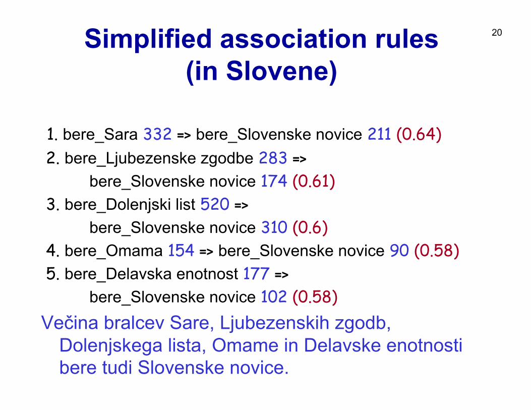
20Simplified association rules (in Slovene)
1. bere_Sara 332 => bere_Slovenske novice 211 (0.64)2. bere_Ljubezenske zgodbe 283 =>
bere_Slovenske novice 174 (0.61)3. bere_Dolenjski list 520 =>
bere_Slovenske novice 310 (0.6)4. bere_Omama 154 => bere_Slovenske novice 90 (0.58)5. bere_Delavska enotnost 177 =>
bere_Slovenske novice 102 (0.58)Večina bralcev Sare, Ljubezenskih zgodb,
Dolenjskega lista, Omame in Delavske enotnosti bere tudi Slovenske novice.
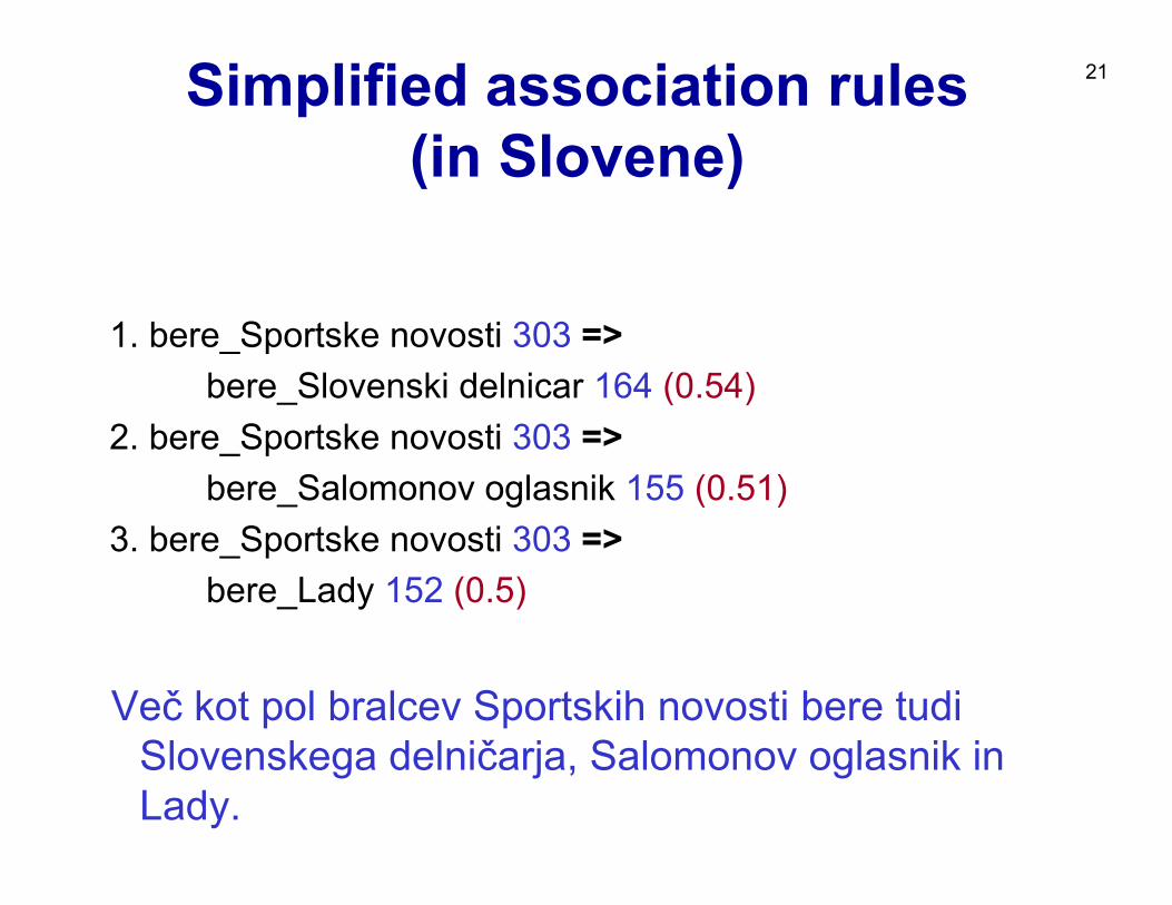
21Simplified association rules (in Slovene)
1. bere_Sportske novosti 303 =>bere_Slovenski delnicar 164 (0.54)
2. bere_Sportske novosti 303 =>bere_Salomonov oglasnik 155 (0.51)
3. bere_Sportske novosti 303 =>bere_Lady 152 (0.5)
Več kot pol bralcev Sportskih novosti bere tudi Slovenskega delničarja, Salomonov oglasnik in Lady.
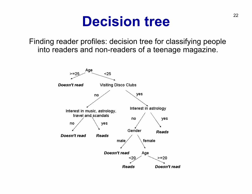
22Decision treeFinding reader profiles: decision tree for classifying people
into readers and non-readers of a teenage magazine.
23
Part I. Introduction
Data Mining and the KDD process• DM standards, tools and visualization• Classification of Data Mining techniques:
Predictive and descriptive DM
24
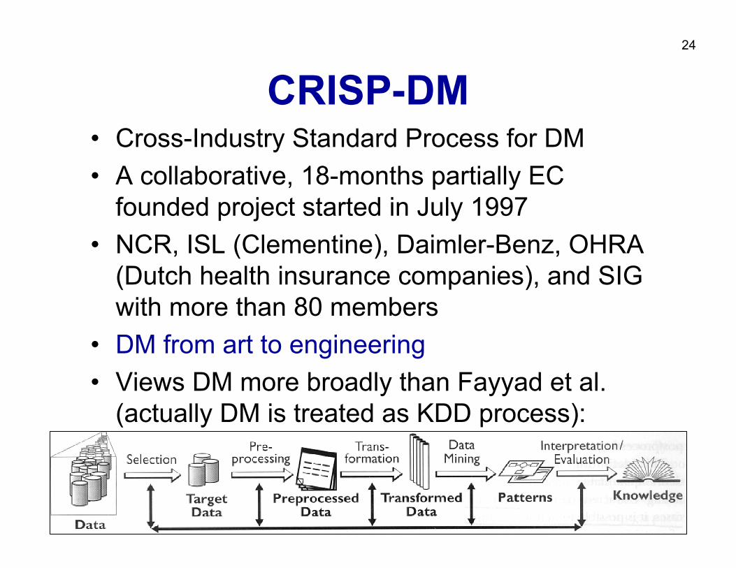
CRISP-DM• Cross-Industry Standard Process for DM• A collaborative, 18-months partially EC
founded project started in July 1997• NCR, ISL (Clementine), Daimler-Benz, OHRA
(Dutch health insurance companies), and SIG with more than 80 members
• DM from art to engineering• Views DM more broadly than Fayyad et al.
(actually DM is treated as KDD process):
25
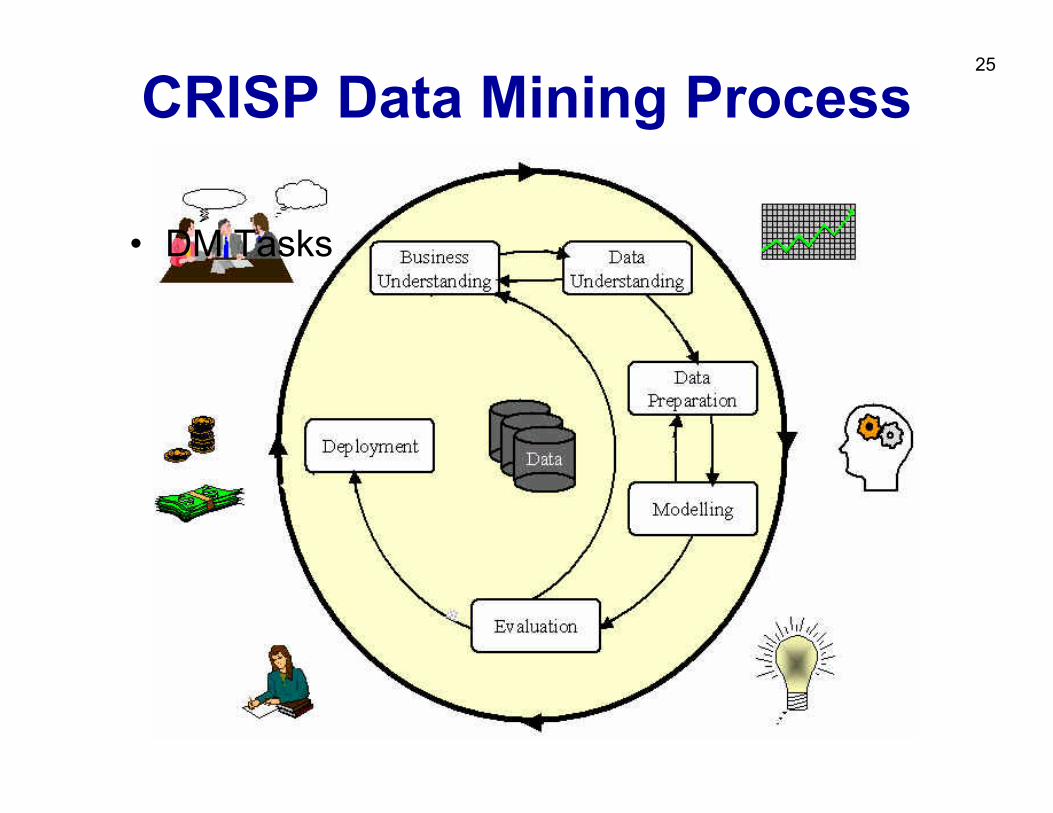
CRISP Data Mining Process
• DM Tasks
26
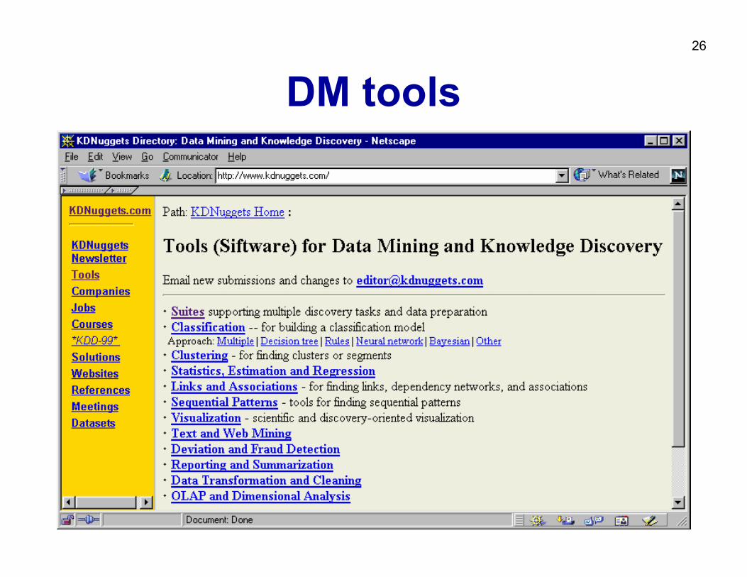
DM tools
27
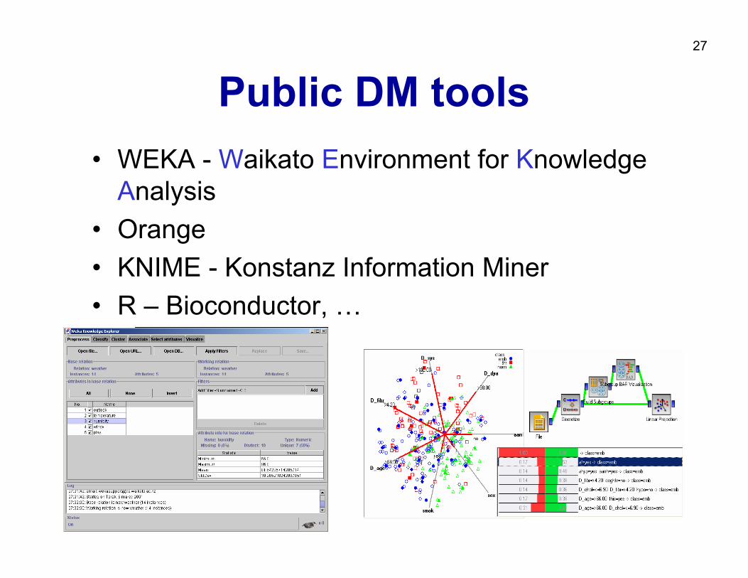
Public DM tools• WEKA - Waikato Environment for Knowledge
Analysis• Orange• KNIME - Konstanz Information Miner • R – Bioconductor, …
28
Visualization
• can be used on its own (usually for description and summarization tasks)
• can be used in combination with other DM techniques, for example– visualization of decision trees– cluster visualization– visualization of association rules– subgroup visualization
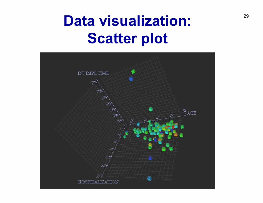
29Data visualization: Scatter plot
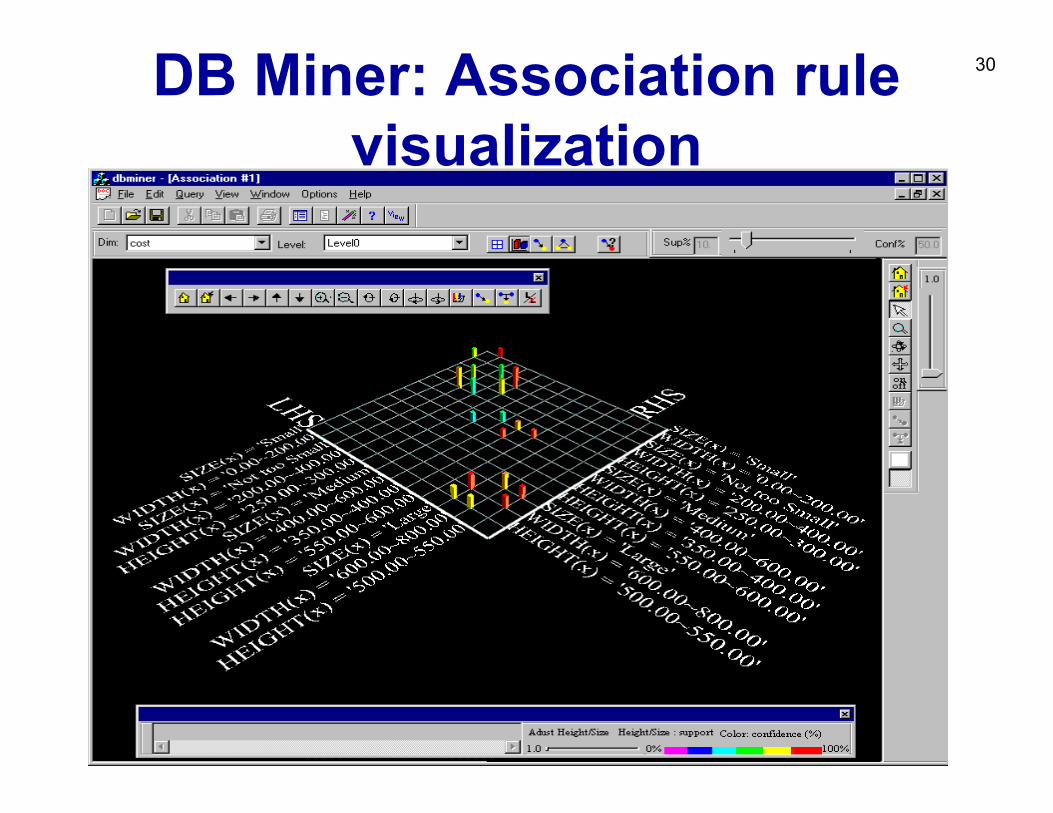
30DB Miner: Association rule visualization
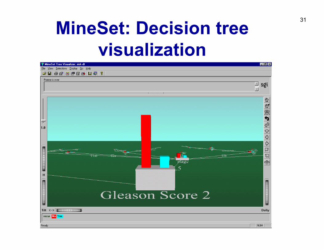
31MineSet: Decision tree visualization
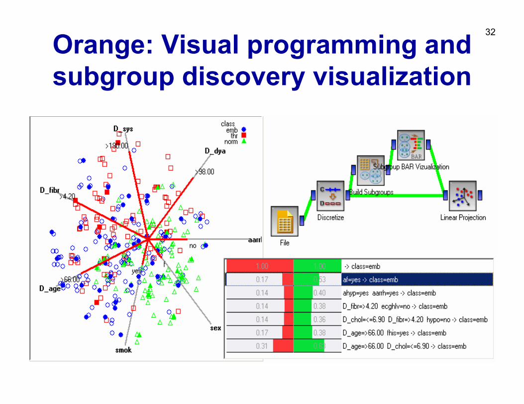
32Orange: Visual programming andsubgroup discovery visualization
33
Part I. Introduction
Data Mining and the KDD process• DM standards, tools and visualization• Classification of Data Mining techniques:
Predictive and descriptive DM
34
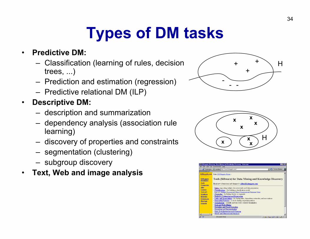
Types of DM tasks • Predictive DM:
– Classification (learning of rules, decision trees, ...)
– Prediction and estimation (regression)– Predictive relational DM (ILP)
• Descriptive DM:– description and summarization– dependency analysis (association rule
learning)– discovery of properties and constraints– segmentation (clustering)– subgroup discovery
• Text, Web and image analysis
++
+
---
H
xxx x
+xxx H
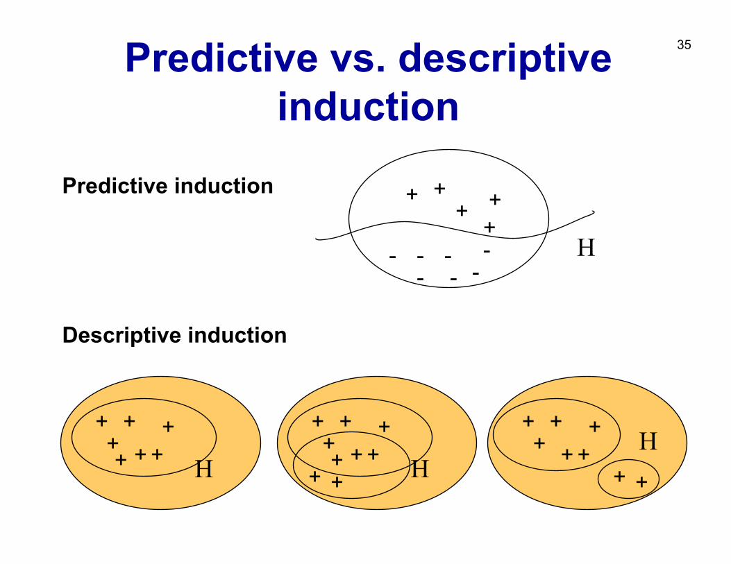
35Predictive vs. descriptive induction
Predictive induction
Descriptive induction
+
-
++ +
+- -
---
-Η
++ + +
+++Η+
++ + +
+++Η+
++
++ + +
+++ Η
++

36Predictive vs. descriptive induction
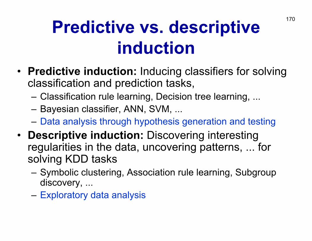
• Predictive induction: Inducing classifiers for solving classification and prediction tasks, – Classification rule learning, Decision tree learning, ...– Bayesian classifier, ANN, SVM, ...– Data analysis through hypothesis generation and testing
• Descriptive induction: Discovering interesting regularities in the data, uncovering patterns, ... for solving KDD tasks– Symbolic clustering, Association rule learning, Subgroup
discovery, ...– Exploratory data analysis
37
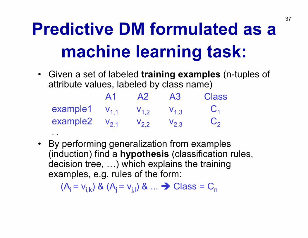
Predictive DM formulated as a machine learning task:
• Given a set of labeled training examples (n-tuples of attribute values, labeled by class name)
A1 A2 A3 Classexample1 v1,1 v1,2 v1,3 C1example2 v2,1 v2,2 v2,3 C2. .
• By performing generalization from examples (induction) find a hypothesis (classification rules, decision tree, …) which explains the training examples, e.g. rules of the form:
(Ai = vi,k) & (Aj = vj,l) & ... Class = Cn
38
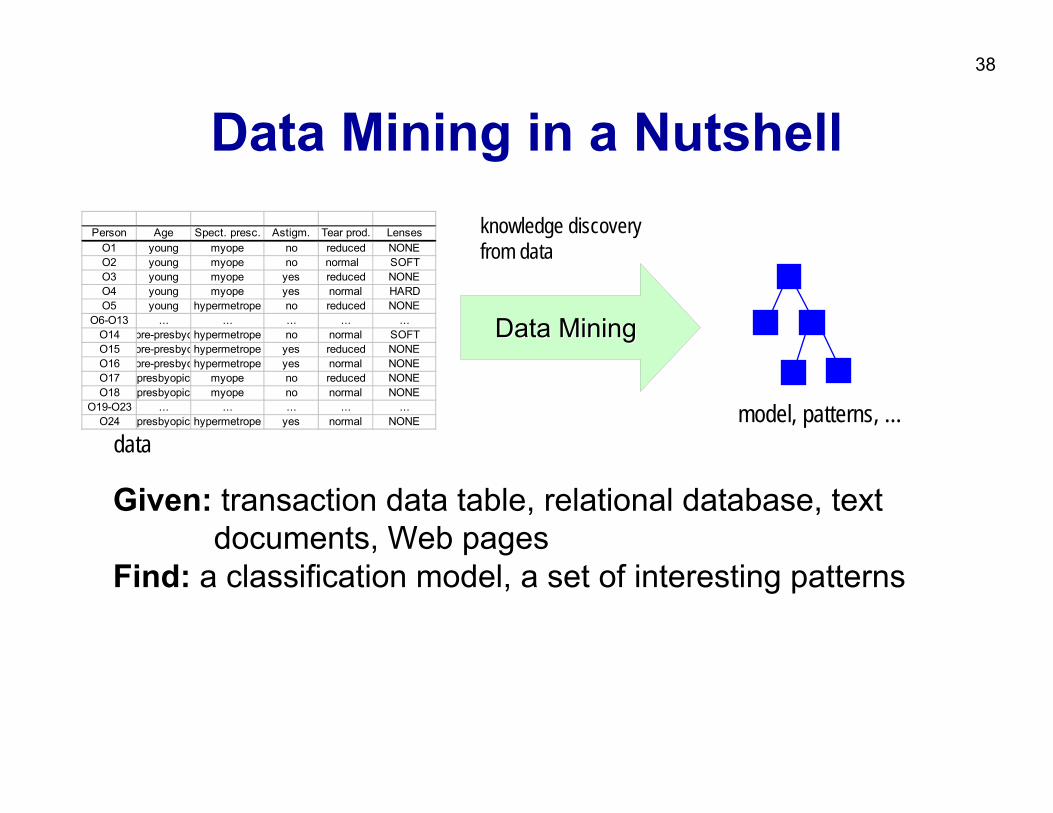
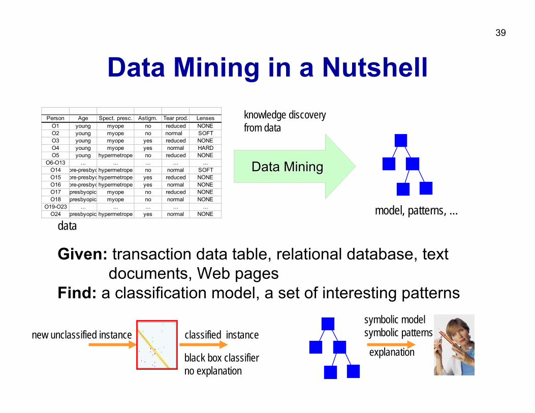
Data Mining in a Nutshell
data
Data MiningData Mining
knowledge discoveryfrom data
model, patterns, …
Given: transaction data table, relational database, textdocuments, Web pages
Find: a classification model, a set of interesting patterns
Person Age Spect. presc. Astigm. Tear prod. LensesO1 young myope no reduced NONEO2 young myope no normal SOFTO3 young myope yes reduced NONEO4 young myope yes normal HARDO5 young hypermetrope no reduced NONE
O6-O13 ... ... ... ... ...O14 pre-presbyohypermetrope no normal SOFTO15 pre-presbyohypermetrope yes reduced NONEO16 pre-presbyohypermetrope yes normal NONEO17 presbyopic myope no reduced NONEO18 presbyopic myope no normal NONE
O19-O23 ... ... ... ... ...O24 presbyopic hypermetrope yes normal NONE
39
Data Mining in a Nutshell
data
Data MiningData Mining
knowledge discoveryfrom data
model, patterns, …
Given: transaction data table, relational database, textdocuments, Web pages
Find: a classification model, a set of interesting patterns
Person Age Spect. presc. Astigm. Tear prod. LensesO1 young myope no reduced NONEO2 young myope no normal SOFTO3 young myope yes reduced NONEO4 young myope yes normal HARDO5 young hypermetrope no reduced NONE
O6-O13 ... ... ... ... ...O14 pre-presbyohypermetrope no normal SOFTO15 pre-presbyohypermetrope yes reduced NONEO16 pre-presbyohypermetrope yes normal NONEO17 presbyopic myope no reduced NONEO18 presbyopic myope no normal NONE
O19-O23 ... ... ... ... ...O24 presbyopic hypermetrope yes normal NONE
new unclassified instance classified instance
black box classifierno explanation
symbolic model symbolic patterns
explanation
40
Predictive DM - Classification
• data are objects, characterized with attributes -they belong to different classes (discrete labels)
• given objects described with attribute values, induce a model to predict different classes
• decision trees, if-then rules, discriminantanalysis, ...
41
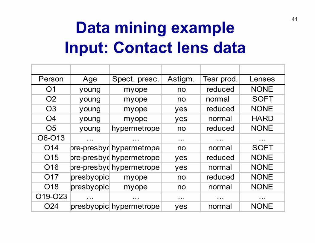
Data mining exampleInput: Contact lens data
Person Age Spect. presc. Astigm. Tear prod. LensesO1 young myope no reduced NONEO2 young myope no normal SOFTO3 young myope yes reduced NONEO4 young myope yes normal HARDO5 young hypermetrope no reduced NONE
O6-O13 ... ... ... ... ...O14 pre-presbyohypermetrope no normal SOFTO15 pre-presbyohypermetrope yes reduced NONEO16 pre-presbyohypermetrope yes normal NONEO17 presbyopic myope no reduced NONEO18 presbyopic myope no normal NONE
O19-O23 ... ... ... ... ...O24 presbyopic hypermetrope yes normal NONE
42
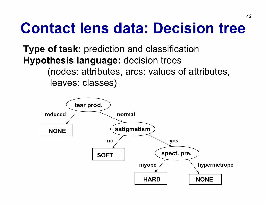
Contact lens data: Decision tree
tear prod.
astigmatism
spect. pre.
NONE
NONE
reduced
no yes
normal
hypermetrope
SOFTmyope
HARD
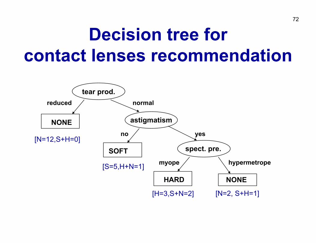
Type of task: prediction and classificationHypothesis language: decision trees
(nodes: attributes, arcs: values of attributes, leaves: classes)
43
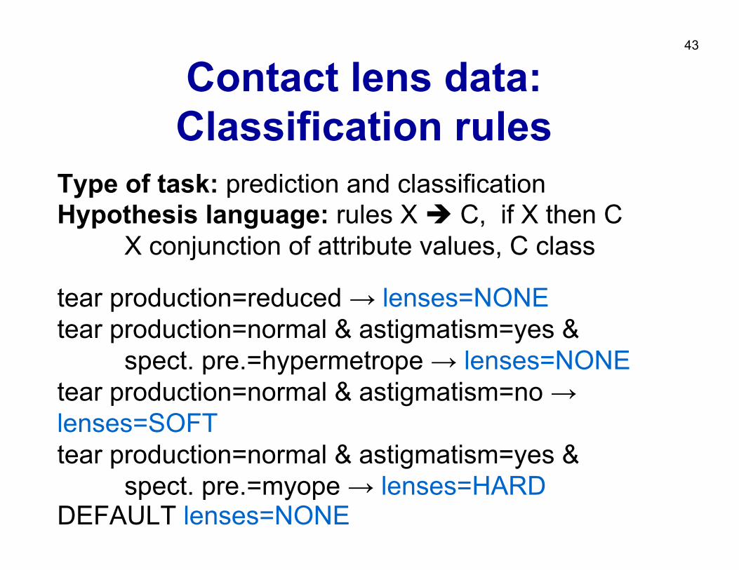
Contact lens data: Classification rules
Type of task: prediction and classificationHypothesis language: rules X C, if X then C
X conjunction of attribute values, C class
tear production=reduced → lenses=NONEtear production=normal & astigmatism=yes &
spect. pre.=hypermetrope → lenses=NONEtear production=normal & astigmatism=no →lenses=SOFTtear production=normal & astigmatism=yes &
spect. pre.=myope → lenses=HARDDEFAULT lenses=NONE
44
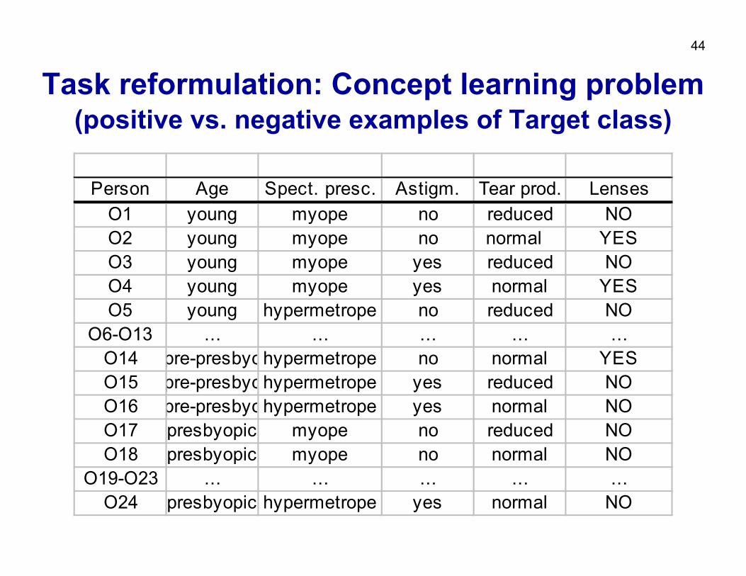
Task reformulation: Concept learning problem (positive vs. negative examples of Target class)
Person Age Spect. presc. Astigm. Tear prod. LensesO1 young myope no reduced NOO2 young myope no normal YESO3 young myope yes reduced NOO4 young myope yes normal YESO5 young hypermetrope no reduced NO
O6-O13 ... ... ... ... ...O14 pre-presbyohypermetrope no normal YESO15 pre-presbyohypermetrope yes reduced NOO16 pre-presbyohypermetrope yes normal NOO17 presbyopic myope no reduced NOO18 presbyopic myope no normal NO
O19-O23 ... ... ... ... ...O24 presbyopic hypermetrope yes normal NO
45
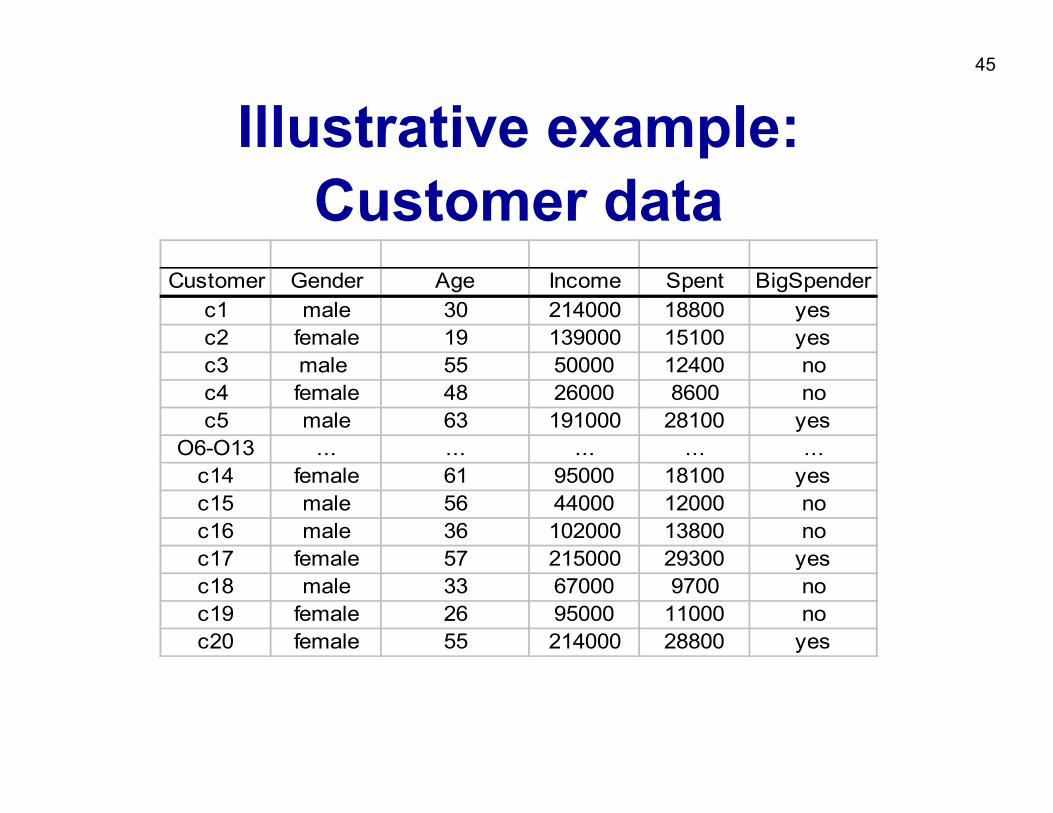
Illustrative example:Customer data
Customer Gender Age Income Spent BigSpenderc1 male 30 214000 18800 yesc2 female 19 139000 15100 yesc3 male 55 50000 12400 noc4 female 48 26000 8600 noc5 male 63 191000 28100 yes
O6-O13 ... ... ... ... ...c14 female 61 95000 18100 yesc15 male 56 44000 12000 noc16 male 36 102000 13800 noc17 female 57 215000 29300 yesc18 male 33 67000 9700 noc19 female 26 95000 11000 noc20 female 55 214000 28800 yes
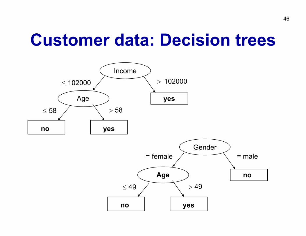
46
Customer data: Decision treesIncome
Age
no
yes
≤ 102000 > 102000
≤ 58 > 58
yes
Gender
Age
no
no
= female = male
≤ 49 > 49
yes
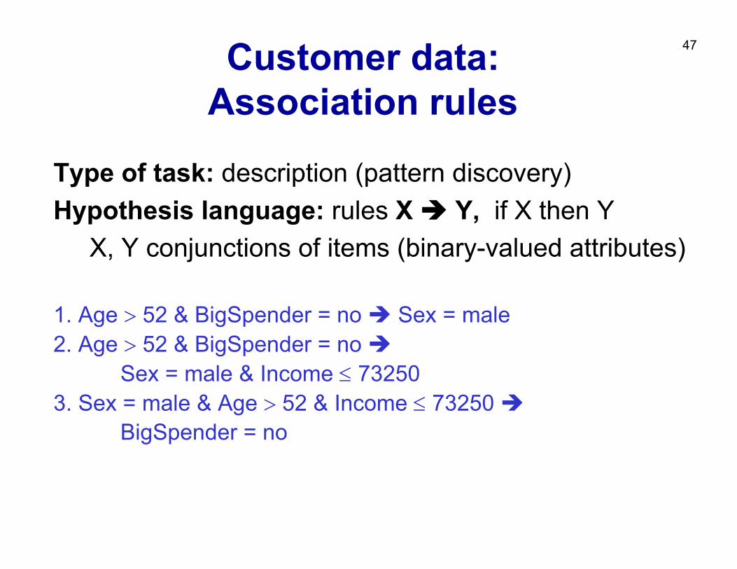
47Customer data: Association rules
Type of task: description (pattern discovery)Hypothesis language: rules X Y, if X then Y
X, Y conjunctions of items (binary-valued attributes)
1. Age > 52 & BigSpender = no Sex = male 2. Age > 52 & BigSpender = no
Sex = male & Income ≤ 732503. Sex = male & Age > 52 & Income ≤ 73250
BigSpender = no
48
Predictive DM - Estimation
• often referred to as regression• data are objects, characterized with attributes (discrete
or continuous), classes of objects are continuous (numeric)
• given objects described with attribute values, induce a model to predict the numeric class value
• regression trees, linear and logistic regression, ANN, kNN, ...
49
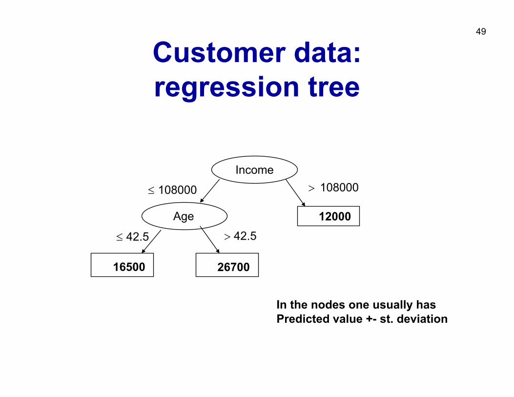
Customer data: regression tree
Income
Age
16500
12000
≤ 108000 > 108000
≤ 42.5 > 42.5
26700
In the nodes one usually has Predicted value +- st. deviation
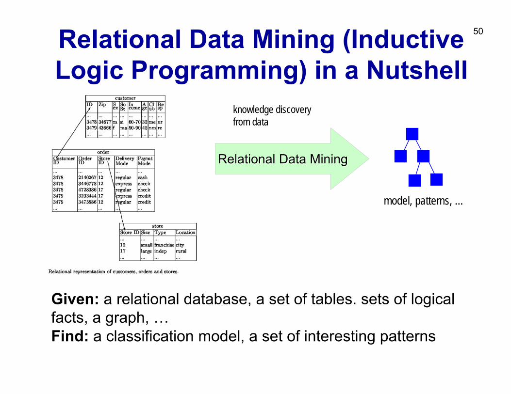
50Relational Data Mining (InductiveLogic Programming) in a Nutshell
RelationalRelational Data MiningData Mining
knowledge discoveryfrom data
model, patterns, …
Given: a relational database, a set of tables. sets of logicalfacts, a graph, …Find: a classification model, a set of interesting patterns
51
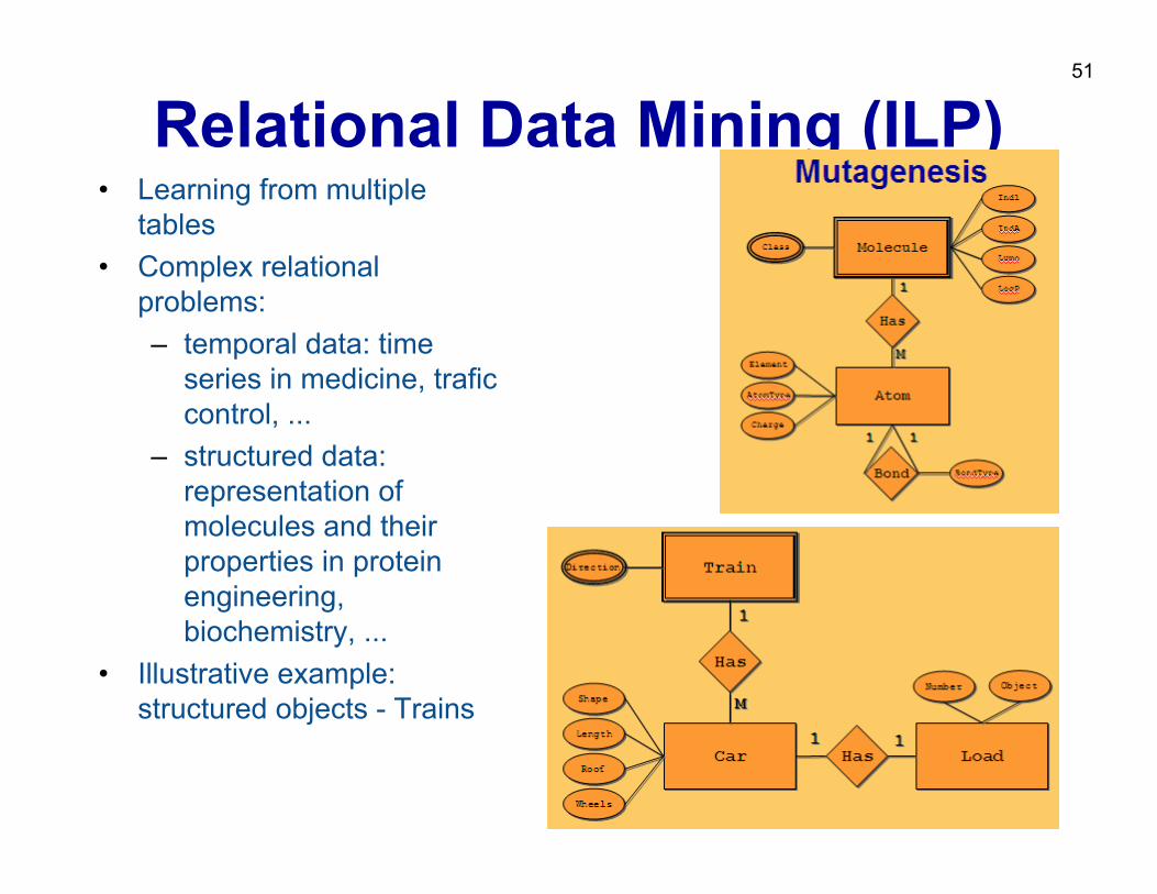
Relational Data Mining (ILP)• Learning from multiple
tables• Complex relational
problems:– temporal data: time
series in medicine, traficcontrol, ...
– structured data: representation of molecules and their properties in protein engineering, biochemistry, ...
• Illustrative example: structured objects - Trains
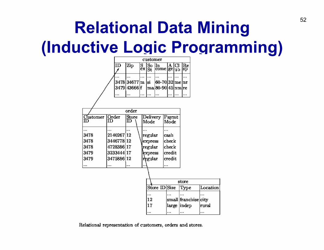
52Relational Data Mining (Inductive Logic Programming)
53
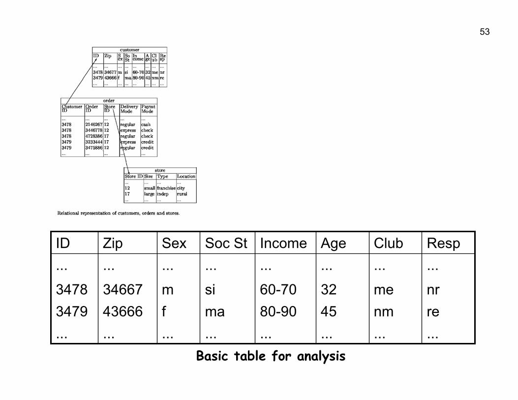
........................renm4580-90maf436663479nrme3260-70sim346673478
........................RespClubAgeIncomeSoc StSexZipID
Basic table for analysis
54
........................renm4580-90maf436663479nrme3260-70sim346673478
........................RespClubAgeIncomeSoc StSexZipID
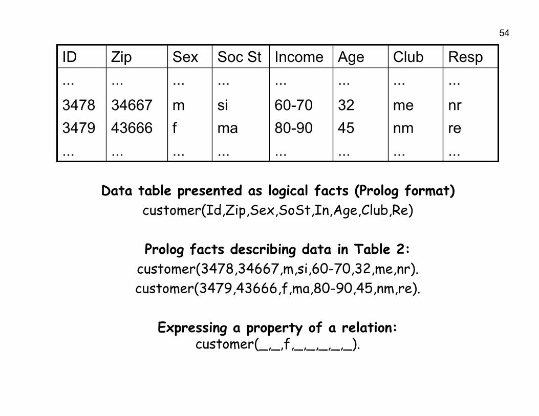
Data table presented as logical facts (Prolog format)customer(Id,Zip,Sex,SoSt,In,Age,Club,Re)
Prolog facts describing data in Table 2:customer(3478,34667,m,si,60-70,32,me,nr).customer(3479,43666,f,ma,80-90,45,nm,re).
Expressing a property of a relation:customer(_,_,f,_,_,_,_,_).
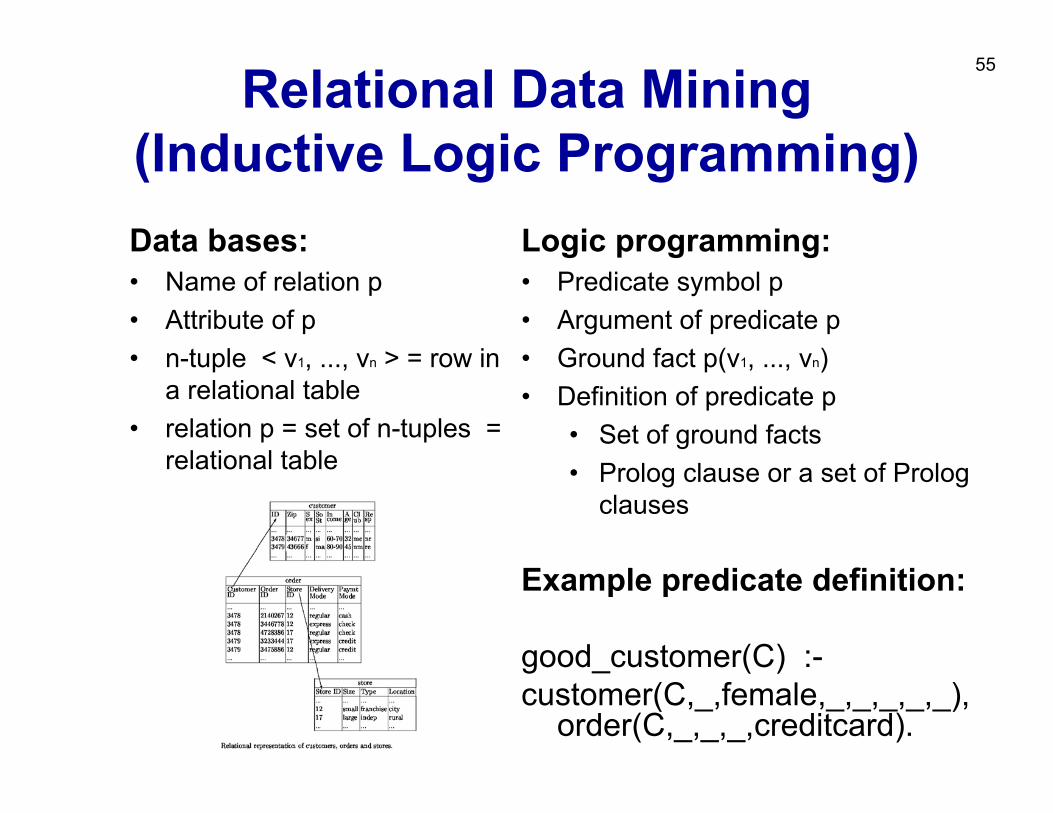
55Relational Data Mining (Inductive Logic Programming)
Logic programming:• Predicate symbol p• Argument of predicate p• Ground fact p(v1, ..., vn)• Definition of predicate p
• Set of ground facts• Prolog clause or a set of Prolog
clauses
Example predicate definition:
good_customer(C) :-customer(C,_,female,_,_,_,_,_),
order(C,_,_,_,creditcard).
Data bases:• Name of relation p• Attribute of p• n-tuple < v1, ..., vn > = row in
a relational table• relation p = set of n-tuples =
relational table
56
Part I: Summary• KDD is the overall process of discovering useful
knowledge in data– many steps including data preparation, cleaning,
transformation, pre-processing• Data Mining is the data analysis phase in KDD
– DM takes only 15%-25% of the effort of the overall KDD process
– employing techniques from machine learning and statistics• Predictive and descriptive induction have different
goals: classifier vs. pattern discovery• Many application areas• Many powerful tools available
57
Part II. Predictive DM techniques
• Naive Bayesian classifier• Decision tree learning• Classification rule learning• Classifier evaluation
58
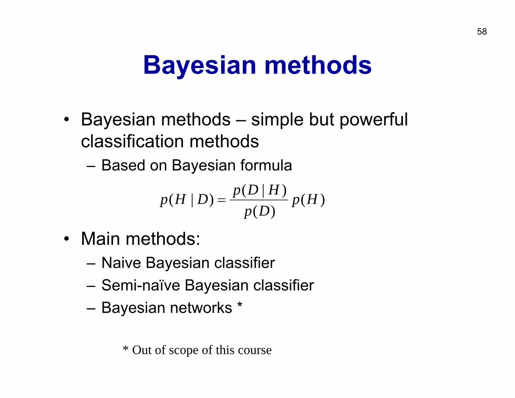
Bayesian methods
• Bayesian methods – simple but powerful classification methods– Based on Bayesian formula
• Main methods:– Naive Bayesian classifier– Semi-naïve Bayesian classifier– Bayesian networks *
* Out of scope of this course
)()(
)|()|( HpDp
HDpDHp =
59
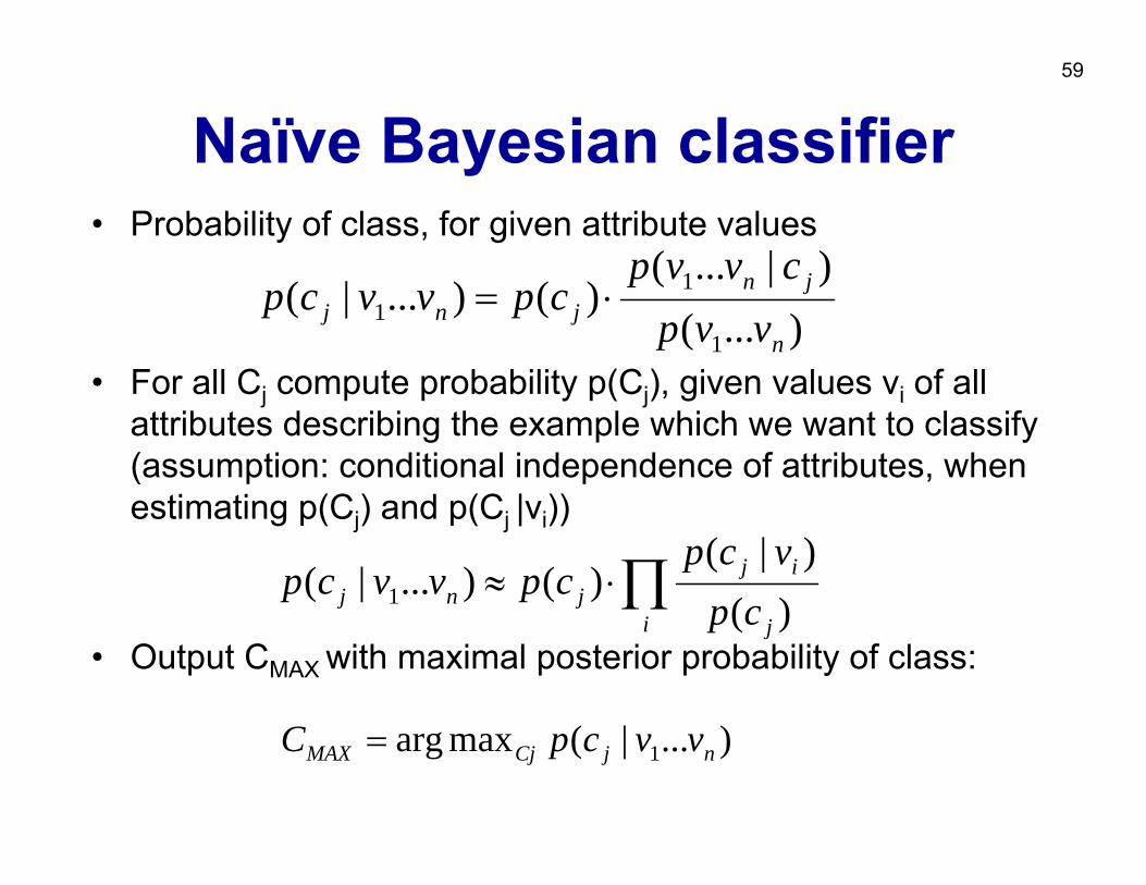
Naïve Bayesian classifier• Probability of class, for given attribute values
• For all Cj compute probability p(Cj), given values vi of all attributes describing the example which we want to classify (assumption: conditional independence of attributes, when estimating p(Cj) and p(Cj |vi))
• Output CMAX with maximal posterior probability of class:
)...()|...(
)()...|(1
11
n
jnjnj vvp
cvvpcpvvcp ⋅=
∏⋅≈i j
ijjnj cp
vcpcpvvcp
)()|(
)()...|( 1
)...|(maxarg 1 njCjMAX vvcpC =
60
Naïve Bayesian classifier
∏∏∏
∏∏
⋅≈⋅=
=⋅
=⋅
=
=⋅
=⋅
=
i j
ijj
i j
ij
n
ij
i j
iij
n
j
n
iiji
n
jjn
n
njnj
cpvcp
cpcp
vcpvvp
vpcp
cpvpvcp
vvpcp
vvp
cpcvpvvp
cpcvvpvvp
vvcpvvcp
)()|(
)()(
)|()...(
)()(
)()()|(
)...()(
)...(
)()|()...(
)()|...()...(
)...()...|(
1
11
1
1
1
11
61
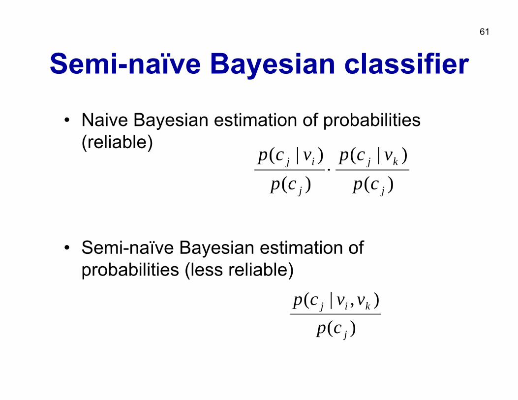
Semi-naïve Bayesian classifier
• Naive Bayesian estimation of probabilities (reliable)
• Semi-naïve Bayesian estimation of probabilities (less reliable)
)()|(
)()|(
j
kj
j
ij
cpvcp
cpvcp
⋅
)(),|(
j
kij
cpvvcp
62
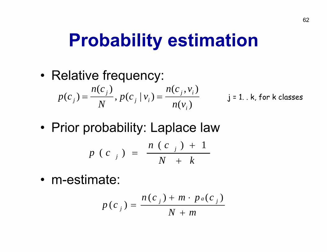
Probability estimation
• Relative frequency:
• Prior probability: Laplace law
• m-estimate:
)(),(
)|(,)(
)(i
ijij
jj vn
vcnvcp
Ncn
cp ==
mNcpmcn
cp jajj +
⋅+=
)()()(
kNcn
cp jj +
+=
1)()(
j = 1. . k, for k classes
63
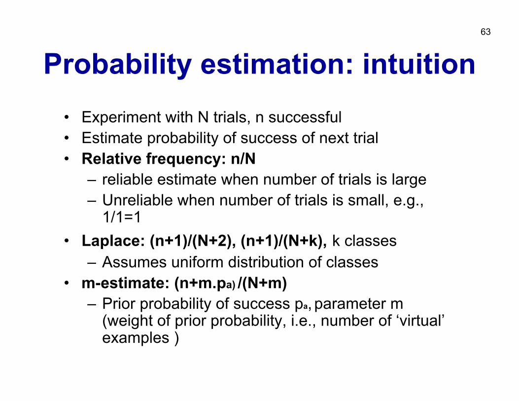
Probability estimation: intuition• Experiment with N trials, n successful• Estimate probability of success of next trial • Relative frequency: n/N
– reliable estimate when number of trials is large– Unreliable when number of trials is small, e.g.,
1/1=1• Laplace: (n+1)/(N+2), (n+1)/(N+k), k classes
– Assumes uniform distribution of classes• m-estimate: (n+m.pa) /(N+m)
– Prior probability of success pa, parameter m (weight of prior probability, i.e., number of ‘virtual’examples )
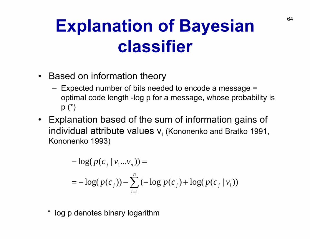
64Explanation of Bayesian classifier
• Based on information theory– Expected number of bits needed to encode a message =
optimal code length -log p for a message, whose probability is p (*)
• Explanation based of the sum of information gains of individual attribute values vi (Kononenko and Bratko 1991, Kononenko 1993)
* log p denotes binary logarithm
∑=
+−−−=
=−n
iijjj
nj
vcpcpcp
vvcp
1
1
))|(log()(log())(log(
))...|(log(

65
Example of explanation of semi-naïve Bayesian classifier
Hip surgery prognosisClass = no (“no complications”, most probable class, 2 class problem)
Attribute value For decision Against(bit) (bit)
Age = 70-80 0.07Sex = Female -0.19Mobility before injury = Fully mobile 0.04State of health before injury = Other 0.52Mechanism of injury = Simple fall -0.08Additional injuries = None 0Time between injury and operation > 10 days 0.42Fracture classification acc. To Garden = Garden III -0.3Fracture classification acc. To Pauwels = Pauwels III -0.14Transfusion = Yes 0.07Antibiotic profilaxies = Yes -0.32Hospital rehabilitation = Yes 0.05General complications = None 0Combination: 0.21 Time between injury and examination < 6 hours AND Hospitalization time between 4 and 5 weeksCombination: 0.63 Therapy = Artroplastic AND anticoagulant therapy = Yes
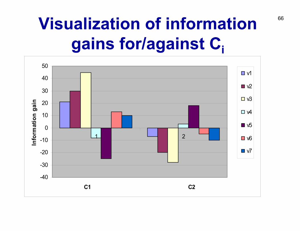
66Visualization of information gains for/against Ci
-40
-30
-20
-10
0
10
20
30
40
50
1 2
C1 C2
Info
rmat
ion
gain
v1
v2
v3
v4
v5
v6
v7
67
Naïve Bayesian classifier• Naïve Bayesian classifier can be used
– when we have sufficient number of training examples for reliable probability estimation
• It achieves good classification accuracy– can be used as ‘gold standard’ for comparison with
other classifiers• Resistant to noise (errors)
– Reliable probability estimation– Uses all available information
• Successful in many application domains– Web page and document classification – Medical diagnosis and prognosis, …
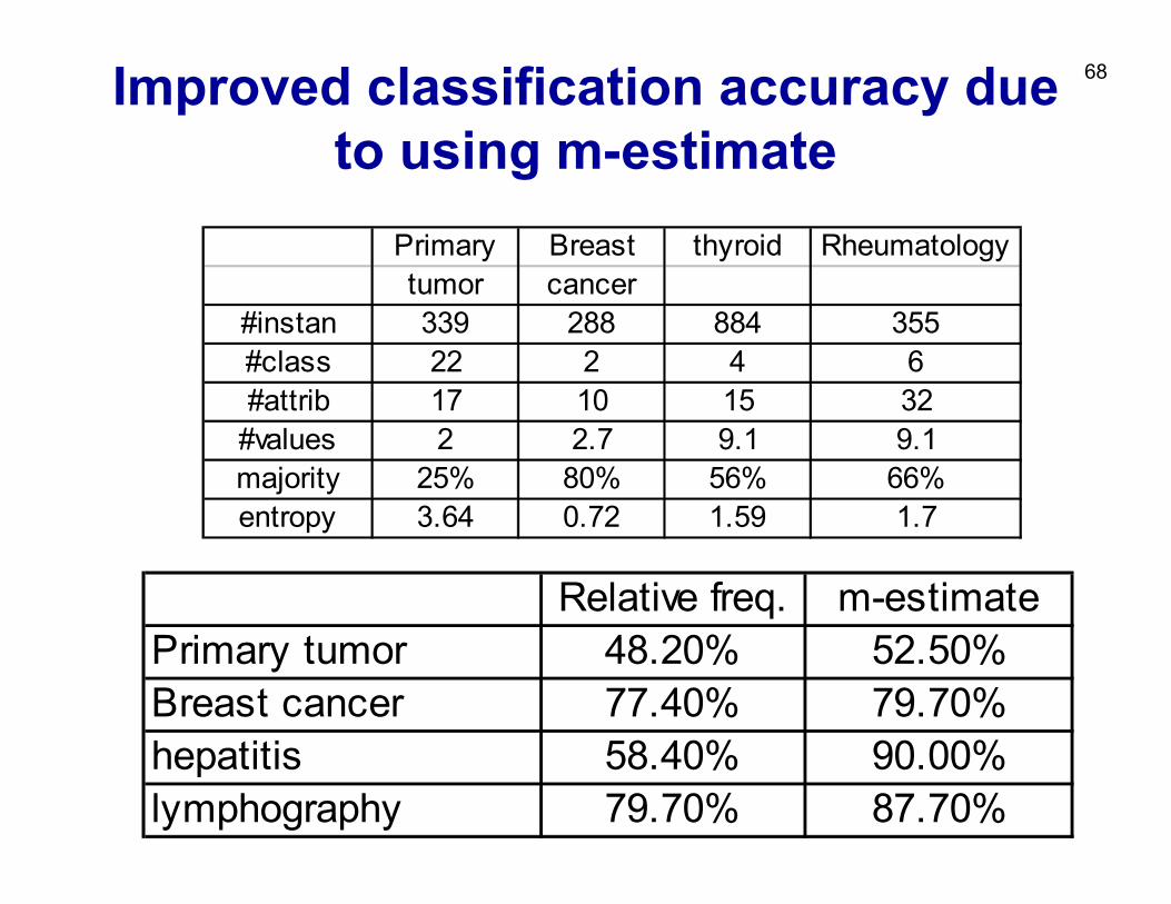
68Improved classification accuracy due to using m-estimate
Relative freq. m-estimatePrimary tumor 48.20% 52.50%Breast cancer 77.40% 79.70%hepatitis 58.40% 90.00%lymphography 79.70% 87.70%
Primary Breast thyroid Rheumatologytumor cancer
#instan 339 288 884 355#class 22 2 4 6#attrib 17 10 15 32
#values 2 2.7 9.1 9.1majority 25% 80% 56% 66%entropy 3.64 0.72 1.59 1.7
69
Part II. Predictive DM techniques
• Naïve Bayesian classifier• Decision tree learning• Classification rule learning• Classifier evaluation
70
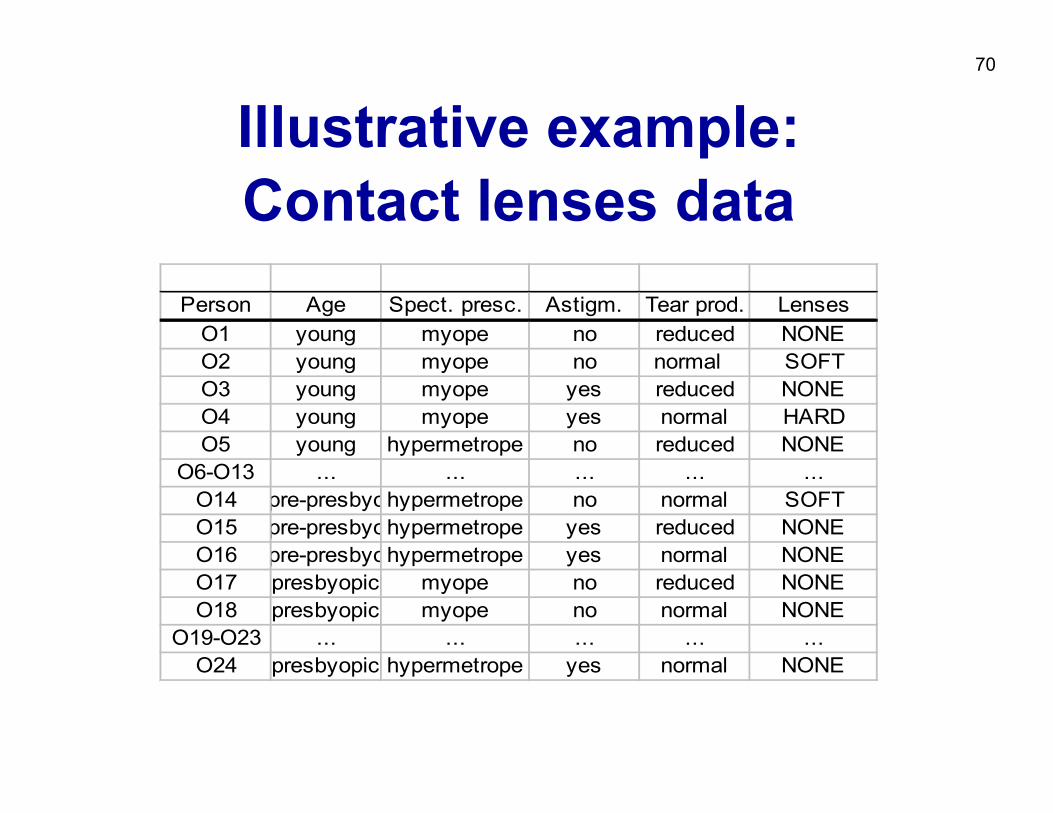
Illustrative example:Contact lenses data
Person Age Spect. presc. Astigm. Tear prod. LensesO1 young myope no reduced NONEO2 young myope no normal SOFTO3 young myope yes reduced NONEO4 young myope yes normal HARDO5 young hypermetrope no reduced NONE
O6-O13 ... ... ... ... ...O14 pre-presbyohypermetrope no normal SOFTO15 pre-presbyohypermetrope yes reduced NONEO16 pre-presbyohypermetrope yes normal NONEO17 presbyopic myope no reduced NONEO18 presbyopic myope no normal NONE
O19-O23 ... ... ... ... ...O24 presbyopic hypermetrope yes normal NONE
71
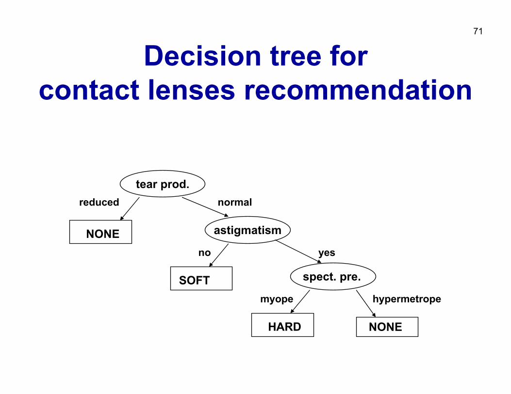
Decision tree forcontact lenses recommendation
tear prod.
astigmatism
spect. pre.
NONE
NONE
reduced
no yes
normal
hypermetrope
SOFTmyope
HARD
72
Decision tree forcontact lenses recommendation
tear prod.
astigmatism
spect. pre.
NONE
NONE
reduced
no yes
normal
hypermetrope
SOFTmyope
HARD
[N=12,S+H=0]
[N=2, S+H=1]
[S=5,H+N=1]
[H=3,S+N=2]
73
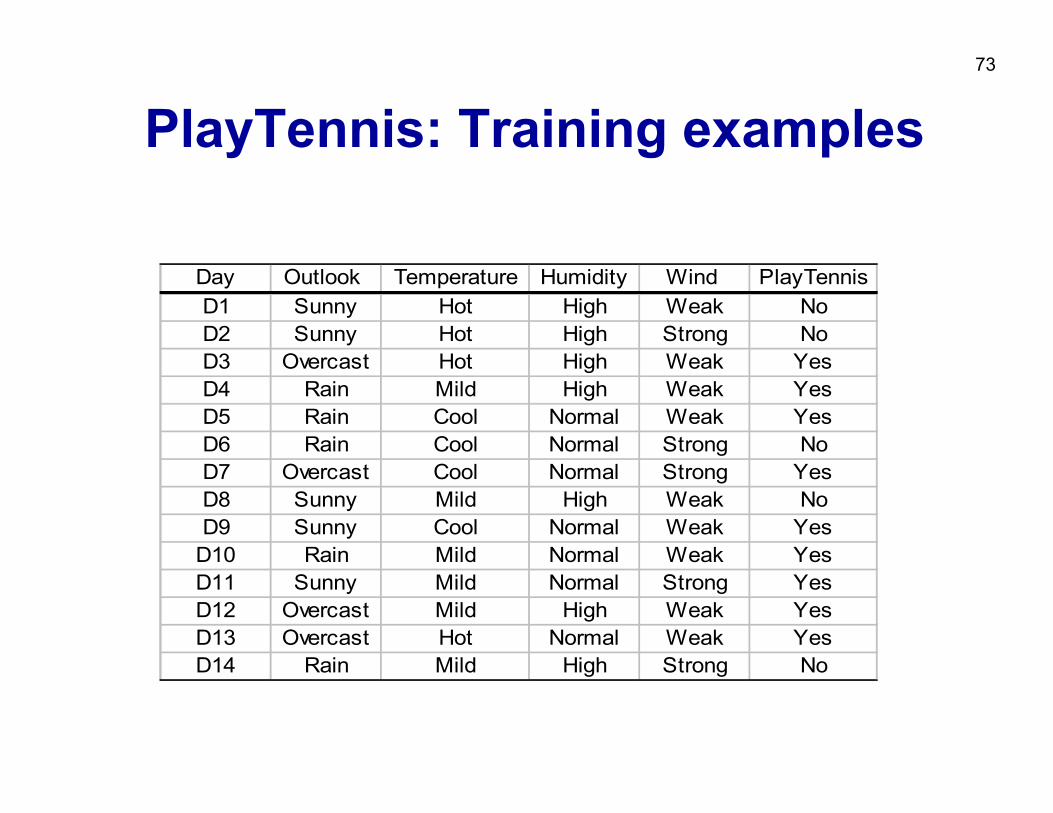
PlayTennis: Training examples
Day Outlook Temperature Humidity Wind PlayTennisD1 Sunny Hot High Weak NoD2 Sunny Hot High Strong NoD3 Overcast Hot High Weak YesD4 Rain Mild High Weak YesD5 Rain Cool Normal Weak YesD6 Rain Cool Normal Strong NoD7 Overcast Cool Normal Strong YesD8 Sunny Mild High Weak NoD9 Sunny Cool Normal Weak Yes
D10 Rain Mild Normal Weak YesD11 Sunny Mild Normal Strong YesD12 Overcast Mild High Weak YesD13 Overcast Hot Normal Weak YesD14 Rain Mild High Strong No
74
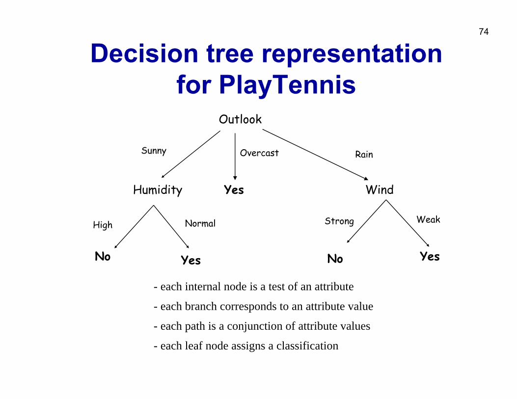
Decision tree representation for PlayTennis
Outlook
Humidity WindYes
OvercastSunny Rain
High Normal Strong Weak
No Yes No Yes
- each internal node is a test of an attribute
- each branch corresponds to an attribute value
- each path is a conjunction of attribute values
- each leaf node assigns a classification
75
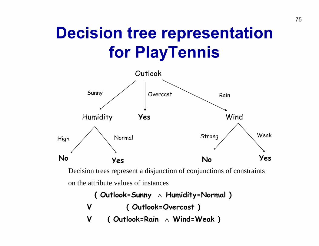
Decision tree representation for PlayTennis
Outlook
Humidity WindYes
OvercastSunny Rain
High Normal Strong Weak
No Yes No YesDecision trees represent a disjunction of conjunctions of constraints
on the attribute values of instances
( Outlook=Sunny ∧ Humidity=Normal ) V ( Outlook=Overcast )V ( Outlook=Rain ∧ Wind=Weak )
76
PlayTennis:Other representations
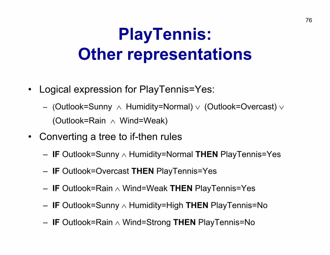
• Logical expression for PlayTennis=Yes:
– (Outlook=Sunny ∧ Humidity=Normal) ∨ (Outlook=Overcast) ∨
(Outlook=Rain ∧ Wind=Weak)
• Converting a tree to if-then rules
– IF Outlook=Sunny ∧ Humidity=Normal THEN PlayTennis=Yes
– IF Outlook=Overcast THEN PlayTennis=Yes
– IF Outlook=Rain ∧ Wind=Weak THEN PlayTennis=Yes
– IF Outlook=Sunny ∧ Humidity=High THEN PlayTennis=No
– IF Outlook=Rain ∧ Wind=Strong THEN PlayTennis=No
77
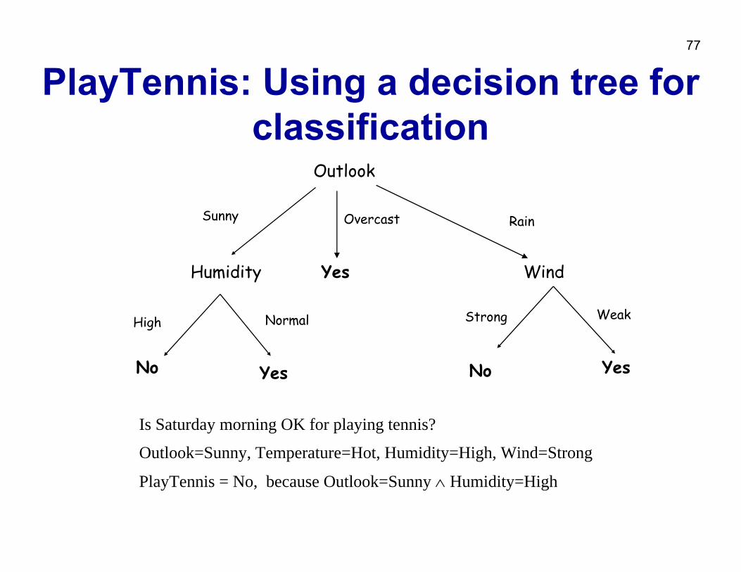
PlayTennis: Using a decision tree for classification
Is Saturday morning OK for playing tennis?
Outlook=Sunny, Temperature=Hot, Humidity=High, Wind=Strong
PlayTennis = No, because Outlook=Sunny ∧ Humidity=High
Outlook
Humidity WindYes
OvercastSunny Rain
High Normal Strong Weak
No Yes No Yes
78
Appropriate problems for decision tree learning
• Classification problems: classify an instance into one of a discrete set of possible categories (medical diagnosis, classifying loan applicants, …)
• Characteristics:– instances described by attribute-value pairs
(discrete or real-valued attributes)– target function has discrete output values
(boolean or multi-valued, if real-valued then regression trees)– disjunctive hypothesis may be required– training data may be noisy
(classification errors and/or errors in attribute values)– training data may contain missing attribute values
79
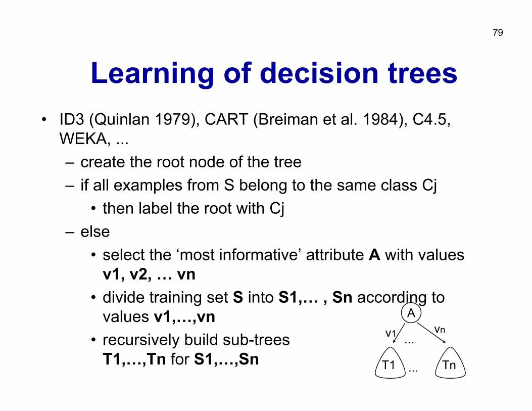
Learning of decision trees• ID3 (Quinlan 1979), CART (Breiman et al. 1984), C4.5,
WEKA, ...– create the root node of the tree– if all examples from S belong to the same class Cj
• then label the root with Cj– else
• select the ‘most informative’ attribute A with values v1, v2, … vn
• divide training set S into S1,… , Sn according to values v1,…,vn
• recursively build sub-treesT1,…,Tn for S1,…,Sn
A
...
...T1 Tn
vnv1
80
Search heuristics in ID3• Central choice in ID3: Which attribute to test at
each node in the tree ? The attribute that is most useful for classifying examples.
• Define a statistical property, called information gain, measuring how well a given attribute separates the training examples w.r.t their target classification.
• First define a measure commonly used in information theory, called entropy, to characterize the (im)purity of an arbitrary collection of examples.
81
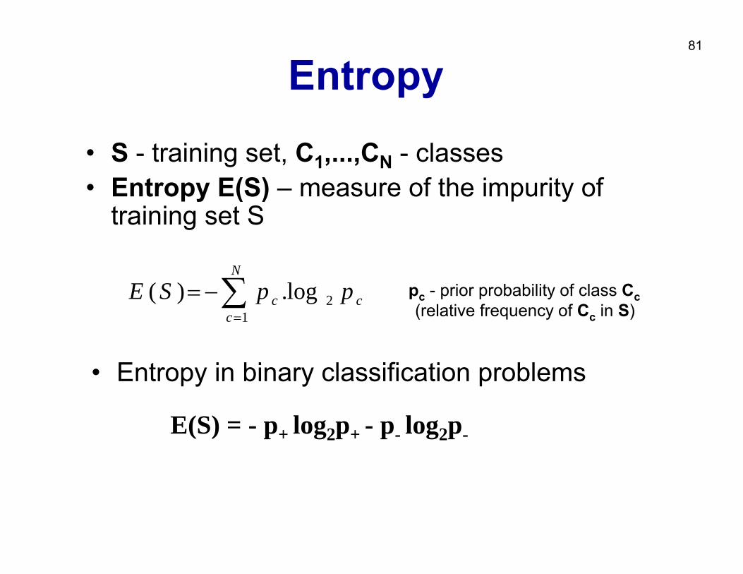
Entropy
• S - training set, C1,...,CN - classes• Entropy E(S) – measure of the impurity of
training set S
∑=
−=N
ccc ppSE
12log.)( pc - prior probability of class Cc
(relative frequency of Cc in S)
E(S) = - p+ log2p+ - p- log2p-
• Entropy in binary classification problems
82
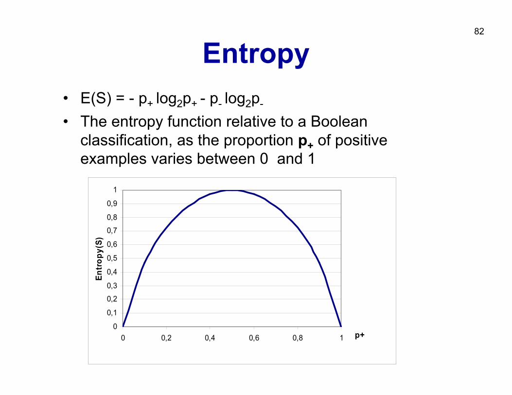
Entropy• E(S) = - p+ log2p+ - p- log2p-
• The entropy function relative to a Boolean classification, as the proportion p+ of positive examples varies between 0 and 1
0
0,1
0,2
0,3
0,4
0,5
0,6
0,7
0,8
0,9
1
0 0,2 0,4 0,6 0,8 1 p+
Entr
opy(
S)
83
Entropy – why ?• Entropy E(S) = expected amount of information (in
bits) needed to assign a class to a randomly drawn object in S (under the optimal, shortest-length code)
• Why ?• Information theory: optimal length code assigns
- log2p bits to a message having probability p• So, in binary classification problems, the expected
number of bits to encode + or – of a random member of S is:
p+ ( - log2p+ ) + p- ( - log2p- ) = - p+ log2p+ - p- log2p-
84
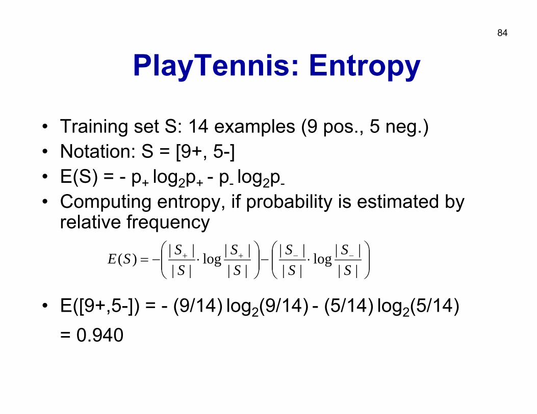
PlayTennis: Entropy
• Training set S: 14 examples (9 pos., 5 neg.)• Notation: S = [9+, 5-] • E(S) = - p+ log2p+ - p- log2p-• Computing entropy, if probability is estimated by
relative frequency
• E([9+,5-]) = - (9/14) log2(9/14) - (5/14) log2(5/14) = 0.940
⎟⎟⎠
⎞⎜⎜⎝
⎛⋅−⎟⎟
⎠
⎞⎜⎜⎝
⎛⋅−= −−++
||||log
||||
||||log
||||)(
SS
SS
SS
SSSE
85
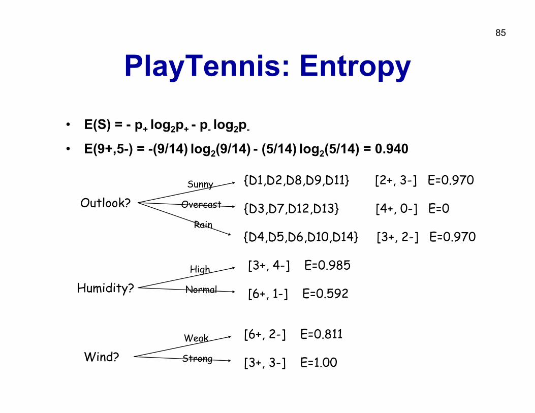
PlayTennis: Entropy
• E(S) = - p+ log2p+ - p- log2p-
• E(9+,5-) = -(9/14) log2(9/14) - (5/14) log2(5/14) = 0.940
Outlook?
{D1,D2,D8,D9,D11} [2+, 3-] E=0.970
{D3,D7,D12,D13} [4+, 0-] E=0
{D4,D5,D6,D10,D14} [3+, 2-] E=0.970
Sunny
Overcast
Rain
Humidity?
[3+, 4-] E=0.985
[6+, 1-] E=0.592
High
Normal
Wind?
[6+, 2-] E=0.811
[3+, 3-] E=1.00
Weak
Strong
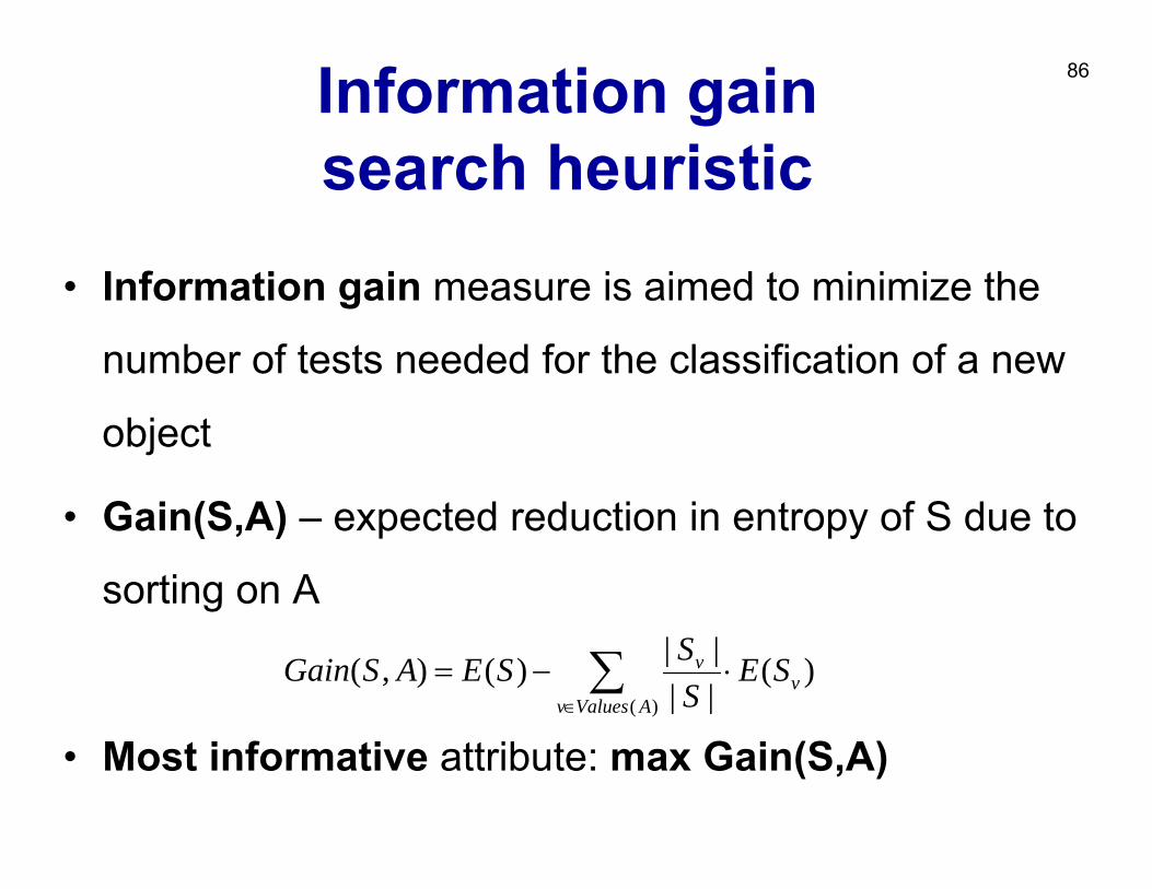
86Information gain search heuristic
• Information gain measure is aimed to minimize the
number of tests needed for the classification of a new
object
• Gain(S,A) – expected reduction in entropy of S due to
sorting on A
• Most informative attribute: max Gain(S,A)
)(||||)(),(
)(v
AValuesv
v SESSSEASGain ⋅−= ∑
∈
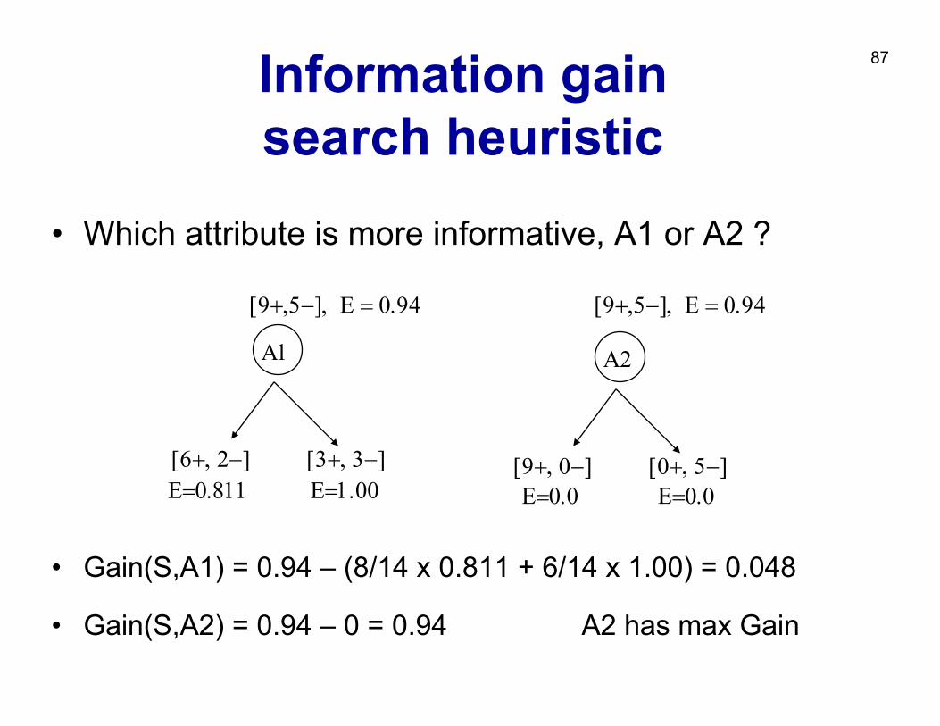
87Information gain search heuristic
• Which attribute is more informative, A1 or A2 ?
• Gain(S,A1) = 0.94 – (8/14 x 0.811 + 6/14 x 1.00) = 0.048
• Gain(S,A2) = 0.94 – 0 = 0.94 A2 has max Gain
Α1
[9+,5−], Ε = 0.94
[3+, 3−][6+, 2−]Ε=0.811 Ε=1.00
Α2
[0+, 5−][9+, 0−]Ε=0.0 Ε=0.0
[9+,5−], Ε = 0.94
88
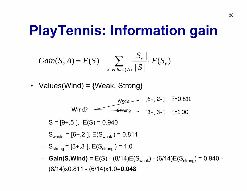
PlayTennis: Information gain
• Values(Wind) = {Weak, Strong}
– S = [9+,5-], E(S) = 0.940
– Sweak = [6+,2-], E(Sweak ) = 0.811
– Sstrong = [3+,3-], E(Sstrong ) = 1.0
– Gain(S,Wind) = E(S) - (8/14)E(Sweak) - (6/14)E(Sstrong) = 0.940 -
(8/14)x0.811 - (6/14)x1.0=0.048
)(||||)(),(
)(v
AValuesv
v SESSSEASGain ⋅−= ∑
∈
Wind?
[6+, 2-] E=0.811
[3+, 3-] E=1.00
Weak
Strong
89
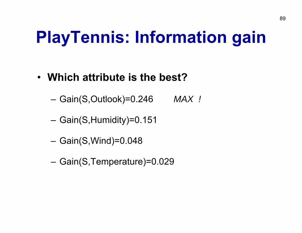
PlayTennis: Information gain
• Which attribute is the best?
– Gain(S,Outlook)=0.246 MAX !
– Gain(S,Humidity)=0.151
– Gain(S,Wind)=0.048
– Gain(S,Temperature)=0.029
90
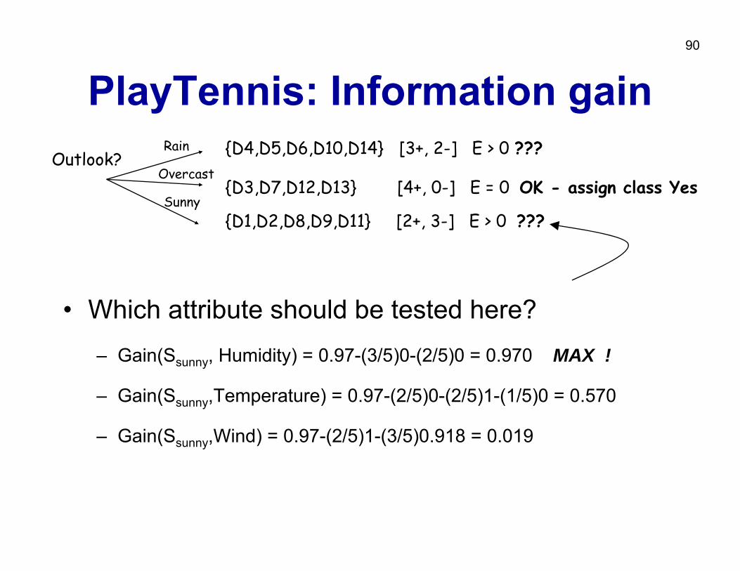
PlayTennis: Information gain
• Which attribute should be tested here?– Gain(Ssunny, Humidity) = 0.97-(3/5)0-(2/5)0 = 0.970 MAX !
– Gain(Ssunny,Temperature) = 0.97-(2/5)0-(2/5)1-(1/5)0 = 0.570
– Gain(Ssunny,Wind) = 0.97-(2/5)1-(3/5)0.918 = 0.019
Outlook?
{D1,D2,D8,D9,D11} [2+, 3-] E > 0 ???
{D3,D7,D12,D13} [4+, 0-] E = 0 OK - assign class YesSunny
Overcast
{D4,D5,D6,D10,D14} [3+, 2-] E > 0 ???Rain

91
Probability estimates• Relative frequency :
– problems with small samples
• Laplace estimate : – assumes uniform prior
distribution of k classes
)().(
)|(
CondnCondClassn
CondClassp
=
=
kCondnCondClassn
++
=)(
1).( 2=k
[6+,1-] (7) = 6/7[2+,0-] (2) = 2/2 = 1
[6+,1-] (7) = 6+1 / 7+2 = 7/9[2+,0-] (2) = 2+1 / 2+2 = 3/4
92
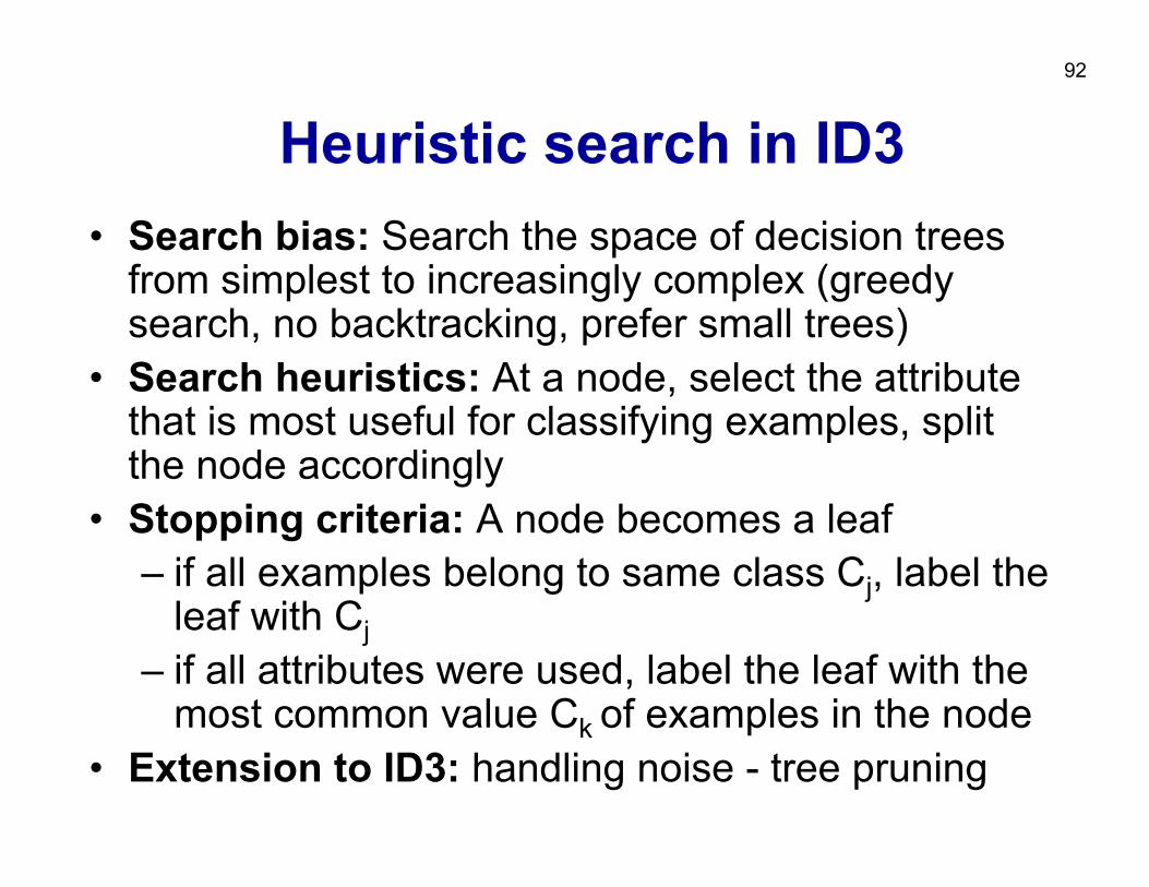
Heuristic search in ID3• Search bias: Search the space of decision trees
from simplest to increasingly complex (greedy search, no backtracking, prefer small trees)
• Search heuristics: At a node, select the attribute that is most useful for classifying examples, split the node accordingly
• Stopping criteria: A node becomes a leaf– if all examples belong to same class Cj, label the
leaf with Cj– if all attributes were used, label the leaf with the
most common value Ck of examples in the node• Extension to ID3: handling noise - tree pruning
93
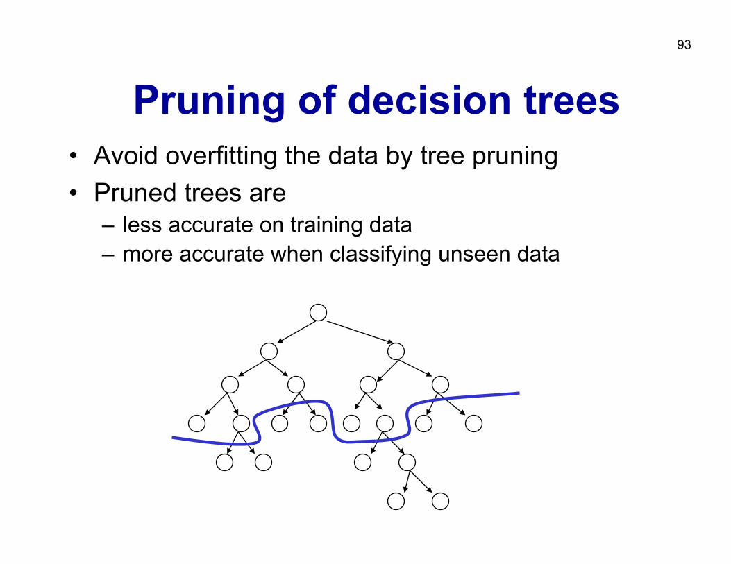
Pruning of decision trees• Avoid overfitting the data by tree pruning• Pruned trees are
– less accurate on training data– more accurate when classifying unseen data
94
Handling noise – Tree pruning
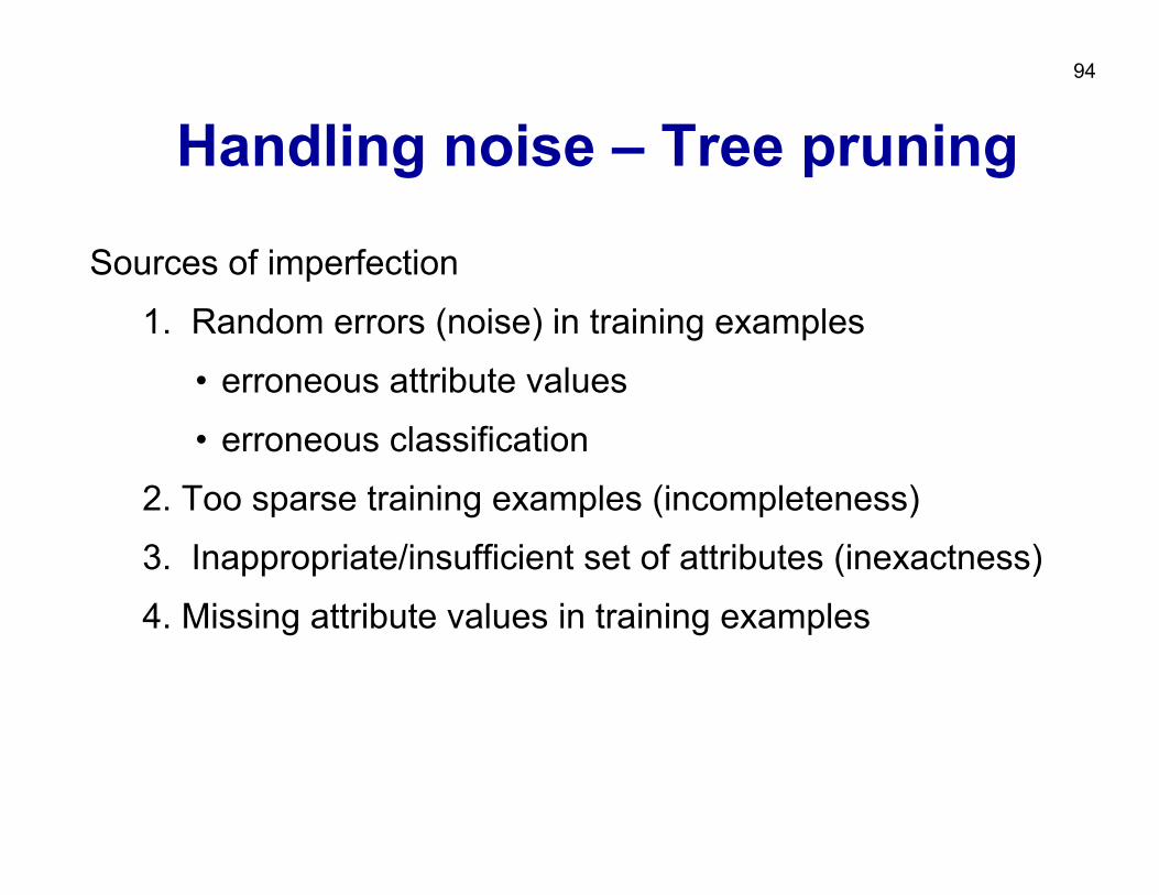
Sources of imperfection
1. Random errors (noise) in training examples
• erroneous attribute values
• erroneous classification
2. Too sparse training examples (incompleteness)
3. Inappropriate/insufficient set of attributes (inexactness)
4. Missing attribute values in training examples
95
Handling noise – Tree pruning
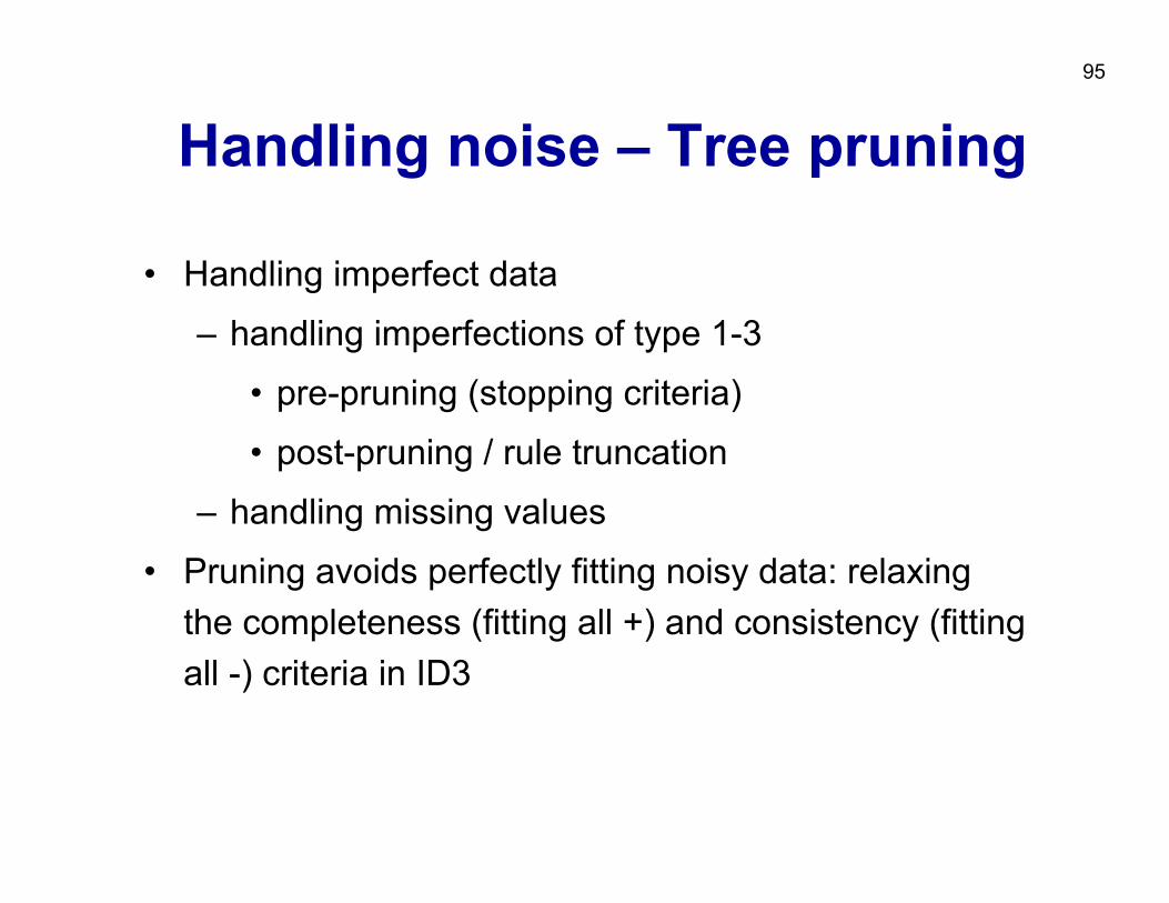
• Handling imperfect data
– handling imperfections of type 1-3
• pre-pruning (stopping criteria)
• post-pruning / rule truncation
– handling missing values
• Pruning avoids perfectly fitting noisy data: relaxing the completeness (fitting all +) and consistency (fitting all -) criteria in ID3
96
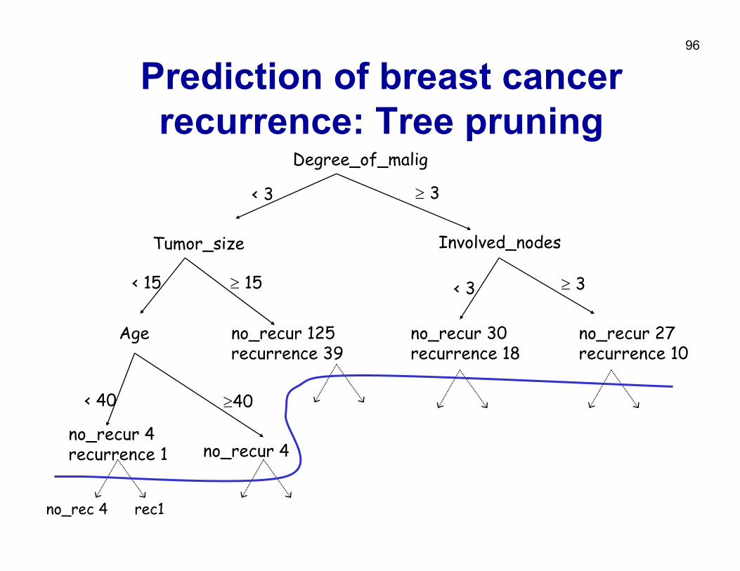
Prediction of breast cancer recurrence: Tree pruning
Degree_of_malig
Tumor_size
Age no_recur 125recurrence 39
no_recur 4recurrence 1 no_recur 4
Involved_nodes
no_recur 30recurrence 18
no_recur 27recurrence 10
< 3 ≥ 3
< 15 ≥ 15 < 3 ≥ 3
< 40 ≥40
no_rec 4 rec1
97
Accuracy and error• Accuracy: percentage of correct classifications
– on the training set– on unseen instances
• How accurate is a decision tree when classifying unseen instances– An estimate of accuracy on unseen instances can be computed,
e.g., by averaging over 4 runs:• split the example set into training set (e.g. 70%) and test set (e.g. 30%) • induce a decision tree from training set, compute its accuracy on test
set
• Error = 1 - Accuracy• High error may indicate data overfitting
98
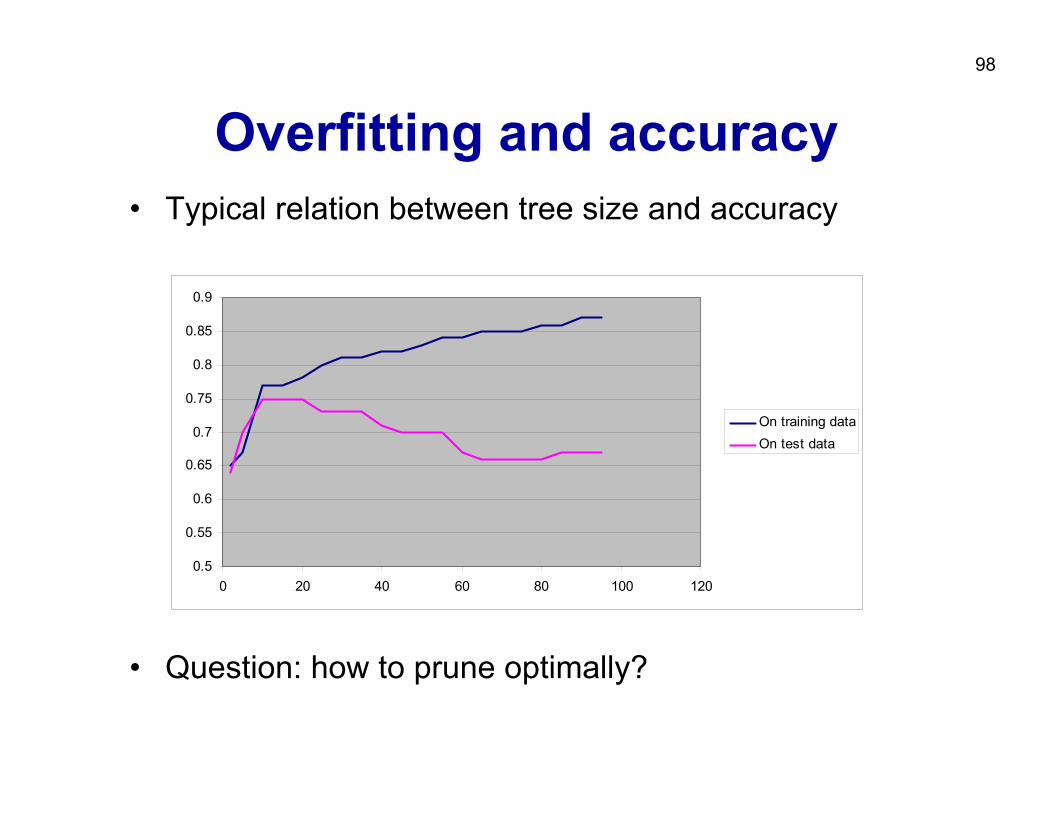
Overfitting and accuracy• Typical relation between tree size and accuracy
• Question: how to prune optimally?
0.5
0.55
0.6
0.65
0.7
0.75
0.8
0.85
0.9
0 20 40 60 80 100 120
On training dataOn test data
99
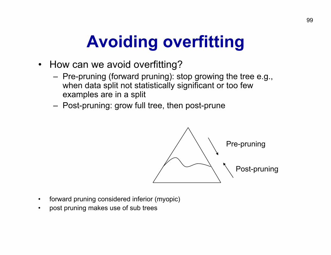
Avoiding overfitting• How can we avoid overfitting?
– Pre-pruning (forward pruning): stop growing the tree e.g., when data split not statistically significant or too few examples are in a split
– Post-pruning: grow full tree, then post-prune
• forward pruning considered inferior (myopic)• post pruning makes use of sub trees
Pre-pruning
Post-pruning
100
How to select the “best” tree• Measure performance over training data (e.g.,
pessimistic post-pruning, Quinlan 1993)• Measure performance over separate validation data
set (e.g., reduced error pruning, Quinlan 1987) – until further pruning is harmful DO:
• for each node evaluate the impact of replacing a subtree by a leaf, assigning the majority class of examples in the leaf, if the pruned tree performs no worse than the original over the validation set
• greedily select the node whose removal most improves tree accuracy over the validation set
• MDL: minimizesize(tree)+size(misclassifications(tree))
101
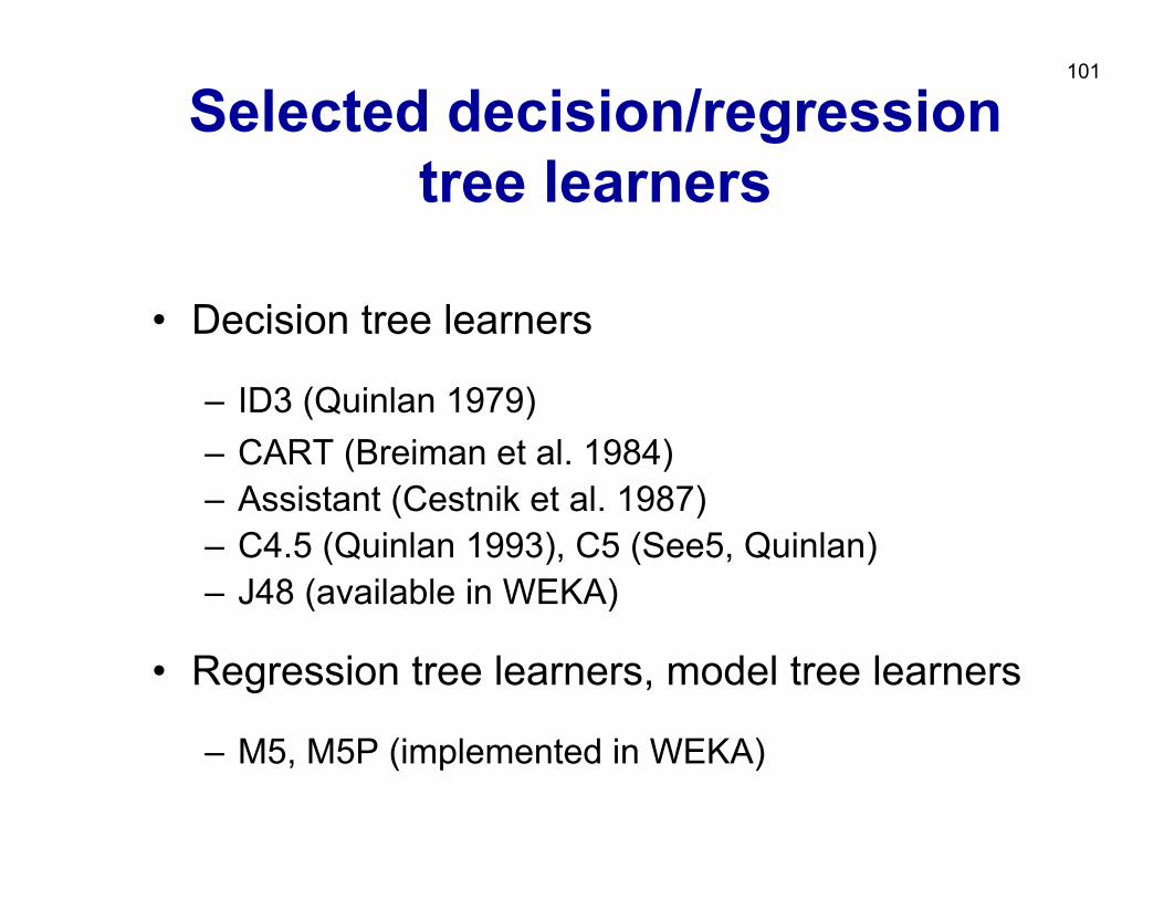
Selected decision/regression tree learners
• Decision tree learners
– ID3 (Quinlan 1979)– CART (Breiman et al. 1984)– Assistant (Cestnik et al. 1987)– C4.5 (Quinlan 1993), C5 (See5, Quinlan)– J48 (available in WEKA)
• Regression tree learners, model tree learners
– M5, M5P (implemented in WEKA)
102
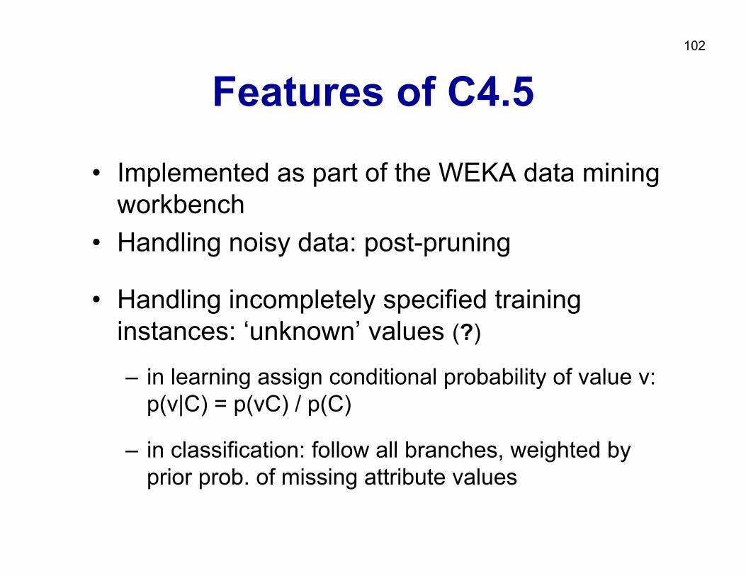
Features of C4.5
• Implemented as part of the WEKA data mining workbench
• Handling noisy data: post-pruning
• Handling incompletely specified training instances: ‘unknown’ values (?)
– in learning assign conditional probability of value v: p(v|C) = p(vC) / p(C)
– in classification: follow all branches, weighted by prior prob. of missing attribute values
103
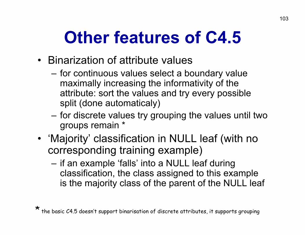
Other features of C4.5• Binarization of attribute values
– for continuous values select a boundary value maximally increasing the informativity of the attribute: sort the values and try every possible split (done automaticaly)
– for discrete values try grouping the values until two groups remain *
• ‘Majority’ classification in NULL leaf (with no corresponding training example)– if an example ‘falls’ into a NULL leaf during
classification, the class assigned to this example is the majority class of the parent of the NULL leaf
* the basic C4.5 doesn’t support binarisation of discrete attributes, it supports grouping
104
Part II. Predictive DM techniques
• Naïve Bayesian classifier• Decision tree learning• Classification rule learning• Classifier evaluation
105
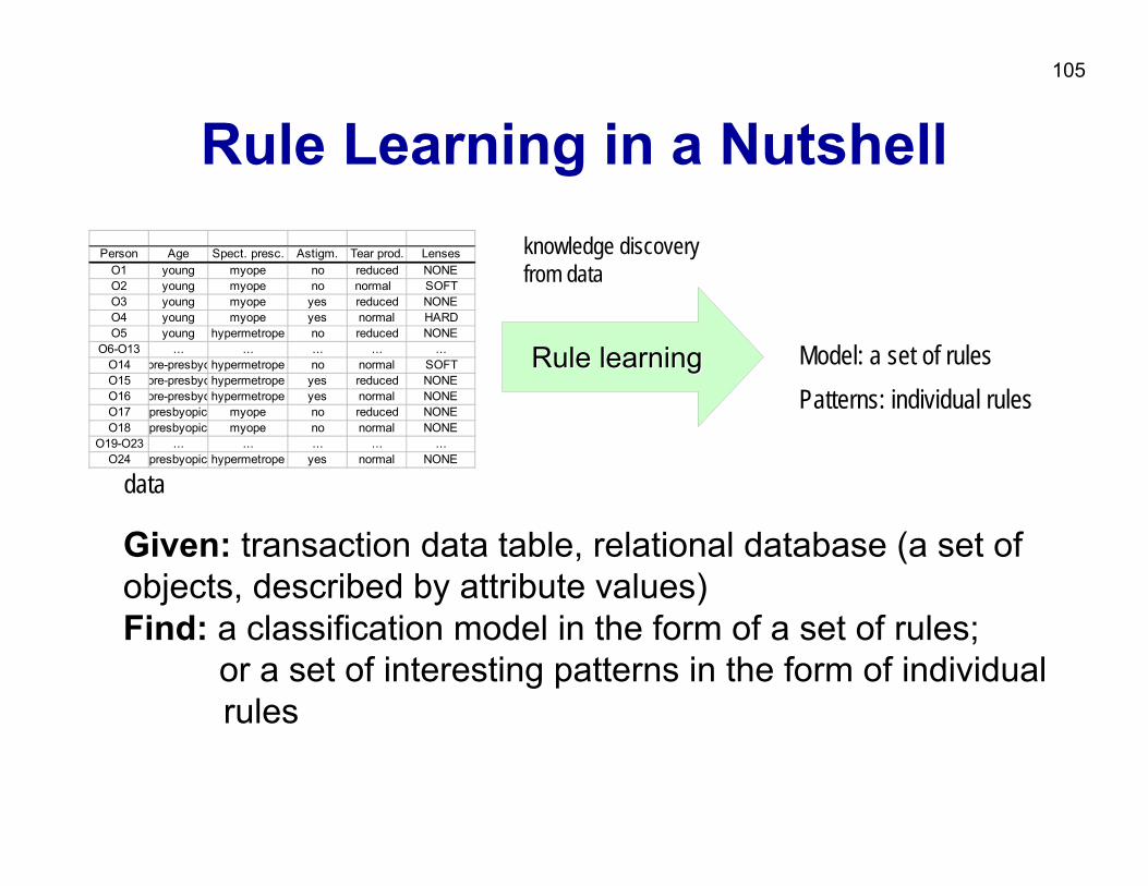
Rule Learning in a Nutshell
data
RuleRule learninglearning
knowledge discoveryfrom data
Model: a set of rulesPatterns: individual rules
Given: transaction data table, relational database (a set ofobjects, described by attribute values)Find: a classification model in the form of a set of rules;
or a set of interesting patterns in the form of individualrules
Person Age Spect. presc. Astigm. Tear prod. LensesO1 young myope no reduced NONEO2 young myope no normal SOFTO3 young myope yes reduced NONEO4 young myope yes normal HARDO5 young hypermetrope no reduced NONE
O6-O13 ... ... ... ... ...O14 pre-presbyohypermetrope no normal SOFTO15 pre-presbyohypermetrope yes reduced NONEO16 pre-presbyohypermetrope yes normal NONEO17 presbyopic myope no reduced NONEO18 presbyopic myope no normal NONE
O19-O23 ... ... ... ... ...O24 presbyopic hypermetrope yes normal NONE
106
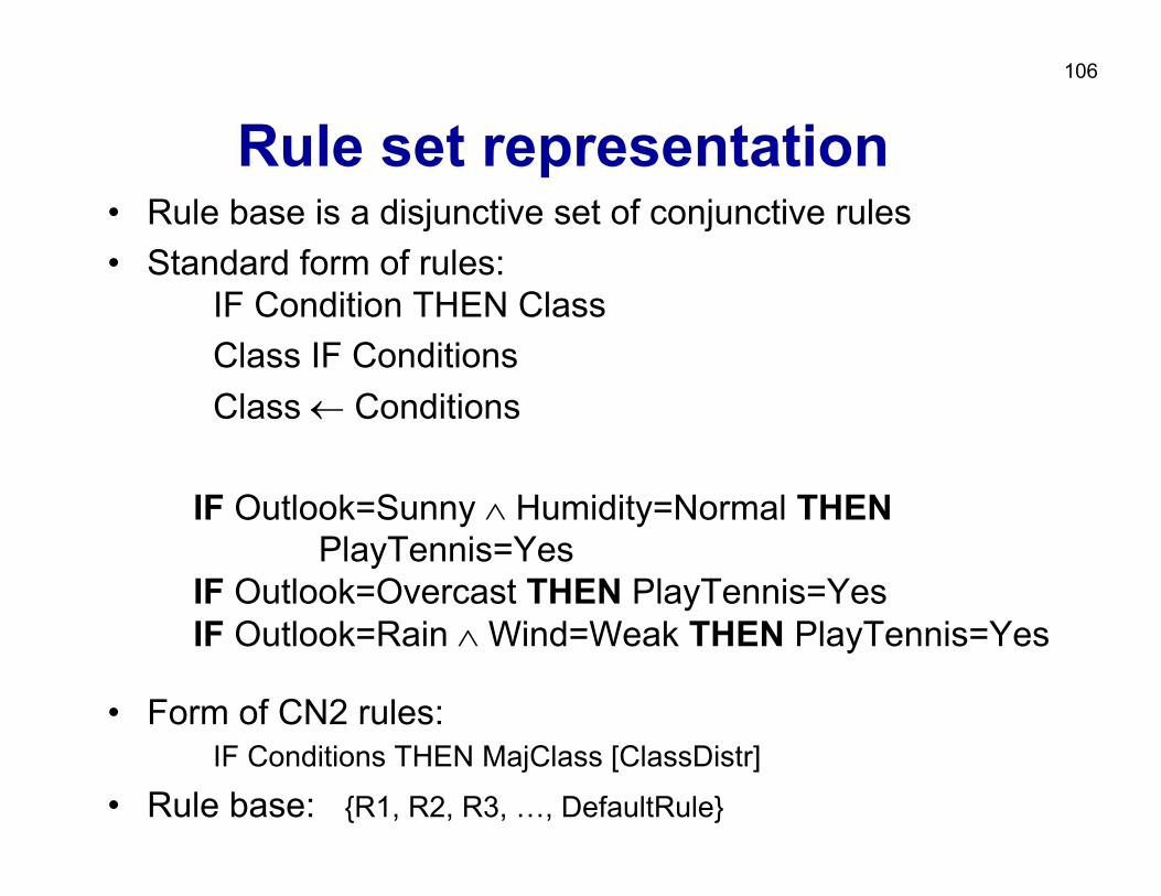
Rule set representation• Rule base is a disjunctive set of conjunctive rules• Standard form of rules:
IF Condition THEN ClassClass IF ConditionsClass ← Conditions
IF Outlook=Sunny ∧ Humidity=Normal THEN PlayTennis=Yes
IF Outlook=Overcast THEN PlayTennis=YesIF Outlook=Rain ∧ Wind=Weak THEN PlayTennis=Yes
• Form of CN2 rules: IF Conditions THEN MajClass [ClassDistr]
• Rule base: {R1, R2, R3, …, DefaultRule}

107
Data mining exampleInput: Contact lens data
Person Age Spect. presc. Astigm. Tear prod. LensesO1 young myope no reduced NONEO2 young myope no normal SOFTO3 young myope yes reduced NONEO4 young myope yes normal HARDO5 young hypermetrope no reduced NONE
O6-O13 ... ... ... ... ...O14 pre-presbyohypermetrope no normal SOFTO15 pre-presbyohypermetrope yes reduced NONEO16 pre-presbyohypermetrope yes normal NONEO17 presbyopic myope no reduced NONEO18 presbyopic myope no normal NONE
O19-O23 ... ... ... ... ...O24 presbyopic hypermetrope yes normal NONE

108
Contact lens data: Classification rules
Type of task: prediction and classificationHypothesis language: rules X C, if X then C
X conjunction of attribute values, C class
tear production=reduced → lenses=NONEtear production=normal & astigmatism=yes &
spect. pre.=hypermetrope → lenses=NONEtear production=normal & astigmatism=no →lenses=SOFTtear production=normal & astigmatism=yes &
spect. pre.=myope → lenses=HARDDEFAULT lenses=NONE
109
Rule learning• Two rule learning approaches:
– Learn decision tree, convert to rules– Learn set/list of rules
• Learning an unordered set of rules• Learning an ordered list of rules
• Heuristics, overfitting, pruning
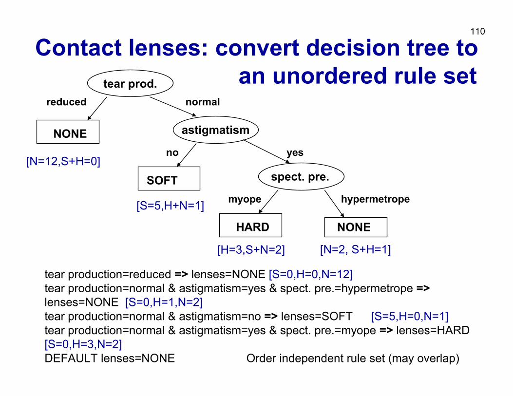
110
Contact lenses: convert decision tree to an unordered rule settear prod.
astigmatism
spect. pre.
NONE
NONE
reduced
no yes
normal
hypermetrope
SOFTmyope
HARD
[N=12,S+H=0]
[N=2, S+H=1]
[S=5,H+N=1]
[H=3,S+N=2]
tear production=reduced => lenses=NONE [S=0,H=0,N=12] tear production=normal & astigmatism=yes & spect. pre.=hypermetrope =>lenses=NONE [S=0,H=1,N=2]tear production=normal & astigmatism=no => lenses=SOFT [S=5,H=0,N=1]tear production=normal & astigmatism=yes & spect. pre.=myope => lenses=HARD [S=0,H=3,N=2]DEFAULT lenses=NONE Order independent rule set (may overlap)
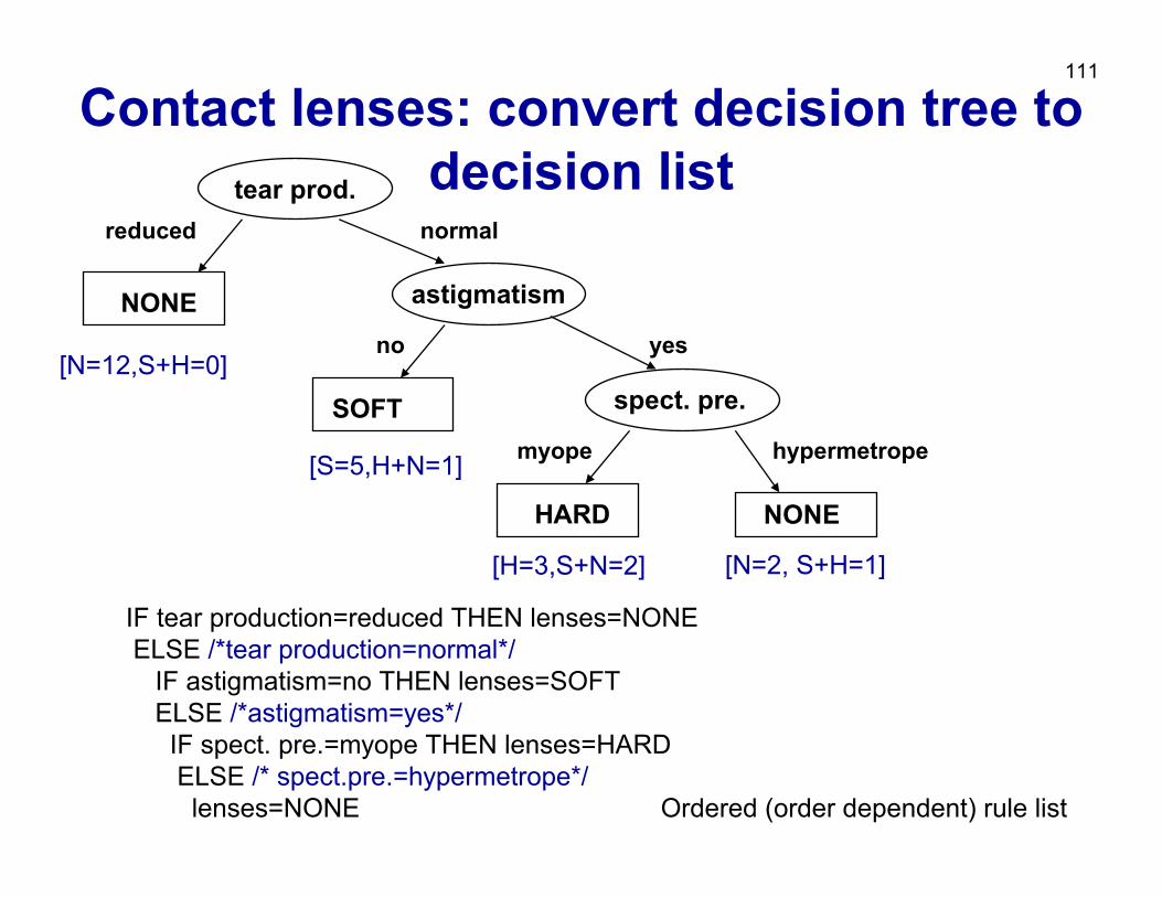
111
Contact lenses: convert decision tree to decision listtear prod.
astigmatism
spect. pre.
NONE
NONE
reduced
no yes
normal
hypermetrope
SOFTmyope
HARD
[N=12,S+H=0]
[N=2, S+H=1]
[S=5,H+N=1]
[H=3,S+N=2]
IF tear production=reduced THEN lenses=NONEELSE /*tear production=normal*/
IF astigmatism=no THEN lenses=SOFTELSE /*astigmatism=yes*/
IF spect. pre.=myope THEN lenses=HARD ELSE /* spect.pre.=hypermetrope*/
lenses=NONE Ordered (order dependent) rule list
112
Converting decision tree to rules, andrule post-pruning (Quinlan 1993)
• Very frequently used method, e.g., in C4.5and J48
• Procedure:– grow a full tree (allowing overfitting)– convert the tree to an equivalent set of rules– prune each rule independently of others– sort final rules into a desired sequence for use
113
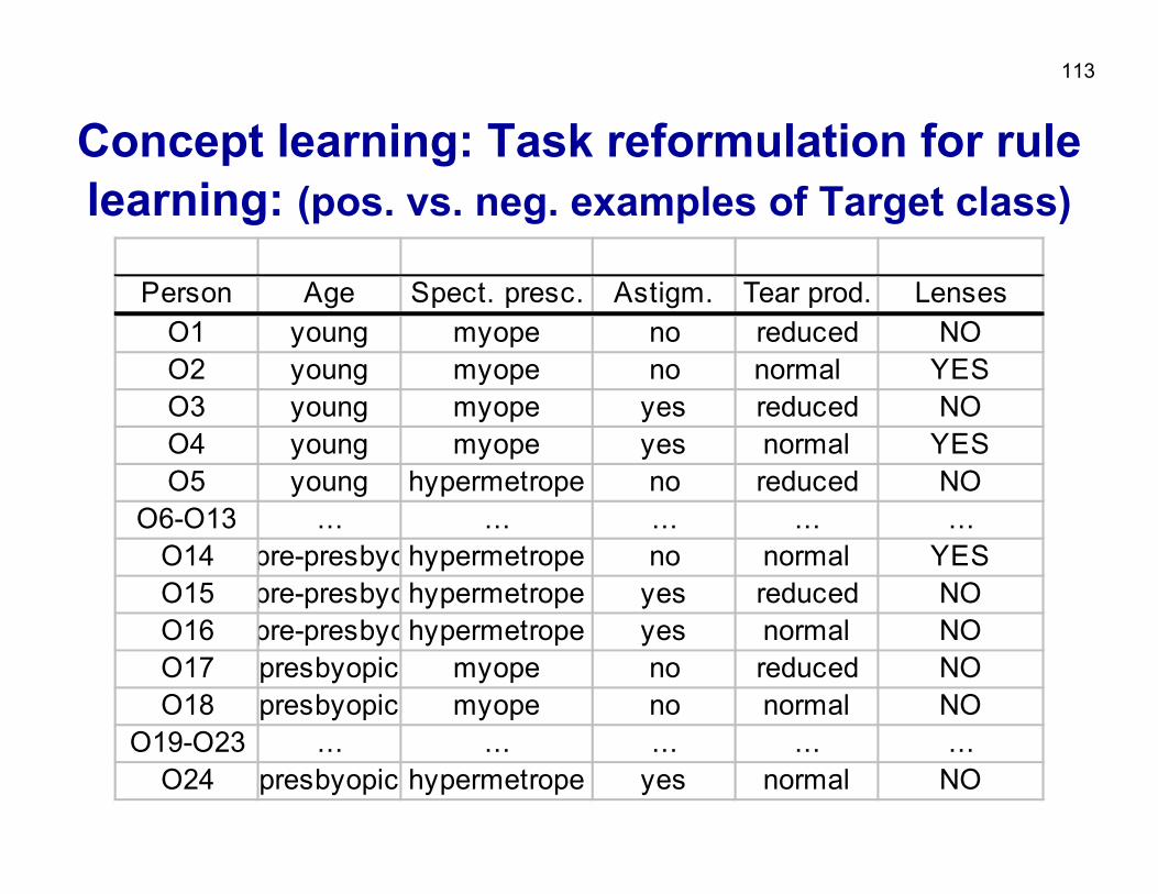
Concept learning: Task reformulation for rulelearning: (pos. vs. neg. examples of Target class)
Person Age Spect. presc. Astigm. Tear prod. LensesO1 young myope no reduced NOO2 young myope no normal YESO3 young myope yes reduced NOO4 young myope yes normal YESO5 young hypermetrope no reduced NO
O6-O13 ... ... ... ... ...O14 pre-presbyohypermetrope no normal YESO15 pre-presbyohypermetrope yes reduced NOO16 pre-presbyohypermetrope yes normal NOO17 presbyopic myope no reduced NOO18 presbyopic myope no normal NO
O19-O23 ... ... ... ... ...O24 presbyopic hypermetrope yes normal NO
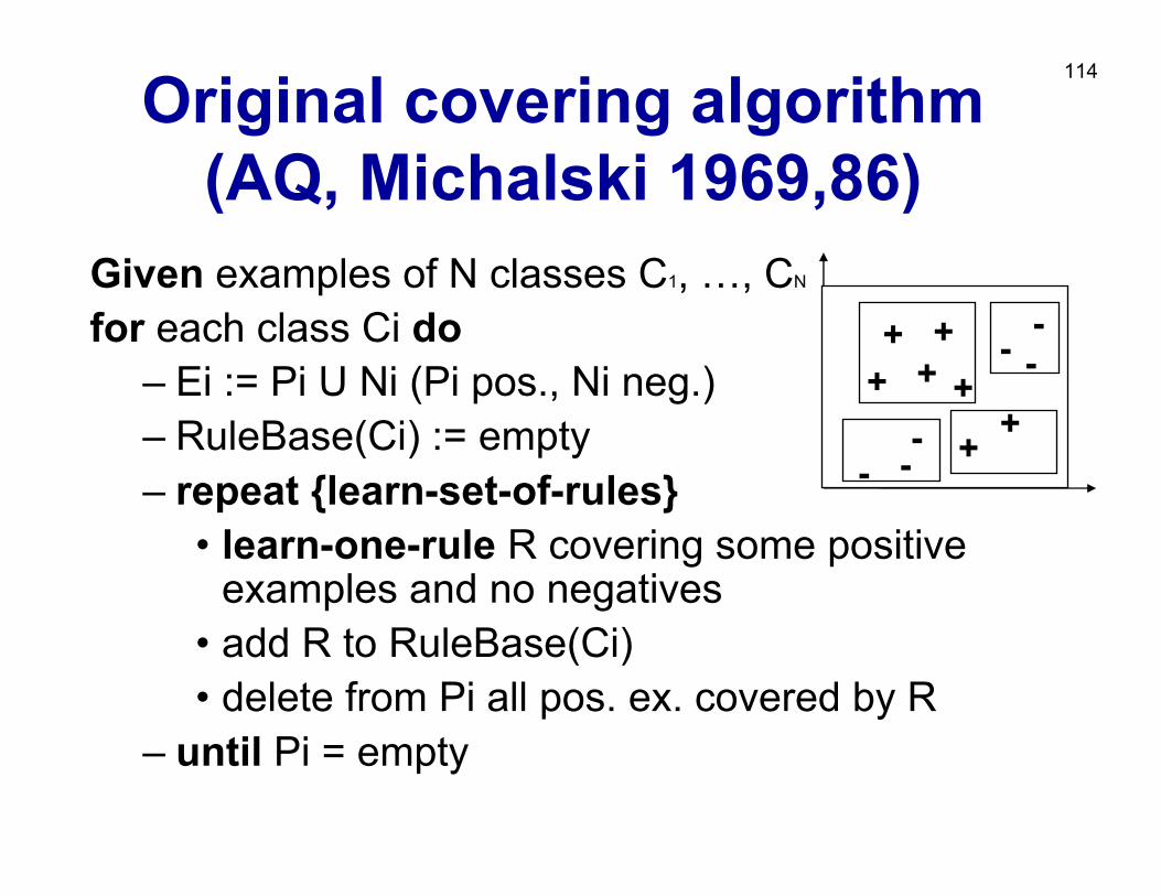
114Original covering algorithm(AQ, Michalski 1969,86)
Given examples of N classes C1, …, CN
for each class Ci do– Ei := Pi U Ni (Pi pos., Ni neg.)– RuleBase(Ci) := empty– repeat {learn-set-of-rules}
• learn-one-rule R covering some positive examples and no negatives
• add R to RuleBase(Ci)• delete from Pi all pos. ex. covered by R
– until Pi = empty
++
++ +
+-
--
--
+-
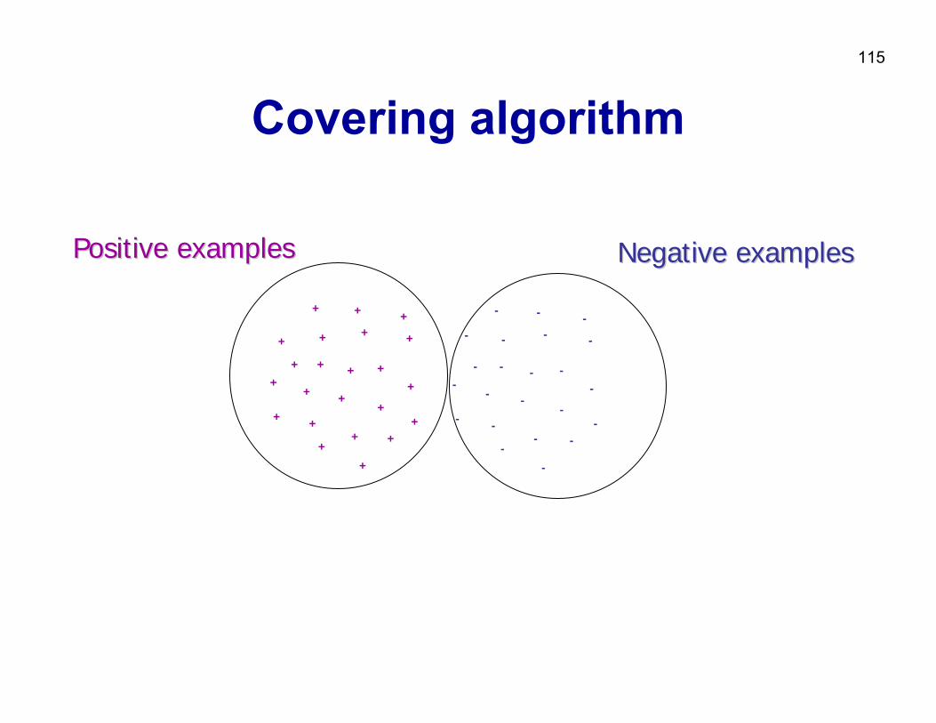
115
Covering algorithm
+ +
+
+
+
+
+
+
+
++ +
++
+
+
++
+
++
+
+
- -
-
-
-
-
-
-
-
--
--
-
-
--
-
--
-
-
PositivePositive examplesexamples NNegativeegative examplesexamples
-
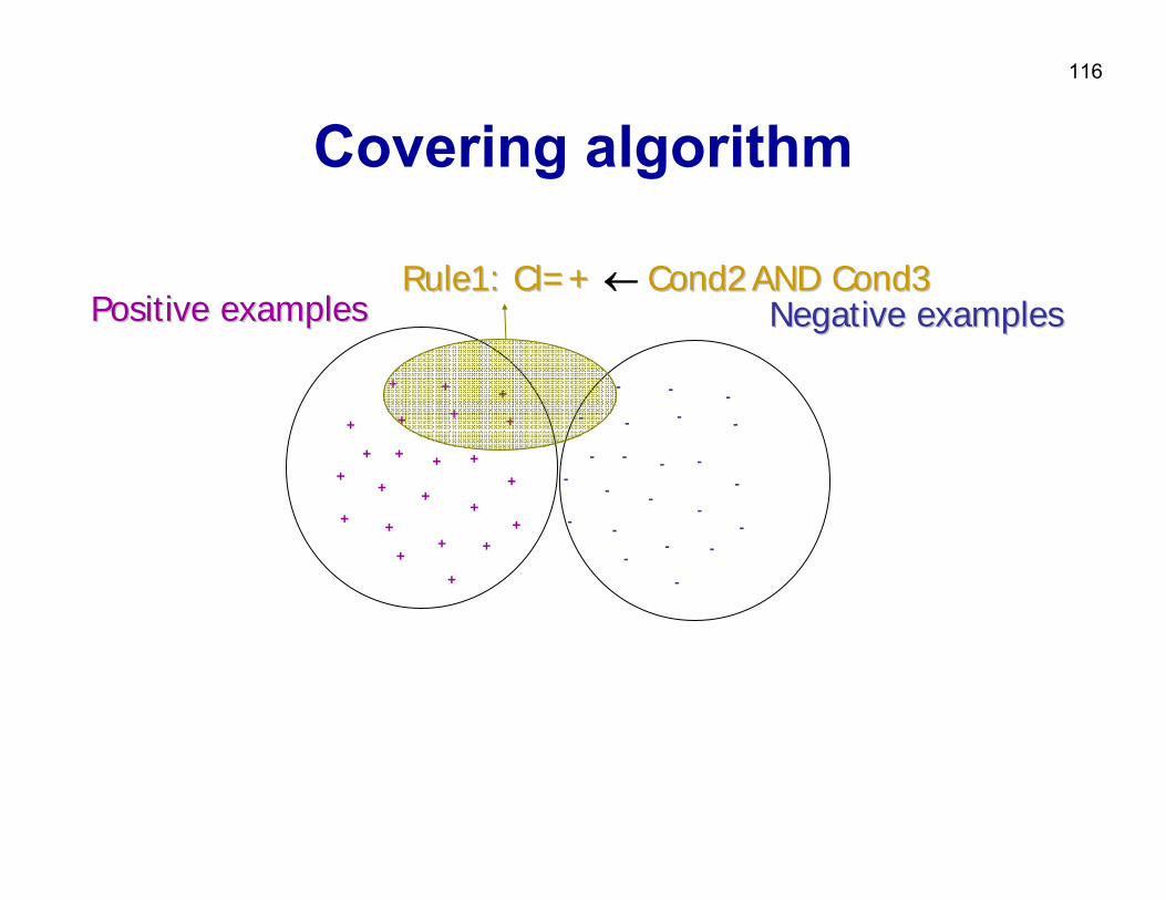
116
Covering algorithm
+ +
+
+
+
+
+
+
+
++ +
++
+
+
++
+
++
+
+
- -
-
-
-
-
-
-
-
--
--
-
-
--
-
--
-
-
PositivePositive examplesexamples NNegativeegative examplesexamples
-
Rule1: Rule1: ClCl=+ =+ ← Cond2Cond2 AND Cond3AND Cond3

117
Covering algorithm
++
+
+
+
+
++
+
+
++
+
++
+
+
- -
-
-
-
-
-
-
-
--
--
-
-
--
-
--
-
-
PositivePositive examplesexamples NNegativeegative examplesexamples
-
Rule1: Rule1: ClCl=+ =+ ← Cond2Cond2 AND Cond3AND Cond3

118
Covering algorithm
++
+
+
+
+
++
+
+
++
+
++
+
+
- -
-
-
-
-
-
-
-
--
--
-
-
--
-
--
-
-
PositivePositive examplesexamples NNegativeegative examplesexamples
-
Rule1: Rule1: ClCl=+ =+ ← Cond2 AND Cond3Cond2 AND Cond3
Rule2: Rule2: ClCl=+ =+ ← Cond8Cond8 AND Cond6AND Cond6
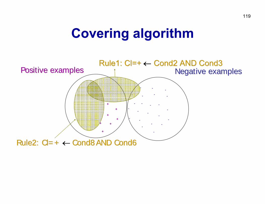
119
Covering algorithm
+
+
+
+
++
+
- -
-
-
-
-
-
-
-
--
--
-
-
--
-
--
-
-
PositivePositive examplesexamples NNegativeegative examplesexamples
-
Rule1: Rule1: ClCl=+ =+ ← Cond2 AND Cond3Cond2 AND Cond3
Rule2: Rule2: ClCl=+ =+ ← Cond8Cond8 AND Cond6AND Cond6
120
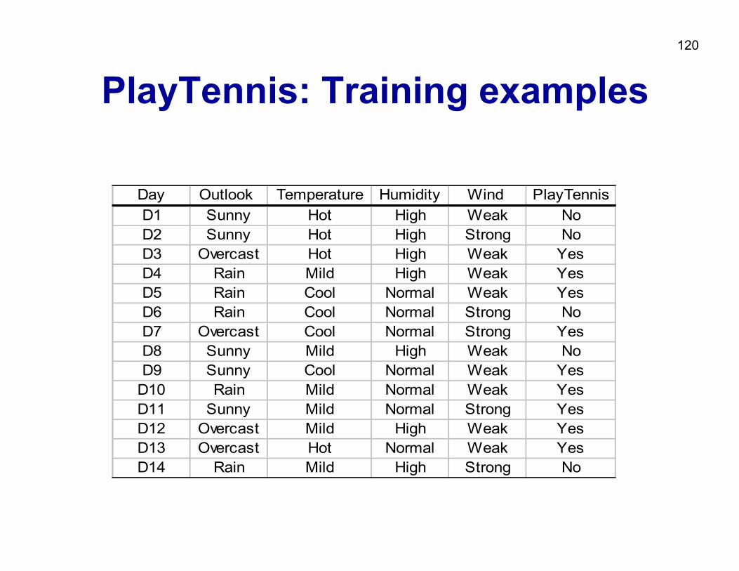
PlayTennis: Training examples
Day Outlook Temperature Humidity Wind PlayTennisD1 Sunny Hot High Weak NoD2 Sunny Hot High Strong NoD3 Overcast Hot High Weak YesD4 Rain Mild High Weak YesD5 Rain Cool Normal Weak YesD6 Rain Cool Normal Strong NoD7 Overcast Cool Normal Strong YesD8 Sunny Mild High Weak NoD9 Sunny Cool Normal Weak Yes
D10 Rain Mild Normal Weak YesD11 Sunny Mild Normal Strong YesD12 Overcast Mild High Weak YesD13 Overcast Hot Normal Weak YesD14 Rain Mild High Strong No
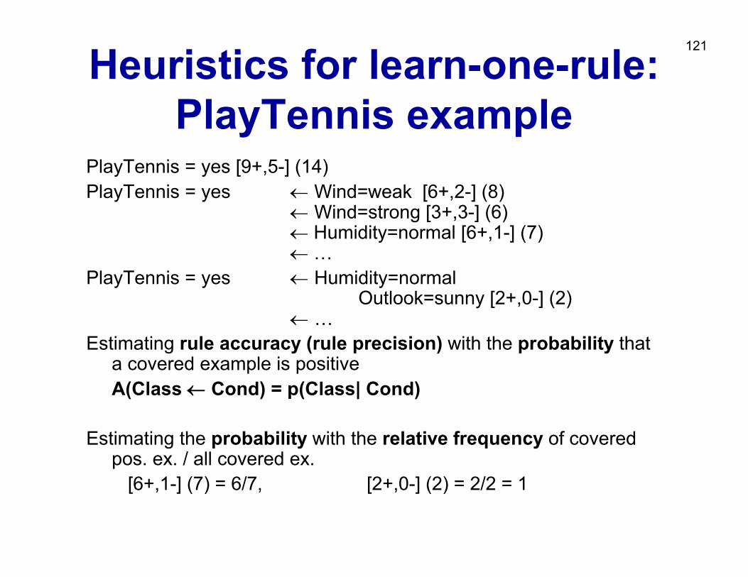
121Heuristics for learn-one-rule:PlayTennis example
PlayTennis = yes [9+,5-] (14)PlayTennis = yes ← Wind=weak [6+,2-] (8)
← Wind=strong [3+,3-] (6) ← Humidity=normal [6+,1-] (7)← …
PlayTennis = yes ← Humidity=normalOutlook=sunny [2+,0-] (2)
← …Estimating rule accuracy (rule precision) with the probability that
a covered example is positiveA(Class ← Cond) = p(Class| Cond)
Estimating the probability with the relative frequency of covered pos. ex. / all covered ex.
[6+,1-] (7) = 6/7, [2+,0-] (2) = 2/2 = 1
122
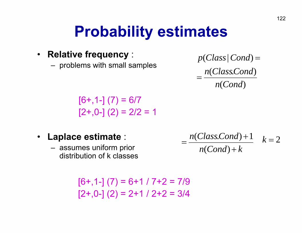
Probability estimates• Relative frequency :
– problems with small samples
• Laplace estimate : – assumes uniform prior
distribution of k classes
)().(
)|(
CondnCondClassn
CondClassp
=
=
kCondnCondClassn
++
=)(
1).( 2=k
[6+,1-] (7) = 6/7[2+,0-] (2) = 2/2 = 1
[6+,1-] (7) = 6+1 / 7+2 = 7/9[2+,0-] (2) = 2+1 / 2+2 = 3/4

123Learn-one-rule:search heuristics
• Assume a two-class problem• Two classes (+,-), learn rules for + class (Cl). • Search for specializations R’ of a rule R = Cl ← Cond
from the RuleBase.• Specializarion R’ of rule R = Cl ← Cond
has the form R’ = Cl ← Cond & Cond’• Heuristic search for rules: find the ‘best’ Cond’ to be
added to the current rule R, such that rule accuracy is improved, e.g., such that Acc(R’) > Acc(R)– where the expected classification accuracy can be
estimated as A(R) = p(Cl|Cond)
124
Learn-one-rule:Greedy vs. beam search
• learn-one-rule by greedy general-to-specific search, at each step selecting the `best’descendant, no backtracking– e.g., the best descendant of the initial rule
PlayTennis = yes ←– is rule PlayTennis = yes ← Humidity=normal
• beam search: maintain a list of k best candidates at each step; descendants (specializations) of each of these k candidates are generated, and the resulting set is again reduced to k best candidates
125
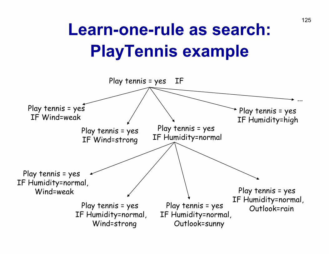
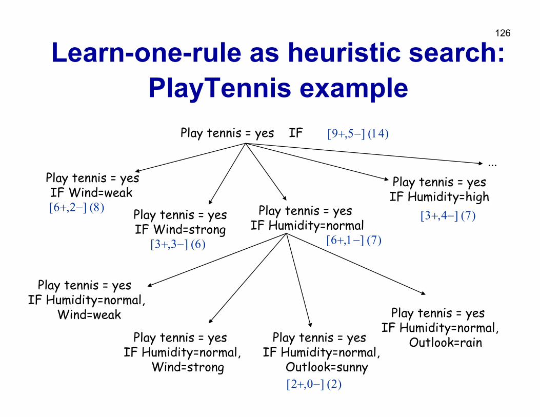
Learn-one-rule as search: PlayTennis example
Play tennis = yes IF
Play tennis = yes IF Wind=weak
Play tennis = yesIF Wind=strong
Play tennis = yes IF Humidity=normal
Play tennis = yesIF Humidity=high
Play tennis = yes IF Humidity=normal,
Wind=weak
Play tennis = yes IF Humidity=normal,
Wind=strong
Play tennis = yes IF Humidity=normal,
Outlook=sunny
Play tennis = yes IF Humidity=normal,
Outlook=rain
...
126
Learn-one-rule as heuristic search: PlayTennis example
Play tennis = yes IF
Play tennis = yes IF Wind=weak
Play tennis = yesIF Wind=strong
Play tennis = yes IF Humidity=normal
Play tennis = yesIF Humidity=high
Play tennis = yes IF Humidity=normal,
Wind=weak
Play tennis = yes IF Humidity=normal,
Wind=strong
Play tennis = yes IF Humidity=normal,
Outlook=sunny
Play tennis = yes IF Humidity=normal,
Outlook=rain
[9+,5−] (14)
[6+,2−] (8)
[3+,3−] (6) [6+,1−] (7)
[3+,4−] (7)
...
[2+,0−] (2)
127
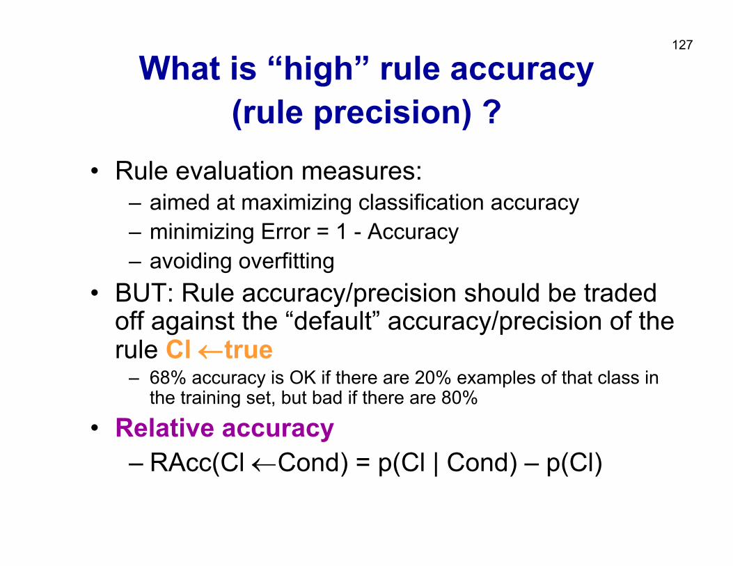
What is “high” rule accuracy(rule precision) ?
• Rule evaluation measures: – aimed at maximizing classification accuracy – minimizing Error = 1 - Accuracy– avoiding overfitting
• BUT: Rule accuracy/precision should be traded off against the “default” accuracy/precision of the rule Cl ←true
– 68% accuracy is OK if there are 20% examples of that class in the training set, but bad if there are 80%
• Relative accuracy– RAcc(Cl ←Cond) = p(Cl | Cond) – p(Cl)
128
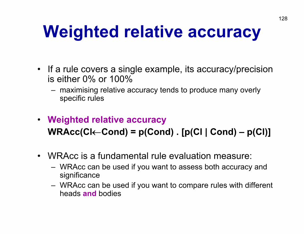
Weighted relative accuracy
• If a rule covers a single example, its accuracy/precision is either 0% or 100%– maximising relative accuracy tends to produce many overly
specific rules
• Weighted relative accuracyWRAcc(Cl←Cond) = p(Cond) . [p(Cl | Cond) – p(Cl)]
• WRAcc is a fundamental rule evaluation measure: – WRAcc can be used if you want to assess both accuracy and
significance– WRAcc can be used if you want to compare rules with different
heads and bodies
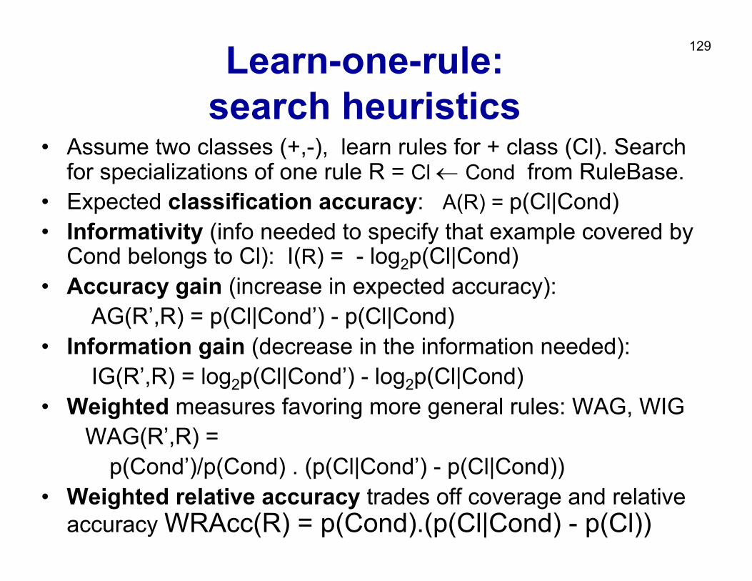
129Learn-one-rule:search heuristics
• Assume two classes (+,-), learn rules for + class (Cl). Search for specializations of one rule R = Cl ← Cond from RuleBase.
• Expected classification accuracy: A(R) = p(Cl|Cond)• Informativity (info needed to specify that example covered by
Cond belongs to Cl): I(R) = - log2p(Cl|Cond)• Accuracy gain (increase in expected accuracy):
AG(R’,R) = p(Cl|Cond’) - p(Cl|Cond)• Information gain (decrease in the information needed):
IG(R’,R) = log2p(Cl|Cond’) - log2p(Cl|Cond)• Weighted measures favoring more general rules: WAG, WIG
WAG(R’,R) = p(Cond’)/p(Cond) . (p(Cl|Cond’) - p(Cl|Cond))
• Weighted relative accuracy trades off coverage and relative accuracy WRAcc(R) = p(Cond).(p(Cl|Cond) - p(Cl))
130
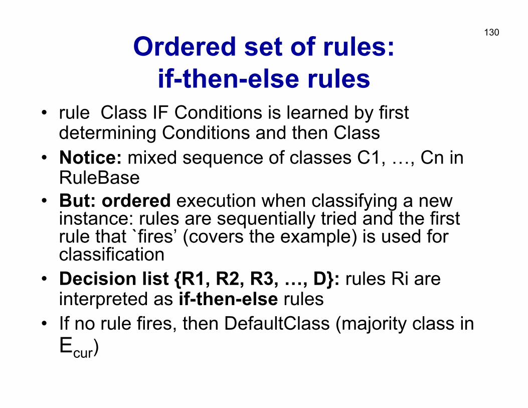
Ordered set of rules:if-then-else rules
• rule Class IF Conditions is learned by first determining Conditions and then Class
• Notice: mixed sequence of classes C1, …, Cn in RuleBase
• But: ordered execution when classifying a new instance: rules are sequentially tried and the first rule that `fires’ (covers the example) is used for classification
• Decision list {R1, R2, R3, …, D}: rules Ri are interpreted as if-then-else rules
• If no rule fires, then DefaultClass (majority class inEcur)
131
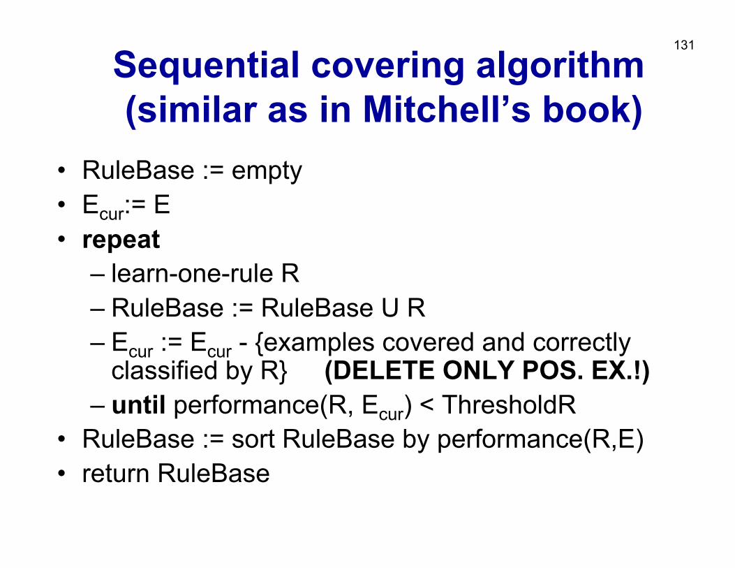
Sequential covering algorithm(similar as in Mitchell’s book)
• RuleBase := empty • Ecur:= E • repeat
– learn-one-rule R– RuleBase := RuleBase U R– Ecur := Ecur - {examples covered and correctly
classified by R} (DELETE ONLY POS. EX.!)– until performance(R, Ecur) < ThresholdR
• RuleBase := sort RuleBase by performance(R,E)• return RuleBase
132
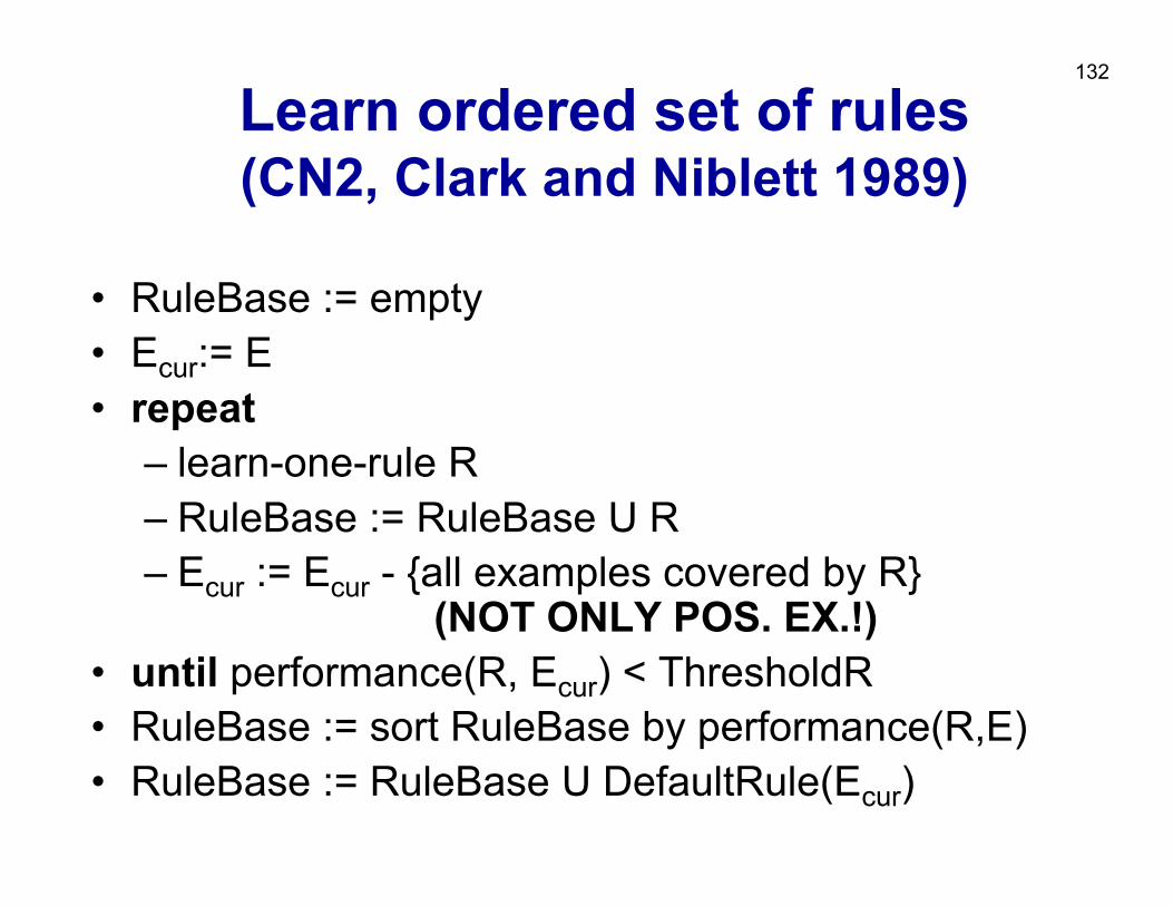
Learn ordered set of rules(CN2, Clark and Niblett 1989)
• RuleBase := empty • Ecur:= E • repeat
– learn-one-rule R– RuleBase := RuleBase U R– Ecur := Ecur - {all examples covered by R}
(NOT ONLY POS. EX.!)• until performance(R, Ecur) < ThresholdR• RuleBase := sort RuleBase by performance(R,E)• RuleBase := RuleBase U DefaultRule(Ecur)
133
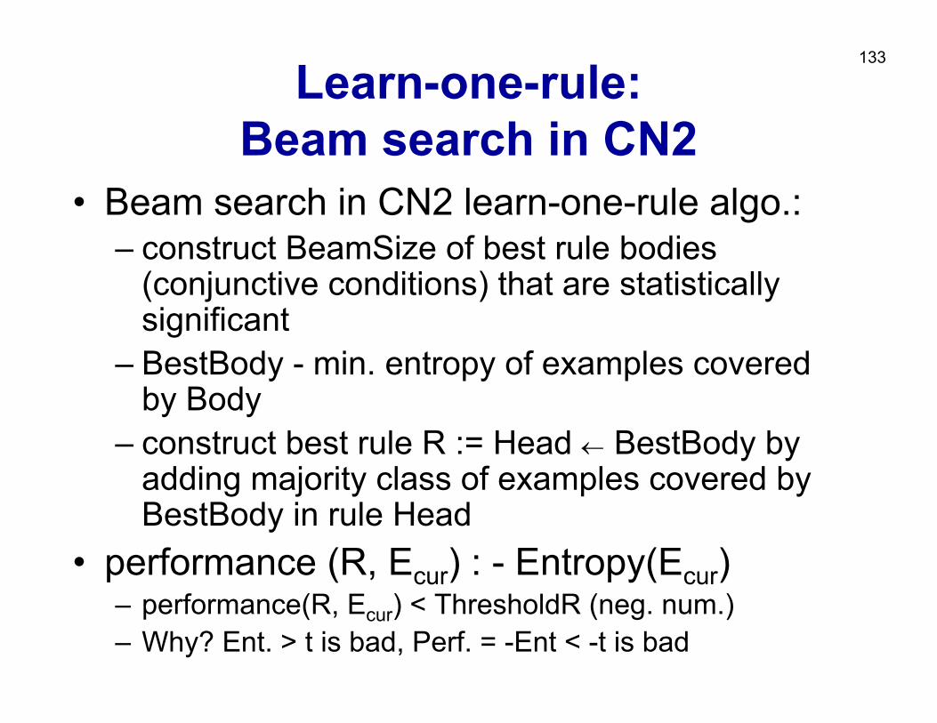
Learn-one-rule:Beam search in CN2
• Beam search in CN2 learn-one-rule algo.:– construct BeamSize of best rule bodies
(conjunctive conditions) that are statistically significant
– BestBody - min. entropy of examples covered by Body
– construct best rule R := Head ← BestBody by adding majority class of examples covered by BestBody in rule Head
• performance (R, Ecur) : - Entropy(Ecur) – performance(R, Ecur) < ThresholdR (neg. num.)– Why? Ent. > t is bad, Perf. = -Ent < -t is bad
134
Variations• Sequential vs. simultaneous covering of data (as
in TDIDT): choosing between attribute-values vs. choosing attributes
• Learning rules vs. learning decision trees and converting them to rules
• Pre-pruning vs. post-pruning of rules• What statistical evaluation functions to use• Probabilistic classification
135
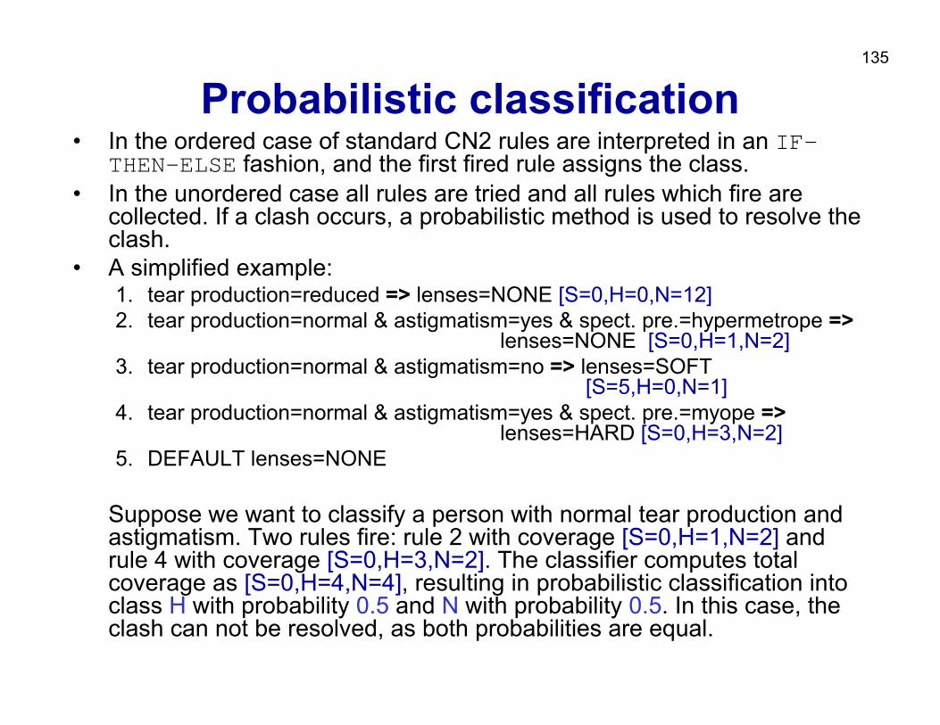
Probabilistic classification• In the ordered case of standard CN2 rules are interpreted in an IF-
THEN-ELSE fashion, and the first fired rule assigns the class.• In the unordered case all rules are tried and all rules which fire are
collected. If a clash occurs, a probabilistic method is used to resolve the clash.
• A simplified example:1. tear production=reduced => lenses=NONE [S=0,H=0,N=12] 2. tear production=normal & astigmatism=yes & spect. pre.=hypermetrope =>
lenses=NONE [S=0,H=1,N=2]3. tear production=normal & astigmatism=no => lenses=SOFT
[S=5,H=0,N=1]4. tear production=normal & astigmatism=yes & spect. pre.=myope =>
lenses=HARD [S=0,H=3,N=2]5. DEFAULT lenses=NONE
Suppose we want to classify a person with normal tear production and astigmatism. Two rules fire: rule 2 with coverage [S=0,H=1,N=2] and rule 4 with coverage [S=0,H=3,N=2]. The classifier computes total coverage as [S=0,H=4,N=4], resulting in probabilistic classification into class H with probability 0.5 and N with probability 0.5. In this case, the clash can not be resolved, as both probabilities are equal.
136
Part II. Predictive DM techniques
• Naïve Bayesian classifier• Decision tree learning• Classification rule learning• Classifier evaluation
137
Classifier evaluation
• Accuracy and Error• n-fold cross-validation• Confusion matrix• ROC
138
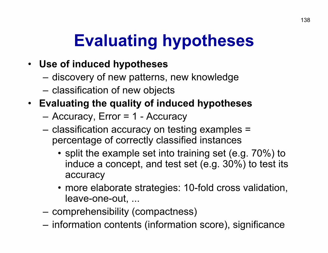
Evaluating hypotheses• Use of induced hypotheses
– discovery of new patterns, new knowledge– classification of new objects
• Evaluating the quality of induced hypotheses– Accuracy, Error = 1 - Accuracy– classification accuracy on testing examples =
percentage of correctly classified instances• split the example set into training set (e.g. 70%) to
induce a concept, and test set (e.g. 30%) to test its accuracy
• more elaborate strategies: 10-fold cross validation, leave-one-out, ...
– comprehensibility (compactness)– information contents (information score), significance
139
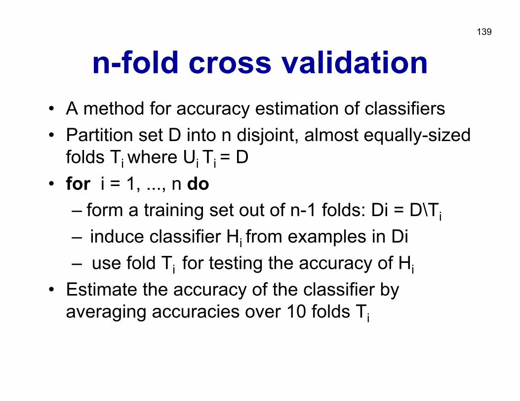
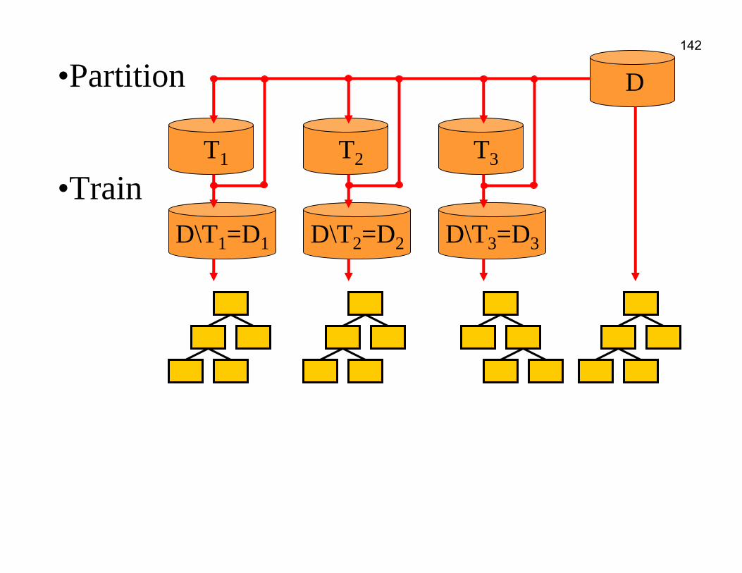
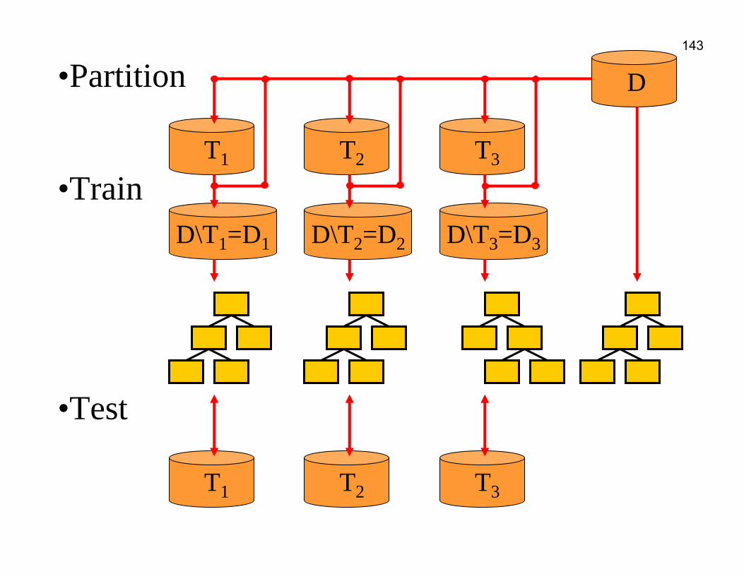
n-fold cross validation• A method for accuracy estimation of classifiers• Partition set D into n disjoint, almost equally-sized
folds Ti where Ui Ti = D• for i = 1, ..., n do
– form a training set out of n-1 folds: Di = D\Ti
– induce classifier Hi from examples in Di– use fold Ti for testing the accuracy of Hi
• Estimate the accuracy of the classifier by averaging accuracies over 10 folds Ti
140
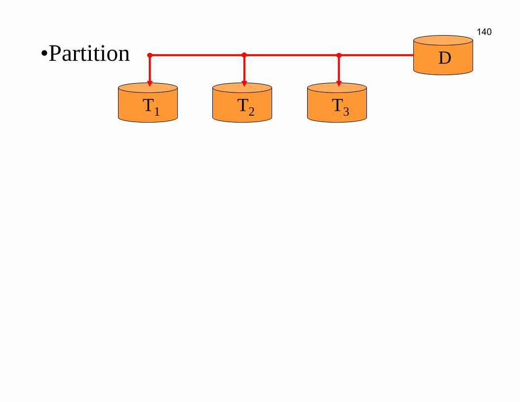
•Partition D
T1 T2 T3
141
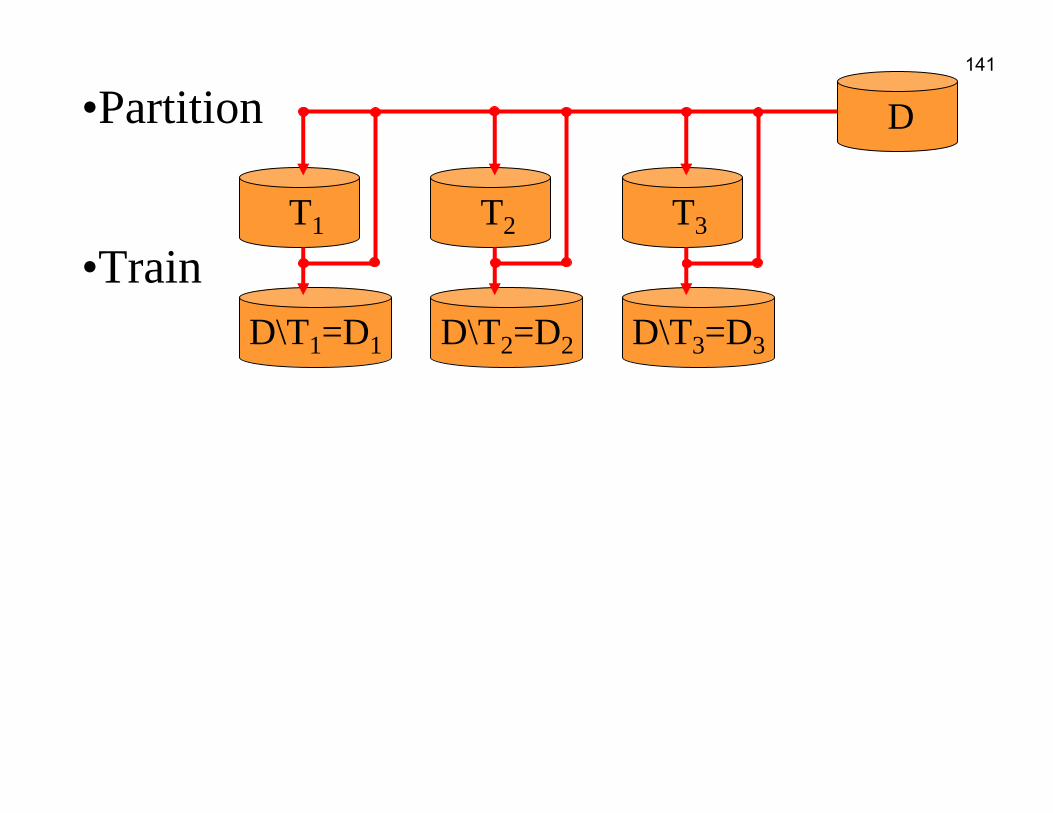
•Partition
•TrainD\T1=D1 D\T2=D2 D\T3=D3
D
T1 T2 T3
142
•Partition
•TrainD\T1=D1 D\T2=D2 D\T3=D3
D
T1 T2 T3
143
•Partition
•Train
•Test
D\T1=D1 D\T2=D2 D\T3=D3
D
T1 T2 T3
T1 T2 T3
144
Confusion matrix and rule (in)accuracy
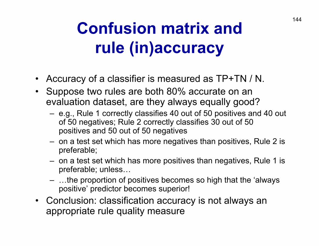
• Accuracy of a classifier is measured as TP+TN / N.• Suppose two rules are both 80% accurate on an
evaluation dataset, are they always equally good? – e.g., Rule 1 correctly classifies 40 out of 50 positives and 40 out
of 50 negatives; Rule 2 correctly classifies 30 out of 50 positives and 50 out of 50 negatives
– on a test set which has more negatives than positives, Rule 2 ispreferable;
– on a test set which has more positives than negatives, Rule 1 ispreferable; unless…
– …the proportion of positives becomes so high that the ‘always positive’ predictor becomes superior!
• Conclusion: classification accuracy is not always an appropriate rule quality measure
145
Confusion matrix
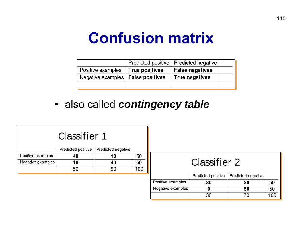
• also called contingency table
Predicted positive Predicted negative Positive examples True positives False negatives Negative examples False positives True negatives
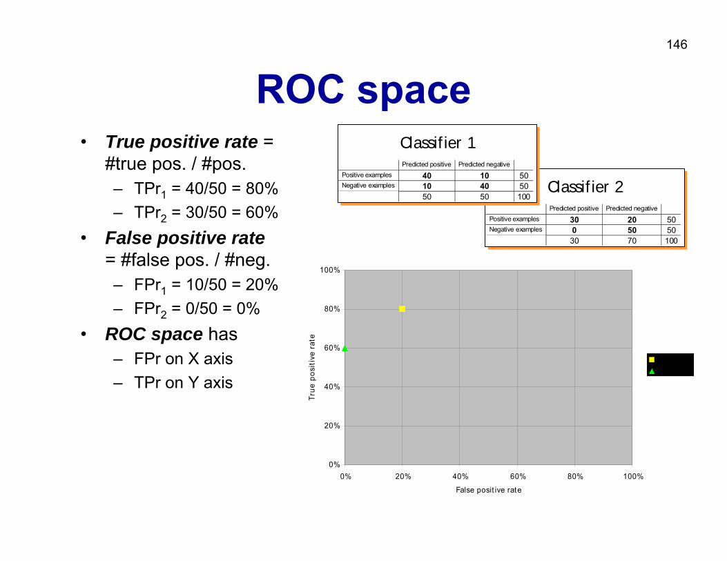
Classifier 1 Predicted positive Predicted negative Positive examples 40 10 50 Negative examples 10 40 50 50 50 100
Classifier 2 Predicted positive Predicted negative Positive examples 30 20 50 Negative examples 0 50 50 30 70 100
146
ROC space• True positive rate =
#true pos. / #pos.– TPr1 = 40/50 = 80% – TPr2 = 30/50 = 60%
• False positive rate= #false pos. / #neg.– FPr1 = 10/50 = 20%– FPr2 = 0/50 = 0%
• ROC space has – FPr on X axis – TPr on Y axis
0%
20%
40%
60%
80%
100%
0% 20% 40% 60% 80% 100%
False posit ive rate
True
pos
itive
rat
e
classif ier 1classif ier 2
Classifier 2Predicted positive Predicted negative
Positive examples 30 20 50Negative examples 0 50 50
30 70 100
Classifier 1Predicted positive Predicted negative
Positive examples 40 10 50Negative examples 10 40 50
50 50 100
147
0%
20%
40%
60%
80%
100%
0% 20% 40% 60% 80% 100%
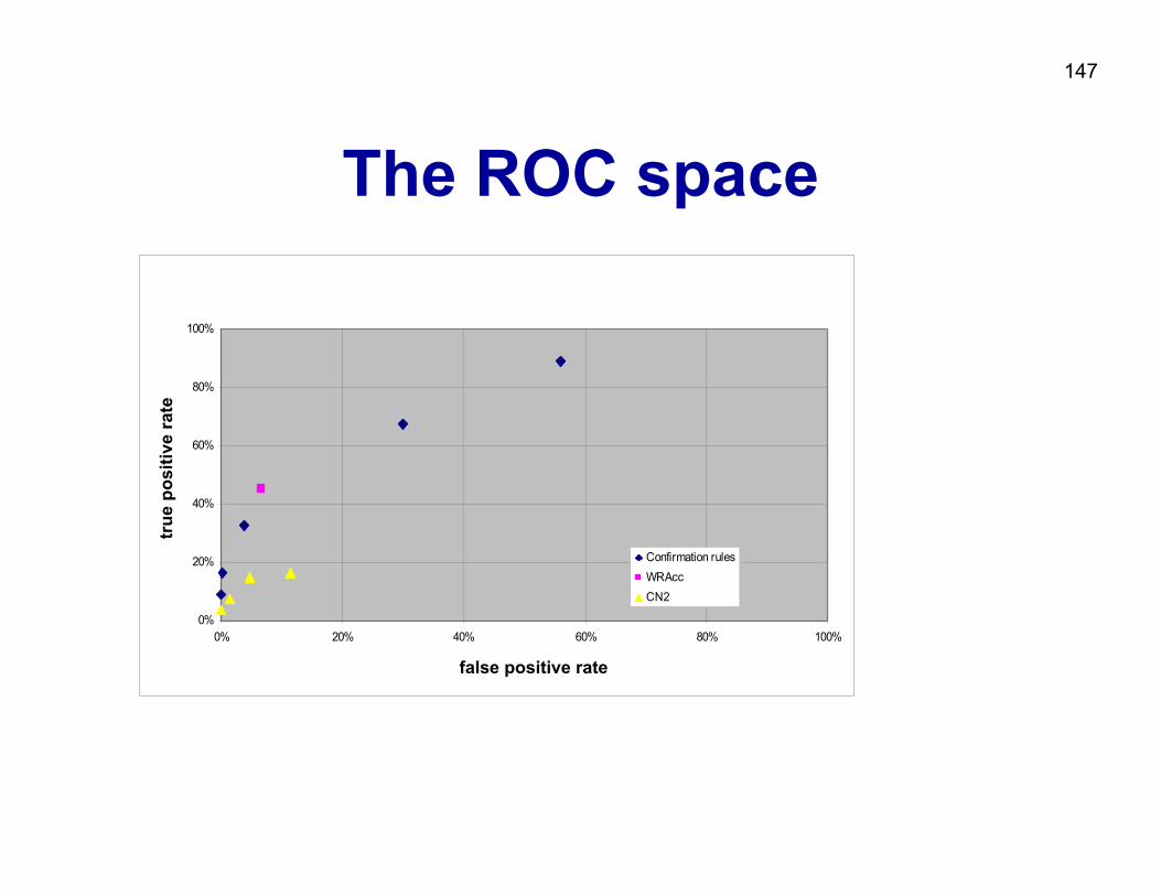
Confirmation rulesWRAccCN2
false positive rate
true
pos
itive
rate
The ROC space
148
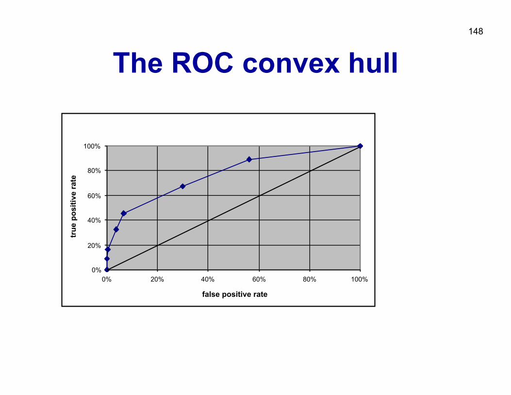
The ROC convex hull
0%
20%
40%
60%
80%
100%
0% 20% 40% 60% 80% 100%
false positive rate
true
pos
itive
rate
149
Summary of evaluation
• 10-fold cross-validation is a standard classifier evaluation method used in machine learning
• ROC analysis is very natural for rule learning and subgroup discovery– can take costs into account– here used for evaluation– also possible to use as search heuristic
150
Part III. Numeric prediction
• Baseline• Linear Regression• Regression tree• Model Tree• kNN
151
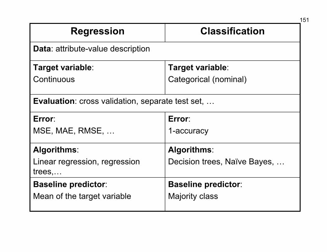
Data: attribute-value description
ClassificationRegression
Algorithms:Decision trees, Naïve Bayes, …
Algorithms:Linear regression, regression trees,…
Baseline predictor:Majority class
Baseline predictor:Mean of the target variable
Error:1-accuracy
Error:MSE, MAE, RMSE, …
Evaluation: cross validation, separate test set, …
Target variable:Categorical (nominal)
Target variable:Continuous
152
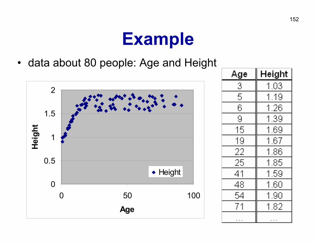
Example• data about 80 people: Age and Height
0
0.5
1
1.5
2
0 50 100
Age
Hei
ght
Height
153
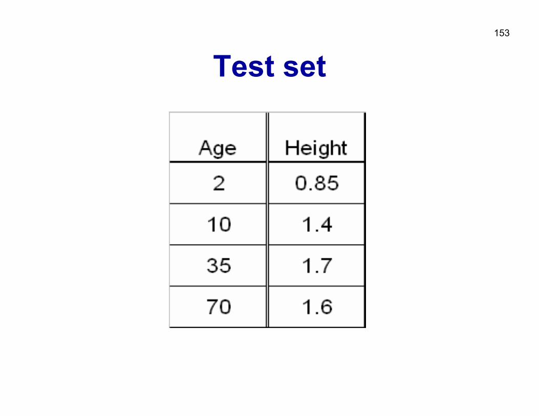
Test set
154
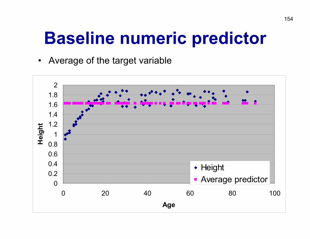
Baseline numeric predictor• Average of the target variable
00.20.40.60.8
11.21.41.61.8
2
0 20 40 60 80 100
Age
Hei
ght
HeightAverage predictor
155
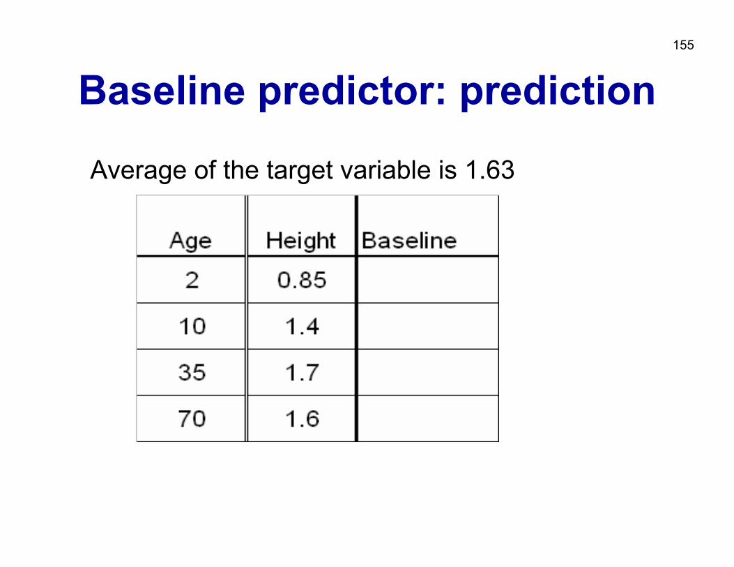
Baseline predictor: prediction
Average of the target variable is 1.63
156
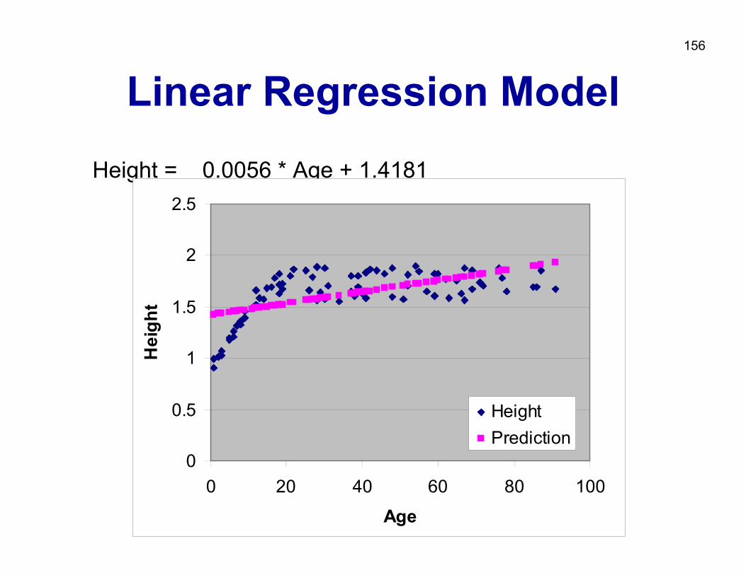
Linear Regression Model
Height = 0.0056 * Age + 1.4181
0
0.5
1
1.5
2
2.5
0 20 40 60 80 100
Age
Hei
ght
HeightPrediction
157
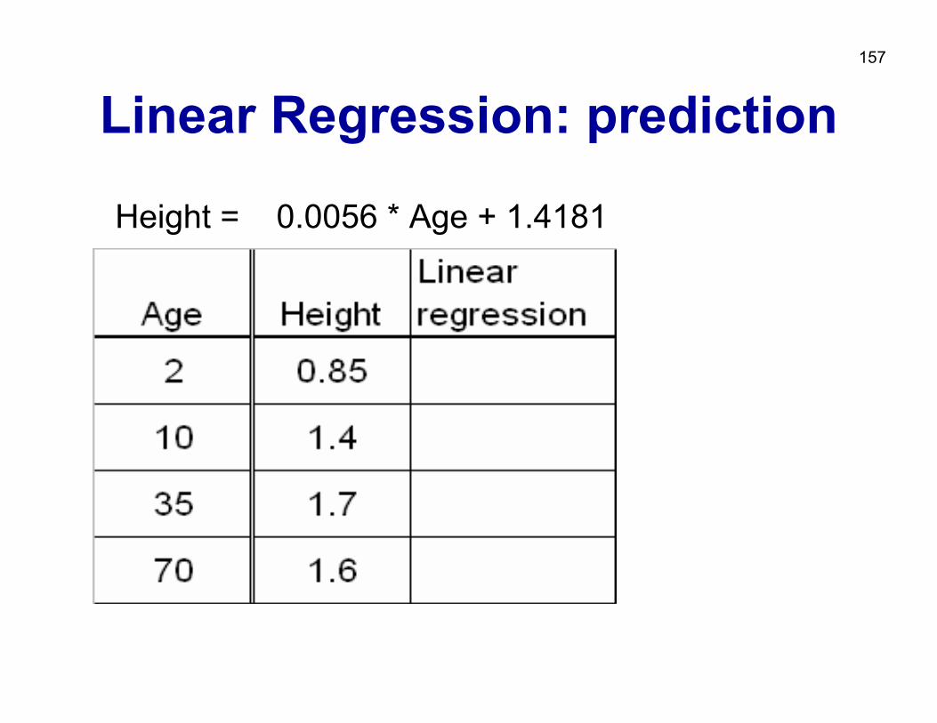
Linear Regression: prediction
Height = 0.0056 * Age + 1.4181
158
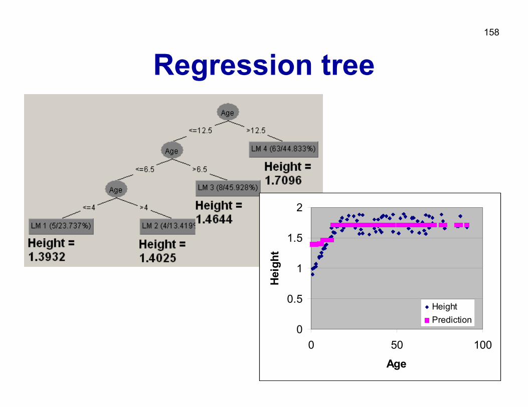
Regression tree
0
0.5
1
1.5
2
0 50 100
Age
Hei
ght
HeightPrediction
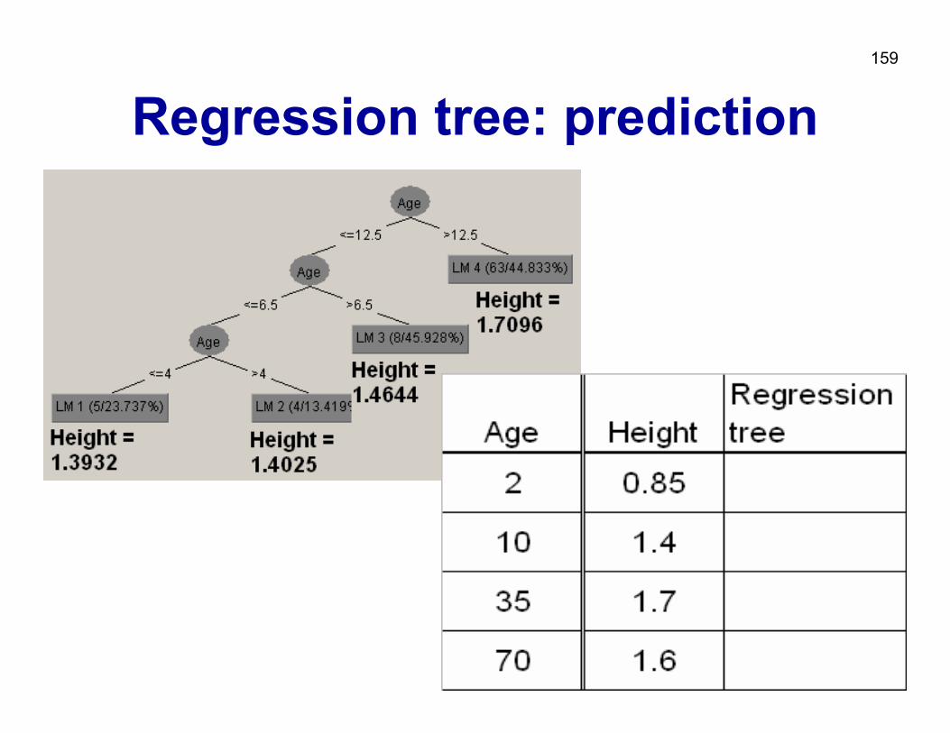
159
Regression tree: prediction
160
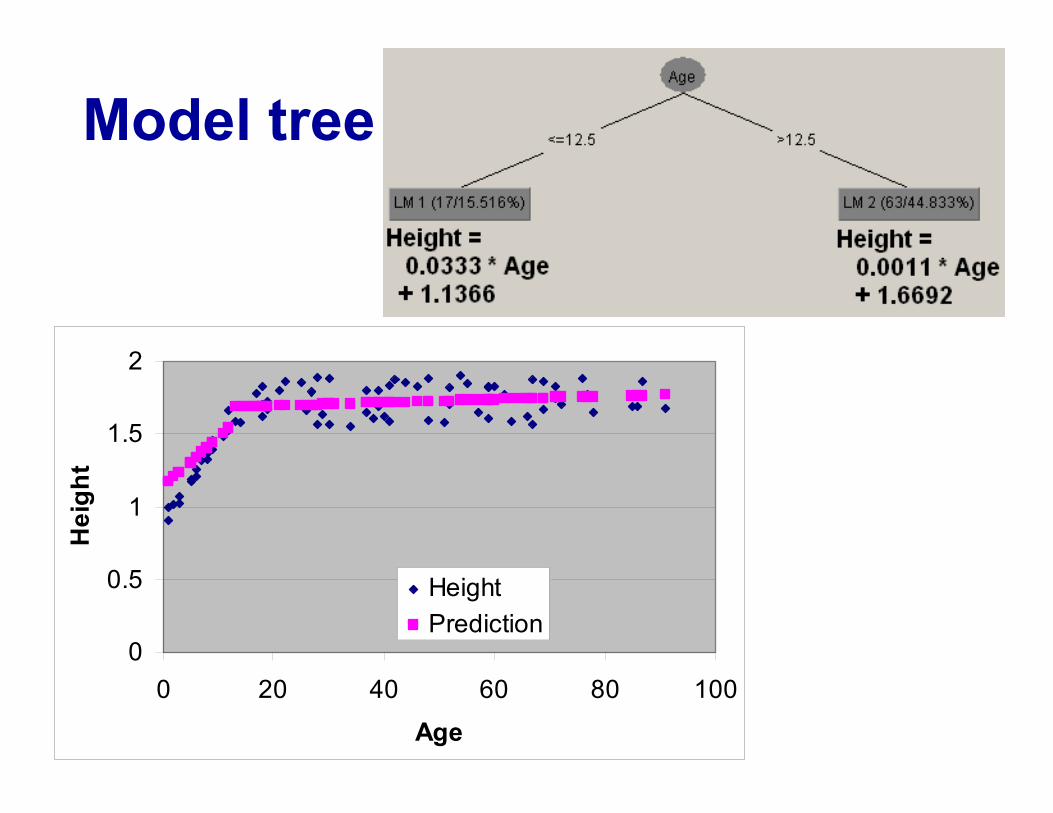
Model tree
0
0.5
1
1.5
2
0 20 40 60 80 100
Age
Hei
ght
HeightPrediction
161
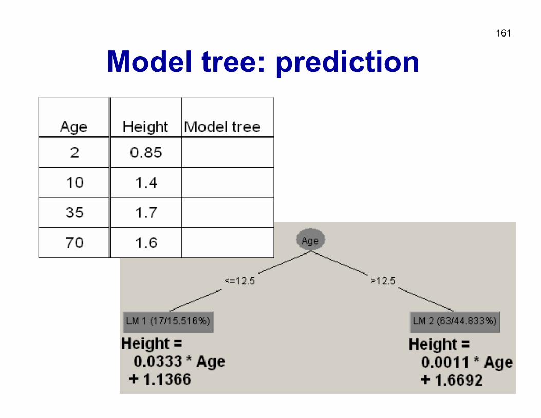
Model tree: prediction
162
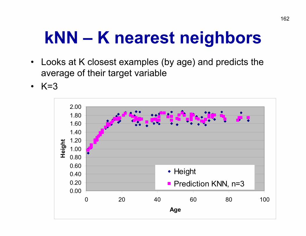
kNN – K nearest neighbors• Looks at K closest examples (by age) and predicts the
average of their target variable• K=3
0.000.200.400.600.801.001.201.401.601.802.00
0 20 40 60 80 100
Age
Hei
ght
HeightPrediction KNN, n=3
163
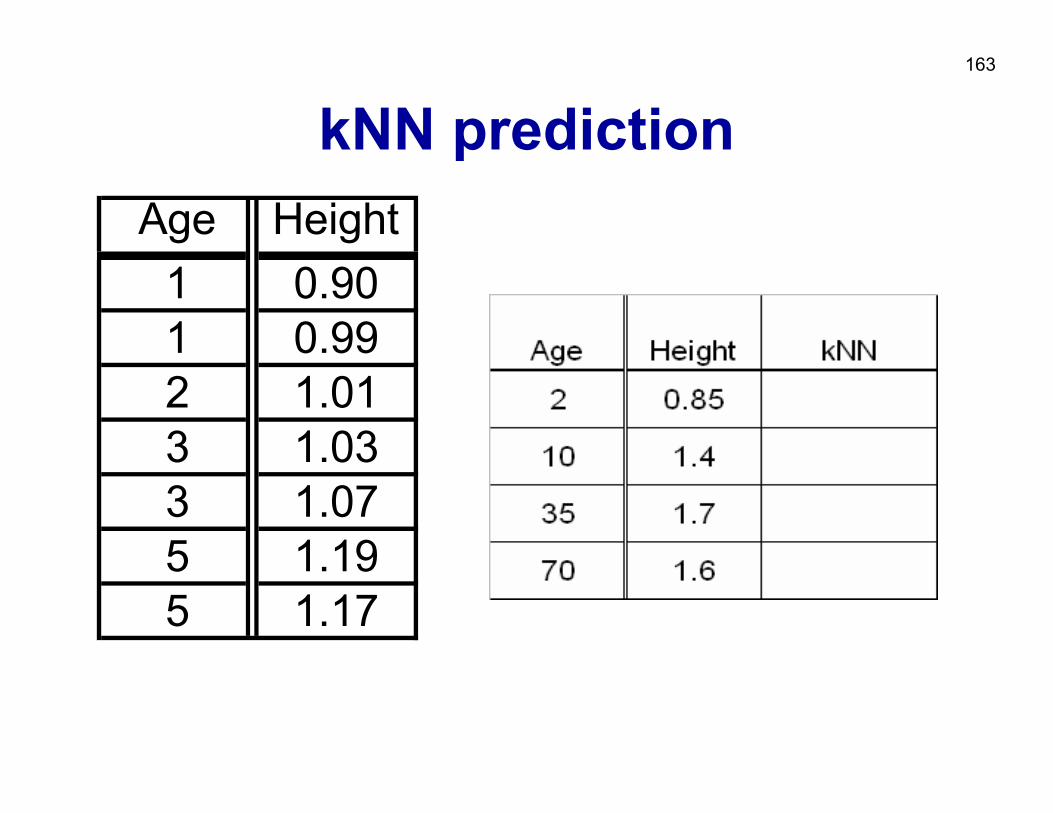
kNN predictionAge Height
1 0.901 0.992 1.013 1.033 1.075 1.195 1.17
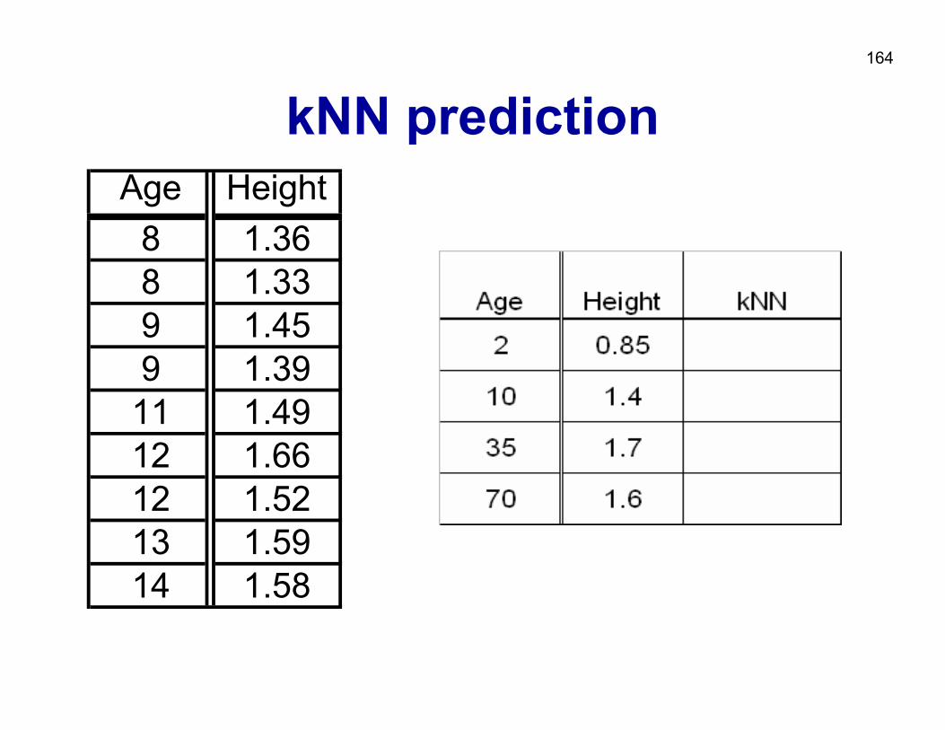
164
kNN predictionAge Height
8 1.368 1.339 1.459 1.3911 1.4912 1.6612 1.5213 1.5914 1.58
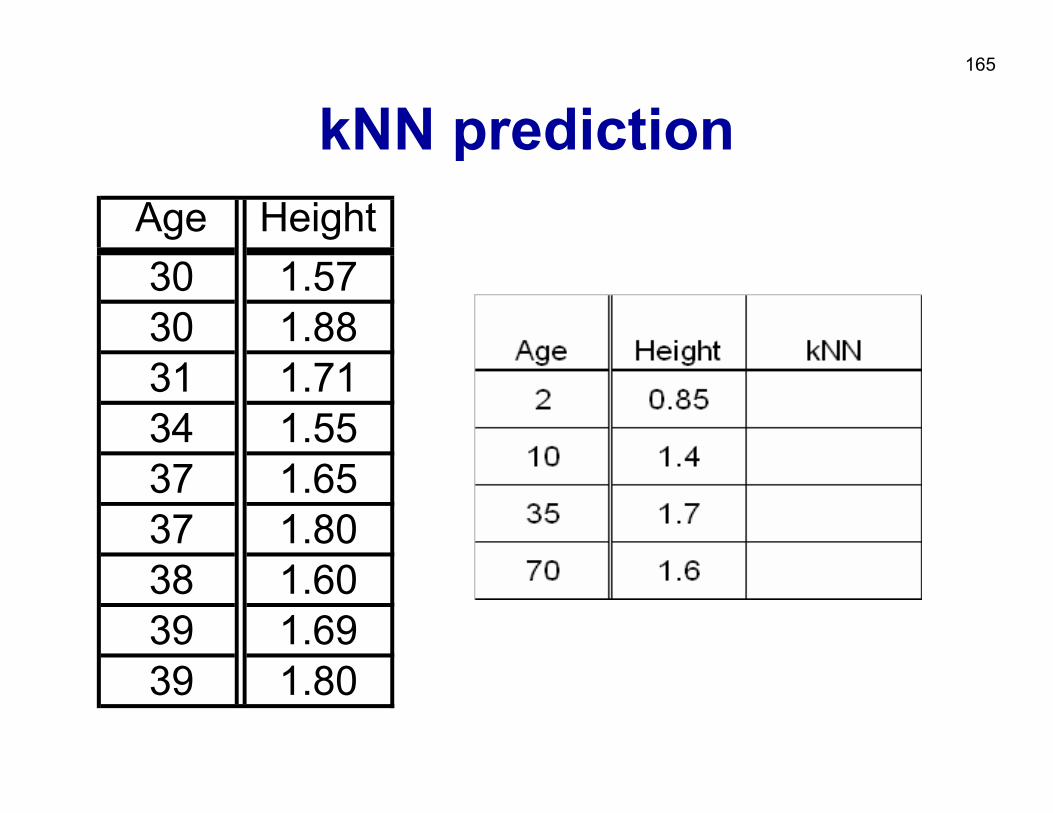
165
kNN predictionAge Height30 1.5730 1.8831 1.7134 1.5537 1.6537 1.8038 1.6039 1.6939 1.80
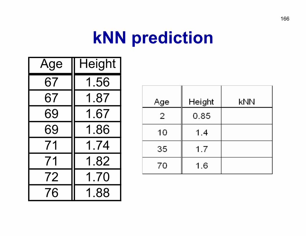
166
kNN predictionAge Height67 1.5667 1.8769 1.6769 1.8671 1.7471 1.8272 1.7076 1.88
167
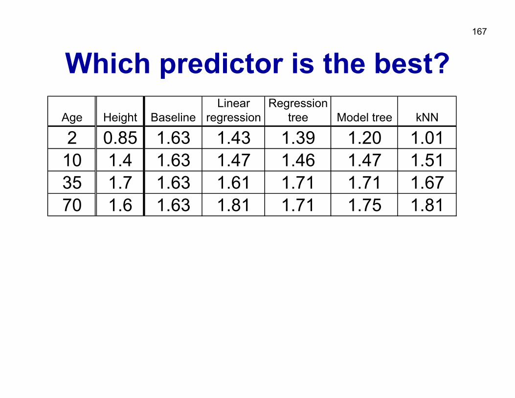
Which predictor is the best?Age Height Baseline
Linear regression
Regression tree Model tree kNN
2 0.85 1.63 1.43 1.39 1.20 1.0110 1.4 1.63 1.47 1.46 1.47 1.5135 1.7 1.63 1.61 1.71 1.71 1.6770 1.6 1.63 1.81 1.71 1.75 1.81
168
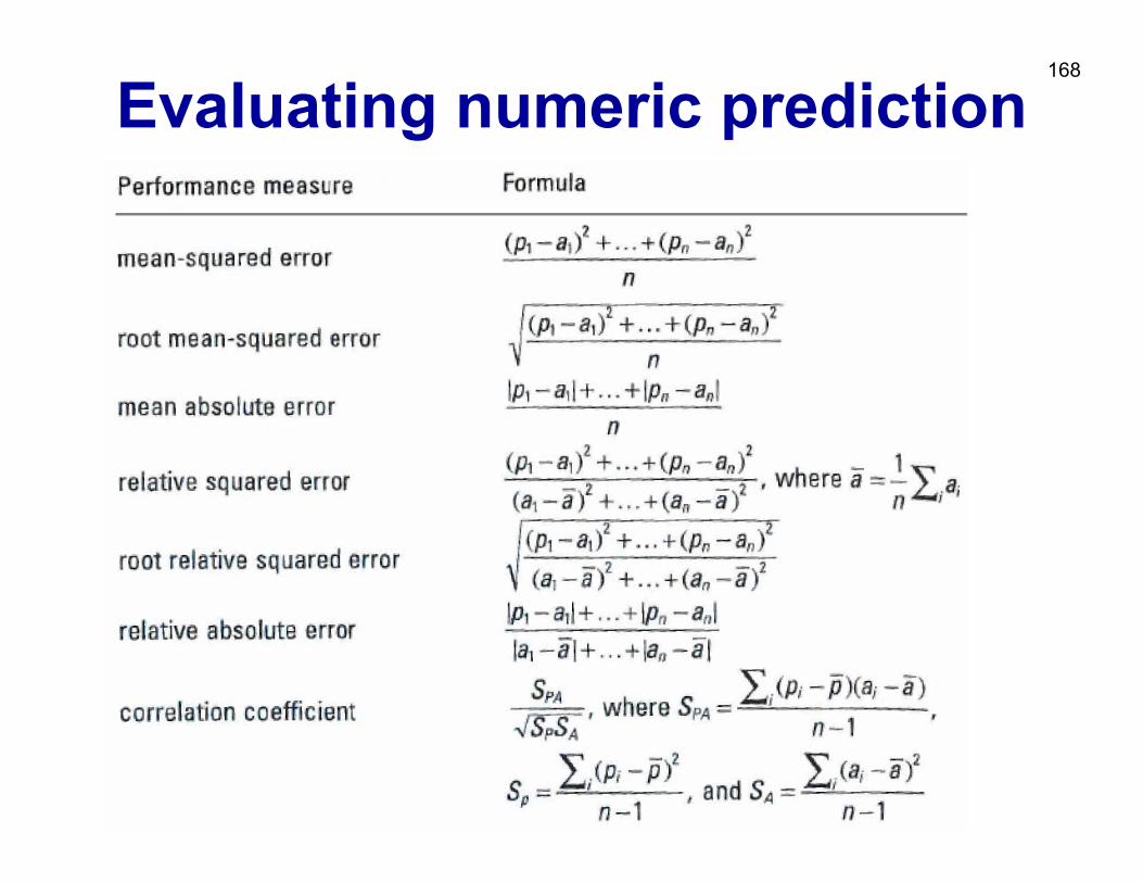
Evaluating numeric prediction
169
Part IV. Descriptive DM techniques
• Predictive vs. descriptive induction• Subgroup discovery• Association rule learning• Hierarchical clustering
170Predictive vs. descriptive induction
• Predictive induction: Inducing classifiers for solving classification and prediction tasks, – Classification rule learning, Decision tree learning, ...– Bayesian classifier, ANN, SVM, ...– Data analysis through hypothesis generation and testing
• Descriptive induction: Discovering interesting regularities in the data, uncovering patterns, ... for solving KDD tasks– Symbolic clustering, Association rule learning, Subgroup
discovery, ...– Exploratory data analysis
171
Descriptive DM
• Often used for preliminary explanatory data analysis
• User gets feel for the data and its structure• Aims at deriving descriptions of characteristics
of the data• Visualization and descriptive statistical
techniques can be used
172
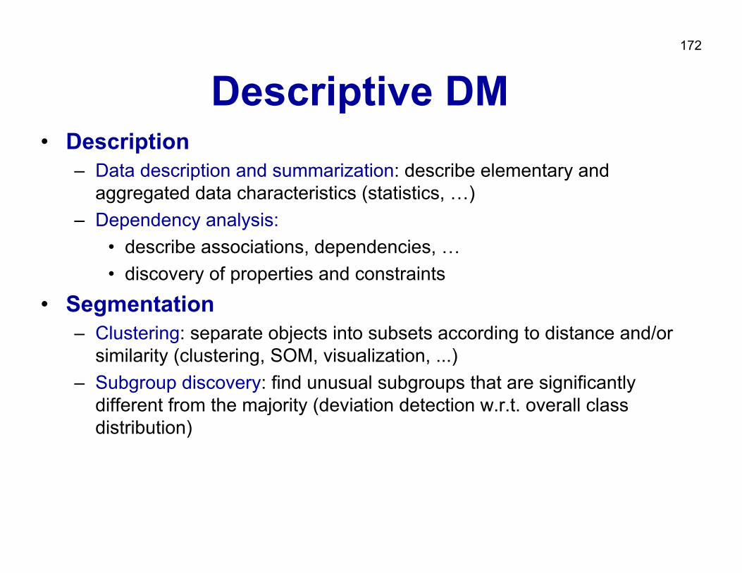
Descriptive DM• Description
– Data description and summarization: describe elementary and aggregated data characteristics (statistics, …)
– Dependency analysis:• describe associations, dependencies, …• discovery of properties and constraints
• Segmentation– Clustering: separate objects into subsets according to distance and/or
similarity (clustering, SOM, visualization, ...)– Subgroup discovery: find unusual subgroups that are significantly
different from the majority (deviation detection w.r.t. overall class distribution)
173
Predictive vs. descriptive induction: A rule learning
perspective• Predictive induction: Induces rulesets acting as
classifiers for solving classification and prediction tasks
• Descriptive induction: Discovers individual rules describing interesting regularities in the data
• Therefore: Different goals, different heuristics, different evaluation criteria
174
Supervised vs. unsupervised learning: A rule learning
perspective• Supervised learning: Rules are induced from
labeled instances (training examples with class assignment) - usually used in predictive induction
• Unsupervised learning: Rules are induced from unlabeled instances (training examples with no class assignment) - usually used in descriptive induction
• Exception: Subgroup discovery Discovers individual rules describing interesting regularities in the data from labeled examples
175
Part IV. Descriptive DM techniques
• Predictive vs. descriptive induction• Subgroup discovery• Association rule learning• Hierarchical clustering
176
Subgroup Discovery
Given: a population of individuals and a targetclass label (the property of individuals we are interested in)
Find: population subgroups that are statistically most `interesting’, e.g., are as large as possible and have most unusual statistical (distributional) characteristics w.r.t. the targetclass (property of interest)
177
Subgroup interestingnessInterestingness criteria:
– As large as possible– Class distribution as different as possible from
the distribution in the entire data set– Significant– Surprising to the user– Non-redundant– Simple– Useful - actionable
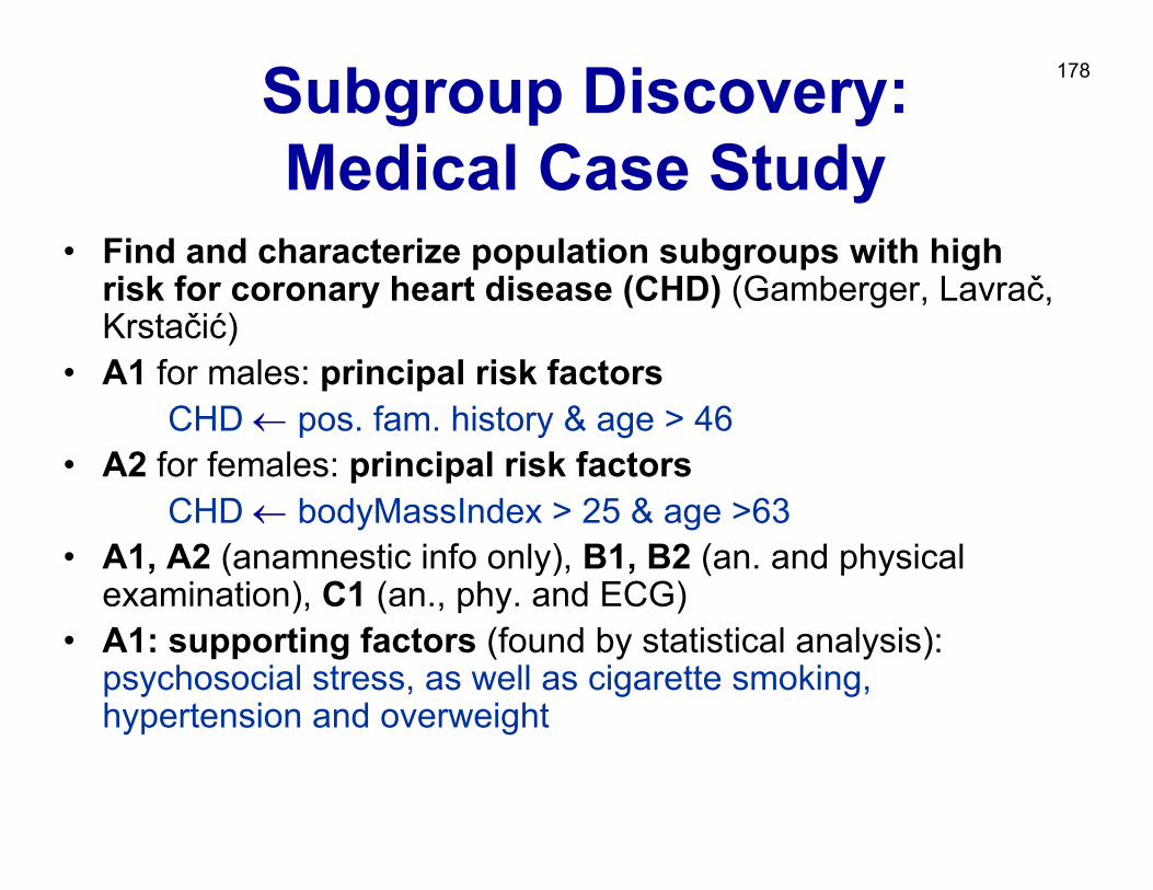
178Subgroup Discovery: Medical Case Study
• Find and characterize population subgroups with highrisk for coronary heart disease (CHD) (Gamberger, Lavrač, Krstačić)
• A1 for males: principal risk factorsCHD ← pos. fam. history & age > 46
• A2 for females: principal risk factorsCHD ← bodyMassIndex > 25 & age >63
• A1, A2 (anamnestic info only), B1, B2 (an. and physical examination), C1 (an., phy. and ECG)
• A1: supporting factors (found by statistical analysis): psychosocial stress, as well as cigarette smoking, hypertension and overweight
179
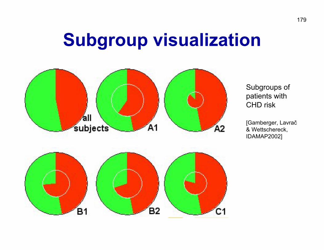
Subgroup visualization
Subgroups of patients with CHD risk
[Gamberger, Lavrač& Wettschereck, IDAMAP2002]
180
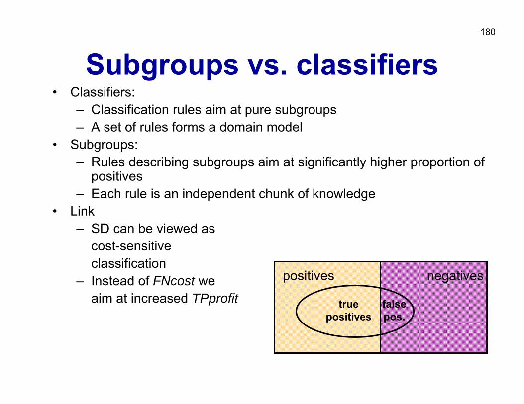
Subgroups vs. classifiers• Classifiers:
– Classification rules aim at pure subgroups– A set of rules forms a domain model
• Subgroups:– Rules describing subgroups aim at significantly higher proportion of
positives– Each rule is an independent chunk of knowledge
• Link – SD can be viewed as
cost-sensitive classification
– Instead of FNcost we aim at increased TPprofit
negativespositives
truepositives
falsepos.
181
Classification Rule Learning for Subgroup Discovery: Deficiencies• Only first few rules induced by the covering
algorithm have sufficient support (coverage)• Subsequent rules are induced from smaller and
strongly biased example subsets (pos. examples not covered by previously induced rules), which hinders their ability to detect population subgroups
• ‘Ordered’ rules are induced and interpreted sequentially as a if-then-else decision list
182
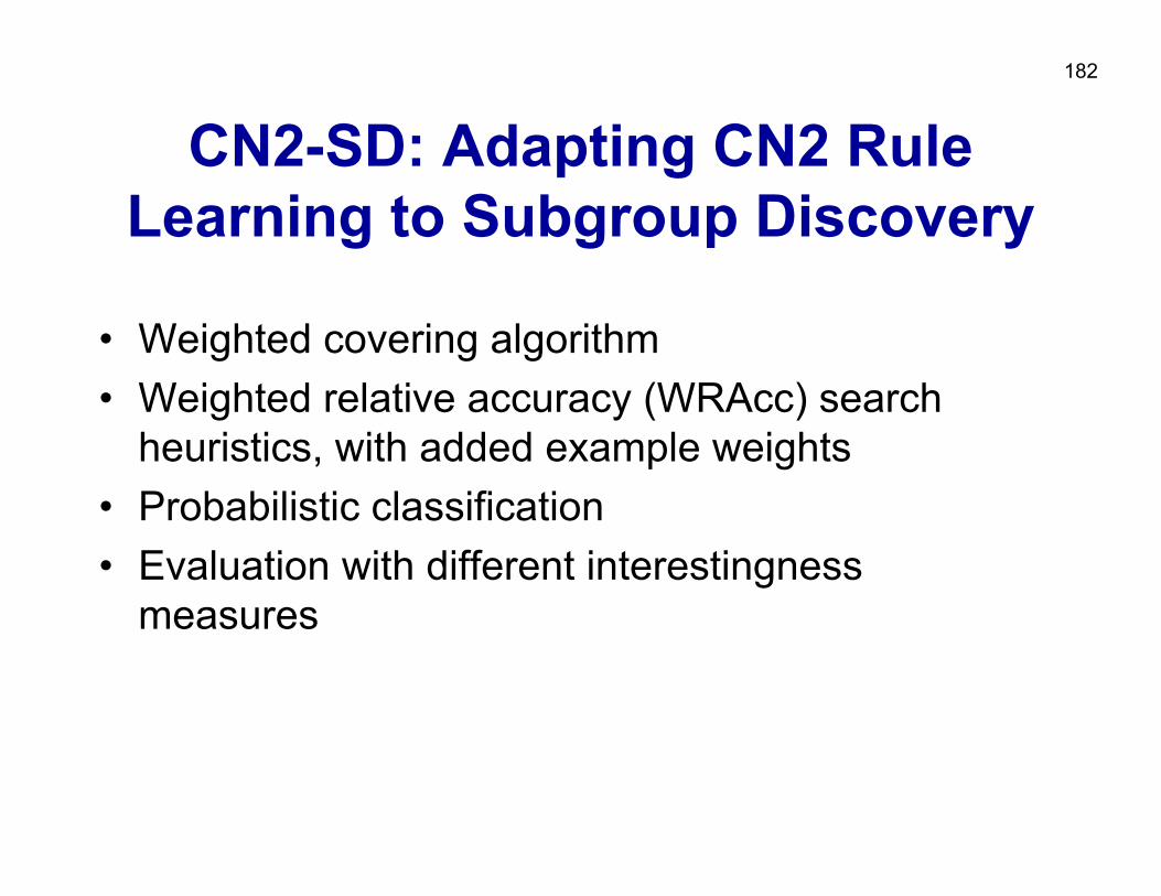
CN2-SD: Adapting CN2 Rule Learning to Subgroup Discovery
• Weighted covering algorithm• Weighted relative accuracy (WRAcc) search
heuristics, with added example weights• Probabilistic classification• Evaluation with different interestingness
measures
183
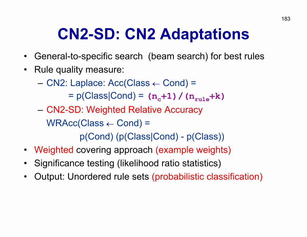
CN2-SD: CN2 Adaptations• General-to-specific search (beam search) for best rules • Rule quality measure:
– CN2: Laplace: Acc(Class ← Cond) = = p(Class|Cond) = (nc+1)/(nrule+k)
– CN2-SD: Weighted Relative AccuracyWRAcc(Class ← Cond) =
p(Cond) (p(Class|Cond) - p(Class)) • Weighted covering approach (example weights)• Significance testing (likelihood ratio statistics)• Output: Unordered rule sets (probabilistic classification)
184
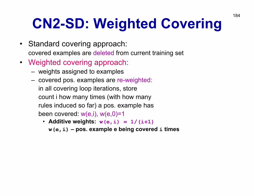
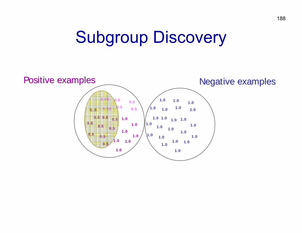
CN2-SD: Weighted Covering • Standard covering approach:
covered examples are deleted from current training set• Weighted covering approach:
– weights assigned to examples – covered pos. examples are re-weighted:
in all covering loop iterations, store count i how many times (with how many rules induced so far) a pos. example has been covered: w(e,i), w(e,0)=1
• Additive weights: w(e,i) = 1/(i+1)w(e,i) – pos. example e being covered i times
185
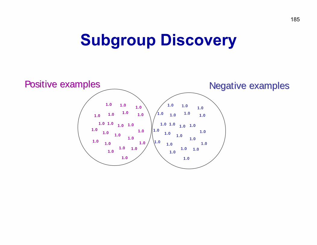
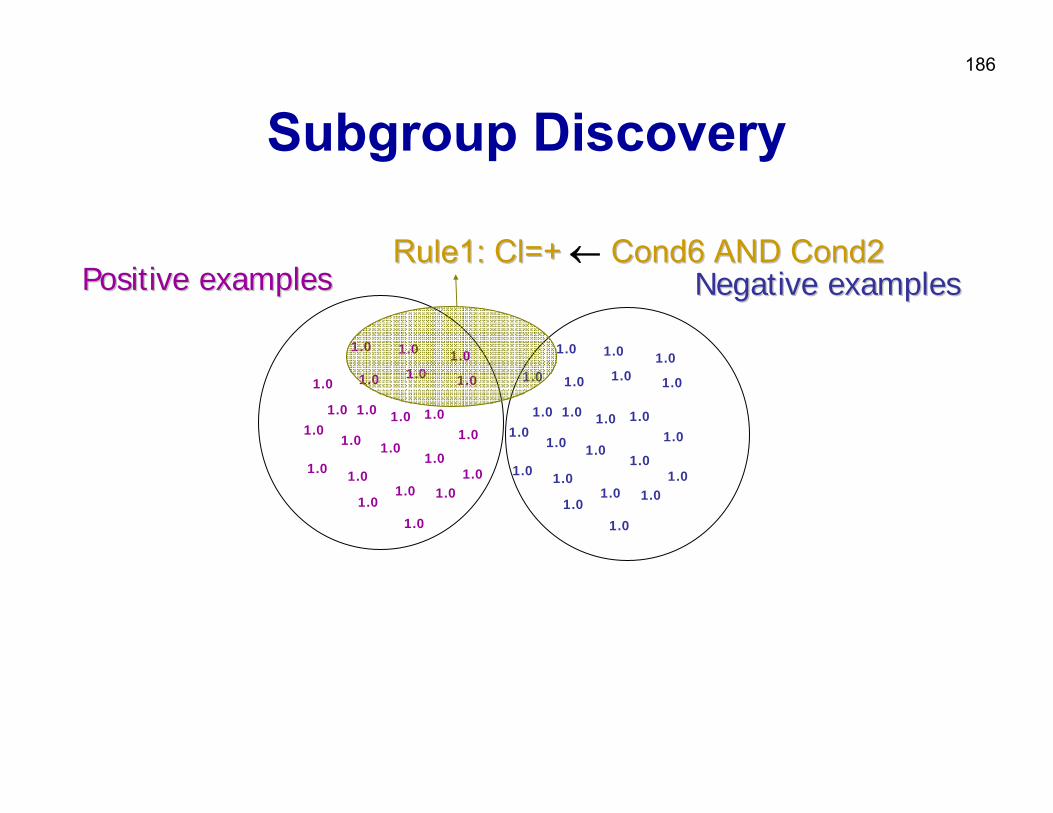
Subgroup Discovery
1.0 1.0
1.0
1.0
1.0
1.0
1.0
1.0
1.0
1.01.0 1.0
1.01.0
1.0
1.0
1.01.0
1.0
1.01.0
1.0
1.0
1.0 1.0
1.0
1.0
1.0
1.0
1.0
1.0
1.0
1.01.0
1.01.0
1.0
1.0
1.01.0
1.0
1.01.0
1.0
1.0
PositivePositive examplesexamples NNegativeegative examplesexamples
1.0
186
Subgroup Discovery
1.0 1.0
1.0
1.0
1.0
1.0
1.0
1.0
1.0
1.01.0 1.0
1.01.0
1.0
1.0
1.01.0
1.0
1.01.0
1.0
1.0
1.0 1.0
1.0
1.0
1.0
1.0
1.0
1.0
1.0
1.01.0 1.0
1.01.0
1.0
1.0
1.01.0
1.0
1.01.0
1.0
1.0
PositivePositive examplesexamples NNegativeegative examplesexamplesRule1: Rule1: ClCl=+ =+ ← Cond6 AND Cond2Cond6 AND Cond2
187
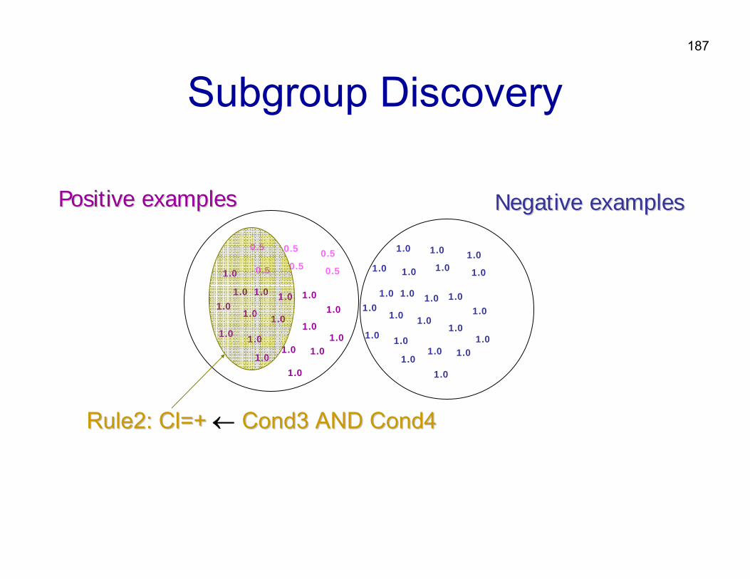
Subgroup Discovery
0.5 0.5
1.0
0.5
0.5
1.0
1.0
1.0
1.0
0.51.0 0.5
1.01.0
1.0
1.0
1.01.0
1.0
1.01.0
1.0
1.0
1.0 1.0
1.0
1.0
1.0
1.0
1.0
1.0
1.0
1.01.0 1.0
1.01.0
1.0
1.0
1.01.0
1.0
1.01.0
1.0
1.0
PositivePositive examplesexamples NNegativeegative examplesexamples
Rule2: Rule2: ClCl=+ =+ ← Cond3 AND Cond4Cond3 AND Cond4
188
Subgroup Discovery
0.5 0.5
0.5
0.25
0.5
0.5
0.5
0.5
1.0
0.50..5 0.25
0.51.0
1.0
0.5
0.50.5
1.0
1.01.0
0.5
1.0
1.0 1.0
1.0
1.0
1.0
1.0
1.0
1.0
1.0
1.01.0 1.0
1.01.0
1.0
1.0
1.01.0
1.0
1.01.0
1.0
1.0
PositivePositive examplesexamples NNegativeegative examplesexamples
189
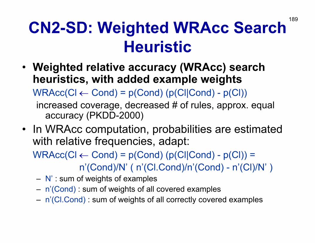
CN2-SD: Weighted WRAcc Search Heuristic
• Weighted relative accuracy (WRAcc) search heuristics, with added example weights WRAcc(Cl ← Cond) = p(Cond) (p(Cl|Cond) - p(Cl))increased coverage, decreased # of rules, approx. equal
accuracy (PKDD-2000)• In WRAcc computation, probabilities are estimated
with relative frequencies, adapt:WRAcc(Cl ← Cond) = p(Cond) (p(Cl|Cond) - p(Cl)) =
n’(Cond)/N’ ( n’(Cl.Cond)/n’(Cond) - n’(Cl)/N’ )– N’ : sum of weights of examples– n’(Cond) : sum of weights of all covered examples– n’(Cl.Cond) : sum of weights of all correctly covered examples
190
Part IV. Descriptive DM techniques
• Predictive vs. descriptive induction• Subgroup discovery• Association rule learning• Hierarchical clustering
191
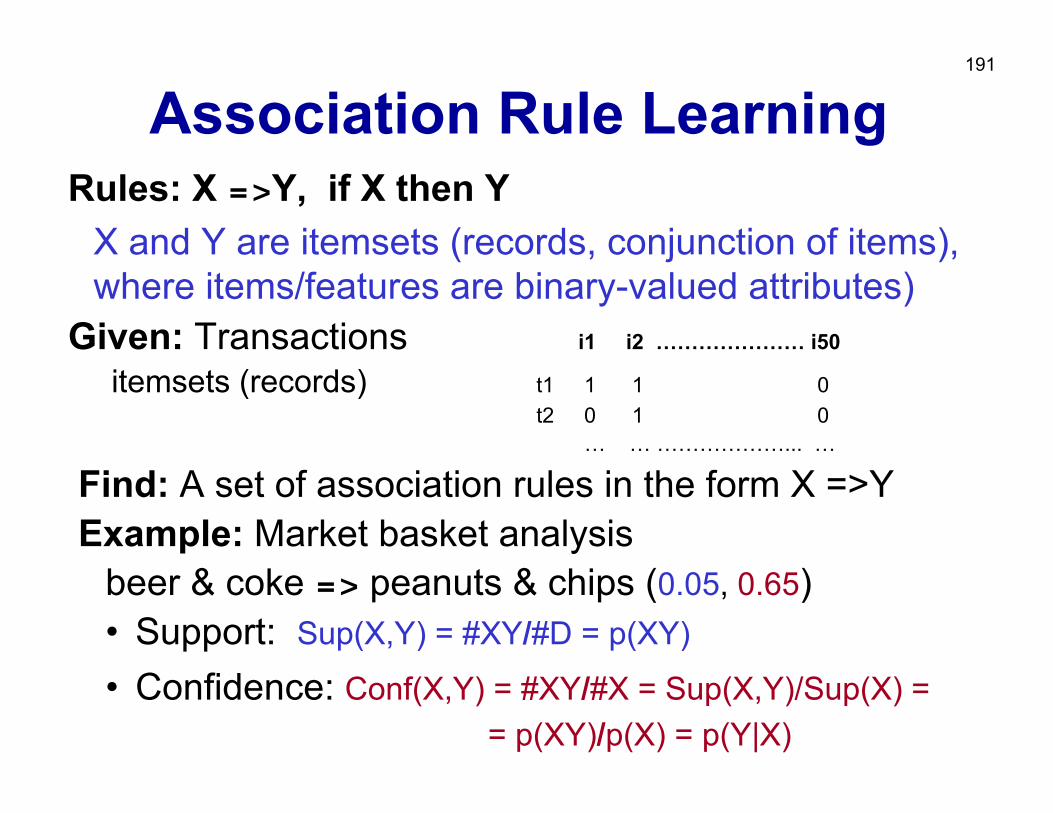
Association Rule LearningRules: X =>Y, if X then Y
X and Y are itemsets (records, conjunction of items), where items/features are binary-valued attributes)
Given: Transactions i1 i2 ………………… i50
itemsets (records) t1 1 1 0 t2 0 1 0
… … ………………... …
Find: A set of association rules in the form X =>YExample: Market basket analysis
beer & coke => peanuts & chips (0.05, 0.65)• Support: Sup(X,Y) = #XY/#D = p(XY)
• Confidence: Conf(X,Y) = #XY/#X = Sup(X,Y)/Sup(X) == p(XY)/p(X) = p(Y|X)
192
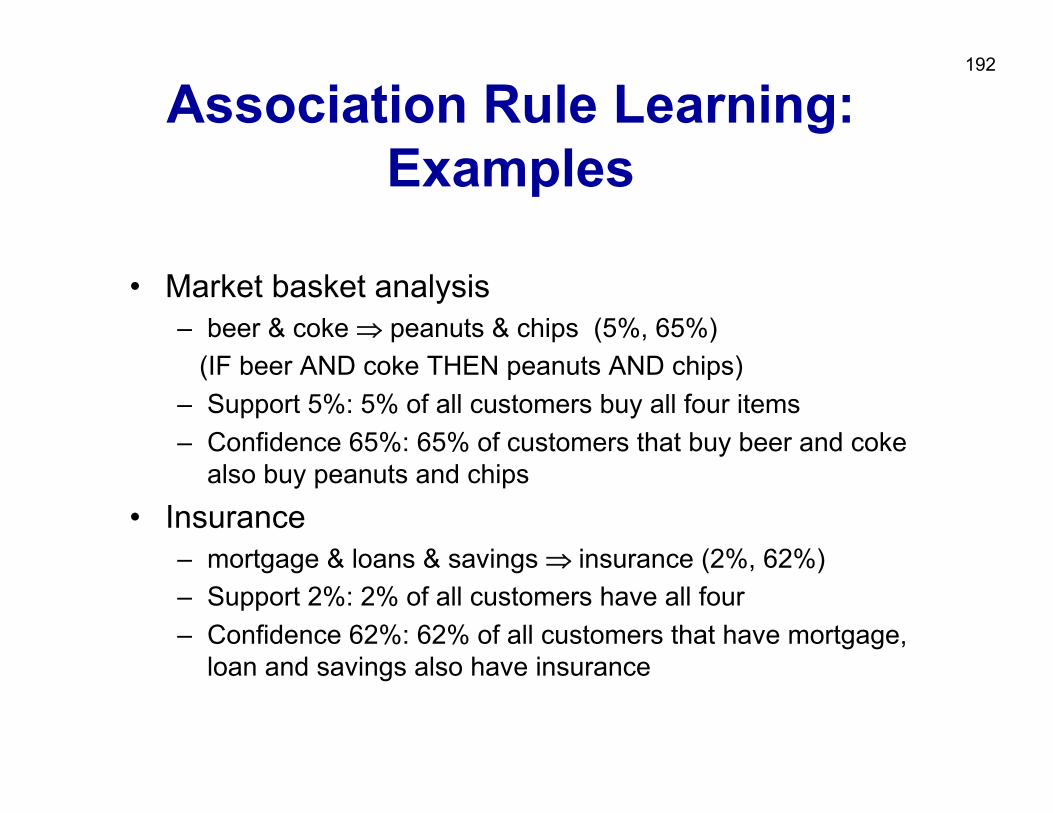
Association Rule Learning: Examples
• Market basket analysis– beer & coke ⇒ peanuts & chips (5%, 65%)
(IF beer AND coke THEN peanuts AND chips)– Support 5%: 5% of all customers buy all four items– Confidence 65%: 65% of customers that buy beer and coke
also buy peanuts and chips
• Insurance– mortgage & loans & savings ⇒ insurance (2%, 62%)– Support 2%: 2% of all customers have all four – Confidence 62%: 62% of all customers that have mortgage,
loan and savings also have insurance
193
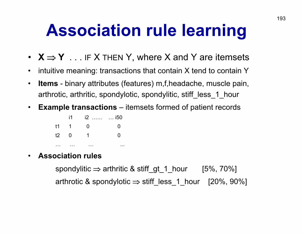
Association rule learning• X ⇒ Y . . . IF X THEN Y, where X and Y are itemsets• intuitive meaning: transactions that contain X tend to contain Y
• Items - binary attributes (features) m,f,headache, muscle pain, arthrotic, arthritic, spondylotic, spondylitic, stiff_less_1_hour
• Example transactions – itemsets formed of patient recordsi1 i2 …… … i50
t1 1 0 0
t2 0 1 0
… … … ...
• Association rulesspondylitic ⇒ arthritic & stiff_gt_1_hour [5%, 70%]
arthrotic & spondylotic ⇒ stiff_less_1_hour [20%, 90%]
194
Association Rule LearningGiven: a set of transactions D
Find: all association rules that hold on the set of transactions that have – user defined minimum support, i.e., support > MinSup, and
– user defined minimum confidence, i.e., confidence > MinConf
It is a form of exploratory data analysis, rather than hypothesis verification
195
Searching for the associations
• Find all large itemsets
• Use the large itemsets to generate association rules
• If XY is a large itemset, compute
r =support(XY) / support(X)
• If r > MinConf, then X ⇒ Y holds (support > MinSup, as XY is large)
196
Large itemsets
• Large itemsets are itemsets that appear in at least MinSup transaction
• All subsets of a large itemset are large itemsets (e.g., if A,B appears in at least MinSup transactions, so do A and B)
• This observation is the basis for very efficient algorithms for association rules discovery (linear in the number of transactions)
197
Association vs. Classificationrules rules
• Exploration of dependencies
• Different combinations of dependent and independent attributes
• Complete search (all rules found)
• Focused prediction• Predict one attribute
(class) from the others• Heuristic search (subset
of rules found)
198
Part IV. Descriptive DM techniques
• Predictive vs. descriptive induction• Subgroup discovery• Association rule learning• Hierarchical clustering
199
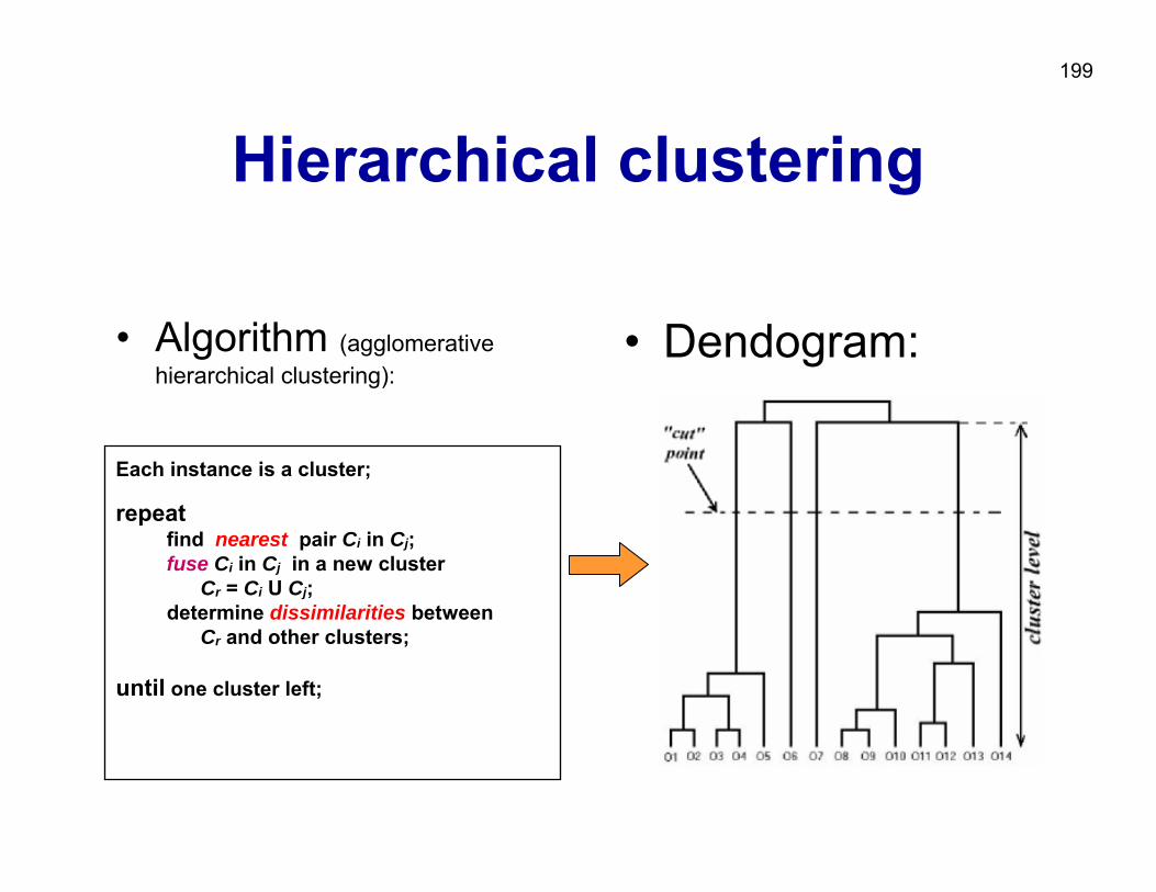
Hierarchical clustering
• Algorithm (agglomerative hierarchical clustering):
Each instance is a cluster;
repeatfind nearest pair Ci in Cj;fuse Ci in Cj in a new cluster
Cr = Ci U Cj;determine dissimilarities between
Cr and other clusters;
until one cluster left;
• Dendogram:
200
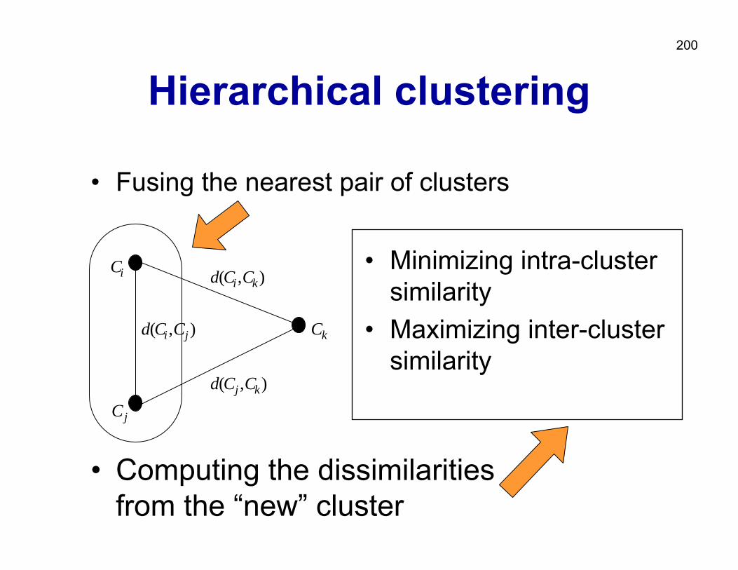
Hierarchical clustering
• Fusing the nearest pair of clusters
iC
jC
kC),( ji CCd
),( ki CCd
),( kj CCd
• Minimizing intra-cluster similarity
• Maximizing inter-cluster similarity
• Computing the dissimilarities from the “new” cluster
201
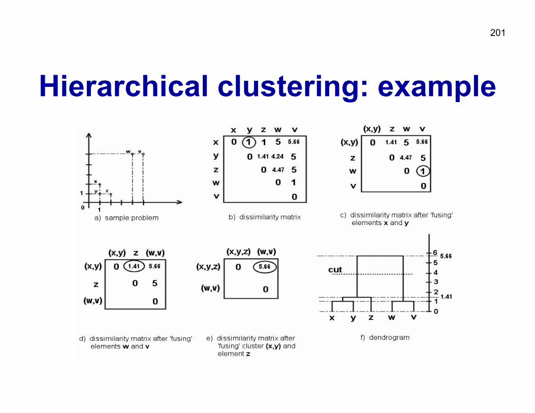
Hierarchical clustering: example
202
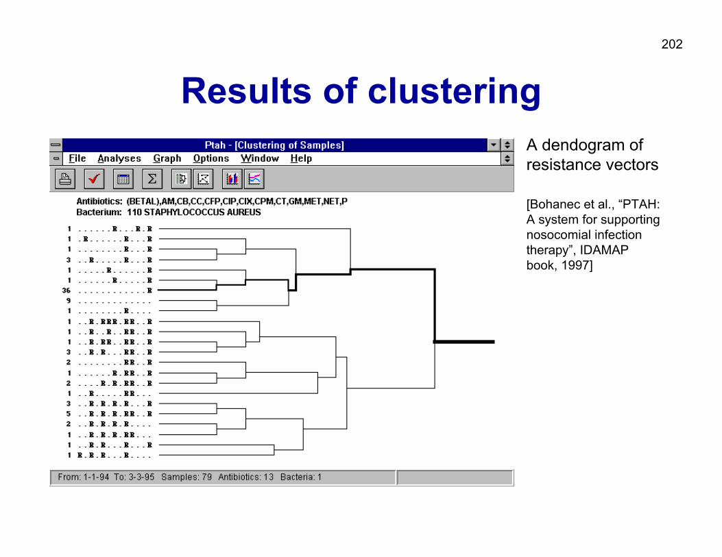
Results of clusteringA dendogram of resistance vectors
[Bohanec et al., “PTAH: A system for supporting nosocomial infection therapy”, IDAMAP book, 1997]
203Part V: Relational Data Mining
• Learning as search• What is RDM?• Propositionalization techniques• Inductive Logic Programming

204
Learning as search • Structuring the state space: Representing a partial
order of hypotheses (e.g. rules) as a graph– nodes: concept descriptions (hypotheses/rules)– arcs defined by specialization/generalization
operators : an arc from parent to child exists if-and-only-if parent is a proper most specific generalization of child
• Specialization operators: e.g., adding conditions: s(A=a2 & B=b1) = {A=a2 & B=b1 & D=d1, A=a2 & B=b1 & D=d2}
• Generalization operators: e.g., dropping conditions: g(A=a2 & B=b1) = {A=a2, B=b1}
• Partial order of hypotheses defines a lattice (called a refinement graph)
205
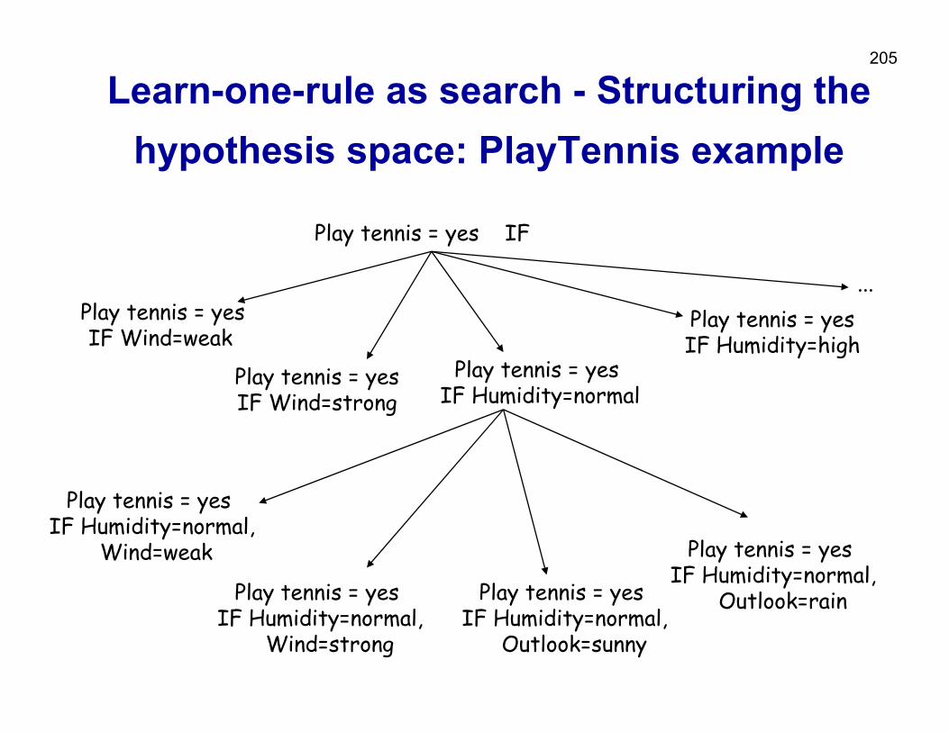
Learn-one-rule as search - Structuring the hypothesis space: PlayTennis example
Play tennis = yes IF
Play tennis = yes IF Wind=weak
Play tennis = yesIF Wind=strong
Play tennis = yes IF Humidity=normal
Play tennis = yesIF Humidity=high
Play tennis = yes IF Humidity=normal,
Wind=weak
Play tennis = yes IF Humidity=normal,
Wind=strong
Play tennis = yes IF Humidity=normal,
Outlook=sunny
Play tennis = yes IF Humidity=normal,
Outlook=rain
...
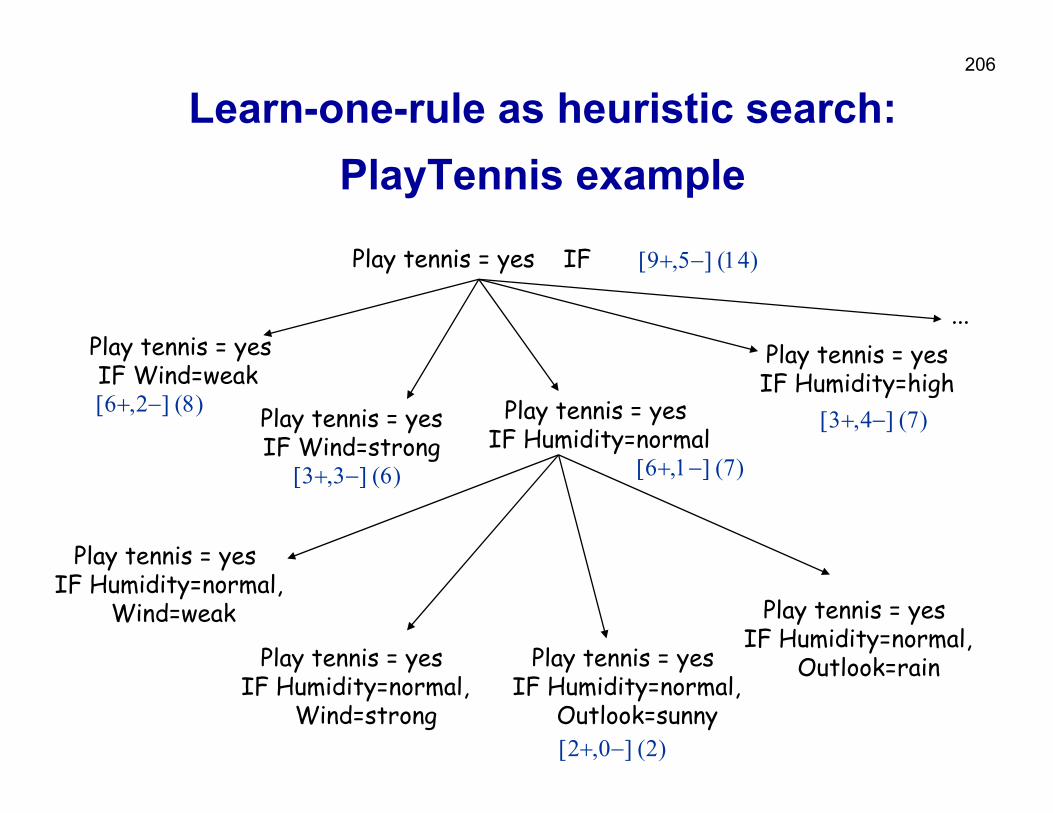
206
Learn-one-rule as heuristic search: PlayTennis example
Play tennis = yes IF
Play tennis = yes IF Wind=weak
Play tennis = yesIF Wind=strong
Play tennis = yes IF Humidity=normal
Play tennis = yesIF Humidity=high
Play tennis = yes IF Humidity=normal,
Wind=weak
Play tennis = yes IF Humidity=normal,
Wind=strong
Play tennis = yes IF Humidity=normal,
Outlook=sunny
Play tennis = yes IF Humidity=normal,
Outlook=rain
[9+,5−] (14)
[6+,2−] (8)
[3+,3−] (6) [6+,1−] (7)
[3+,4−] (7)
...
[2+,0−] (2)
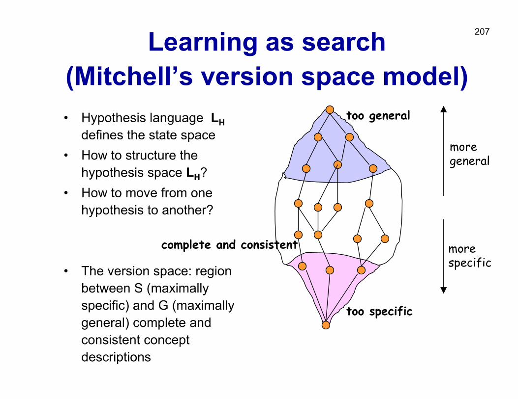
207Learning as search (Mitchell’s version space model)• Hypothesis language LH
defines the state space • How to structure the
hypothesis space LH?• How to move from one
hypothesis to another?
• The version space: region between S (maximally specific) and G (maximally general) complete and consistent concept descriptions
too general
too specific
moregeneral
morespecific
complete and consistent
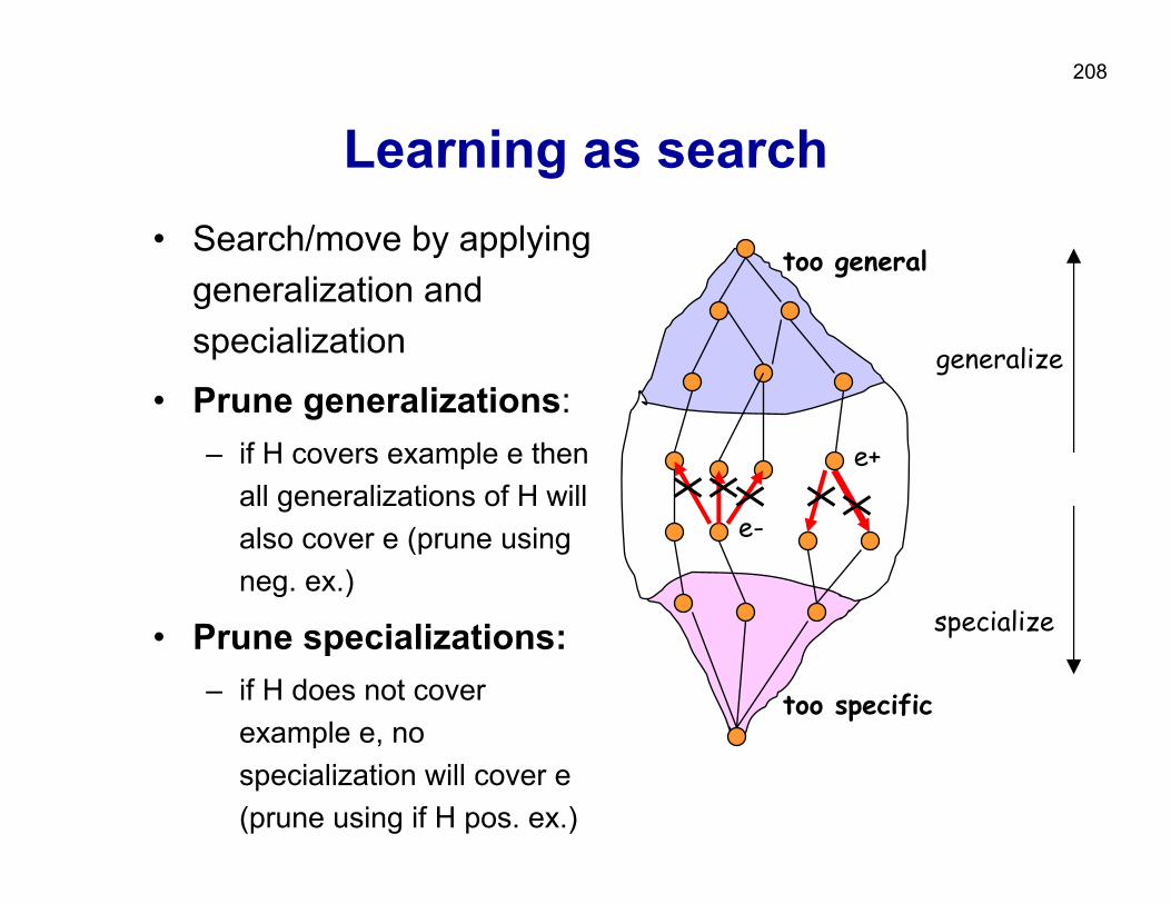
208
Learning as search• Search/move by applying
generalization and specialization
• Prune generalizations: – if H covers example e then
all generalizations of H will also cover e (prune using neg. ex.)
• Prune specializations:– if H does not cover
example e, no specialization will cover e (prune using if H pos. ex.)
too general
too specific
generalize
specialize
e-
e+
209
Learning as search: Learner’s ingredients
– structure of the search space (specialization and generalization operators)
– search strategy• depth-first• breath-first• heuristic search (best first, hill-climbing, beam search)
– search heuristics • measure of attribute ‘informativity’• measure of ‘expected classification accuracy’ (relative
frequency, Laplace estimate, m-estimate), ...
– stopping criteria (consistency, completeness, statistical significance, …)
210Learn-one-rule:search heuristics
• Assume a two-class problem• Two classes (+,-), learn rules for + class (Cl). • Search for specializations R’ of a rule R = Cl ← Cond
from the RuleBase.• Specializarion R’ of rule R = Cl ← Cond
has the form R’ = Cl ← Cond & Cond’• Heuristic search for rules: find the ‘best’ Cond’ to be
added to the current rule R, such that rule accuracy is improved, e.g., such that Acc(R’) > Acc(R)– where the expected classification accuracy can be
estimated as A(R) = p(Cl|Cond)
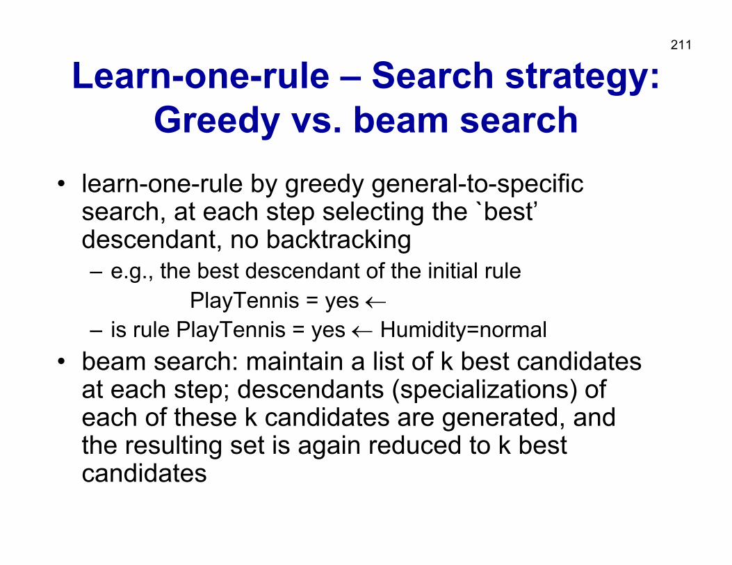
211
Learn-one-rule – Search strategy: Greedy vs. beam search
• learn-one-rule by greedy general-to-specific search, at each step selecting the `best’descendant, no backtracking– e.g., the best descendant of the initial rule
PlayTennis = yes ←– is rule PlayTennis = yes ← Humidity=normal
• beam search: maintain a list of k best candidates at each step; descendants (specializations) of each of these k candidates are generated, and the resulting set is again reduced to k best candidates
212Part V: Relational Data Mining
• Learning as search• What is RDM?• Propositionalization techniques• Inductive Logic Programming
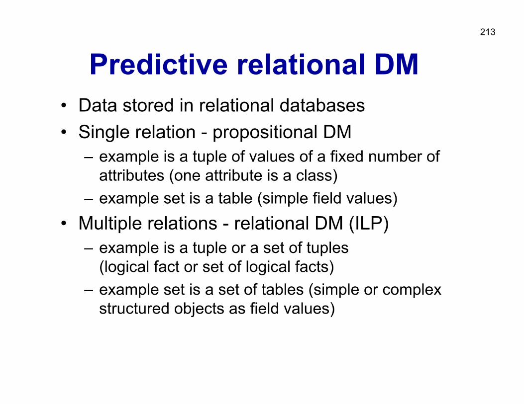
213
Predictive relational DM• Data stored in relational databases• Single relation - propositional DM
– example is a tuple of values of a fixed number of attributes (one attribute is a class)
– example set is a table (simple field values)• Multiple relations - relational DM (ILP)
– example is a tuple or a set of tuples(logical fact or set of logical facts)
– example set is a set of tables (simple or complex structured objects as field values)
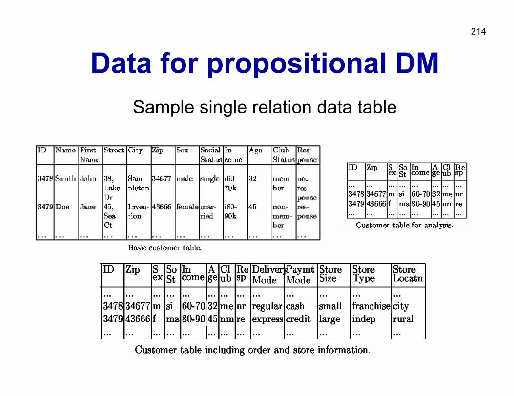
214
Data for propositional DMSample single relation data table
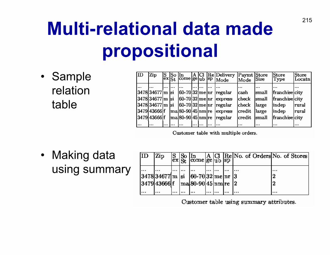
215Multi-relational data made propositional
• Sample multi-relation data table
• Making data propositional: using summary attributes
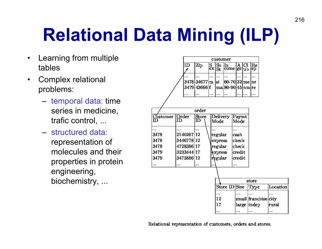
216
Relational Data Mining (ILP)• Learning from multiple
tables• Complex relational
problems:– temporal data: time
series in medicine, trafic control, ...
– structured data:representation of molecules and their properties in protein engineering, biochemistry, ...
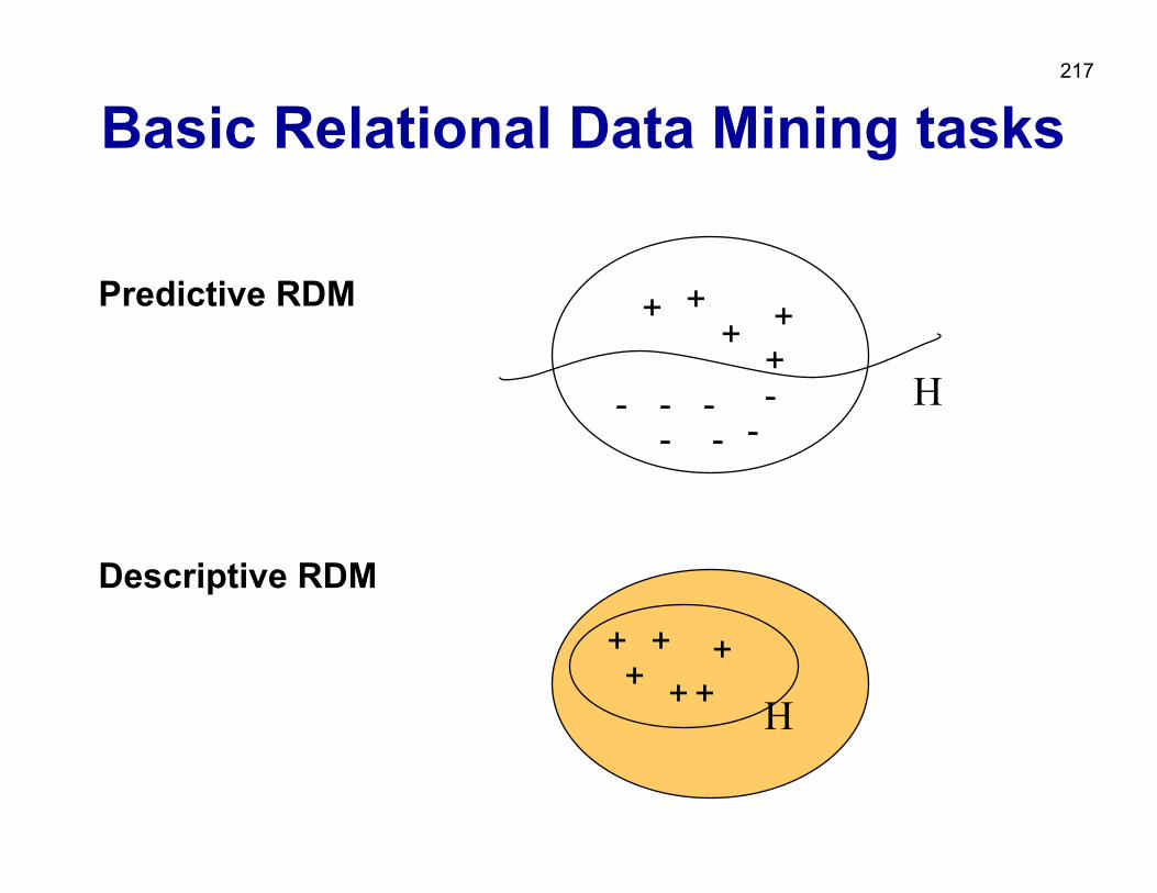
217
Basic Relational Data Mining tasks
Predictive RDM
Descriptive RDM
+
-
++ +
+- -
---
-
+ + ++++
Η
Η
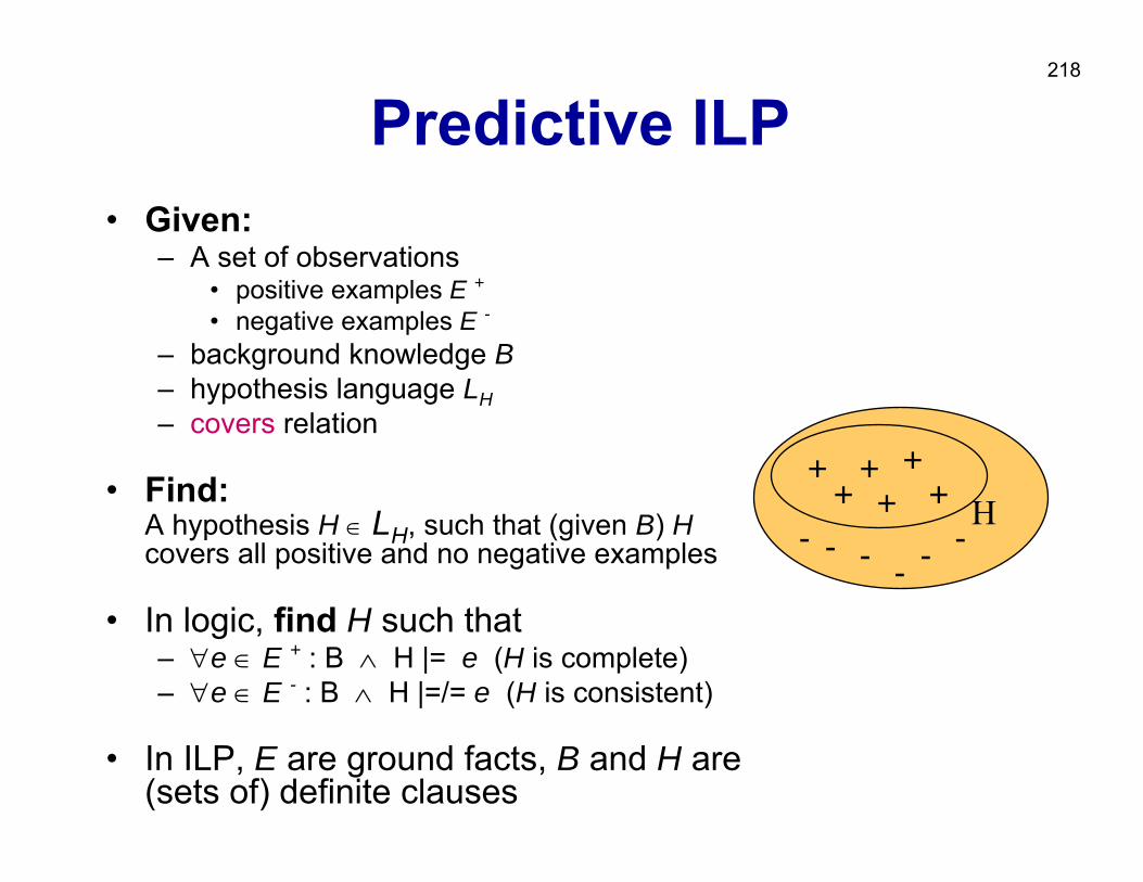
218
Predictive ILP• Given:
– A set of observations• positive examples E +• negative examples E -
– background knowledge B– hypothesis language LH– covers relation
• Find:A hypothesis H ∈ LH, such that (given B) Hcovers all positive and no negative examples
• In logic, find H such that– ∀e ∈ E + : B ∧ H |= e (H is complete)– ∀e ∈ E - : B ∧ H |=/= e (H is consistent)
• In ILP, E are ground facts, B and H are (sets of) definite clauses
+ + ++++
- - - ---
Η
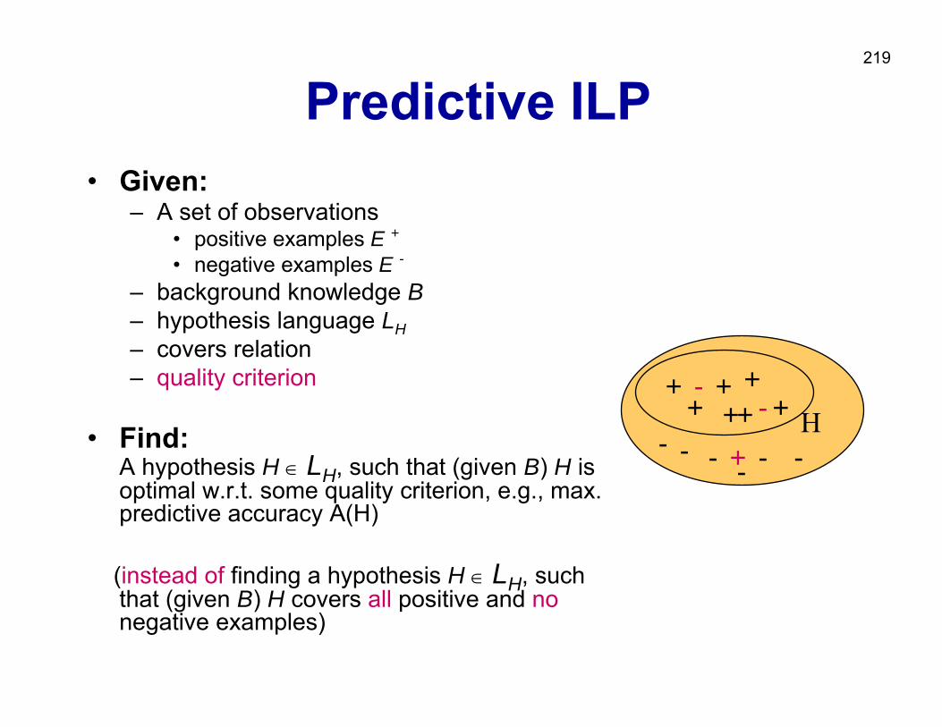
219
Predictive ILP• Given:
– A set of observations• positive examples E +• negative examples E -
– background knowledge B– hypothesis language LH– covers relation– quality criterion
• Find:A hypothesis H ∈ LH, such that (given B) H is optimal w.r.t. some quality criterion, e.g., max. predictive accuracy A(H)
(instead of finding a hypothesis H ∈ LH, such that (given B) H covers all positive and nonegative examples)
+ +++
- - - ---
Η+
+++
--
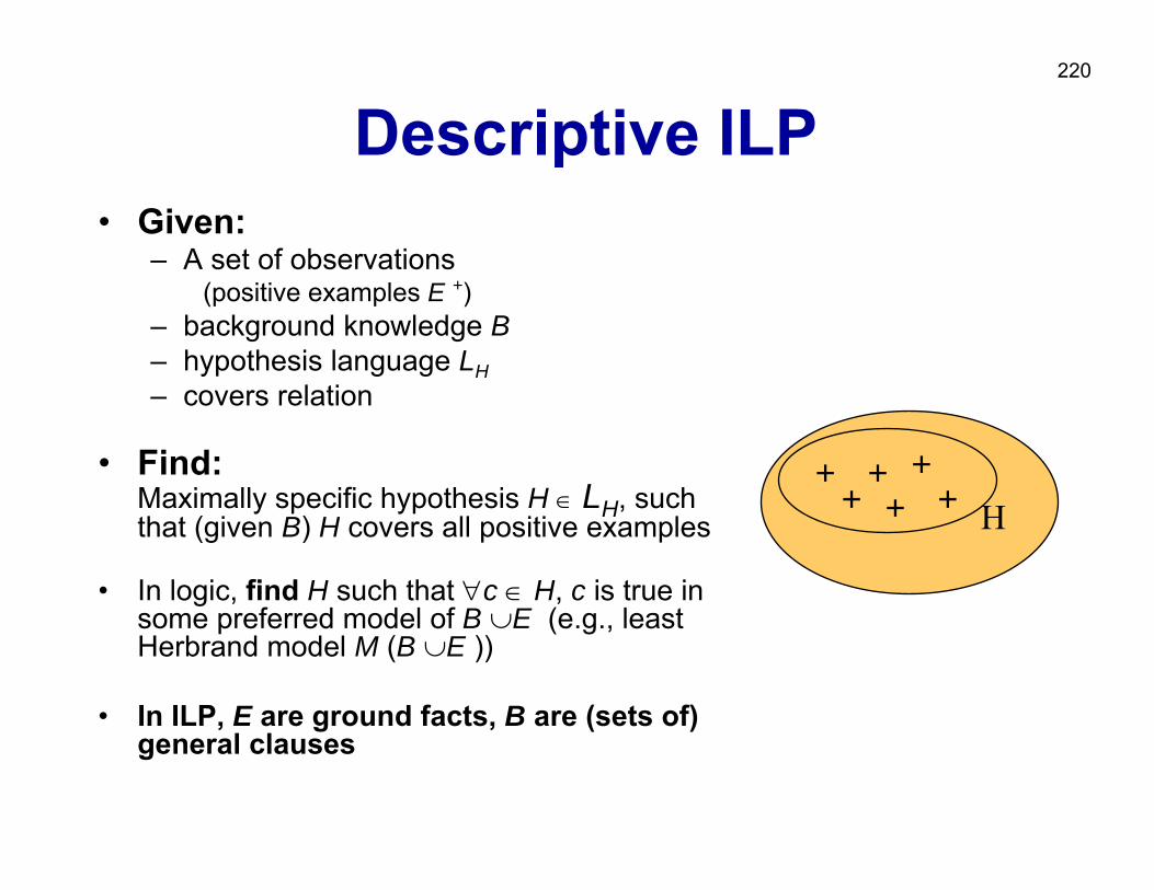
220
Descriptive ILP• Given:
– A set of observations(positive examples E +)
– background knowledge B– hypothesis language LH– covers relation
• Find:Maximally specific hypothesis H ∈ LH, such that (given B) H covers all positive examples
• In logic, find H such that ∀c ∈ H, c is true in some preferred model of B ∪E (e.g., least Herbrand model M (B ∪E ))
• In ILP, E are ground facts, B are (sets of) general clauses
+ + ++++ Η
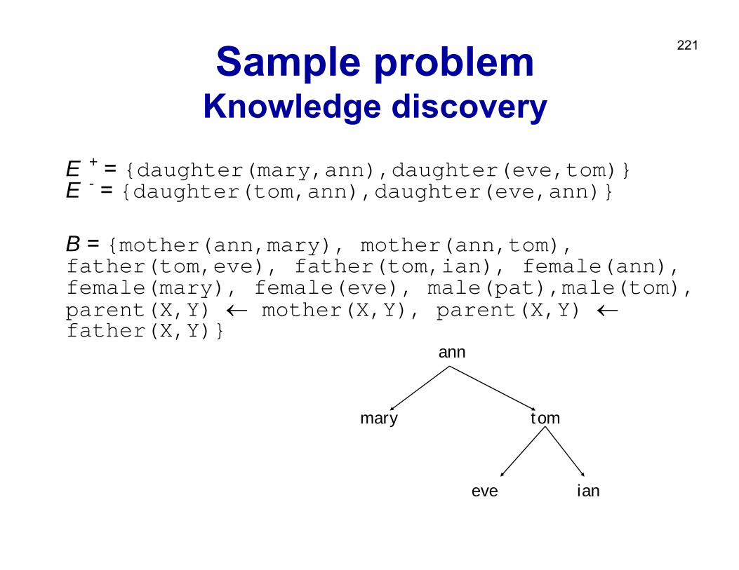
221Sample problemKnowledge discovery
E + = {daughter(mary,ann),daughter(eve,tom)}E - = {daughter(tom,ann),daughter(eve,ann)}
B = {mother(ann,mary), mother(ann,tom), father(tom,eve), father(tom,ian), female(ann), female(mary), female(eve), male(pat),male(tom), parent(X,Y) ← mother(X,Y), parent(X,Y) ←father(X,Y)}
ann
mary tom
eve ian
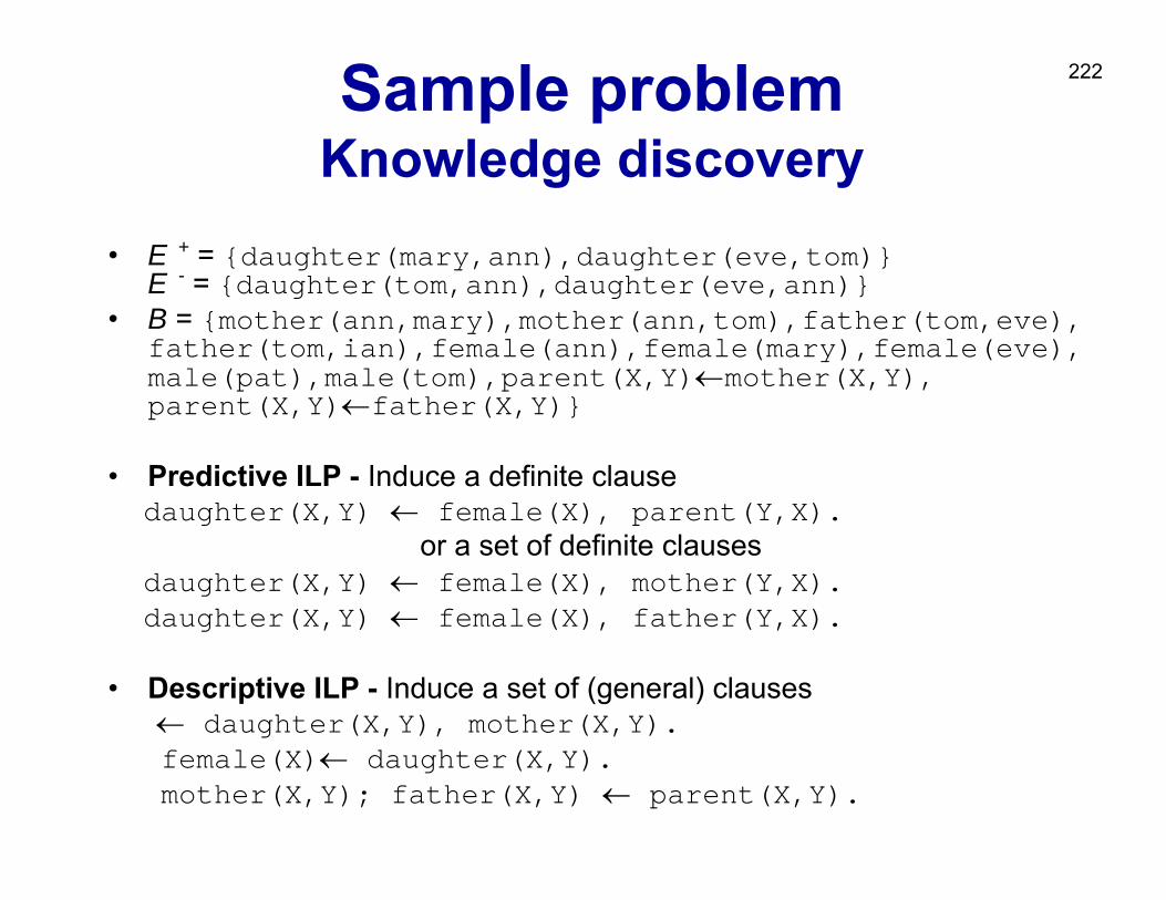
222Sample problemKnowledge discovery
• E + = {daughter(mary,ann),daughter(eve,tom)}E - = {daughter(tom,ann),daughter(eve,ann)}
• B = {mother(ann,mary),mother(ann,tom),father(tom,eve),father(tom,ian),female(ann),female(mary),female(eve),male(pat),male(tom),parent(X,Y)←mother(X,Y),parent(X,Y)←father(X,Y)}
• Predictive ILP - Induce a definite clausedaughter(X,Y) ← female(X), parent(Y,X).
or a set of definite clausesdaughter(X,Y) ← female(X), mother(Y,X).daughter(X,Y) ← female(X), father(Y,X).
• Descriptive ILP - Induce a set of (general) clauses← daughter(X,Y), mother(X,Y).female(X)← daughter(X,Y).mother(X,Y); father(X,Y) ← parent(X,Y).
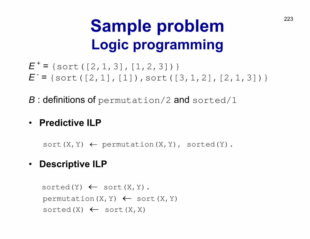
223Sample problemLogic programming
E + = {sort([2,1,3],[1,2,3])}E - = {sort([2,1],[1]),sort([3,1,2],[2,1,3])}
B : definitions of permutation/2 and sorted/1
• Predictive ILP
sort(X,Y) ← permutation(X,Y), sorted(Y).
• Descriptive ILP
sorted(Y) ← sort(X,Y).
permutation(X,Y) ← sort(X,Y)sorted(X) ← sort(X,X)
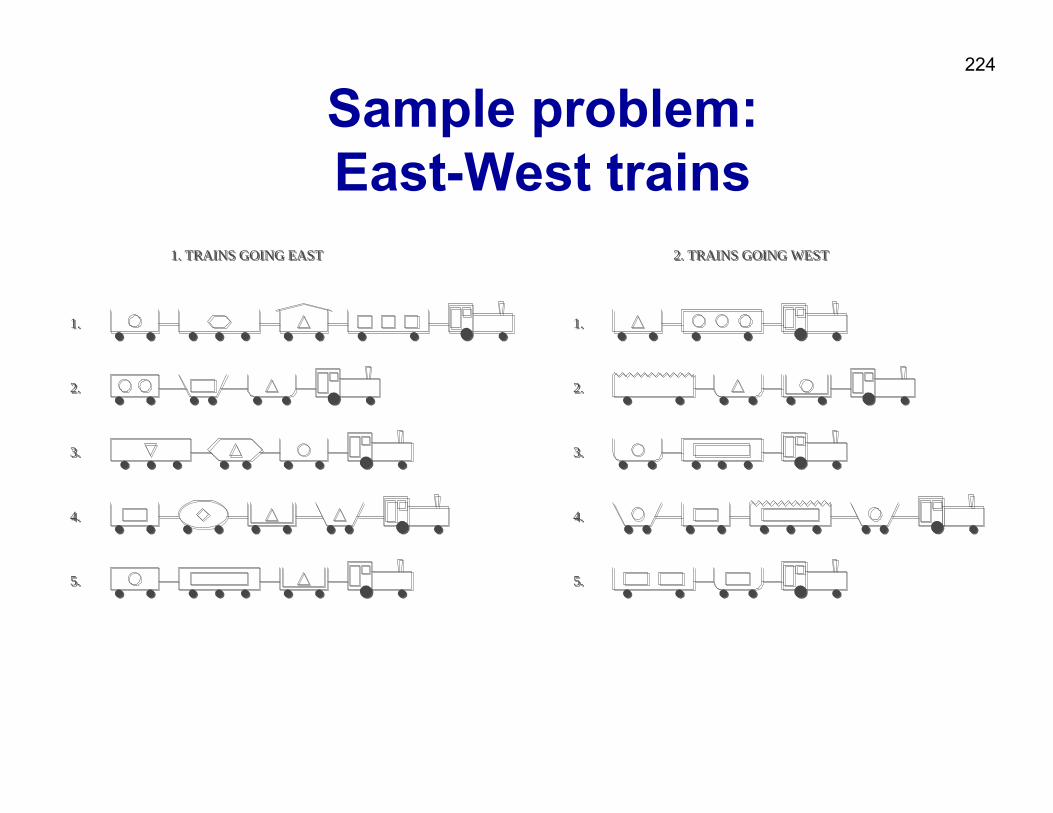
224
Sample problem: East-West trains
1. TRAINS GOING EAST 2. TRAINS GOING WEST
1.
2.
3.
4.
5.
1.
2.
3.
4.
5.
1. TRAINS GOING EAST 2. TRAINS GOING WEST
1.
2.
3.
4.
5.
1.
2.
3.
4.
5.
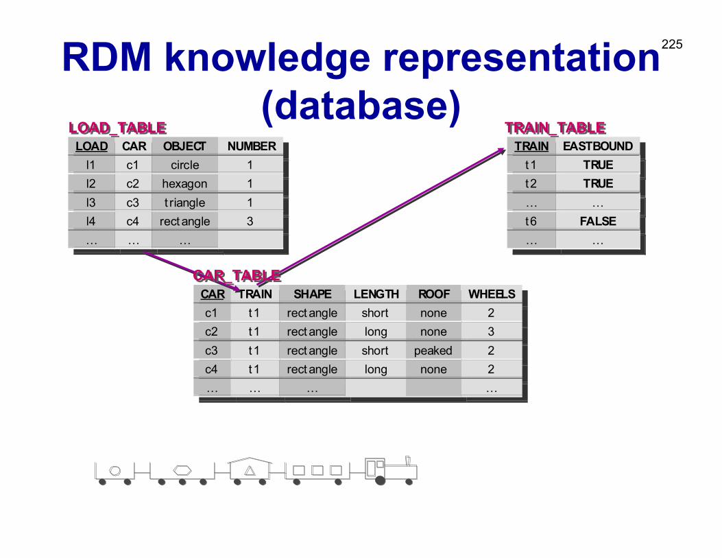
225RDM knowledge representation (database)
TRAIN EASTBOUNDt1 TRUEt2 TRUE… …t6 FALSE… …
TRAIN EASTBOUNDt1 TRUEt2 TRUE… …t6 FALSE… …
TRAIN_TABLETRAIN_TABLE
CAR TRAIN SHAPE LENGTH ROOF WHEELSc1 t1 rect angle short none 2c2 t1 rect angle long none 3c3 t1 rect angle short peaked 2c4 t1 rect angle long none 2… … … …
CAR TRAIN SHAPE LENGTH ROOF WHEELSc1 t1 rect angle short none 2c2 t1 rect angle long none 3c3 t1 rect angle short peaked 2c4 t1 rect angle long none 2… … … …
LOAD CAR OBJECT NUMBERl1 c1 circle 1l2 c2 hexagon 1l3 c3 t riangle 1l4 c4 rect angle 3… … …
LOAD CAR OBJECT NUMBERl1 c1 circle 1l2 c2 hexagon 1l3 c3 t riangle 1l4 c4 rect angle 3… … …
LOAD_TABLELOAD_TABLE
CAR_TABLECAR_TABLE
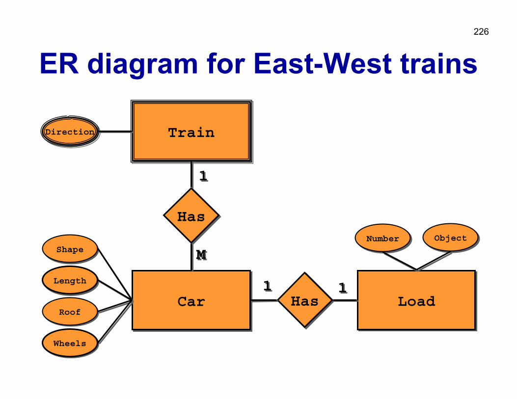
226
ER diagram for East-West trains
TrainTrainDirectionDirection
HasHas
CarCar
ShapeShape
LengthLength
RoofRoof
WheelsWheels
11
MM
HasHas LoadLoad11 11
NumberNumber ObjectObject
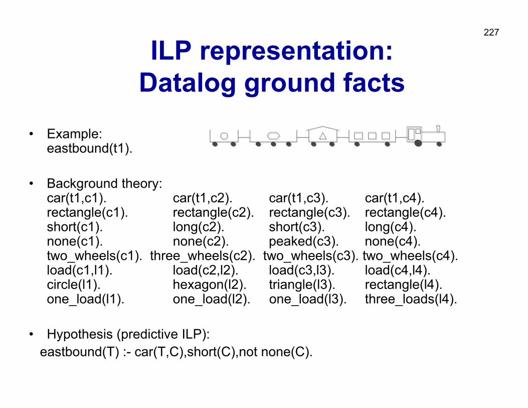
227
ILP representation: Datalog ground facts
• Example: eastbound(t1).
• Background theory:car(t1,c1). car(t1,c2). car(t1,c3). car(t1,c4).rectangle(c1). rectangle(c2). rectangle(c3). rectangle(c4).short(c1). long(c2). short(c3). long(c4).none(c1). none(c2). peaked(c3). none(c4).two_wheels(c1). three_wheels(c2). two_wheels(c3). two_wheels(c4).load(c1,l1). load(c2,l2). load(c3,l3). load(c4,l4).circle(l1). hexagon(l2). triangle(l3). rectangle(l4).one_load(l1). one_load(l2). one_load(l3). three_loads(l4).
• Hypothesis (predictive ILP):eastbound(T) :- car(T,C),short(C),not none(C).
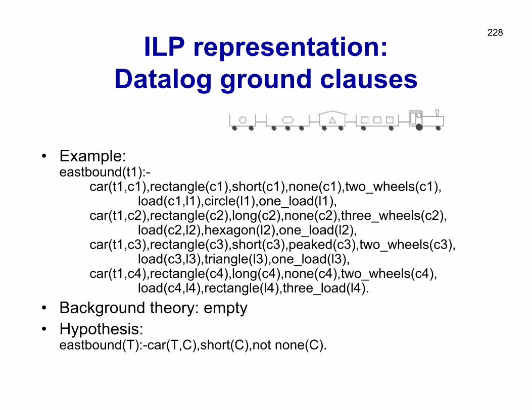
228
ILP representation: Datalog ground clauses
• Example: eastbound(t1):-
car(t1,c1),rectangle(c1),short(c1),none(c1),two_wheels(c1),load(c1,l1),circle(l1),one_load(l1),
car(t1,c2),rectangle(c2),long(c2),none(c2),three_wheels(c2),load(c2,l2),hexagon(l2),one_load(l2),
car(t1,c3),rectangle(c3),short(c3),peaked(c3),two_wheels(c3),load(c3,l3),triangle(l3),one_load(l3),
car(t1,c4),rectangle(c4),long(c4),none(c4),two_wheels(c4),load(c4,l4),rectangle(l4),three_load(l4).
• Background theory: empty • Hypothesis:
eastbound(T):-car(T,C),short(C),not none(C).
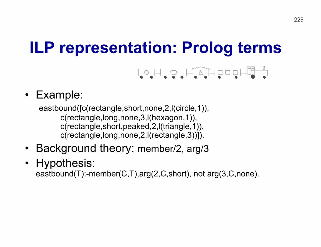
229
ILP representation: Prolog terms
• Example: eastbound([c(rectangle,short,none,2,l(circle,1)),
c(rectangle,long,none,3,l(hexagon,1)),c(rectangle,short,peaked,2,l(triangle,1)),c(rectangle,long,none,2,l(rectangle,3))]).
• Background theory: member/2, arg/3• Hypothesis:
eastbound(T):-member(C,T),arg(2,C,short), not arg(3,C,none).
230
First-order representations
• Propositional representations: – datacase is fixed-size vector of values– features are those given in the dataset
• First-order representations: – datacase is flexible-size, structured object
• sequence, set, graph• hierarchical: e.g. set of sequences
– features need to be selected from potentially infinite set
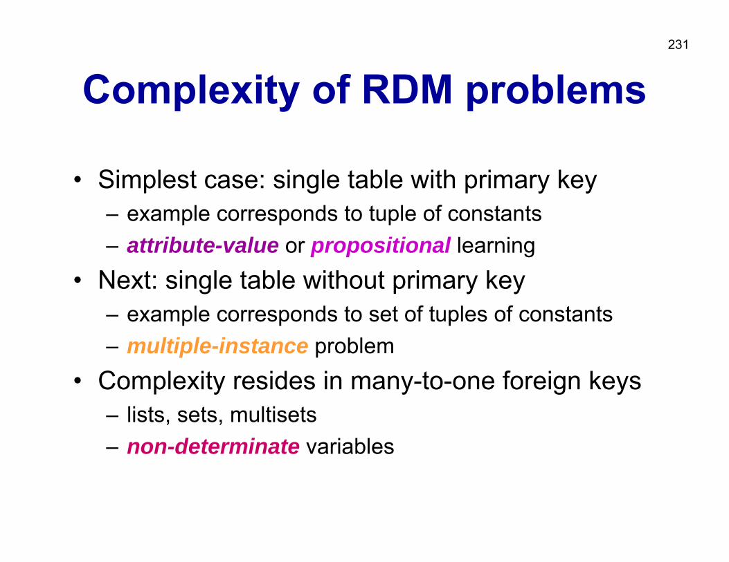
231
Complexity of RDM problems
• Simplest case: single table with primary key– example corresponds to tuple of constants– attribute-value or propositional learning
• Next: single table without primary key– example corresponds to set of tuples of constants– multiple-instance problem
• Complexity resides in many-to-one foreign keys– lists, sets, multisets– non-determinate variables
232Part V: Relational Data Mining
• Learning as search• What is RDM?• Propositionalization techniques• Inductive Logic Programming
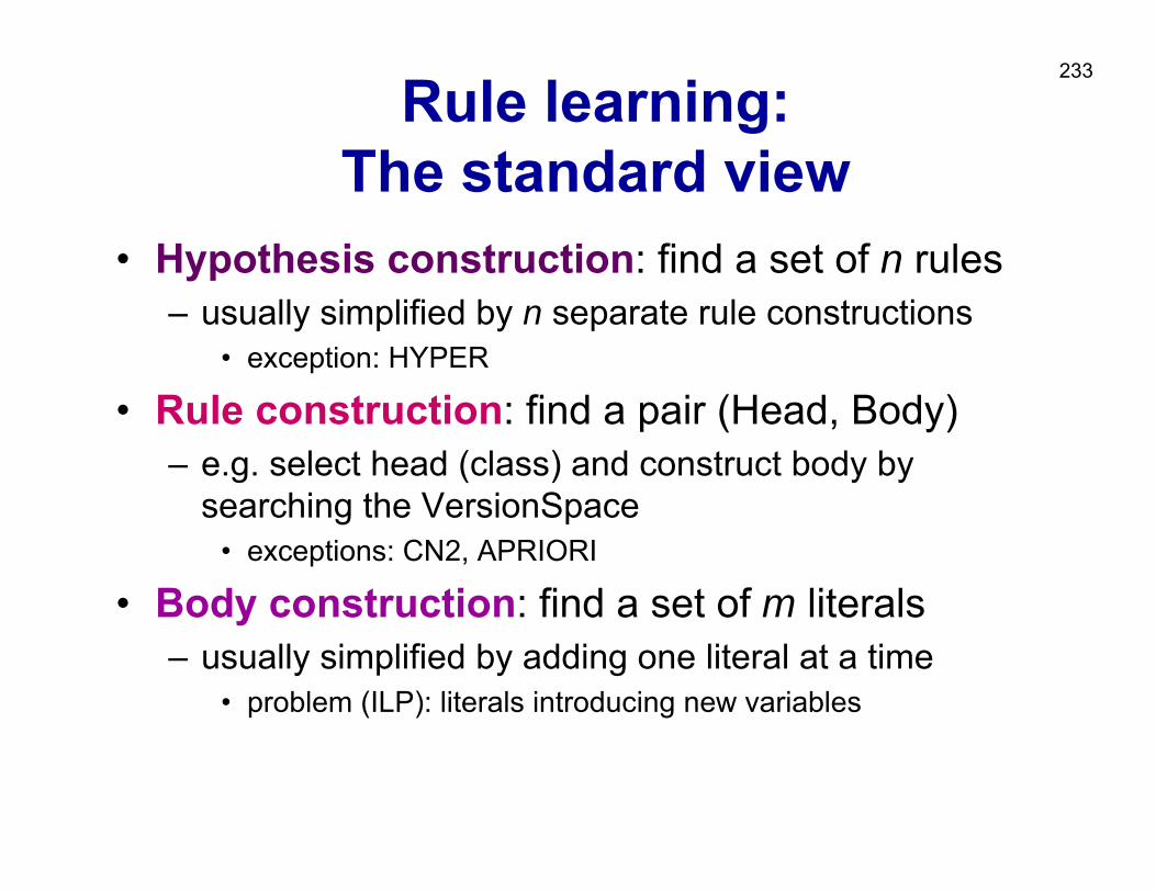
233
Rule learning: The standard view
• Hypothesis construction: find a set of n rules– usually simplified by n separate rule constructions
• exception: HYPER
• Rule construction: find a pair (Head, Body)– e.g. select head (class) and construct body by
searching the VersionSpace• exceptions: CN2, APRIORI
• Body construction: find a set of m literals– usually simplified by adding one literal at a time
• problem (ILP): literals introducing new variables
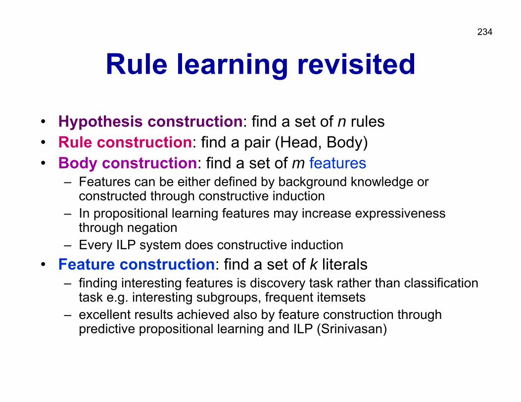
234
Rule learning revisited
• Hypothesis construction: find a set of n rules• Rule construction: find a pair (Head, Body)• Body construction: find a set of m features
– Features can be either defined by background knowledge or constructed through constructive induction
– In propositional learning features may increase expressiveness through negation
– Every ILP system does constructive induction • Feature construction: find a set of k literals
– finding interesting features is discovery task rather than classification task e.g. interesting subgroups, frequent itemsets
– excellent results achieved also by feature construction through predictive propositional learning and ILP (Srinivasan)
235
First-order feature construction
• All the expressiveness of ILP is in the features• Given a way to construct (or choose) first-order
features, body construction in ILP becomes propositional– idea: learn non-determinate clauses with LINUS by
saturating background knowledge (performing systematic feature construction in a given language bias)
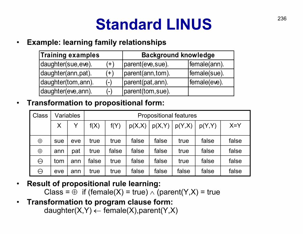
236Standard LINUS• Example: learning family relationships
• Transformation to propositional form:
• Result of propositional rule learning:Class = ⊕ if (female(X) = true) ∧ (parent(Y,X) = true
• Transformation to program clause form:daughter(X,Y) ← female(X),parent(Y,X)
Training examplesdaughter(sue,eve). (+) parent(eve,sue). female(ann).daughter(ann,pat). (+) parent(ann,tom). female(sue).daughter(tom,ann). (-) parent(pat,ann). female(eve).daughter(eve,ann). (-) parent(tom,sue).
Background knowledge
falsefalsefalsefalsefalsetruetrueannevefalsefalsetruefalsefalsetruefalseanntomfalsefalsetruefalsefalsefalsetruepatann⊕
falsefalsetruefalsefalsetruetrueevesue⊕
X=Yp(Y,Y)p(Y,X)p(X,Y)p(X,X)f(Y)f(X)YXPropositional featuresVariablesClass
237
Representation issues (1)• In the database and Datalog ground fact
representations individual examples are not easily separable
• Term and Datalog ground clause representations enable the separation of individuals
• Term representation collects all information about an individual in one structured term
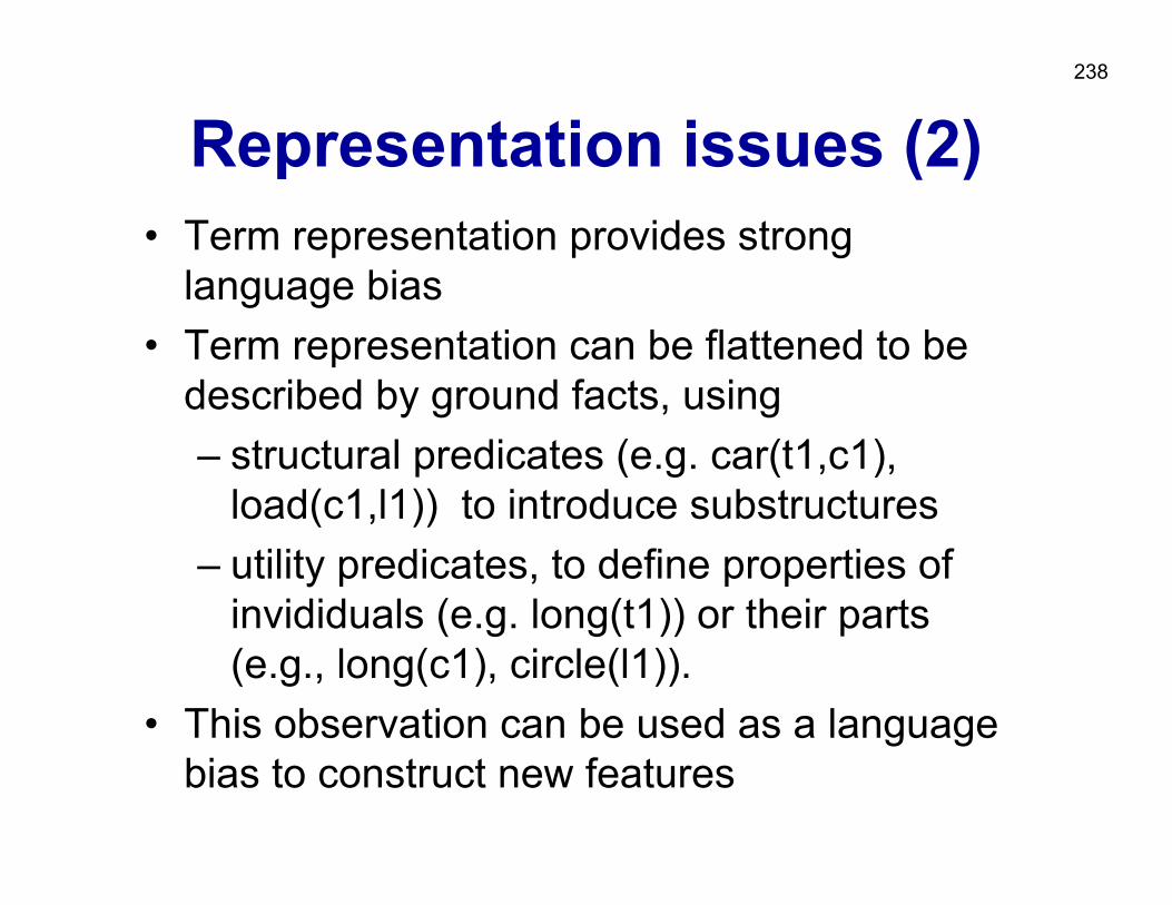
238
Representation issues (2)• Term representation provides strong
language bias• Term representation can be flattened to be
described by ground facts, using– structural predicates (e.g. car(t1,c1),
load(c1,l1)) to introduce substructures– utility predicates, to define properties of
invididuals (e.g. long(t1)) or their parts (e.g., long(c1), circle(l1)).
• This observation can be used as a language bias to construct new features
239
Declarative bias for first-order feature construction
• In ILP, features involve interactions of local variables• Features should define properties of individuals (e.g. trains,
molecules) or their parts (e.g., cars, atoms) • Feature construction in LINUS, using the following language
bias:– one free global variable (denoting an individual, e.g. train)– one or more structural predicates: (e.g., has_car(T,C)) ,each
introducing a new existential local variable (e.g. car, atom), using either the global variable (train, molecule) or a local variable introduced by other structural predicates (car, load)
– one or more utility predicates defining properties of individuals or their parts: no new variables, just using variables
– all variables should be used– parameter: max. number of predicates forming a feature
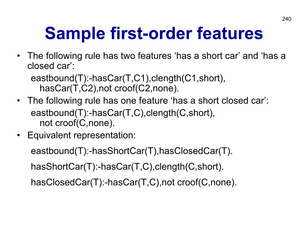
240
Sample first-order features• The following rule has two features ‘has a short car’ and ‘has a
closed car’: eastbound(T):-hasCar(T,C1),clength(C1,short),
hasCar(T,C2),not croof(C2,none).• The following rule has one feature ‘has a short closed car’:
eastbound(T):-hasCar(T,C),clength(C,short),not croof(C,none).
• Equivalent representation:
eastbound(T):-hasShortCar(T),hasClosedCar(T).
hasShortCar(T):-hasCar(T,C),clength(C,short).
hasClosedCar(T):-hasCar(T,C),not croof(C,none).
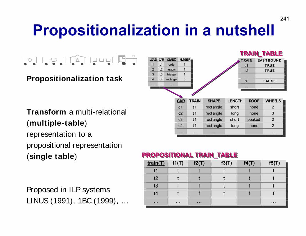
241
Propositionalization in a nutshell
T RAI N EAS T BOUNDt 1 T RUEt 2 T RUE… …t 6 FAL SE… …
T RAI N EAS T BOUNDt 1 T RUEt 2 T RUE… …t 6 FAL SE… …
TRAIN_TABLETRAIN_TABLE
CAR TRAIN SHAPE LENGTH ROOF WHEELSc1 t1 rect angle short none 2c2 t1 rect angle long none 3c3 t1 rect angle short peaked 2c4 t1 rect angle long none 2… … … …
CAR TRAIN SHAPE LENGTH ROOF WHEELSc1 t1 rect angle short none 2c2 t1 rect angle long none 3c3 t1 rect angle short peaked 2c4 t1 rect angle long none 2… … … …
LOAD CAR OBJECT NUMBERl1 c1 circle 1l2 c2 hexagon 1l3 c3 triangle 1l4 c4 rectangle 3… … …
LOAD CAR OBJECT NUMBERl1 c1 circle 1l2 c2 hexagon 1l3 c3 triangle 1l4 c4 rectangle 3… … …
train(T) f1(T) f2(T) f3(T) f4(T) f5(T)t1 t t f t t t2 t t t t t t3 f f t f f t4 t f t f f … … … …
train(T) f1(T) f2(T) f3(T) f4(T) f5(T)t1 t t f t t t2 t t t t t t3 f f t f f t4 t f t f f … … … …
PROPOSITIONAL TRAIN_TABLEPROPOSITIONAL TRAIN_TABLE
Propositionalization task
Transform a multi-relational(multiple-table)representation to a propositional representation(single table)
Proposed in ILP systemsLINUS (1991), 1BC (1999), …
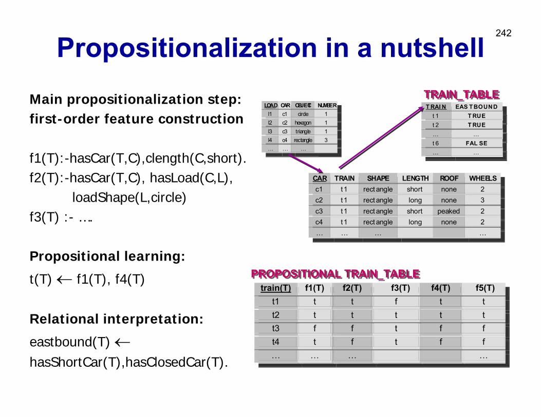
242
Propositionalization in a nutshell
T RAI N EAS T BOUNDt 1 T RUEt 2 T RUE… …t 6 FAL SE… …
T RAI N EAS T BOUNDt 1 T RUEt 2 T RUE… …t 6 FAL SE… …
TRAIN_TABLETRAIN_TABLE
CAR TRAIN SHAPE LENGTH ROOF WHEELSc1 t1 rect angle short none 2c2 t1 rect angle long none 3c3 t1 rect angle short peaked 2c4 t1 rect angle long none 2… … … …
CAR TRAIN SHAPE LENGTH ROOF WHEELSc1 t1 rect angle short none 2c2 t1 rect angle long none 3c3 t1 rect angle short peaked 2c4 t1 rect angle long none 2… … … …
LOAD CAR OBJECT NUMBERl1 c1 circle 1l2 c2 hexagon 1l3 c3 triangle 1l4 c4 rectangle 3… … …
LOAD CAR OBJECT NUMBERl1 c1 circle 1l2 c2 hexagon 1l3 c3 triangle 1l4 c4 rectangle 3… … …
train(T) f1(T) f2(T) f3(T) f4(T) f5(T)t1 t t f t t t2 t t t t t t3 f f t f f t4 t f t f f … … … …
train(T) f1(T) f2(T) f3(T) f4(T) f5(T)t1 t t f t t t2 t t t t t t3 f f t f f t4 t f t f f … … … …
PROPOSITIONAL TRAIN_TABLEPROPOSITIONAL TRAIN_TABLE
Main propositionalization step:first-order feature construction
f1(T):-hasCar(T,C),clength(C,short).f2(T):-hasCar(T,C), hasLoad(C,L),
loadShape(L,circle)f3(T) :- ….
Propositional learning:
t(T) ← f1(T), f4(T)
Relational interpretation:
eastbound(T) ←hasShortCar(T),hasClosedCar(T).
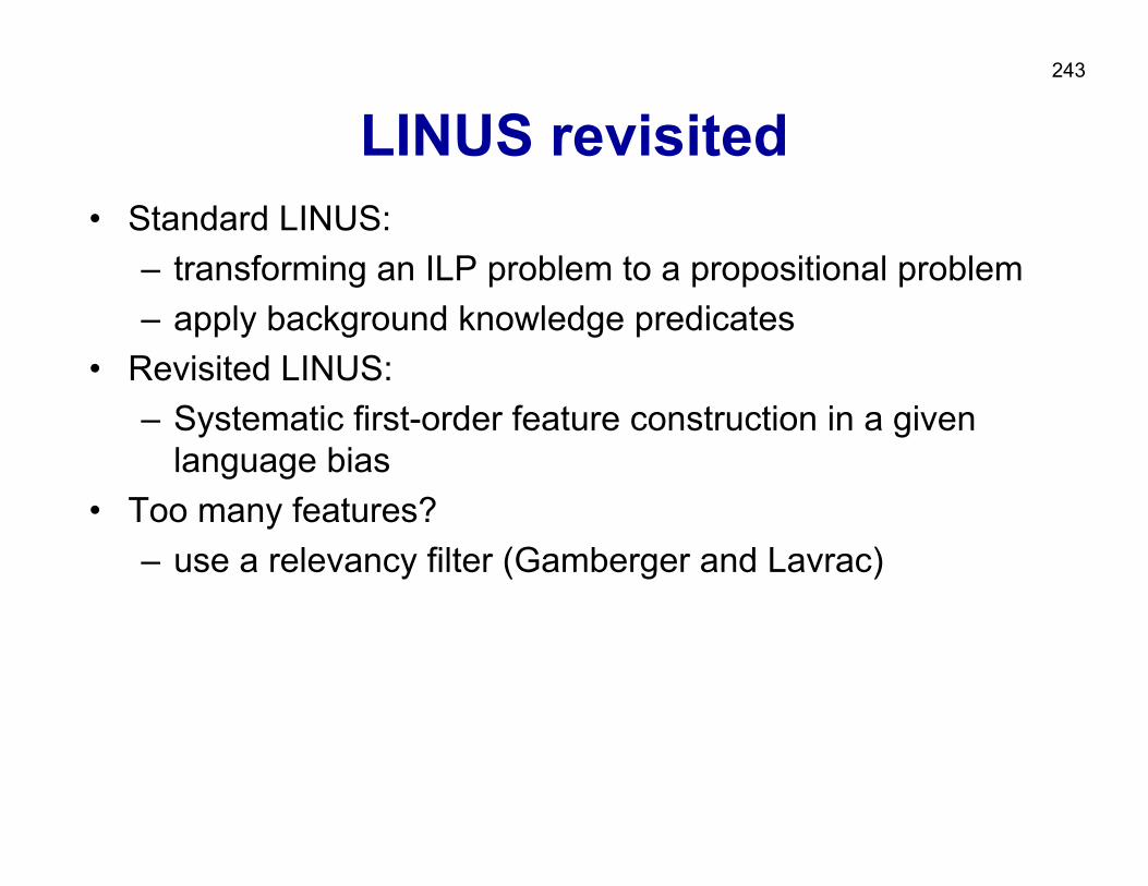
243
LINUS revisited• Standard LINUS:
– transforming an ILP problem to a propositional problem– apply background knowledge predicates
• Revisited LINUS: – Systematic first-order feature construction in a given
language bias• Too many features?
– use a relevancy filter (Gamberger and Lavrac)
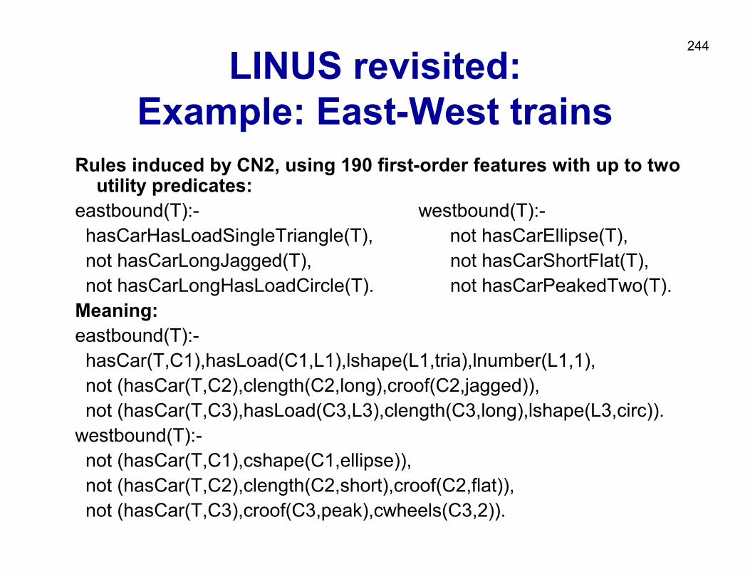
244
LINUS revisited:Example: East-West trains
Rules induced by CN2, using 190 first-order features with up to two utility predicates:
eastbound(T):- westbound(T):-hasCarHasLoadSingleTriangle(T), not hasCarEllipse(T),not hasCarLongJagged(T), not hasCarShortFlat(T),not hasCarLongHasLoadCircle(T). not hasCarPeakedTwo(T).
Meaning:eastbound(T):-hasCar(T,C1),hasLoad(C1,L1),lshape(L1,tria),lnumber(L1,1),not (hasCar(T,C2),clength(C2,long),croof(C2,jagged)),not (hasCar(T,C3),hasLoad(C3,L3),clength(C3,long),lshape(L3,circ)).
westbound(T):-not (hasCar(T,C1),cshape(C1,ellipse)),not (hasCar(T,C2),clength(C2,short),croof(C2,flat)),not (hasCar(T,C3),croof(C3,peak),cwheels(C3,2)).
245Part V: Relational Data Mining
• Learning as search• What is RDM?• Propositionalization techniques• Inductive Logic Programming
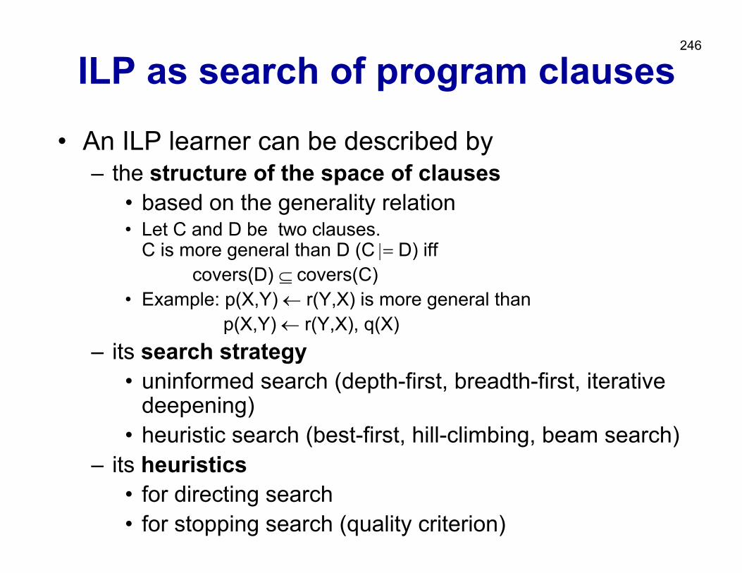
246
ILP as search of program clauses
• An ILP learner can be described by– the structure of the space of clauses
• based on the generality relation • Let C and D be two clauses.
C is more general than D (C |= D) iffcovers(D) ⊆ covers(C)
• Example: p(X,Y) ← r(Y,X) is more general than p(X,Y) ← r(Y,X), q(X)
– its search strategy• uninformed search (depth-first, breadth-first, iterative
deepening)• heuristic search (best-first, hill-climbing, beam search)
– its heuristics• for directing search• for stopping search (quality criterion)
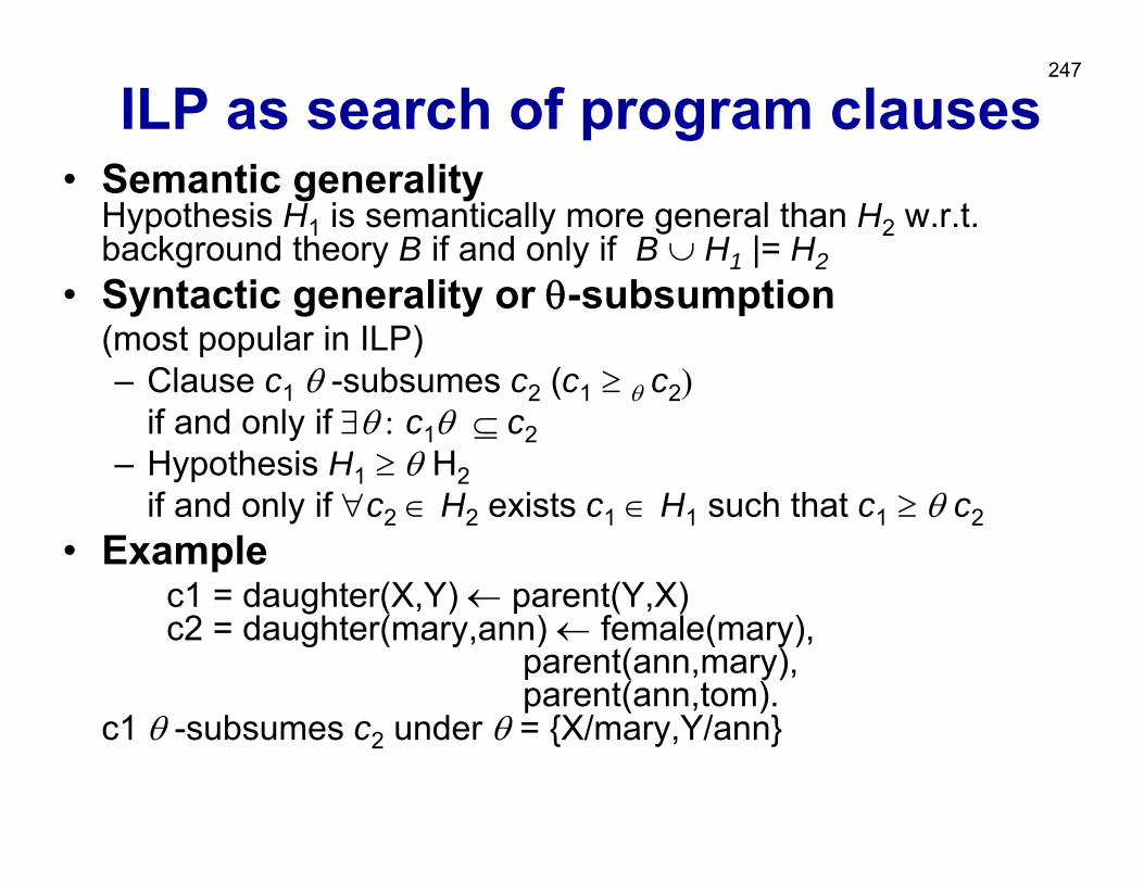
247
• Semantic generalityHypothesis H1 is semantically more general than H2 w.r.t. background theory B if and only if B ∪ H1 |= H2
• Syntactic generality or θ-subsumption(most popular in ILP)– Clause c1 θ -subsumes c2 (c1 ≥ θ c2)
if and only if ∃θ : c1θ ⊆ c2– Hypothesis H1 ≥ θ H2
if and only if ∀c2 ∈ H2 exists c1 ∈ H1 such that c1 ≥ θ c2
• Examplec1 = daughter(X,Y) ← parent(Y,X)c2 = daughter(mary,ann) ← female(mary),
parent(ann,mary),parent(ann,tom).
c1 θ -subsumes c2 under θ = {X/mary,Y/ann}
ILP as search of program clauses
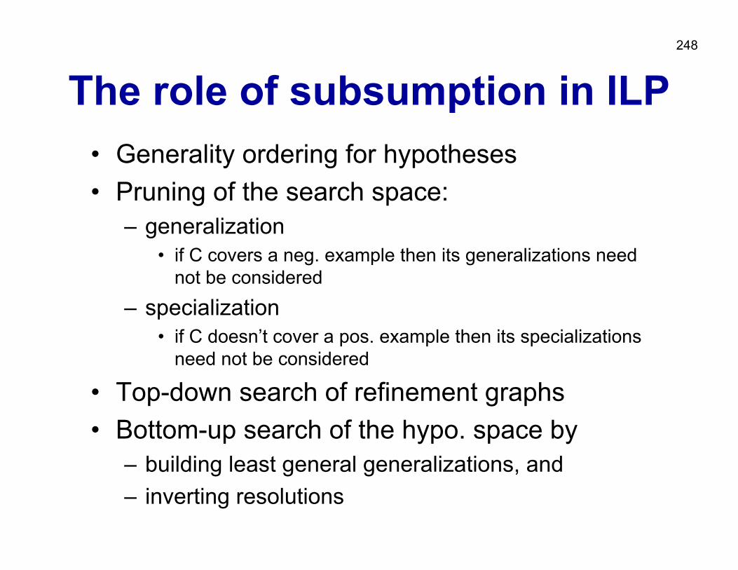
248
The role of subsumption in ILP• Generality ordering for hypotheses• Pruning of the search space:
– generalization• if C covers a neg. example then its generalizations need
not be considered
– specialization• if C doesn’t cover a pos. example then its specializations
need not be considered
• Top-down search of refinement graphs• Bottom-up search of the hypo. space by
– building least general generalizations, and– inverting resolutions
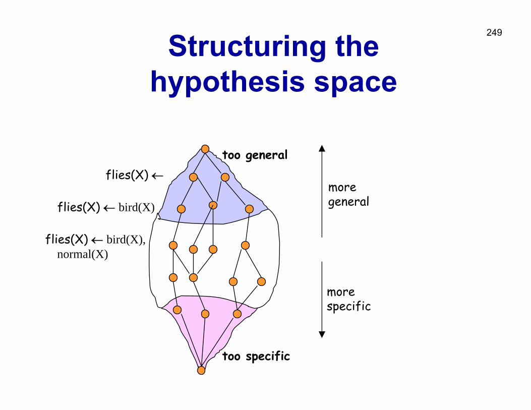
249Structuring the hypothesis space
too general
too specific
moregeneral
morespecific
flies(X) ←
flies(X) ← bird(X), normal(X)
flies(X) ← bird(X)
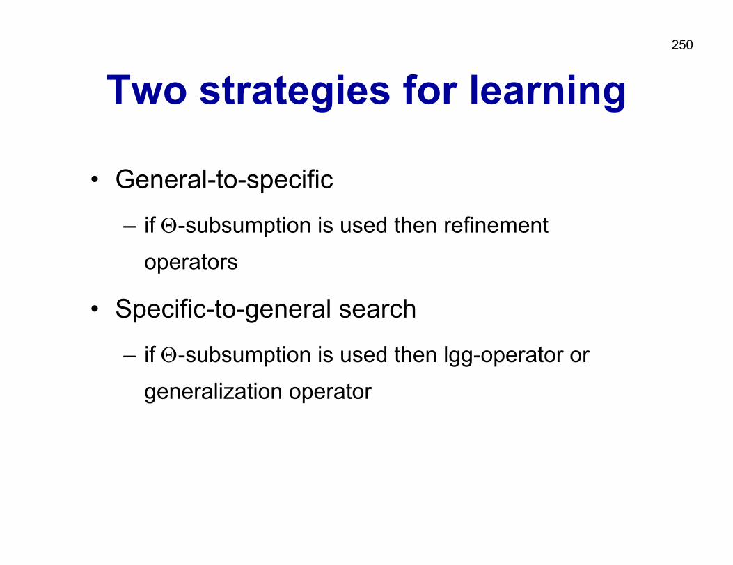
250
Two strategies for learning
• General-to-specific
– if Θ-subsumption is used then refinement operators
• Specific-to-general search
– if Θ-subsumption is used then lgg-operator or generalization operator
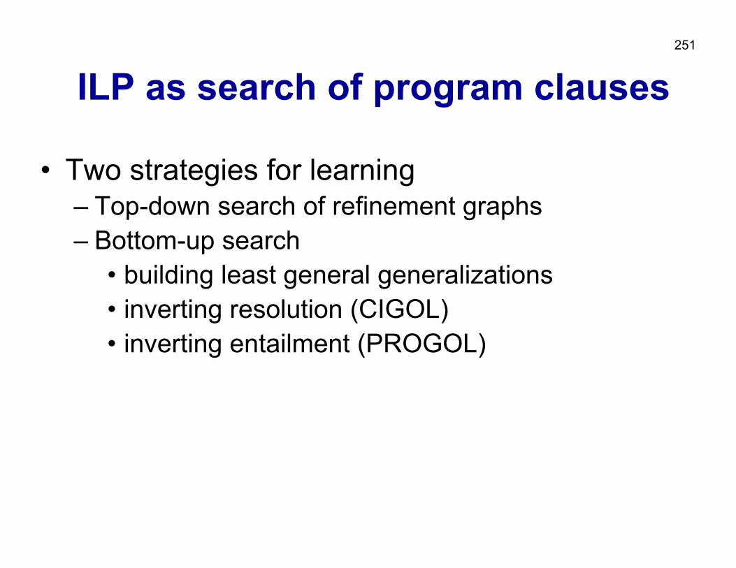
251
• Two strategies for learning– Top-down search of refinement graphs– Bottom-up search
• building least general generalizations• inverting resolution (CIGOL)• inverting entailment (PROGOL)
ILP as search of program clauses
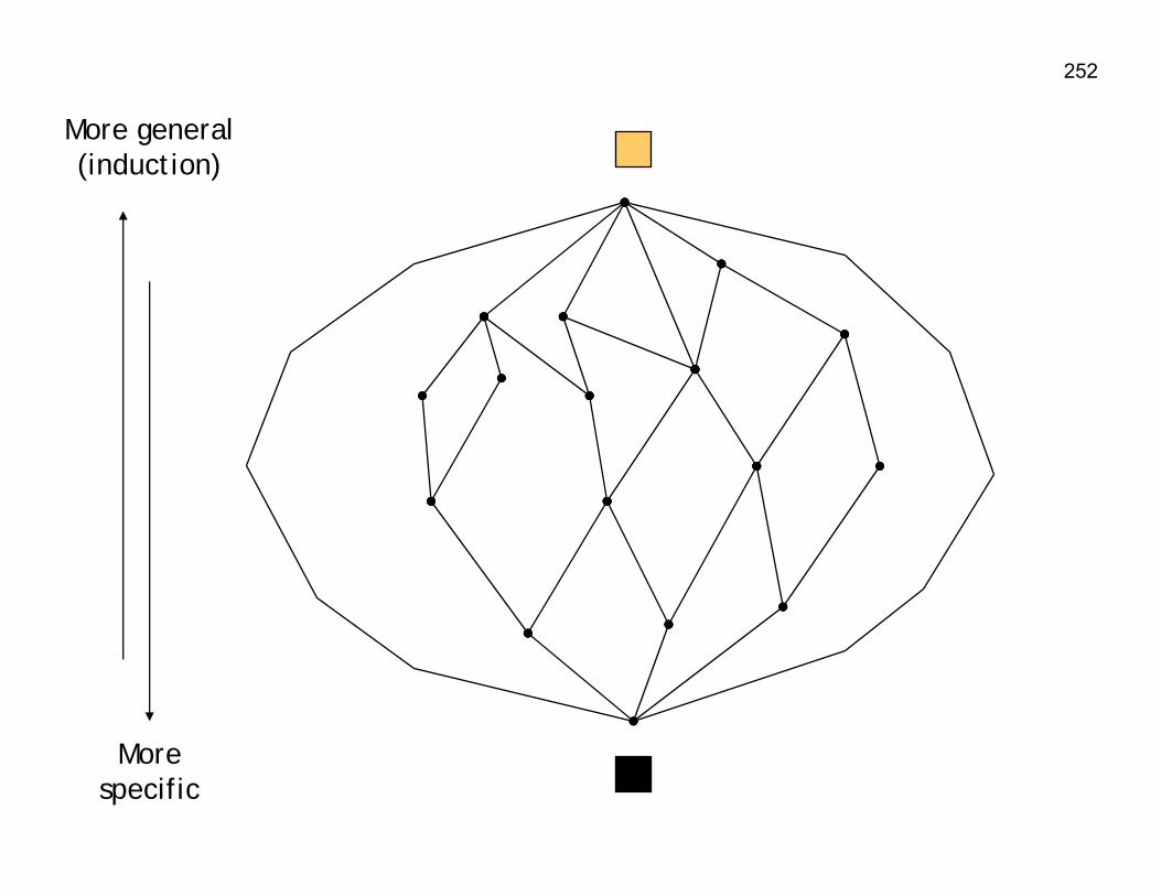
252
More general (induction)
More specific
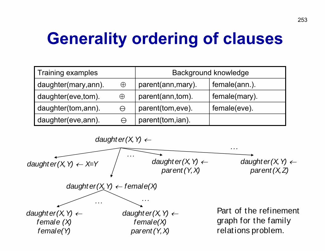
253
Generality ordering of clauses
parent(tom,ian).daughter(eve,ann). female(eve).parent(tom,eve).daughter(tom,ann). female(mary).parent(ann,tom).daughter(eve,tom). ⊕
female(ann.).parent(ann,mary).daughter(mary,ann). ⊕Background knowledgeTraining examples
daughter(X,Y) ←
daughter(X,Y) ← X=Y daughter(X,Y) ←parent(Y,X)
daughter(X,Y) ←parent(X,Z)
daughter(X,Y) ← female(X)
daughter(X,Y) ←female (X)female(Y)
daughter(X,Y) ←female(X)
parent(Y,X)
......
... ...
Part of the refinement graph for the family relations problem.
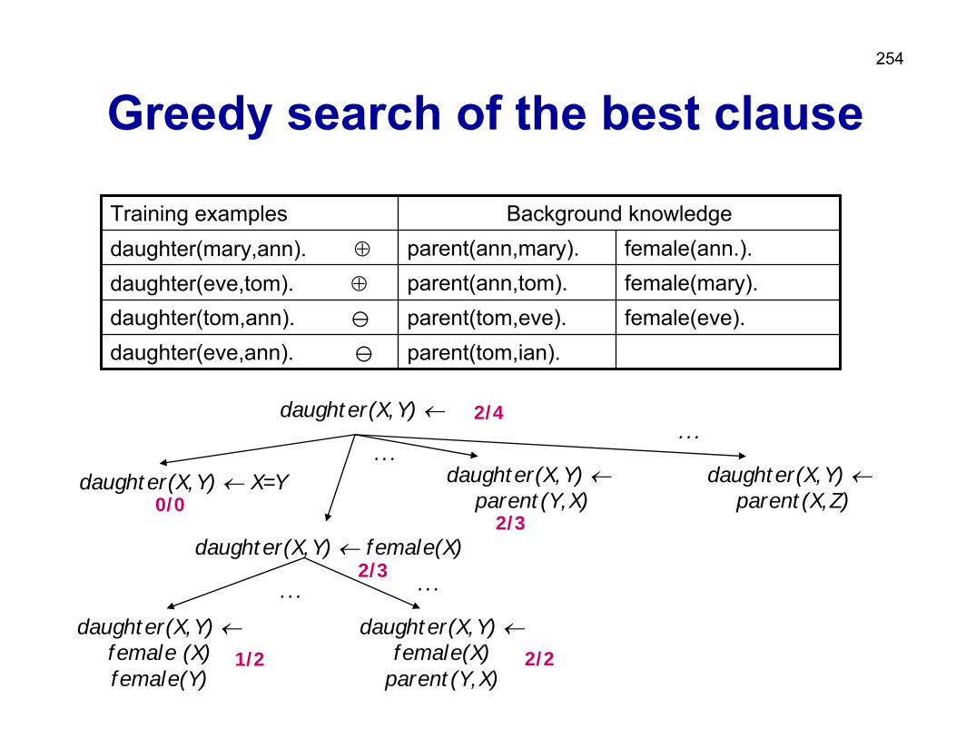
254
Greedy search of the best clause
daughter(X,Y) ←
daughter(X,Y) ← X=Y daughter(X,Y) ←parent(Y,X)
daughter(X,Y) ←parent(X,Z)
daughter(X,Y) ← female(X)
daughter(X,Y) ←female (X)female(Y)
daughter(X,Y) ←female(X)
parent(Y,X)
......
... ...
2/4
0/02/3
2/3
1/2 2/2
parent(tom,ian).daughter(eve,ann). female(eve).parent(tom,eve).daughter(tom,ann). female(mary).parent(ann,tom).daughter(eve,tom). ⊕
female(ann.).parent(ann,mary).daughter(mary,ann). ⊕Background knowledgeTraining examples
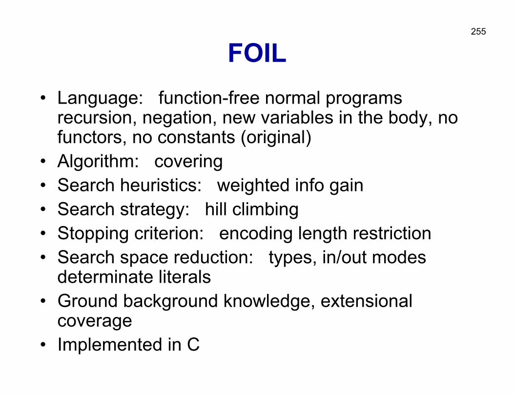
255
FOIL• Language: function-free normal programs
recursion, negation, new variables in the body, no functors, no constants (original)
• Algorithm: covering• Search heuristics: weighted info gain• Search strategy: hill climbing• Stopping criterion: encoding length restriction• Search space reduction: types, in/out modes
determinate literals• Ground background knowledge, extensional
coverage• Implemented in C
256
Part V: Summary
• RDM extends DM by allowing multiple tables describing structured data
• Complexity of representation and therefore of learning is determined by one-to-many links
• Many RDM problems are individual-centred and therefore allow strong declarative bias