knowledge discovery and data mining from big datakumar/presentation/mayo2015/mayo_tutorial... ·...
TRANSCRIPT

Knowledge Discovery and Data
Mining from Big Data
Vipin Kumar
Department of Computer Science
University of Minnesota
[email protected] www.cs.umn.edu/~kumar

July 15, 2015 Mining Big Data ‹#›
Introduction

Mining Big Data: Motivation
Today‟s digital society has seen enormous data growth in both commercial and scientific databases
Data Mining is becoming a commonly used tool to extract information from large and complex datasets
Examples:
Helps provide better customer service in business/commercial setting
Helps scientists in hypothesis formation
Computational Simulations
Business Data
Sensor Networks
Geo-spatial data
Homeland Security
Scientific Data

July 15, 2015 Mining Big Data ‹#›
Data Mining for Life and Health Sciences
Recent technological advances are helping to generate large amounts of both medical and genomic data
• High-throughput experiments/techniques
- Gene and protein sequences
- Gene-expression data
- Biological networks and phylogenetic profiles
• Electronic Medical Records
- IBM-Mayo clinic partnership has created a DB of 5 million patients
- Single Nucleotides Polymorphisms (SNPs)
Data mining offers potential solution for analysis of large-scale data
• Automated analysis of patients history for customized treatment
• Prediction of the functions of anonymous genes
• Identification of putative binding sites in protein structures for drugs/chemicals discovery
Protein Interaction Network
July 15, 2015 Mining Big Data ‹#›
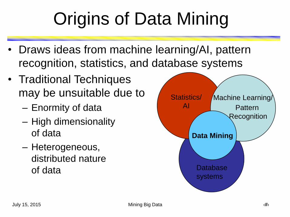
• Draws ideas from machine learning/AI, pattern
recognition, statistics, and database systems
• Traditional Techniques
may be unsuitable due to
– Enormity of data
– High dimensionality
of data
– Heterogeneous,
distributed nature
of data
Origins of Data Mining
Machine Learning/
Pattern
Recognition
Statistics/
AI
Data Mining
Database
systems

July 15, 2015 Mining Big Data ‹#›
Data Mining as Part of the
Knowledge Discovery Process

Data Mining Tasks...
Tid Refund Marital Status
Taxable Income Cheat
1 Yes Single 125K No
2 No Married 100K No
3 No Single 70K No
4 Yes Married 120K No
5 No Divorced 95K Yes
6 No Married 60K No
7 Yes Divorced 220K No
8 No Single 85K Yes
9 No Married 75K No
10 No Single 90K Yes
11 No Married 60K No
12 Yes Divorced 220K No
13 No Single 85K Yes
14 No Married 75K No
15 No Single 90K Yes 10
Milk
Data
July 15, 2015 Mining Big Data ‹#›
Predictive Modeling: Classification

July 15, 2015 Mining Big Data ‹#›
General Approach for Building a
Classification Model
Test
Set
Training
Set Model
Learn
Classifier
Tid Employed Level of
Education
# years at present address
Credit Worthy
1 Yes Graduate 5 Yes
2 Yes High School 2 No
3 No Undergrad 1 No
4 Yes High School 10 Yes
… … … … … 10
Tid Employed Level of
Education
# years at present address
Credit Worthy
1 Yes Undergrad 7 ?
2 No Graduate 3 ?
3 Yes High School 2 ?
… … … … … 10

July 15, 2015 Mining Big Data ‹#›
• Predicting tumor cells as benign or malignant
• Classifying secondary structures of protein as alpha-helix, beta-sheet, or random coil
• Predicting functions of proteins
• Classifying credit card transactions as legitimate or fraudulent
• Categorizing news stories as finance, weather, entertainment, sports, etc
• Identifying intruders in the cyberspace
Examples of Classification Task

July 15, 2015 Mining Big Data ‹#›
Commonly Used Classification Models
• Base Classifiers – Decision Tree based Methods
– Rule-based Methods
– Nearest-neighbor
– Neural Networks
– Naïve Bayes and Bayesian Belief Networks
– Support Vector Machines
• Ensemble Classifiers – Boosting, Bagging, Random Forests
July 15, 2015 Mining Big Data ‹#›
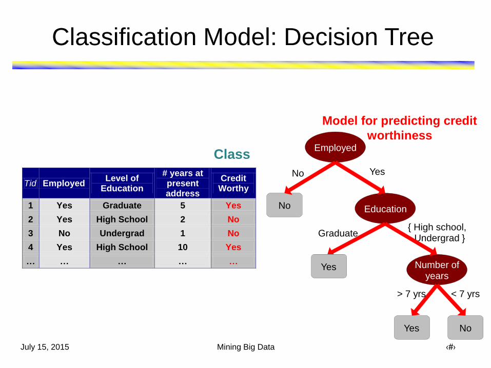
Tid Employed
Level of Education
# years at present address
Credit Worthy
1 Yes Graduate 5 Yes
2 Yes High School 2 No
3 No Undergrad 1 No
4 Yes High School 10 Yes
… … … … … 10
Class
Model for predicting credit
worthiness Employed
No Education
Number of years
No Yes
Graduate { High school, Undergrad }
Yes No
> 7 yrs < 7 yrs
Yes
Classification Model: Decision Tree

July 15, 2015 Mining Big Data ‹#›
Constructing a Decision Tree
10
Tid Employed Level of
Education
# years at present address
Credit Worthy
1 Yes Graduate 5 Yes
2 Yes High School 2 No
3 No Undergrad 1 No
4 Yes High School 10 Yes
5 Yes Graduate 2 No
6 No High School 2 No
7 Yes Undergrad 3 No
8 Yes Graduate 8 Yes
9 Yes High School 4 Yes
10 No Graduate 1 No
Employed
Worthy: 4
Not Worthy: 3
Yes
10
Tid Employed Level of
Education
# years at present address
Credit Worthy
1 Yes Graduate 5 Yes
2 Yes High School 2 No
3 No Undergrad 1 No
4 Yes High School 10 Yes
5 Yes Graduate 2 No
6 No High School 2 No
7 Yes Undergrad 3 No
8 Yes Graduate 8 Yes
9 Yes High School 4 Yes
10 No Graduate 1 No
No
Worthy: 0
Not Worthy: 3
10
Tid Employed Level of
Education
# years at present address
Credit Worthy
1 Yes Graduate 5 Yes
2 Yes High School 2 No
3 No Undergrad 1 No
4 Yes High School 10 Yes
5 Yes Graduate 2 No
6 No High School 2 No
7 Yes Undergrad 3 No
8 Yes Graduate 8 Yes
9 Yes High School 4 Yes
10 No Graduate 1 No
Graduate High School/
Undergrad
Worthy: 2
Not Worthy: 2
Education
Worthy: 2
Not Worthy: 4
Key Computation
Worthy Not
Worthy
4 3
0 3
Employed = Yes
Employed = No
10
Tid Employed Level of
Education
# years at present address
Credit Worthy
1 Yes Graduate 5 Yes
2 Yes High School 2 No
3 No Undergrad 1 No
4 Yes High School 10 Yes
5 Yes Graduate 2 No
6 No High School 2 No
7 Yes Undergrad 3 No
8 Yes Graduate 8 Yes
9 Yes High School 4 Yes
10 No Graduate 1 No
Worthy: 4
Not Worthy: 3
Yes No
Worthy: 0
Not Worthy: 3
Employed

July 15, 2015 Mining Big Data ‹#›
Constructing a Decision Tree
Employed
= Yes
Employed
= No
10
Tid Employed Level of
Education
# years at present address
Credit Worthy
1 Yes Graduate 5 Yes
2 Yes High School 2 No
3 No Undergrad 1 No
4 Yes High School 10 Yes
5 Yes Graduate 2 No
6 No High School 2 No
7 Yes Undergrad 3 No
8 Yes Graduate 8 Yes
9 Yes High School 4 Yes
10 No Graduate 1 No
10
Tid Employed Level of
Education
# years at present address
Credit Worthy
1 Yes Graduate 5 Yes
2 Yes High School 2 No
4 Yes High School 10 Yes
5 Yes Graduate 2 No
7 Yes Undergrad 3 No
8 Yes Graduate 8 Yes
9 Yes High School 4 Yes
10
Tid Employed Level of
Education
# years at present address
Credit Worthy
3 No Undergrad 1 No
6 No High School 2 No
10 No Graduate 1 No

July 15, 2015 Mining Big Data ‹#›
Design Issues of Decision Tree Induction
• How should training records be split?
– Method for specifying test condition
• depending on attribute types
– Measure for evaluating the goodness of a test
condition
• How should the splitting procedure stop?
– Stop splitting if all the records belong to the same
class or have identical attribute values
– Early termination

July 15, 2015 Mining Big Data ‹#›
How to determine the Best Split
Greedy approach:
– Nodes with purer class distribution are
preferred
Need a measure of node impurity:
C0: 5
C1: 5
C0: 9
C1: 1
High degree of impurity Low degree of impurity
July 15, 2015 Mining Big Data ‹#›
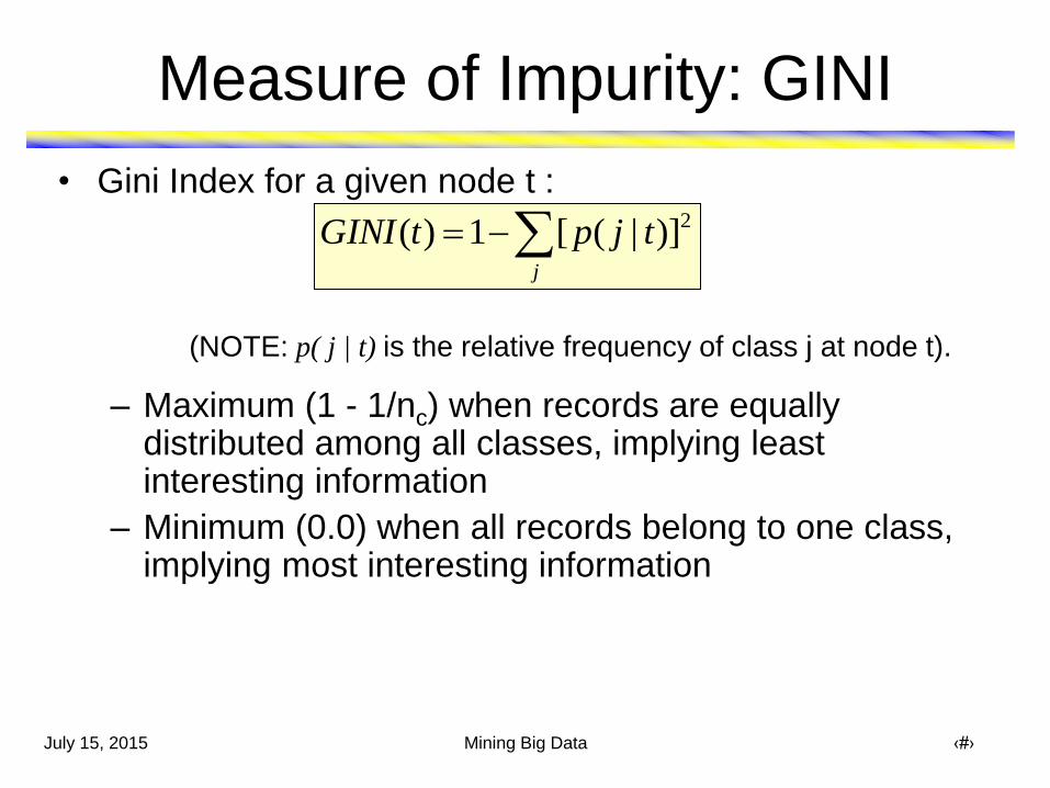
Measure of Impurity: GINI
• Gini Index for a given node t :
(NOTE: p( j | t) is the relative frequency of class j at node t).
– Maximum (1 - 1/nc) when records are equally distributed among all classes, implying least interesting information
– Minimum (0.0) when all records belong to one class, implying most interesting information
j
tjptGINI 2)]|([1)(

July 15, 2015 Mining Big Data ‹#›
Measure of Impurity: GINI
• Gini Index for a given node t :
(NOTE: p( j | t) is the relative frequency of class j at node t).
– For 2-class problem (p, 1 – p): • GINI = 1 – p2 – (1 – p)2 = 2p (1-p)
j
tjptGINI 2)]|([1)(
C1 0
C2 6
Gini=0.000
C1 2
C2 4
Gini=0.444
C1 3
C2 3
Gini=0.500
C1 1
C2 5
Gini=0.278

July 15, 2015 Mining Big Data ‹#›
Computing Gini Index of a Single Node
C1 0
C2 6
C1 2
C2 4
C1 1
C2 5
P(C1) = 0/6 = 0 P(C2) = 6/6 = 1
Gini = 1 – P(C1)2 – P(C2)2 = 1 – 0 – 1 = 0
j
tjptGINI 2)]|([1)(
P(C1) = 1/6 P(C2) = 5/6
Gini = 1 – (1/6)2 – (5/6)2 = 0.278
P(C1) = 2/6 P(C2) = 4/6
Gini = 1 – (2/6)2 – (4/6)2 = 0.444
July 15, 2015 Mining Big Data ‹#›
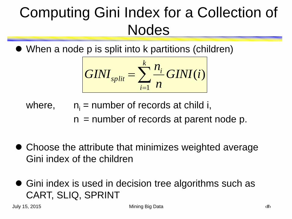
Computing Gini Index for a Collection of
Nodes
When a node p is split into k partitions (children)
where, ni = number of records at child i,
n = number of records at parent node p.
Choose the attribute that minimizes weighted average
Gini index of the children
Gini index is used in decision tree algorithms such as
CART, SLIQ, SPRINT
k
i
isplit iGINI
n
nGINI
1
)(
July 15, 2015 Mining Big Data ‹#›
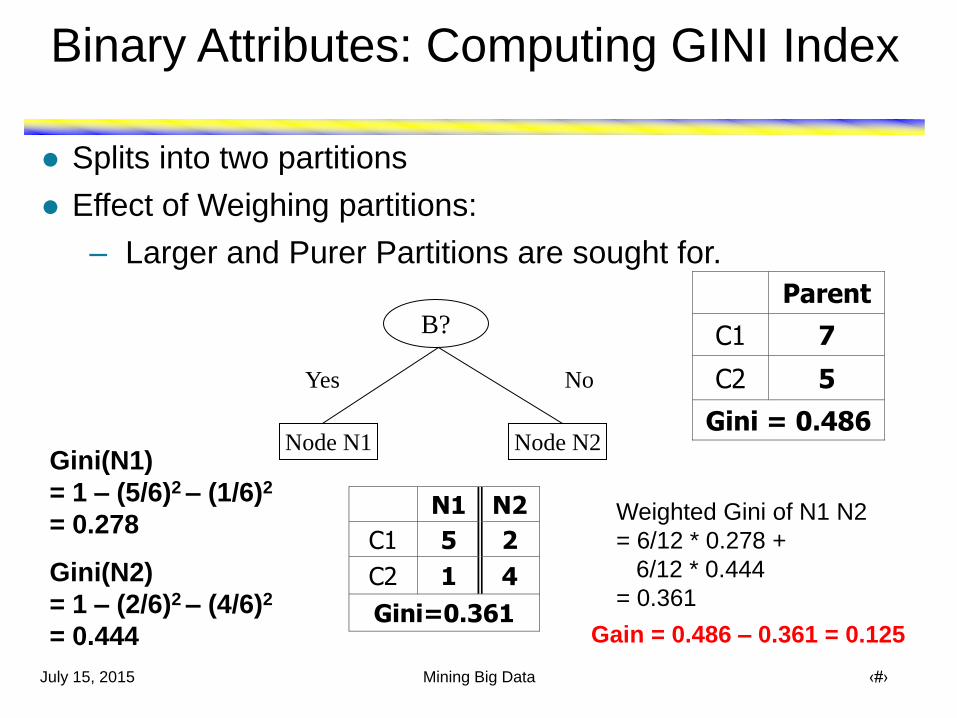
Binary Attributes: Computing GINI Index
Splits into two partitions
Effect of Weighing partitions:
– Larger and Purer Partitions are sought for.
B?
Yes No
Node N1 Node N2
Parent
C1 7
C2 5
Gini = 0.486
N1 N2
C1 5 2
C2 1 4
Gini=0.361
Gini(N1)
= 1 – (5/6)2 – (1/6)2
= 0.278
Gini(N2)
= 1 – (2/6)2 – (4/6)2
= 0.444
Weighted Gini of N1 N2
= 6/12 * 0.278 +
6/12 * 0.444
= 0.361
Gain = 0.486 – 0.361 = 0.125

July 15, 2015 Mining Big Data ‹#›
Continuous Attributes: Computing Gini Index
Use Binary Decisions based on one value
Several Choices for the splitting value
– Number of possible splitting values = Number of distinct values
Each splitting value has a count matrix associated with it
– Class counts in each of the partitions, A < v and A v
Simple method to choose best v
– For each v, scan the database to gather count matrix and compute its Gini index
– Computationally Inefficient! Repetition of work.
ID Home Owner
Marital Status
Annual Income
Defaulted
1 Yes Single 125K No
2 No Married 100K No
3 No Single 70K No
4 Yes Married 120K No
5 No Divorced 95K Yes
6 No Married 60K No
7 Yes Divorced 220K No
8 No Single 85K Yes
9 No Married 75K No
10 No Single 90K Yes 10
Annual
Income
> 80K?
Yes No
≤ 80 > 80
Yes 0 3
No 3 4

July 15, 2015 Mining Big Data ‹#›
Decision Tree Based Classification
Advantages:
– Inexpensive to construct
– Extremely fast at classifying unknown records
– Easy to interpret for small-sized trees
– Robust to noise (especially when methods to avoid
overfitting are employed)
– Can easily handle redundant or irrelevant attributes (unless
the attributes are interacting)
Disadvantages:
– Space of possible decision trees is exponentially large.
Greedy approaches are often unable to find the best tree.
– Does not take into account interactions between attributes
– Each decision boundary involves only a single attribute

July 15, 2015 Mining Big Data ‹#›
Handling interactions
X
Y
+ : 1000 instances
o : 1000 instances
Entropy (X) : 0.99
Entropy (Y) : 0.99

July 15, 2015 Mining Big Data ‹#›
Handling interactions + : 1000 instances
o : 1000 instances
Adding Z as a noisy
attribute generated
from a uniform
distribution
Y
Z
Y
Z
X
Entropy (X) : 0.99
Entropy (Y) : 0.99
Entropy (Z) : 0.98
Attribute Z will be
chosen for splitting!
X

July 15, 2015 Mining Big Data ‹#›
Limitations of single attribute-based decision boundaries
Both positive (+) and
negative (o) classes
generated from
skewed Gaussians
with centers at (8,8)
and (12,12)
respectively.
July 15, 2015 Mining Big Data ‹#›
Model Overfitting
July 15, 2015 Mining Big Data ‹#›
Classification Errors
• Training errors (apparent errors)
– Errors committed on the training set
• Test errors
– Errors committed on the test set
• Generalization errors
– Expected error of a model over random
selection of records from same distribution

July 15, 2015 Mining Big Data ‹#›
Example Data Set
Two class problem:
+ : 5200 instances
• 5000 instances generated from
a Gaussian centered at (10,10)
• 200 noisy instances added
o : 5200 instances
• Generated from a uniform
distribution
10 % of the data used for
training and 90% of the
data used for testing

July 15, 2015 Mining Big Data ‹#›
Increasing number of nodes in
Decision Trees

July 15, 2015 Mining Big Data ‹#›
Decision Tree with 4 nodes
Decision Tree
Decision boundaries on Training data

July 15, 2015 Mining Big Data ‹#›
Decision Tree with 50 nodes
Decision Tree Decision Tree
Decision boundaries on Training data

July 15, 2015 Mining Big Data ‹#›
Which tree is better?
Decision Tree with 4 nodes
Decision Tree with 50 nodes
Which tree is better ?

July 15, 2015 Mining Big Data ‹#›
Model Overfitting
Underfitting: when model is too simple, both training and test errors are large
Overfitting: when model is too complex, training error is small but test error is large

July 15, 2015 Mining Big Data ‹#›
Model Overfitting
Using twice the number of data instances
• If training data is under-representative, testing errors increase and training errors
decrease on increasing number of nodes
• Increasing the size of training data reduces the difference between training and
testing errors at a given number of nodes

July 15, 2015 Mining Big Data ‹#›
Reasons for Model Overfitting
• Presence of Noise
• Lack of Representative Samples
• Multiple Comparison Procedure

July 15, 2015 Mining Big Data ‹#›
Effect of Multiple Comparison
Procedure
• Consider the task of predicting whether
stock market will rise/fall in the next 10
trading days
• Random guessing:
P(correct) = 0.5
• Make 10 random guesses in a row:
Day 1 Up
Day 2 Down
Day 3 Down
Day 4 Up
Day 5 Down
Day 6 Down
Day 7 Up
Day 8 Up
Day 9 Up
Day 10 Down
0547.02
10
10
9
10
8
10
)8(#10
correctP

July 15, 2015 Mining Big Data ‹#›
Effect of Multiple Comparison
Procedure
• Approach:
– Get 50 analysts
– Each analyst makes 10 random guesses
– Choose the analyst that makes the most
number of correct predictions
• Probability that at least one analyst makes
at least 8 correct predictions 9399.0)0547.01(1)8(# 50 correctP

July 15, 2015 Mining Big Data ‹#›
Effect of Multiple Comparison
Procedure
• Many algorithms employ the following greedy strategy:
– Initial model: M
– Alternative model: M‟ = M , where is a component to be added to the model (e.g., a test condition of a decision tree)
– Keep M‟ if improvement, (M,M‟) >
• Often times, is chosen from a set of alternative components, = {1, 2, …, k}
• If many alternatives are available, one may inadvertently add irrelevant components to the model, resulting in model overfitting

July 15, 2015 Mining Big Data ‹#›
Effect of Multiple Comparison - Example
Use additional 100 noisy variables
generated from a uniform distribution
along with X and Y as attributes.
Use 30% of the data for training and
70% of the data for testing Using only X and Y as attributes

July 15, 2015 Mining Big Data ‹#›
Notes on Overfitting
• Overfitting results in decision trees that are
more complex than necessary
• Training error does not provide a good
estimate of how well the tree will perform
on previously unseen records
• Need ways for incorporating model
complexity into model development

July 15, 2015 Mining Big Data ‹#›
Evaluating Performance of Classifier
• Model Selection
– Performed during model building
– Purpose is to ensure that model is not overly complex (to avoid overfitting)
• Model Evaluation
– Performed after model has been constructed
– Purpose is to estimate performance of classifier on previously unseen data (e.g., test set)

July 15, 2015 Mining Big Data ‹#›
Methods for Classifier Evaluation
• Holdout
– Reserve k% for training and (100-k)% for testing
• Random subsampling
– Repeated holdout
• Cross validation
– Partition data into k disjoint subsets
– k-fold: train on k-1 partitions, test on the remaining one
– Leave-one-out: k=n
• Bootstrap
– Sampling with replacement
– .632 bootstrap:
b
i
siboot accaccb
acc1
368.0632.01

July 15, 2015 Mining Big Data ‹#›
Application on Biomedical Data

July 15, 2015 Mining Big Data ‹#›
Application : SNP Association Study
• Given: A patient data set that has genetic variations
(SNPs) and their associated Phenotype (Disease).
• Objective: Finding a combination of genetic
characteristics that best defines the phenotype under
study.
SNP1 SNP2 … SNPM Disease
Patient 1 1 1 … 1 1
Patient 2 0 1 … 1 1
Patient 3 1 0 … 0 0
… … … … … …
Patient N 1 1 1 1
Genetic Variation in Patients (SNPs) as Binary Matrix
and Survival/Disease (Yes/No) as Class Label. Genetic Variation in Patients (SNPs) as Binary Matrix
and Survival/Disease (Yes/No) as Class Label.
Genetic Variation in Patients (SNPs) as Binary Matrix and
Survival/Disease (Yes/No) as Class Label.

July 15, 2015 Mining Big Data ‹#›
SNP (Single nucleotide polymorphism)
• Definition of SNP (wikipedia)
– A SNP is defined as a single base change in a DNA sequence that occurs in a significant proportion (more than 1 percent) of a large population
– How many SNPs in Human genome?
– 10,000,000
Individual 1 A G C G T G A T C G A G G C T A
Individual 2 A G C G T G A T C G A G G C T A
Individual 3 A G C G T G A G C G A G G C T A
Individual 4 A G C G T G A T C G A G G C T A
Individual 5 A G C G T G A T C G A G G C T A
SNP
Each SNP has 3 values
( GG / GT / TT )
( mm / Mm/ MM)

July 15, 2015 Mining Big Data ‹#›
Why is SNPs interesting?
• In human beings, 99.9 percent bases are same.
• Remaining 0.1 percent makes a person unique.
– Different attributes / characteristics / traits • how a person looks,
• diseases a person develops.
• These variations can be: – Harmless (change in phenotype)
– Harmful (diabetes, cancer, heart disease, Huntington's disease, and hemophilia )
– Latent (variations found in coding and regulatory regions, are not harmful on their own, and the change in each gene only becomes apparent under certain conditions e.g. susceptibility to lung cancer)
July 15, 2015 Mining Big Data ‹#›
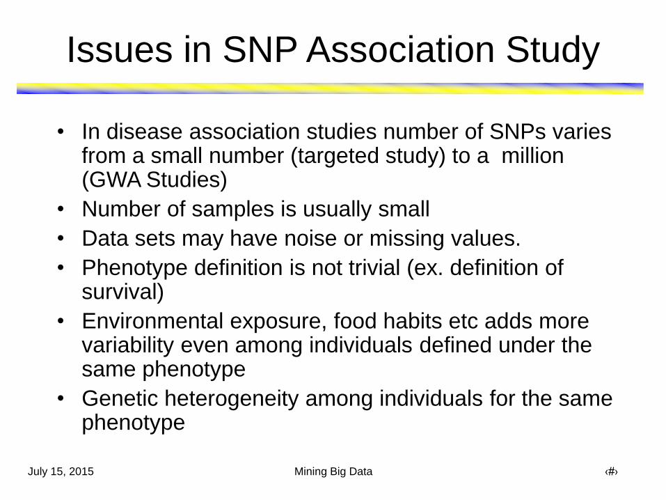
Issues in SNP Association Study
• In disease association studies number of SNPs varies from a small number (targeted study) to a million (GWA Studies)
• Number of samples is usually small
• Data sets may have noise or missing values.
• Phenotype definition is not trivial (ex. definition of survival)
• Environmental exposure, food habits etc adds more variability even among individuals defined under the same phenotype
• Genetic heterogeneity among individuals for the same phenotype

July 15, 2015 Mining Big Data ‹#›
Existing Analysis Methods
• Univariate Analysis: single SNP tested against the
phenotype for correlaton and ranked.
– Feasible but doesn‟t capture the existing true combinations.
• Multivariate Analysis: groups of SNPs of size two or
more are tested for possible association with the
phenotype.
– Infeasible but captures any true combinations.
• These two approaches are used to identify
biomarkers.
• Some approaches employ classification methods like
SVMs to classify cases and controls.

July 15, 2015 Mining Big Data ‹#›
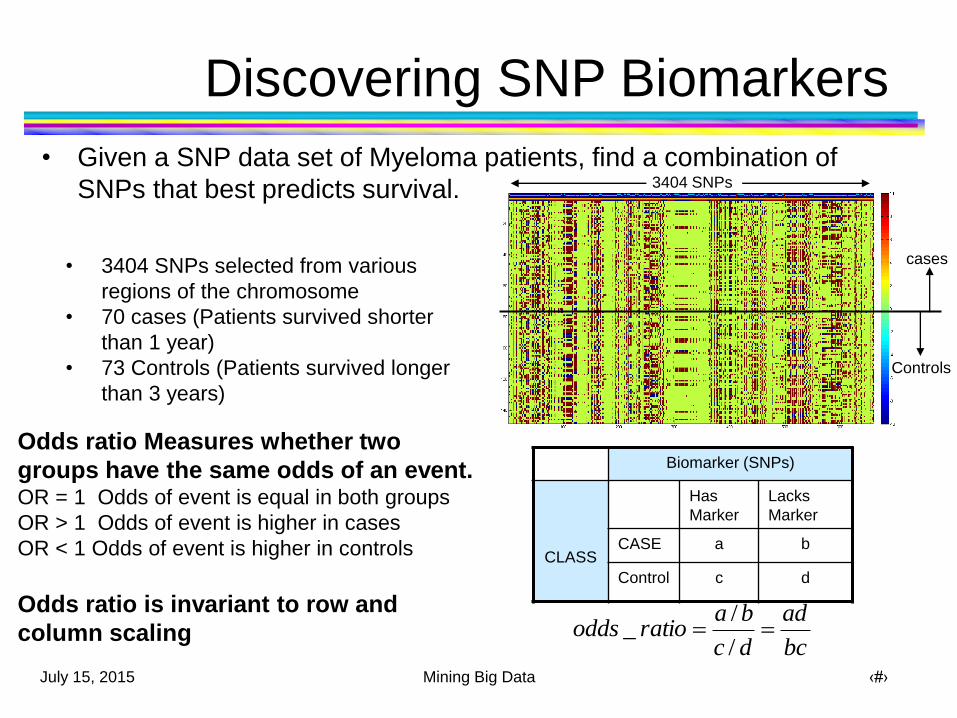
Discovering SNP Biomarkers
• Given a SNP data set of Myeloma patients, find a combination of
SNPs that best predicts survival.
• 3404 SNPs selected from various
regions of the chromosome
• 70 cases (Patients survived shorter
than 1 year)
• 73 Controls (Patients survived longer
than 3 years)
cases
Controls
3404 SNPs
Complexity of the Problem:
•Large number of SNPs (over a million in GWA studies) and small sample size
•Complex interaction among genes may be responsible for the phenotype
•Genetic heterogeneity among individuals sharing the same phenotype (due to environmental exposure, food habits, etc) adds more variability
•Complex phenotype definition (eg. survival)
July 15, 2015 Mining Big Data ‹#›
Discovering SNP Biomarkers
• Given a SNP data set of Myeloma patients, find a combination of
SNPs that best predicts survival.
• 3404 SNPs selected from various
regions of the chromosome
• 70 cases (Patients survived shorter
than 1 year)
• 73 Controls (Patients survived longer
than 3 years)
cases
Controls
3404 SNPs
Odds ratio Measures whether two
groups have the same odds of an event. OR = 1 Odds of event is equal in both groups
OR > 1 Odds of event is higher in cases
OR < 1 Odds of event is higher in controls
Odds ratio is invariant to row and
column scaling
Biomarker (SNPs)
CLASS
Has
Marker
Lacks
Marker
CASE a b
Control c d
bc
ad
dc
baratioodds
/
/_

July 15, 2015 Mining Big Data ‹#›
Discovering SNP Biomarkers
• Given a SNP data set of Myeloma patients, find a combination of
SNPs that best predicts survival.
• 3404 SNPs selected from various
regions of the chromosome
• 70 cases (Patients survived shorter
than 1 year)
• 73 Controls (Patients survived longer
than 3 years)
cases
Controls
3404 SNPs
Complexity of the Problem:
•Large number of SNPs (over a million in GWA studies) and small sample size
•Complex interaction among genes may be responsible for the phenotype
•Genetic heterogeneity among individuals sharing the same phenotype (due to environmental exposure, food habits, etc) adds more variability
•Complex phenotype definition (eg. survival)

July 15, 2015 Mining Big Data ‹#›
P-value
• P-value – Statistical terminology for a probability value
– Is the probability that the we get an odds ratio as extreme as the one we got by random chance
– Computed by using the chi-square statistic or Fisher‟s exact test
• Chi-square statistic is not valid if the number of entries in a cell of the contingency table is small
• p-value = 1 – hygecdf( a – 1, a+b+c+d, a+c, a+b ) if we are testing value is higher than expected by random chance using Fisher‟s exact test
• A statistical test to determine if there are nonrandom associations between two categorical variables.
– P-values are often expressed in terms of the negative log of p-value, e.g., -log10(0.005) = 2.3
53

July 15, 2015 Mining Big Data ‹#›
Discovering SNP Biomarkers
• Given a SNP data set of Myeloma patients, find a combination of
SNPs that best predicts survival.
• 3404 SNPs selected from various
regions of the chromosome
• 70 cases (Patients survived shorter
than 1 year)
• 73 Controls (Patients survived longer
than 3 years)
cases
Controls
3404 SNPs
Highest p-value,
moderate odds ratio
Highest odds ratio,
moderate p value
Moderate odds ratio,
moderate p value
July 15, 2015 Mining Big Data ‹#›
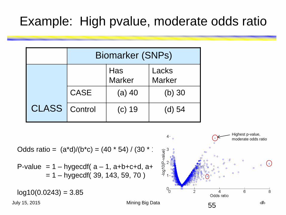
Example: High pvalue, moderate odds ratio
Biomarker (SNPs)
CLASS
Has
Marker
Lacks
Marker
CASE (a) 40 (b) 30
Control (c) 19 (d) 54
Odds ratio = (a*d)/(b*c) = (40 * 54) / (30 * 19) = 3.64
P-value = 1 – hygecdf( a – 1, a+b+c+d, a+c, a+b )
= 1 – hygecdf( 39, 143, 59, 70 )
log10(0.0243) = 3.85
55
Highest p-value,
moderate odds ratio

July 15, 2015 Mining Big Data ‹#›
Example …
Biomarker (SNPs)
CLASS
Has
Marker
Lacks
Marker
CASE (a) 7 (b) 63
Control (c) 1 (d) 72
Odds ratio = (a*d)/(b*c) = (7 * 72) / (63* 1) = 8
P-value = 1 – hygecdf( a – 1, a+b+c+d, a+c, a+b )
= 1 – hygecdf( 6, 143, 8, 70)
log10(pvalue) = 1.56
56
Highest odds ratio,
moderate p value
July 15, 2015 Mining Big Data ‹#›
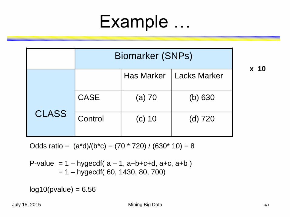
Example …
Biomarker (SNPs)
CLASS
Has Marker Lacks Marker
CASE (a) 70 (b) 630
Control (c) 10 (d) 720
Odds ratio = (a*d)/(b*c) = (70 * 720) / (630* 10) = 8
P-value = 1 – hygecdf( a – 1, a+b+c+d, a+c, a+b )
= 1 – hygecdf( 60, 1430, 80, 700)
log10(pvalue) = 6.56
x 10

July 15, 2015 Mining Big Data ‹#›
Example …
Biomarker (SNPs)
CLASS
Has Marker Lacks Marker
CASE (a) 140 (b) 1260
Control (c) 20 (d) 1440
Odds ratio = (a*d)/(b*c) = (140 * 1440) / (1260* 20) = 8
P-value = 1 – hygecdf( a – 1, a+b+c+d, a+c, a+b )
= 1 – hygecdf( 139, 2860, 160, 1400)
log10(pvalue) = 11.9
x 20

July 15, 2015 Mining Big Data ‹#›
Issues with Traditional Methods
Top ranked SNP:
-log10P-value = 3.8; Odds
Ratio = 3.7
• Each SNP is tested and
ranked individually
• Individual SNP
associations with true
phenotype are not
distinguishable from
random permutation of
phenotype
However, most reported associations are not robust: of the 166 putative
associations which have been studied three or more times, only 6 have
been consistently replicated.
Van Ness et al 2009

July 15, 2015 Mining Big Data ‹#›
Evaluating the Utility of Univariate Rankings
for Myeloma Data
Feature
Selection
Leave-one-out
Cross validation
With SVM
Biased Evaluation

July 15, 2015 Mining Big Data ‹#›
Evaluating the Utility of Univariate Rankings
for Myeloma Data
Feature
Selection
Leave-one-out
Cross validation
With SVM
Leave-one-out Cross
validation with SVM
Feature Selection
Biased Evaluation Clean Evaluation

July 15, 2015 Mining Big Data ‹#›
Random Permutation test
• Accuracy larger than 65% are highly significant. (p-value is < 10-4)
• 10,000 random permutations of real phenotype generated.
• For each one, Leave-one-out cross validation using SVM.

July 15, 2015 Mining Big Data ‹#›
Nearest Neighbor Classifier

July 15, 2015 Mining Big Data ‹#›
Nearest Neighbor Classifiers
• Basic idea:
– If it walks like a duck, quacks like a duck, then
it‟s probably a duck
Training
Records
Test
Record
Compute
Distance
Choose k of the
“nearest” records

July 15, 2015 Mining Big Data ‹#›
Nearest-Neighbor Classifiers
Requires three things
– The set of stored records
– Distance metric to compute
distance between records
– The value of k, the number of
nearest neighbors to retrieve
To classify an unknown record:
– Compute distance to other
training records
– Identify k nearest neighbors
– Use class labels of nearest
neighbors to determine the
class label of unknown record
(e.g., by taking majority vote)
Unknown record

July 15, 2015 Mining Big Data ‹#›
Nearest Neighbor Classification…
• Choosing the value of k: – If k is too small, sensitive to noise points
– If k is too large, neighborhood may include points
from other classes
X

July 15, 2015 Mining Big Data ‹#›
Clustering

July 15, 2015 Mining Big Data ‹#›
Clustering
• Finding groups of objects such that the objects in a
group will be similar (or related) to one another and
different from (or unrelated to) the objects in other
groups
Inter-cluster distances are maximized
Intra-cluster distances are
minimized
July 15, 2015 Mining Big Data ‹#›
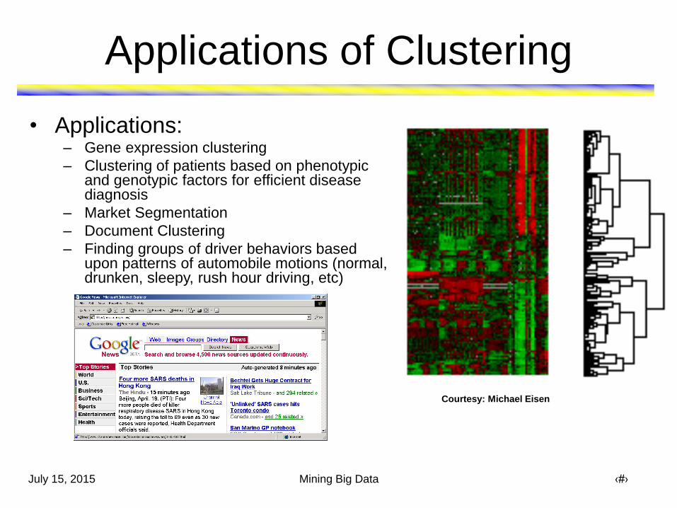
Applications of Clustering
• Applications: – Gene expression clustering
– Clustering of patients based on phenotypic and genotypic factors for efficient disease diagnosis
– Market Segmentation
– Document Clustering
– Finding groups of driver behaviors based upon patterns of automobile motions (normal, drunken, sleepy, rush hour driving, etc)
Courtesy: Michael Eisen
July 15, 2015 Mining Big Data ‹#›
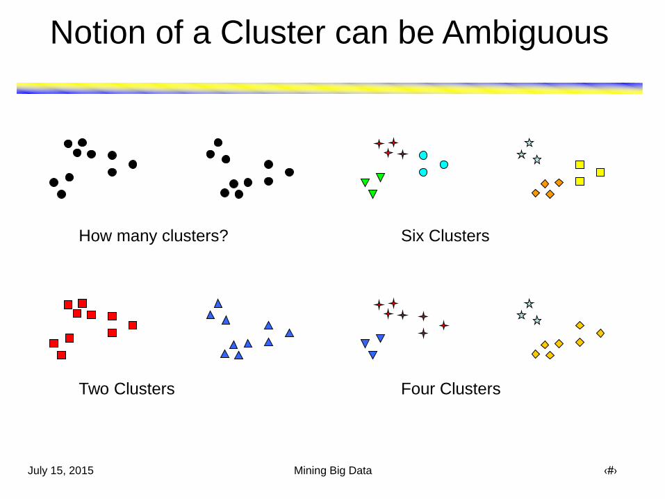
Notion of a Cluster can be Ambiguous
How many clusters?
Four Clusters Two Clusters
Six Clusters

July 15, 2015 Mining Big Data ‹#›
Similarity and Dissimilarity Measures
• Similarity measure
– Numerical measure of how alike two data objects are.
– Is higher when objects are more alike.
– Often falls in the range [0,1]
• Dissimilarity measure
– Numerical measure of how different are two data
objects
– Lower when objects are more alike
– Minimum dissimilarity is often 0
– Upper limit varies
• Proximity refers to a similarity or dissimilarity

July 15, 2015 Mining Big Data ‹#›
Euclidean Distance
• Euclidean Distance
Where n is the number of dimensions (attributes) and xk and yk
are, respectively, the kth attributes (components) or data objects x and y.
• Correlation
n
k
kk yxyxdist1
2)(),(
)()(
),cov(
)()(
))((
),(
1
2
1
2
1
2
ystdxstd
yx
yyxx
yyxx
yxcorrn
k
k
n
k
k
n
k
kk

July 15, 2015 Mining Big Data ‹#›
Types of Clusterings
• A clustering is a set of clusters
• Important distinction between hierarchical and partitional sets of clusters
• Partitional Clustering – A division data objects into
non-overlapping subsets (clusters) such that each data object is in exactly one subset
• Hierarchical clustering – A set of nested clusters organized
as a hierarchical tree p4p1 p2 p3
July 15, 2015 Mining Big Data ‹#›
Other Distinctions Between Sets of Clusters
• Exclusive versus non-exclusive – In non-exclusive clusterings, points may belong to multiple
clusters.
– Can represent multiple classes or „border‟ points
• Fuzzy versus non-fuzzy – In fuzzy clustering, a point belongs to every cluster with some
weight between 0 and 1
– Weights must sum to 1
– Probabilistic clustering has similar characteristics
• Partial versus complete – In some cases, we only want to cluster some of the data
• Heterogeneous versus homogeneous – Clusters of widely different sizes, shapes, and densities

July 15, 2015 Mining Big Data ‹#›
Clustering Algorithms
• K-means and its variants
• Hierarchical clustering
• Other types of clustering

July 15, 2015 Mining Big Data ‹#›
K-means Clustering
• Partitional clustering approach
• Number of clusters, K, must be specified
• Each cluster is associated with a centroid (center point)
• Each point is assigned to the cluster with the closest centroid
• The basic algorithm is very simple

Example of K-means Clustering
-2 -1.5 -1 -0.5 0 0.5 1 1.5 2
0
0.5
1
1.5
2
2.5
3
x
yIteration 1
-2 -1.5 -1 -0.5 0 0.5 1 1.5 2
0
0.5
1
1.5
2
2.5
3
x
yIteration 2
-2 -1.5 -1 -0.5 0 0.5 1 1.5 2
0
0.5
1
1.5
2
2.5
3
x
yIteration 3
-2 -1.5 -1 -0.5 0 0.5 1 1.5 2
0
0.5
1
1.5
2
2.5
3
x
yIteration 4
-2 -1.5 -1 -0.5 0 0.5 1 1.5 2
0
0.5
1
1.5
2
2.5
3
x
yIteration 5
-2 -1.5 -1 -0.5 0 0.5 1 1.5 2
0
0.5
1
1.5
2
2.5
3
x
yIteration 6

July 15, 2015 Mining Big Data ‹#›
K-means Clustering – Details
• The centroid is (typically) the mean of the points in
the cluster
• Initial centroids are often chosen randomly
– Clusters produced vary from one run to another
• „Closeness‟ is measured by Euclidean distance,
cosine similarity, correlation, etc
• Complexity is O( n * K * I * d )
– n = number of points, K = number of clusters,
I = number of iterations, d = number of attributes

July 15, 2015 Mining Big Data ‹#›
Evaluating K-means Clusters
• Most common measure is Sum of Squared Error (SSE)
– For each point, the error is the distance to the nearest cluster
– To get SSE, we square these errors and sum them
• x is a data point in cluster Ci and mi is the representative point for cluster Ci
– Given two sets of clusters, we prefer the one with the smallest error
– One easy way to reduce SSE is to increase K, the number of clusters
K
i Cx
i
i
xmdistSSE1
2 ),(

July 15, 2015 Mining Big Data ‹#›
Two different K-means Clusterings
-2 -1.5 -1 -0.5 0 0.5 1 1.5 2
0
0.5
1
1.5
2
2.5
3
x
y
-2 -1.5 -1 -0.5 0 0.5 1 1.5 2
0
0.5
1
1.5
2
2.5
3
x
y
Sub-optimal Clustering
-2 -1.5 -1 -0.5 0 0.5 1 1.5 2
0
0.5
1
1.5
2
2.5
3
x
y
Optimal Clustering
Original Points

July 15, 2015 Mining Big Data ‹#›
Limitations of K-means
• K-means has problems when clusters are
of differing
– Sizes
– Densities
– Non-globular shapes
• K-means has problems when the data
contains outliers.

July 15, 2015 Mining Big Data ‹#›
Limitations of K-means: Differing Sizes
Original Points K-means (3 Clusters)
July 15, 2015 Mining Big Data ‹#›
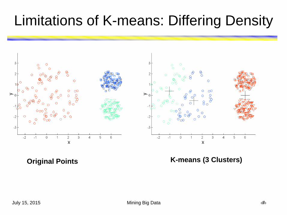
Limitations of K-means: Differing Density
Original Points K-means (3 Clusters)
July 15, 2015 Mining Big Data ‹#›
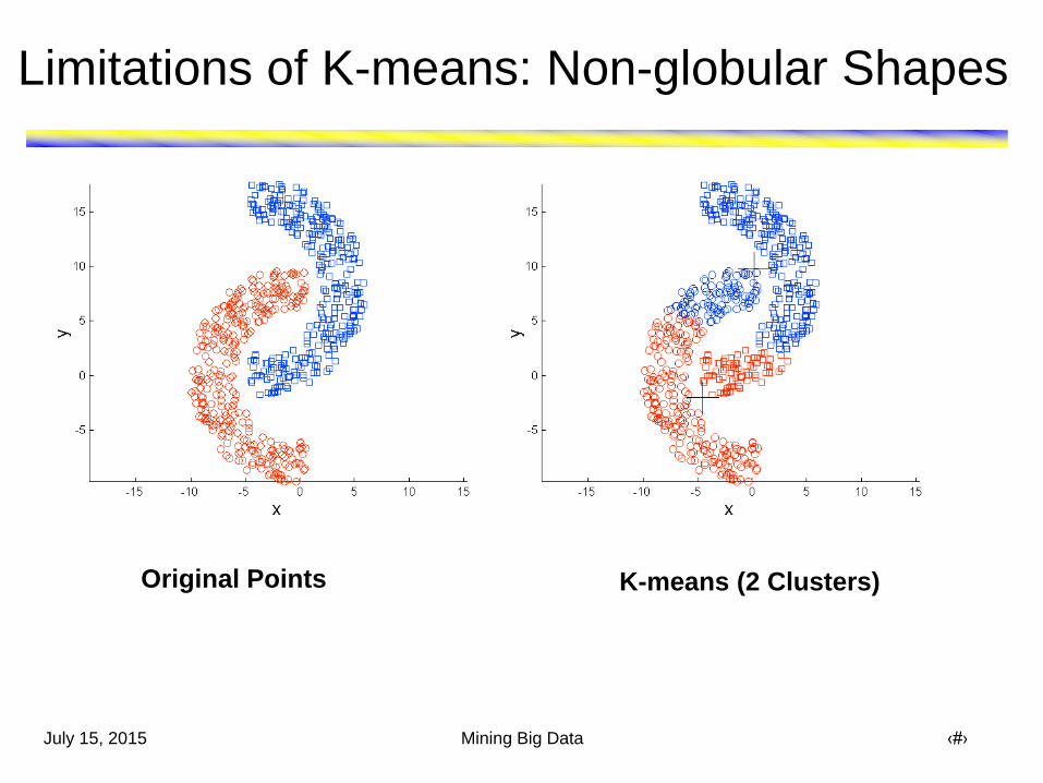
Limitations of K-means: Non-globular Shapes
Original Points K-means (2 Clusters)

July 15, 2015 Mining Big Data ‹#›
Hierarchical Clustering
• Produces a set of nested clusters
organized as a hierarchical tree
• Can be visualized as a
dendrogram
– A tree like diagram that records the
sequences of merges or splits
1
2
3
4
5
6
1
2
3
4
5
3 6 2 5 4 10
0.05
0.1
0.15
0.2

July 15, 2015 Mining Big Data ‹#›
Strengths of Hierarchical Clustering
• Do not have to assume any particular number of clusters – Any desired number of clusters can be obtained by
„cutting‟ the dendrogram at the proper level
• They may correspond to meaningful taxonomies – Example in biological sciences (e.g., animal kingdom,
phylogeny reconstruction, …)

July 15, 2015 Mining Big Data ‹#›
Hierarchical Clustering
• Two main types of hierarchical clustering
– Agglomerative: • Start with the points as individual clusters
• At each step, merge the closest pair of clusters until only one cluster (or k clusters) left
– Divisive: • Start with one, all-inclusive cluster
• At each step, split a cluster until each cluster contains a point (or there are k clusters)
• Traditional hierarchical algorithms use a similarity or distance matrix
– Merge or split one cluster at a time

July 15, 2015 Mining Big Data ‹#›
Agglomerative Clustering Algorithm
• More popular hierarchical clustering technique
• Basic algorithm is straightforward 1. Compute the proximity matrix
2. Let each data point be a cluster
3. Repeat
4. Merge the two closest clusters
5. Update the proximity matrix
6. Until only a single cluster remains
• Key operation is the computation of the proximity of two clusters
– Different approaches to defining the distance between clusters distinguish the different algorithms

July 15, 2015 Mining Big Data ‹#›
Starting Situation
• Start with clusters of individual points and
a proximity matrix
p1
p3
p5
p4
p2
p1 p2 p3 p4 p5 . . .
.
.
. Proximity Matrix
...p1 p2 p3 p4 p9 p10 p11 p12

July 15, 2015 Mining Big Data ‹#›
Intermediate Situation
• After some merging steps, we have some clusters
C1
C4
C2 C5
C3
C2 C1
C1
C3
C5
C4
C2
C3 C4 C5
Proximity Matrix
...p1 p2 p3 p4 p9 p10 p11 p12

July 15, 2015 Mining Big Data ‹#›
Intermediate Situation
• We want to merge the two closest clusters (C2 and
C5) and update the proximity matrix.
C1
C4
C2 C5
C3
C2 C1
C1
C3
C5
C4
C2
C3 C4 C5
Proximity Matrix
...p1 p2 p3 p4 p9 p10 p11 p12

July 15, 2015 Mining Big Data ‹#›
After Merging
• The question is “How do we update the proximity
matrix?”
C1
C4
C2 U C5
C3 ? ? ? ?
?
?
?
C2
U
C5 C1
C1
C3
C4
C2 U C5
C3 C4
Proximity Matrix
...p1 p2 p3 p4 p9 p10 p11 p12
July 15, 2015 Mining Big Data ‹#›
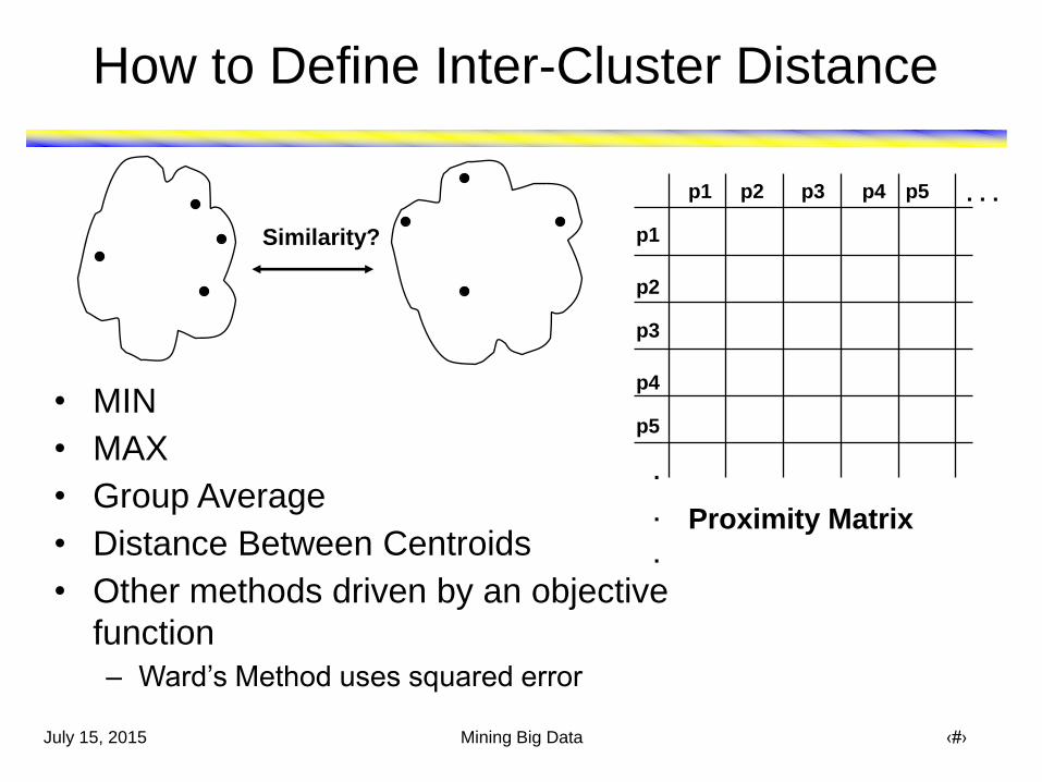
How to Define Inter-Cluster Distance
p1
p3
p5
p4
p2
p1 p2 p3 p4 p5 . . .
.
.
.
Similarity?
• MIN
• MAX
• Group Average
• Distance Between Centroids
• Other methods driven by an objective
function
– Ward‟s Method uses squared error
Proximity Matrix

July 15, 2015 Mining Big Data ‹#›
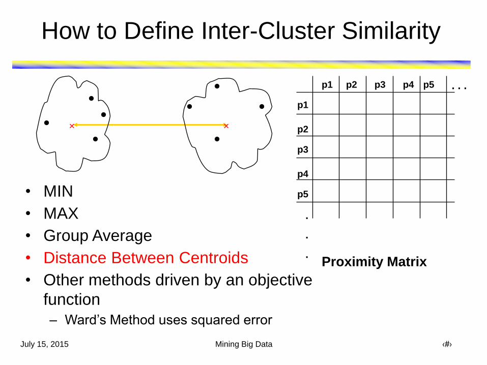
How to Define Inter-Cluster Similarity
p1
p3
p5
p4
p2
p1 p2 p3 p4 p5 . . .
.
.
. Proximity Matrix
• MIN
• MAX
• Group Average
• Distance Between Centroids
• Other methods driven by an objective
function
– Ward‟s Method uses squared error

July 15, 2015 Mining Big Data ‹#›
How to Define Inter-Cluster Similarity
p1
p3
p5
p4
p2
p1 p2 p3 p4 p5 . . .
.
.
. Proximity Matrix
• MIN
• MAX
• Group Average
• Distance Between Centroids
• Other methods driven by an objective
function
– Ward‟s Method uses squared error

July 15, 2015 Mining Big Data ‹#›
How to Define Inter-Cluster Similarity
p1
p3
p5
p4
p2
p1 p2 p3 p4 p5 . . .
.
.
. Proximity Matrix
• MIN
• MAX
• Group Average
• Distance Between Centroids
• Other methods driven by an objective
function
– Ward‟s Method uses squared error
July 15, 2015 Mining Big Data ‹#›
How to Define Inter-Cluster Similarity
p1
p3
p5
p4
p2
p1 p2 p3 p4 p5 . . .
.
.
. Proximity Matrix
• MIN
• MAX
• Group Average
• Distance Between Centroids
• Other methods driven by an objective
function
– Ward‟s Method uses squared error

July 15, 2015 Mining Big Data ‹#›
Other Types of Cluster Algorithms
• Hundreds of clustering algorithms
• Some clustering algorithms – K-means
– Hierarchical
– Statistically based clustering algorithms • Mixture model based clustering
– Fuzzy clustering
– Self-organizing Maps (SOM)
– Density-based (DBSCAN)
• Proper choice of algorithms depends on the type of clusters to be found, the type of data, and the objective

July 15, 2015 Mining Big Data ‹#›
Cluster Validity
• For supervised classification we have a variety of measures to evaluate how good our model is – Accuracy, precision, recall
• For cluster analysis, the analogous question is how to evaluate the “goodness” of the resulting clusters?
• But “clusters are in the eye of the beholder”!
• Then why do we want to evaluate them? – To avoid finding patterns in noise
– To compare clustering algorithms
– To compare two sets of clusters
– To compare two clusters

July 15, 2015 Mining Big Data ‹#›
Clusters found in Random Data
0 0.2 0.4 0.6 0.8 10
0.1
0.2
0.3
0.4
0.5
0.6
0.7
0.8
0.9
1
x
y
Random
Points
0 0.2 0.4 0.6 0.8 10
0.1
0.2
0.3
0.4
0.5
0.6
0.7
0.8
0.9
1
x
y
K-means
0 0.2 0.4 0.6 0.8 10
0.1
0.2
0.3
0.4
0.5
0.6
0.7
0.8
0.9
1
x
y
DBSCAN
0 0.2 0.4 0.6 0.8 10
0.1
0.2
0.3
0.4
0.5
0.6
0.7
0.8
0.9
1
x
y
Complete
Link

July 15, 2015 Mining Big Data ‹#›
• Distinguishing whether non-random structure actually exists in the
data
• Comparing the results of a cluster analysis to externally known
results, e.g., to externally given class labels
• Evaluating how well the results of a cluster analysis fit the data
without reference to external information
• Comparing the results of two different sets of cluster analyses to
determine which is better
• Determining the „correct‟ number of clusters
Different Aspects of Cluster Validation

July 15, 2015 Mining Big Data ‹#›
• Order the similarity matrix with respect to
cluster labels and inspect visually.
Using Similarity Matrix for Cluster Validation
0 0.2 0.4 0.6 0.8 10
0.1
0.2
0.3
0.4
0.5
0.6
0.7
0.8
0.9
1
x
y
Points
Po
ints
20 40 60 80 100
10
20
30
40
50
60
70
80
90
100Similarity
0
0.1
0.2
0.3
0.4
0.5
0.6
0.7
0.8
0.9
1

July 15, 2015 Mining Big Data ‹#›
Using Similarity Matrix for Cluster Validation
• Clusters in random data are not so crisp
Points
Po
ints
20 40 60 80 100
10
20
30
40
50
60
70
80
90
100Similarity
0
0.1
0.2
0.3
0.4
0.5
0.6
0.7
0.8
0.9
1
DBSCAN
0 0.2 0.4 0.6 0.8 10
0.1
0.2
0.3
0.4
0.5
0.6
0.7
0.8
0.9
1
x
y

July 15, 2015 Mining Big Data ‹#›
Points
Po
ints
20 40 60 80 100
10
20
30
40
50
60
70
80
90
100Similarity
0
0.1
0.2
0.3
0.4
0.5
0.6
0.7
0.8
0.9
1
Using Similarity Matrix for Cluster Validation
• Clusters in random data are not so crisp
K-means
0 0.2 0.4 0.6 0.8 10
0.1
0.2
0.3
0.4
0.5
0.6
0.7
0.8
0.9
1
x
y

July 15, 2015 Mining Big Data ‹#›
Using Similarity Matrix for Cluster Validation
• Clusters in random data are not so crisp
0 0.2 0.4 0.6 0.8 10
0.1
0.2
0.3
0.4
0.5
0.6
0.7
0.8
0.9
1
x
y
Points
Po
ints
20 40 60 80 100
10
20
30
40
50
60
70
80
90
100Similarity
0
0.1
0.2
0.3
0.4
0.5
0.6
0.7
0.8
0.9
1
Complete Link
July 15, 2015 Mining Big Data ‹#›
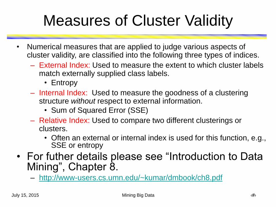
• Numerical measures that are applied to judge various aspects of cluster validity, are classified into the following three types of indices.
– External Index: Used to measure the extent to which cluster labels match externally supplied class labels.
• Entropy
– Internal Index: Used to measure the goodness of a clustering structure without respect to external information.
• Sum of Squared Error (SSE)
– Relative Index: Used to compare two different clusterings or clusters.
• Often an external or internal index is used for this function, e.g., SSE or entropy
• For futher details please see “Introduction to Data Mining”, Chapter 8. – http://www-users.cs.umn.edu/~kumar/dmbook/ch8.pdf
Measures of Cluster Validity

July 15, 2015 Mining Big Data ‹#›
Clustering Microarray Data

July 15, 2015 Mining Big Data ‹#›
Clustering Microarray Data
• Microarray analysis allows the monitoring of the
activities of many genes over many different
conditions
• Data: Expression profiles of approximately 3606
genes of E Coli are recorded for 30 experimental
conditions
• SAM (Significance Analysis of Microarrays) package
from Stanford University is used for the analysis of
the data and to identify the genes that are
substantially differentially upregulated in the dataset –
17 such genes are identified for study purposes
• Hierarchical clustering is performed and plotted using
TreeView
Gene1
Gene2
Gene3
Gene4
Gene5
Gene6
Gene7
….
C1 C2 C3 C4 C5 C6 C7

July 15, 2015 Mining Big Data ‹#›
Clustering Microarray Data…

July 15, 2015 Mining Big Data ‹#›
CLUTO for Clustering for Microarray Data
• CLUTO (Clustering Toolkit) George Karypis (UofM)
http://glaros.dtc.umn.edu/gkhome/views/cluto/
• CLUTO can also be used for clustering microarray data

July 15, 2015 Mining Big Data ‹#›
Issues in Clustering Expression Data
• Similarity uses all the conditions
– We are typically interested in sets of genes that are
similar for a relatively small set of conditions
• Most clustering approaches assume that an
object can only be in one cluster
– A gene may belong to more than one functional group
– Thus, overlapping groups are needed
• Can either use clustering that takes these
factors into account or use other techniques
– For example, association analysis
July 15, 2015 Mining Big Data ‹#›
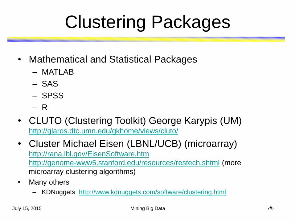
Clustering Packages
• Mathematical and Statistical Packages
– MATLAB
– SAS
– SPSS
– R
• CLUTO (Clustering Toolkit) George Karypis (UM) http://glaros.dtc.umn.edu/gkhome/views/cluto/
• Cluster Michael Eisen (LBNL/UCB) (microarray) http://rana.lbl.gov/EisenSoftware.htm
http://genome-www5.stanford.edu/resources/restech.shtml (more
microarray clustering algorithms)
• Many others
– KDNuggets http://www.kdnuggets.com/software/clustering.html

July 15, 2015 Mining Big Data ‹#›
Association Analysis

July 15, 2015 Mining Big Data ‹#›
Association Analysis
• Given a set of records, find dependency rules which will predict occurrence of an item based on occurrences of other items in the record
• Applications
– Marketing and Sales Promotion
– Supermarket shelf management
– Traffic pattern analysis (e.g., rules such as "high congestion on Intersection 58 implies high accident rates for left turning traffic")
TID Items
1 Bread, Coke, Milk
2 Beer, Bread
3 Beer, Coke, Diaper, Milk
4 Beer, Bread, Diaper, Milk
5 Coke, Diaper, Milk
Rules Discovered:
{Milk} --> {Coke} (s=0.6, c=0.75)
{Diaper, Milk} --> {Beer} (s=0.4, c=0.67)
ons transactiTotal
Y and Xcontain that ons transacti# s Support,
Xcontain that ons transacti#
Y and Xcontain that ons transacti# c ,Confidence

July 15, 2015 Mining Big Data ‹#›
Association Rule Mining Task
• Given a set of transactions T, the goal of association
rule mining is to find all rules having – support ≥ minsup threshold
– confidence ≥ minconf threshold
• Brute-force approach: Two Steps – Frequent Itemset Generation
• Generate all itemsets whose support minsup
– Rule Generation
• Generate high confidence rules from each frequent itemset, where each rule is a binary partitioning of a frequent itemset
• Frequent itemset generation is computationally expensive

July 15, 2015 Mining Big Data ‹#›
Efficient Pruning Strategy (Ref: Agrawal & Srikant
1994)
If an itemset is infrequent,
then all of its supersets
must also be infrequent
null
AB AC AD AE BC BD BE CD CE DE
A B C D E
ABC ABD ABE ACD ACE ADE BCD BCE BDE CDE
ABCD ABCE ABDE ACDE BCDE
ABCDE
Found to be
Infrequent
null
AB AC AD AE BC BD BE CD CE DE
A B C D E
ABC ABD ABE ACD ACE ADE BCD BCE BDE CDE
ABCD ABCE ABDE ACDE BCDE
ABCDE
null
AB AC AD AE BC BD BE CD CE DE
A B C D E
ABC ABD ABE ACD ACE ADE BCD BCE BDE CDE
ABCD ABCE ABDE ACDE BCDE
ABCDE
Pruned
supersets

July 15, 2015 Mining Big Data ‹#›
Illustrating Apriori Principle
Item Count
Bread 4Coke 2Milk 4Beer 3Diaper 4Eggs 1
Itemset Count
{Bread,Milk} 3{Bread,Beer} 2{Bread,Diaper} 3{Milk,Beer} 2{Milk,Diaper} 3{Beer,Diaper} 3
Itemset Count
{Bread,Milk,Diaper} 3
Items (1-itemsets)
Pairs (2-itemsets) (No need to generate candidates involving Coke or Eggs)
Triplets (3-itemsets) Minimum Support = 3
If every subset is considered, 6C1 + 6C2 + 6C3 = 41 With support-based pruning, 6 + 6 + 1 = 13

July 15, 2015 Mining Big Data ‹#›
Association Measures
• Association measures evaluate the strength of an association pattern – Support and confidence are the most commonly used
– The support, (X), of an itemset X is the number of transactions that contain all the items of the itemset
• Frequent itemsets have support > specified threshold
• Different types of itemset patterns are distinguished by a
measure and a threshold
– The confidence of an association rule is given by conf(X Y) = (X Y) / (X)
• Estimate of the conditional probability of Y given X
• Other measures can be more useful – H-confidence
– Interest

July 15, 2015 Mining Big Data ‹#›
Application on Biomedical Data

July 15, 2015 Mining Big Data ‹#›
• Differential expression Differential coexpression
• Differential Expression (DE)
– Traditional analysis targets the changes of expression level
Expression over samples in controls and cases
Exp
ressio
n l
evel
controls cases
[Golub et al., 1999], [Pan 2002], [Cui and Churchill, 2003] etc.
Mining Differential Coexpression (DC)

July 15, 2015 Mining Big Data ‹#›
Matrix of expression values
• Differential Coexpression (DC)
– Targets changes of the coherence of expression
controls cases Question: Is this gene interesting,
i.e. associated w/ the phenotype?
Answer: No, in term of differential
expression (DE).
However, what if there are
another two genes ……?
Yes! Expression over samples
in controls and cases
Differential Coexpression (DC)
[Silva et al., 1995], [Li, 2002], [Kostka & Spang, 2005], [Rosemary et al., 2008], [Cho et al. 2009] etc.
Biological interpretations of DC:
Dysregulation of pathways, mutation of transcriptional factors, etc.
genes
controls cases
[Kostka & Spang, 2005]

July 15, 2015 Mining Big Data ‹#›
• Existing work on differential coexpression – Pairs of genes with differential coexpression
• [Silva et al., 1995], [Li, 2002], [Li et al., 2003], [Lai et al. 2004]
– Clustering based differential coexpression analysis • [Ihmels et al., 2005], [Watson., 2006]
– Network based analysis of differential coexpression • [Zhang and Horvath, 2005], [Choi et al., 2005], [Gargalovic et al. 2006],
[Oldham et al. 2006], [Fuller et al., 2007], [Xu et al., 2008]
– Beyond pair-wise (size-k) differential coexpression • [Kostka and Spang., 2004], [Prieto et al., 2006]
– Gene-pathway differential coexpression • [Rosemary et al., 2008]
– Pathway-pathway differential coexpression • [Cho et al., 2009]
Differential Coexpression (DC)

July 15, 2015 Mining Big Data ‹#›
• Full-space differential coexpression
• May have limitations due to the heterogeneity of – Causes of a disease (e.g. genetic difference)
– Populations affected (e.g. demographic difference)
Existing DC work is “full-space”
Motivation:
Such subspace patterns
may be missed by full-
space models
Full-space measures: e.g.
correlation difference

July 15, 2015 Mining Big Data ‹#›
• Definition of Subspace Differential Coexpression Pattern – A set of k genes = {g1, g2 ,…, gk}
– : Fraction of samples in class A, on which the k genes are coexpressed
– : Fraction of samples in class B, on which the k genes are coexpressed
Extension to Subspace Differential Coexpression
Details in [Fang, Kuang, Pandey, Steinbach, Myers and Kumar, PSB 2010]
as a measure of subspace differential coexpression
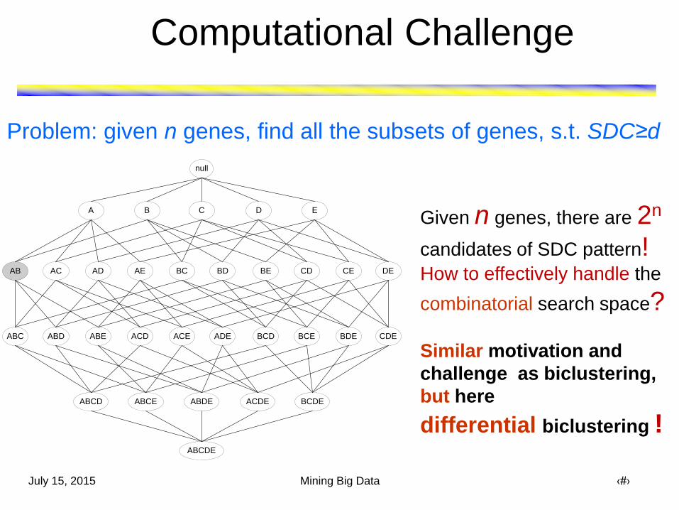
Problem: given n
genes, find all the
subsets of genes,
s.t. SDC≥d
July 15, 2015 Mining Big Data ‹#›
Computational Challenge
Given n genes, there are 2n
candidates of SDC pattern! How to effectively handle the
combinatorial search space?
Similar motivation and
challenge as biclustering,
but here
differential biclustering !
null
AB AC AD AE BC BD BE CD CE DE
A B C D E
ABC ABD ABE ACD ACE ADE BCD BCE BDE CDE
ABCD ABCE ABDE ACDE BCDE
ABCDE
Problem: given n genes, find all the subsets of genes, s.t. SDC≥d

July 15, 2015 Mining Big Data ‹#›
Direct Mining of Differential Patterns
[Fang, Pandey, Gupta, Steinbach and Kumar, IEEE TKDE 2011]
Refined SDC measure: “direct”
A measure M is antimonotonic
if V A,B: A B M(A) >= M(B)
Details in [Fang, Kuang, Pandey, Steinbach, Myers and Kumar, PSB 2010]
>>
≈

July 15, 2015 Mining Big Data ‹#›
Advantages:
1) Systematic & direct
2) Completeness
3) Efficiency
null
AB AC AD AE BC BD BE CD CE DE
A B C D E
ABC ABD ABE ACD ACE ADE BCD BCE BDE CDE
ABCD ABCE ABDE ACDE BCDE
ABCDE
An Association-analysis Approach
[ Agrawal et al. 1994]
null
AB AC AD AE BC BD BE CD CE DE
A B C D E
ABC ABD ABE ACD ACE ADE BCD BCE BDE CDE
ABCD ABCE ABDE ACDE BCDE
ABCDE
Refined SDC measure
A measure M is antimonotonic if
V A,B: A B M(A) >= M(B)
Disqualified
Prune all the
supersets

July 15, 2015 Mining Big Data ‹#›
A 10-gene Subspace DC Pattern
www. ingenuity.com: enriched Ingenuity subnetwork
≈ 60% ≈ 10%
Enriched with the TNF-α/NFkB signaling pathway
(6/10 overlap with the pathway, P-value: 1.4*10-5)
Suggests that the dysregulation of TNF-α/NFkB
pathway may be related to lung cancer

July 15, 2015 Mining Big Data ‹#›
Data Mining Book
For further details and sample
chapters see
www.cs.umn.edu/~kumar/dmbook

July 15, 2015 Mining Big Data ‹#›
References
• Book
• Computational Approaches for Protein Function Prediction, Gaurav Pandey, Vipin Kumar and Michael Steinbach, to be published by John Wiley and Sons in the Book Series on Bioinformatics in Fall 2007
• Conferences/Workshops
• Association Analysis-based Transformations for Protein Interaction Networks: A Function Prediction Case Study, Gaurav Pandey, Michael Steinbach, Rohit Gupta, Tushar Garg and Vipin Kumar, to appear, ACM SIGKDD 2007
• Incorporating Functional Inter-relationships into Algorithms for Protein Function Prediction, Gaurav Pandey and Vipin Kumar, to appear, ISMB satellite meeting on Automated Function Prediction 2007
• Comparative Study of Various Genomic Data Sets for Protein Function Prediction and Enhancements Using Association Analysis, Rohit Gupta, Tushar Garg, Gaurav Pandey, Michael Steinbach and Vipin Kumar, To be published in the proceedings of the Workshop on Data Mining for Biomedical Informatics, held in conjunction with SIAM International Conference on Data Mining, 2007
• Identification of Functional Modules in Protein Complexes via Hyperclique Pattern Discovery, Hui Xiong, X. He, Chris Ding, Ya Zhang, Vipin Kumar and Stephen R. Holbrook, pp 221-232, Proc. of the Pacific Symposium on Biocomputing, 2005
• Feature Mining for Prediction of Degree of Liver Fibrosis, Benjamin Mayer, Huzefa Rangwala, Rohit Gupta, Jaideep Srivastava, George Karypis, Vipin Kumar and Piet de Groen, Proc. Annual Symposium of American Medical Informatics Association (AMIA), 2005
• Technical Reports
• Association Analysis-based Transformations for Protein Interaction Networks: A Function Prediction Case Study, Gaurav Pandey, Michael Steinbach, Rohit Gupta, Tushar Garg, Vipin Kumar, Technical Report 07-007, March 2007, Department of Computer Science, University of Minnesota
• Computational Approaches for Protein Function Prediction: A Survey, Gaurav Pandey, Vipin Kumar, Michael Steinbach, Technical Report 06-028, October 2006, Department of Computer Science, University of Minnesota