A Kinemati View of Loop ClosureEvangelos A. Coutsias1�, Chaok Seok2�,Matthew P. Ja obson2, and Ken A. Dill21Department of Mathemati s and Statisti s,University of New Mexi o,Albuquerque, New Mexi o 87131.2Department of Pharma euti al Chemistry,University of California in San Fran is o,San Fran is o, California 94107.Journal of Computational Chemistry (A epted 4 Nov. 2003)June 25, 2003A�� o ��o& o �� �& �!������Abstra tWe onsider the problem of loop losure, i.e., of �nding the ensem-ble of possible ba kbone stru tures of a hain segment of a proteinmole ule that is geometri ally onsistent with pre eding and followingparts of the hain whose stru tures are given. We redu e this problemof determining the loop onformations of six torsions to �nding thereal roots of a 16th degree polynomial in one variable, based on theroboti s literature on the kinemati s of the equivalent rotator linkagein the most general ase of oblique rotators. We provide a simpleintuitive view and derivation of the polynomial for the ase in whi hea h of the three pairs of torsional axes has a ommon point. Ourmethod generalizes previous work on analyti al loop losure in that�E. A. C. and C. S. ontributed equally to this study.1

the torsion angles need not be onse utive, and any rigid interveningsegments are allowed between the free torsions. Our approa h alsoallows for a small degree of exibility in the bond angles and the pep-tide torsion angles; this substantially enlarges the spa e of solvable on�gurations as is demonstrated by an appli ation of the method tothe modeling of y li pentapeptides. We give further appli ationsto two important problems. First, we show that this analyti al loop losure algorithm an be eÆ iently ombined with an existing loop- onstru tion algorithm to sample loops longer than three residues.Se ond, we show that Monte Carlo Minimization is made several-fold more eÆ ient by employing the lo al moves generated by theloop losure algorithm, when applied to the global minimization of aneight-residue loop. Our loop losure algorithm is freely available athttp://dillgroup.u sf.edu/loop_ losure/.1 Introdu tionWe onsider the problem of loop losure, i.e., �nding stru tures of a seg-ment in a hain mole ule that are geometri ally onsistent with the rest ofthe hain stru ture. This problem has an important appli ation in homol-ogy modeling [1℄, when segments of insertions or deletions are to be modeledwhile the rest of the protein stru ture is relatively well known from stru turesof homologous proteins. Another useful appli ation is in the area of MonteCarlo simulations, where alternative segment stru tures an be introdu edas elementary lo alized moves [2, 3, 4, 5, 6, 7, 8, 9, 10, 11℄. These moves an lead to improved eÆ ien y in onformational sampling. Unlike Carte-sian moves, they avoid geometri distortions and the high energy penaltythese entail. On the other hand, the deformation produ ed by these movesis limited to a segment, while un oordinated torsion angle moves result inmovement proportional to the distan e of ea h atom from the perturbationaxes, resulting in large un ontrolled moves. Other possible appli ations ofthe loop losure problem are dis ussed in Ref. [12℄.It is well known that the number of onstraints is identi al to the num-ber of degrees of freedom (DOFs) in the ase of loops with six free torsionangles, or three residue loops for proteins [13℄. This means that, in general,su h loops may be found as dis rete solutions of the loop losure problem.This fa t has been known for some time in the Kinemati theory of Me h-anisms [14℄. Kinemati s is the bran h of me hani s whose on ern is the2

geometri analysis of motion, espe ially onstrained displa ements withoutregard to for es. The kinemati analysis of systems of rigid obje ts onne tedby exible joints, su h as multi-jointed roboti manipulators, exhibits manysimilarities with the geometri analysis of ma romole ules, when the for esresponsible for the motions are ignored and the main question of interestis the analysis of possible onformations onsistent with the onstraints as-so iated with bond lengths and bond angles. In roboti s, joints that allowone arm to rotate about another at a �xed angle are alled Rotator pairsor \R-pairs". The arm system analogous to a ma romole ule with 6 rotat-able bonds is a \6R" linkage. The kinemati analysis of these and othersimilar linkages leads to Fourier polynomials in the six rotation angles, �i,i.e., polynomials in the variables os �i; sin �i. By introdu ing the half-angletransformationui = tan(�i=2) ! sin �i = 2ui1 + u2i ; os �i = 1� u2i1 + u2i ; i = 1; : : : ; 6;there results a system of polynomial equations in the ui. A polynomial for-mulation o�ers several advantages, su h as relative ease of solution, availabletheorems for the a urate enumeration of the number of solutions within agiven region when there is only a dis rete number, and in general better un-derstood numeri al properties. For instan e, the number of real roots of aunivariate polynomial equation ontained in an interval an be readily deter-mined by Sturm's method [15℄. No su h method is available for more general,trans endental equations. Therefore, an advantage of our polynomial equa-tion ompared to the trans endental equation of G�o and S heraga [13℄ is thatthe exa t number of solutions an be found, whi h is important for satisfyingmi ros opi reversibility in Monte Carlo simulations [3℄. Methods from alge-brai geometry [16, 17℄ and homotopy theory [18℄ have been applied to su hsystems, and robust algorithms exist for the determination of their solutions,real or omplex. A thorough dis ussion of roboti linkage systems an befound in the text by Du�y [19℄, while informative expositions and reviewsof the relevant literature an be found in the lassi text by Hartenberg andDenavit [14℄ and more re ently in the text by Hunt [20℄. A relatively urrentsurvey is given in Mano ha [21℄.The problem of losing 6R loops is entral for the ontrol of roboti manipulators, where in many ommon appli ations one end is �xed and theother (the \end e�e tor") must be positioned at a spe i� lo ation and witha given orientation. Adding a 7th rotator gives a system with one additional3

DOF, o�ering the possibility of ontinuous motion with two �xed ends. Thisproblem, hara terized as \The Mount Everest of roboti manipulators" byFreudenstein [22℄ was redu ed to a single variable, 16th degree polynomialequation by Lee and Liang [23℄. In their solution, the 7th rotational DOFis used as a ontrol parameter, and the real solutions obtained for the otherangles on e the 7th angle is �xed provide alternative losure on�gurations forthe system. The method applies to systems with arbitrary axes of rotation,but the derivation is quite involved and it is diÆ ult to arrive at an intuitiveunderstanding of its solutions and the implied hain displa ements.In this paper we onsider an important spe ial ase in whi h the 6Rproblem has an intuitively simple des ription: onsider all the motions of a hain mole ule that involve hanges in only six ba kbone torsions. If these arearranged so that they form three oterminal pairs, then the segments betweensu essive pairs will form e�e tively a oarser hain of 3 ( losed ase) or 4(open ase) rigid bodies, joined at the lo ations of the paired torsion axes.An illustration is given in Fig. 1 for a tri-peptide example, where the 4 rigidbodies are (N1 C�1), (C�1 C1 N2 C�2), (C�2 C2 N3 C�3), and (C�3 C3). Ifwe now require the two end segments of the hain (N1 C�1) and (C�3 C3)to remain at a �xed position relative to ea h other, (C�3 C3 N1 C�1) formsa third segment. Now ea h of the three rigid units (C�1 C1 N2 C�2), (C�2C2 N3 C�3), and (C�3 C3 N1 C�1) has two jun tions on it, atta hing to theother two units. De�ne the line onne ting the two jun tions on a unit asthe virtual axis of the unit (C�1{C�2, C�2{C�3, and C�3{C�1). The motionsof the middle two segments relative to the rest of the hain an only be omposed of individual rotations of ea h about their respe tive virtual axes(C�1{C�2 and C�2{C�3) or joint rotations of the two as a unit about the third(�xed) axis (C�3{C�1). The three virtual axes form a triangle, with verti esat the three jun tions (C�1, C�2, and C�3). If we rotate ea h of the unitsabout its axis by some angle �i; i = 1; 2; 3, the rotatable bonds at eitherend of the unit maintain a �xed dihedral with the axis and ea h other (adihedral formed by C�1{C1, C1{N2, and N2{C�2, for example). Any possiblemotion that a on erted hange in the original six torsions is apable of anthus be des ribed in terms of these three angles. If we now require that bondangles (�i) between the a tual bonds at the jun tion of two segments remainat a given value, these motions be ome oupled. The feasible on�gurationswhere all onstraints are satis�ed form a dis rete set, found as the solutionsof a polynomial equation in the orresponding three variables ui; i = 1; 2; 3.Having sets of rotation axes arranged in oterminal pairs is a natural property4

Figure 1: De�nition of three variables �1, �2, and �3 and three onstraints on�1, �2, and �3 in the anoni al tripeptide loop losure problem.5

of polypeptide hain ba kbones where one en ounters pairs of rotatable bondsat ea h C� atom (with the ex eption of proline), and similar pairings are ommon in other mole ules of interest, su h as RNA where groupings of 5pairwise oterminal rotatable bonds in the phosphate ba kbone are separatedby relatively rigid sugar rings.In its simplest form our algorithm may utilize the torsion angles at 3 C�atoms lo ated onse utively along a peptide ba kbone. This is the \tripep-tide loop losure" problem. The tripeptide loop losure problem was �rst onsidered by G�o and S heraga [13℄, who redu ed the problem to solving atrans endental equation in a single variable in the ase of planar peptide tor-sion angles. The method has found numerous appli ations and extensions.Bru oleri and Karplus [24℄ allowed small variation in bond angles as a meansof extending the method to over normal variability of these parameters inproteins of known stru tures, and applied the method to loop modeling [25℄.Dinner [7℄ produ ed a generalization to the non-planar peptide ase, still interms of trans endental equations. More re ently, Wedemeyer and S heraga[12℄ derived a single variable 16th degree polynomial equation for the par-ti ular ase of loop losure involving three onse utive residues with planarpeptide torsions at anoni al bond lengths and angles, i.e., when only three onse utive pairs of � and torsion angles are allowed to vary.One of the generalizations possible with our algorithm is for the threepairs of torsion angles with oterminal axes to be hosen along a mole u-lar hain with arbitrary, �xed stru ture between su essive pairs, in ludingnonplanar peptide torsion angles. This generalization is useful for severalreasons. Sampling with �xed bond angles and peptide torsion angles ansigni� antly limit the overage of onformational spa e [24℄, and moreover u tuations of order � 10o for the bond angles and peptide torsion anglesare not un ommon among proteins of known stru ture. Further, the methodpresented here allows for the torsion angles parti ipating in the move to be hosen at arbitrary lo ations along the hain. This allows its appli ationto diverse situations, su h as to the modeling of longer loops and loops inpolymers and nu lei a ids. Although it is possible to derive a des riptionin terms of a 16th degree polynomial even if all the angles are hosen om-pletely independently [26℄, the hoi e of paired �- angles leads to a simpleformulation in terms of three natural angle variables:� Choose three C� arbons lo ated su essively (but not ne essarily on-se utively) along the hain, say C�i; i = 1; 2; 3.6

� Rotate the segment C�1; : : : ; C�2 by angle �1 about the axis C�1{C�2.� Rotate the segment C�2; : : : ; C�3 by angle �2 about the axis C�2{C�3.� Rotate the segment C�1; : : : ; C�2; : : : ; C�3 by angle �3 about the axisC�1{C�3.� Choose the angles �i; i = 1; 2; 3 so that the bond angles Ni{C�i{C 0iassume (near) anoni al values at ea h of the atoms C�i.Satisfa tion of the ompatibility onditions in the last step is assured by thesolution of the polynomial system mentioned above, and every real solutionresults in a distin t on�guration. The analysis an easily be applied to hainsof arbitrary stru ture (i.e., it is not limited to polypeptides), provided thereexist pairs of o-terminal rotatable bonds. In the roboti s literature, R-jointswith axes that have a ommon point are referred as \spheri al pairs". We arethus studying the 6R system with three inter onne ted spheri al pairs [19℄.Problems of stru ture similar to the tripeptide loop losure problem are also ommon in another area of omputational geometry: the motion planningfor the assembly of four solid obje ts an be ast in identi al mathemati alform [27℄.Given that the general 6R problem an be des ribed by a 16th degreepolynomial, it follows that there will always be an even number of real so-lutions, ounting multipli ities, and at most 16 distin t real solutions arepossible, leading in turn to at most 16 distin t loop on�gurations. Su han example has been found by Manseur and Doty [28℄ for a 6R roboti ma-nipulator. Dodd et al. [3℄ in their study of on erted rotations in polymersystems report as many as 12 solutions in ertain ases, but sin e they studythe problem in its trans endental form they need to rely on expensive, ex-haustive sear hes to arrive at a omplete enumeration with on�den e. Forthe anoni al tripeptide loop losure, Wedemeyer and S heraga [12℄ havefound at most 8 real solutions of the losure polynomial and, hen e, at most8 distin t onformations. Our own studies with the more general peptide ge-ometry have so far only dis overed ases with at most 10 real solutions, andwe believe that this might be a limitation due to the fa t that the buildingblo ks of the problem are of spe ial form, perhaps not apable of overingthe entire set of possible behaviors of the polynomial system unless a ertainvariability in the parameters is introdu ed. For example, the obtuseness ofthe bond angles at the C� arbons should be ontrasted with the fa t that7

the angles between su essive arms of the manipulator in [28℄ are all �=2ex ept for one pair of parallel axes.Even though it is obvious that the analyti al loop losure method is ex-a t and mu h more eÆ ient ompared to numeri al loop losure methods[29, 30℄ for three residue loops, appli ation of the analyti al method to mod-eling longer loops has not yet been explored extensively. For loops of ntorsion angles, (n�6) DOFs need to be sampled with some additional sear hmethod. Here we employ an existing loop onstru tion method [31℄ to sample(n� 6) torsion angles, and solve for the remaining 6 torsion angles using an-alyti al loop losure. Other approa hes su h as a hierar hi al method and ade imation method have been suggested by Wedemeyer and S heraga [12℄ forsampling longer loops using an analyti al loop losure method. We sample(n�6) torsion angles dire tly be ause it is possible to in orporate s reeningsfor Rama handran allowed regions and steri lashes. These s reens enhan ethe eÆ ien y of sampling be ause they an be applied at early stages, andnon-promising stru tures an be pruned out before the whole model loop is onstru ted.We believe that an advantage of our work is the simpli�ed, intuitive viewof the tripeptide loop stru ture (or 6 free torsion angles in general), whi henables us to develop insights for useful appli ations. General theory andmethods are presented in Se tion 2, and results of appli ations in Se tion 3.In Se tion 2.1, we des ribe the simple view of the tripeptide loop losure,derive the loop losure equation, and present an eÆ ient algorithm for solv-ing the polynomial equation. Further generalizations to the ase where thetorsion angle pairs are hosen at arbitrary (non- ontiguous) C� atoms andto the ase of an additional 7th dihedral are dis ussed in Se tion 2.2. InSe tion 2.3, a perturbation method for in reasing the overage of onforma-tional spa e is dis ussed. Appli ations to bond angle perturbations, longerloop modeling and Monte Carlo Minimization are presented in Se tions 3.1,3.2, and 3.3, respe tively. Con lusions are given in Se tion 4.2 Theory and Methods2.1 Loop Closure FormulationWe pose here the loop- losure problem in its simplest form as follows: Givena mole ular hain with in exible bond lengths and bond angles, �nd all pos-8

Figure 2 (a): Alternative on�gurations shown in the referen e frame of thethree �xed C� atoms.sible arrangements with the property that all bond ve tors are �xed in spa eex ept for a ontiguous set and su h that the hanges are made in at most6 intervening dihedral angles. For onvenien e of presentation, we illustrateour derivation for the ase of a tripeptide loop with o asional referen e tomore general ases.2.1.1 Tripeptide loop losure equationWe view the six-torsion loop losure problem in a simpli�ed representation asshown in Fig. 1. A tripeptide loop example is shown in the �gure, where fouratoms N1, C�1, C�3 and C3 are �xed in spa e, and all other atom positionsare to be determined. Atom types N , C�, and C refer to nitrogen, alpha arbon, and arbonyl arbon, and the subs ripts to the residue number (1,2, or 3).There are three variables and three onstraints in this pi ture, whi h isequivalent to, but simpler than, the six-variable/six- onstraint pi ture of G�oand S heraga [13℄. The three variables in the pi ture are the three rotationangles �i (i = 1; 2; 3) of the Ci and Ni+1 atoms about the C�i{C�i+1 virtualbonds, where i = 4 is equivalent to i = 1. Ni+1 is rotated with Ci be ause9

Figure 2 (b): The same alternative loop losure on�gurations as in Fig. 2(a), but now in the original frame of the �xed atoms N1, C�1, C�3, and C3.there is no free rotation involved between them. The �i rotations preserve allthe bond lengths and angles ex ept for the three bond angles �i (:= 6 NiC�iCi)shown in Fig. 1. The ondition that �i angles are equal to �xed valuesforms the three onstraints in our problem. The �i angles are de�ned in thereferen e frame where all C�i are �xed. C�1 and C�3 are �xed by de�nition,and so are the side lengths of the triangle formed by C�1, C�2, and C�3.C�2 therefore tra es a ir le about the C�3{C�1 axis. In the referen e frameof Figs. 1 and 2 (a), C�2 is �xed and the rotation of C�2 is repla ed by anequivalent rotation of N1 and C3 about the same axis. On e the problem inthis referen e frame is solved, the N1 and C3 atoms (together with all otheratoms in between) an be rotated ba k to the original frame by a reverserotation about the same C�3{C�1 axis. This on ept is illustrated with eightalternative loop onformations in the referen e frame of the three C� atomsin Fig. 2 (a), and the orresponding pi ture in the original frame of �xedatoms N1, C�1, C�3, and C3 is shown in Fig. 2 (b). Our formulation doesnot require planarity of the peptide torsion, and overs a more general asewhere arbitrary rigid stru tures intervene between the C�i{Ci and Ni+1{C�i+1 bonds. 10

Figure 3: De�nition of angle parameters �i, �i, and �i.In the derivation below, the bond ve tors C�iCi and C�i+1Ni+1 (boldfa esymbol of a pair of atoms represents the bond ve tor of the pair) are �rstexpressed in terms of �i angles and other �xed quantities, and then the �iangle onstraints are written in terms of dot produ ts of these ve tors.First onsider the following unit ve tors:zi = C�iC�i+1=jC�iC�i+1j;r�i = C�iCi=jC�iCij;r�i = C�i+1Ni+1=jC�i+1Ni+1j; (1)and de�ne the following �xed angles in terms of these ve tors:�i = os�1(zi � zi�1); (2)�i = os�1(zi � r�i ); (3)�i = os�1(�zi � r�i ); (4)where �i, �i, and �i are all taken to be in the range [0; �℄. These angles areshown in Fig. 3 in the ontext of the C� triangle.We now de�ne a right-handed lo al oordinate system by three unit ve -tors (xi; y; zi) for ea h �i rotation, where the referen e axis y is onveniently11

Figure 4 (a): A peptide unit along the C�i{C�i+1 virtual bond. In the lo al oordinate system, �i and �i are related by �i = �i + Æi.set to y = (z3 � z1)=jz3 � z1j so that it is perpendi ular to all zi de�ned inEq. (1), and to xi = y � zi. As pi tured in Fig. 4 (a), the �i angle is nowpre isely de�ned to be the rotation angle of r�i (or C�iCi) about zi in thislo al oordinate system, and �i is de�ned similarly as the rotation angle ofr�i (or C�i+1Ni+1) about zi.The angles �i and �i are related to ea h other be ause r�i and r�i arerotated together as a rigid body. Fig. 4 (a) shows that �i and �i are relatedby the simple relation �i = �i + Æi; (5)where Æi is the dihedral angle de�ned by the three ve tors (CiC�i, C�iC�i+1,C�i+1Ni+1), as illustrated in Fig. 4 (a).As an be seen in Fig. 4 (b), the unit ve tors r�i and r�i are expressed in12

Figure 4 (b): Geometri de�nitions at the C�i jun tion. The bla k ir le atthe origin denotes the C�i atom, while the ve tors r�i�1 and r�i point to theNi and Ci atoms, respe tively.13

terms of the above de�ned unit ve tors and angles asr�i = os �izi + sin �i( os �ixi + sin �iy);r�i�1 = � os �i�1zi�1 + sin �i�1( os �i�1xi�1 + sin�i�1y): (6)The �i angle onstraints an then be expressed in terms of r�i and r�i�1r�i � r�i�1 = os �i: (7)Substitution of Eq. (6) into Eq. (7) gives the equations os �i + os �i os �i�1 os�i =sin�i(sin �i�1 os �i os �i�1 + os �i�1 sin �i os �i)+ sin �i�1 sin �i(sin �i sin�i�1 + os�i os �i os �i�1); (8)with i = 1; 2; 3, where the dot produ ts (zi � zi�1) = os�i, (zi � y) = 0,(zi � xi�1) = sin�i, (xi � xi�1) = os�i, (xi � y) = 0, and (zi�1 � xi) = � sin�ihave been used.In Se tion 2.1.3, �i�1 is �rst eliminated from Eq. (8) using Eq. (5), andthe three oupled equations for �i (i = 1; 2; 3) are redu ed to a 16-degreepolynomial for the single variable u3 = tan(�3=2). From the theory of poly-nomial systems [32℄ it follows that for every (real) solution there orrespondsa unique (real) triplet (�1; �2; �3), so that in general there are at most 16 realsolutions.Eq. (8), des ribing the rotation of the C�i{Ni and C�i{Ci bonds about thevirtual bonds C�i�1{C�i and C�i{C�i+1 respe tively, is known in the theoryof me hanisms as the equation for a RR joint with oterminal axes and withthe two arms onstrained to be at a �xed distan e. It was derived in 1897by Bri ard in his study of exible o tahedra [33℄, and onsiderable literatureabout it exists [20, 34℄. A geometri al analysis of the individual (un oupled)�i onstraint Eqs. (7) and (8) is provided in Appendix A.2.1.2 The algorithmOn e the polynomial equation is obtained, all atomi oordinates in the loop an be determined. Before presenting a detailed derivation and solution ofthe polynomial equation, we give here a simple outline of the loop losurealgorithm that �nds the atom positions in the loop.14

(1) The polynomial oeÆ ients are determined from the angles �i, �i, �i, �i,and Æi: First, the angles �3, �3, Æ3 are determined from the oordinatesof N1, C�1, C�3, and C3, and all other angles are omputed from thegiven bond lengths and bond angles ( anoni al, or, more generally,for arbitrary, spe i�ed values of these). The oeÆ ients of the 16thdegree polynomial are then determined algorithmi ally following thesteps des ribed in Se tion 2.1.3 and Appendix B.(2) u3 = tan(�3=2) is obtained by solving the 16th degree polynomial, asdes ribed in Se tion 2.1.4 or 2.1.5. u2 = tan(�2=2) and u1 = tan(�1=2)are determined from u3 as des ribed in Appendix C, and �i = 2 tan�1 uiand �i = �i + Æi follow.(3) Positions of all the atoms are obtained from �i and �i: First, the ref-eren e frame is de�ned. The unit ve tor z3 is determined from the oordinates of C�1 and C�3. z1 is set arbitrarily ex ept that the anglebetween z1 and z3 is �1. z2 = �z1� z3 follows. y and xi are omputedfrom zi. Next, r�i and r�i (i = 1; 2) in the referen e frame are obtainedfrom �i and �i using Eq. (6). All atom positions are then omputedfrom these ve tors in the referen e frame. The unit ve tors de�ne � (0)3that are determined from the �xed oordinates of N1, C�1, C�3, andC3. All atoms are then rotated about z3 by (� (0)3 � �3) to bring themto the original frame.2.1.3 Derivation of the polynomial equationEquation (8) is onverted to polynomial form in the variables wi, ui wherewi := tan(�i=2); ui := tan(�i=2): (9)Using the half-angle formulas os � = 1� u21 + u2 ; sin � = 2u1 + u2 ; u = tan �2 ; (10)Eq. (8) be omesAiw2i�1u2i +Biw2i�1 + Ciwi�1ui +Diu2i + Ei = 0 (11)15

where Ai = � os �i � os (�i � �i�1 � �i)Bi = � os �i � os (�i � �i�1 + �i)Ci = 4 sin �i�1 sin �iDi = � os �i � os (�i + �i�1 � �i)Ei = � os �i � os (�i + �i�1 + �i) :Eq. (11) is alled the tetrahedral equation [33℄ sin e it des ribes the alter-native shapes of the tetrahedral formed by the four �xed angles �, �, �, and�. This equation is quadrati both in w and u, denoting that, in general, toea h value of one of the dihedrals � and � there orrespond two values of theother. After eliminating wi�1 from Eq. (11) using Eq. (5), sin ewi = tan (�i=2 + Æi=2) = tan(�i=2) + tan(Æi=2)1� tan(Æi=2) tan(�i=2) = ui +�i1��iui (12)where we introdu ed � = tan(Æ=2), we arrive at a system of three biquadrati (quadrati in two variables) equations in ui = tan(taui=2):P1(u3; u1) := 2Xj;k=0 p(1)jk uj3uk1 = 0; (13)P2(u1; u2) := 2Xj;k=0 p(2)jk uj1uk2 = 0; (14)P3(u2; u3) := 2Xj;k=0 p(3)jk uj2uk3 = 0; (15)where the oeÆ ients p(1)jk , p(2)jk , and p(3)jk are de�ned in terms of the �xedangles �i, �i, �i, �i�1, and Æi�1. These oeÆ ients and all other oeÆ ientsthat follow below are derived in Appendix B.Before pro eeding with solving this system, we address the expe ted num-ber of solutions. Although the lassi al Bezout theorem bounds the numberof zeros of a system of polynomial equations by the produ t of their degrees(here 43 = 64), a sharper result, referred as the \Bernshtein-Kusnirenko-Khovanskii (BKK) Theorem" [35℄ is known, whi h takes advantage of thefa t that the above polynomials are not the most general 4th-degree polyno-mials in variables ui; i = 1; 2; 3 (e.g., terms like u4i , u3iuj or u2iujuk are not16

present) and gives for the above system the upper bound as 16. Althoughwe will not present the easy proof here, we must mention that this theoremis sharp, meaning that the number 16 is realizable for some sets of values ofthe oeÆ ients. In the following dis ussion we arry out the elimination ofvariables in two steps in a similar manner as in Ref. [12℄, taking advantageof the fa t that ea h polynomial is bivariate so that variables an be elimi-nated one at a time. The �nal univariate polynomial is of order 16. Giventhe previous dis ussion, no redundan y an be present in this polynomial ingeneral and all 16 solutions have potential physi al signi� an e. We havefound at most 10 real solutions when we introdu e varian es in the peptidetorsion and bond angles, in ontrast to previous works [13, 12℄ in whi h atmost 8 solutions were found in the rigid planar tripeptide ase. However,given the rarity of su h ases (3 in 1 million for the database we explored[36℄) robustness issues may play a role. This does not mean that ex eptional ases may still not be found where the number of distin t real solutions is16. We are urrently investigating this question.The method of resultants (see Appendix C) is used to redu e the aboveequations to an equation for a single variable. In short, the variable u1 is�rst eliminated from Eqs. (13) and (14) to giveR8(u2; u3) = 4Xj;k=0 qjkuj2uk3 = 0; (16)and u2 is eliminated from Eqs. (15) and (16) to giveR16(u3) = 16Xj=0 rjuj3 = 0: (17)More spe i� ally, Eq. (16) is obtained by rewriting Eqs. (13) and (14) asP1(u3; u1) = 2Xk=0Lk(u3)uk1and P2(u1; u2) = 2Xj=0Mj(u2)uj1;where Lk := Lk(u3) and Mj := Mj(u2) are themselves quadrati s in u3 andu2, respe tively. (See Appendix B.) 17

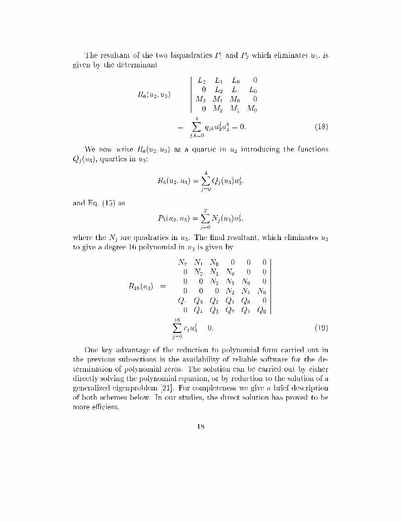
The resultant of the two biquadrati s P1 and P2 whi h eliminates u1, isgiven by the determinantR8(u2; u3) = ��������� L2 L1 L0 00 L2 L1 L0M2 M1 M0 00 M2 M1 M0 ���������= 4Xj;k=0 qjkuj2uk3 = 0: (18)We now write R8(u2; u3) as a quarti in u2 introdu ing the fun tionsQj(u3), quarti s in u3: R8(u2; u3) = 4Xj=0Qj(u3)uj2;and Eq. (15) as P3(u2; u3) = 2Xj=0Nj(u3)uj2;where the Nj are quadrati s in u3. The �nal resultant, whi h eliminates u2to give a degree 16 polynomial in u3 is given byR16(u3) = ��������������N2 N1 N0 0 0 00 N2 N1 N0 0 00 0 N2 N1 N0 00 0 0 N2 N1 N0Q4 Q3 Q2 Q1 Q0 00 Q4 Q3 Q2 Q1 Q0

��������������= 16Xj=0 rjuj3 = 0: (19)One key advantage of the redu tion to polynomial form arried out inthe previous subse tions is the availability of reliable software for the de-termination of polynomial zeros. The solution an be arried out by eitherdire tly solving the polynomial equation, or by redu tion to the solution of ageneralized eigenproblem [21℄. For ompleteness we give a brief des riptionof both s hemes below. In our studies, the dire t solution has proved to bemore eÆ ient. 18

2.1.4 Dire t solution and Sturm hainsWe use the polynomial solution pa kage available from ACM [37℄. Thispa kage uses Sturm's method [15℄ to determine the number of real zeroswithin an arbitrary interval. The intervals are bise ted and re�ned until allthe solutions are put in separate, tight intervals. The solutions are thenre�ned using a se ant method.2.1.5 Generalized eigenproblem formulationThe above polynomial equation an be formulated as a generalized eigen-problem. Following Mano ha [21℄, we write R16(u3) as a determinant of amatrix polynomial with matrix oeÆ ients Sk:det 4Xk=0Skuk3! = 0; (20)whi h is equivalent to det (Bu3 �A) = 0 (21)with B := 0BBB� I 0 0 00 I 0 00 0 I 00 0 0 S4 1CCCA ; A := 0BBB� 0 I 0 00 0 I 00 0 0 I�S0 �S1 �S2 �S3; 1CCCA (22)where all blo ks are of size 6 � 6. The resulting generalized eigenproblem,u1BZ = AZ, an be solved with the LAPACK routine dggev.f, for example.It is also possible to take advantage of the sparsity of the matri es A, B, ifdesired.2.2 Generalizations of the method2.2.1 Non- ontiguous C� atomsAs is lear in Fig. 1, the loop losure pro ess involves three rotations aboutthe axes C�i{C�i+1 (i = 1; 2; 3) and three onstraints relating these rotationsthat ensure that the bond angles between the two rotatable bondsNi{C�i andC�i{Ci at the C�i are set. The hain of atoms intervening between the C�i isrotated rigidly. The problem is ompletely hara terized by giving the angles19

Figure 5: General hain loop losure.�i between the virtual bonds (whi h, together with one of the edges, say C�i{C�i+2, ompletely hara terize the triangle C�i, C�i+1, C�i+2), the angles �i�1,�i formed by the rotatable bonds at ea h C�i and the edges of that triangle,as well as the dihedrals Æi. Nowhere in this onstru tion is any assumptionmade about the intervening stru ture, nor are any su h assumptions impli itin the derivation of the loop losure equations. Therefore the algorithm anbe applied without modi� ation to moves involving arbitrary triads of C�atoms (Fig. 5), i.e., the angle parameters �i, �i, �i, and Æi that ompletelydetermine the problem are de�ned in the same way as in Figs. 3 and 4 (a)from the three atoms at ea h vertex of the C� triangle. This is a new featurerelative to other algorithms. Of ourse more general moves be ome possiblenow, where some of the intervening dihedrals are also hanged, modifying theparameters of the basi triangle. To illustrate this additional exibility we onsider in the next subse tion the simplest su h move, namely the hange ofone additional dihedral. This introdu es a ontinuous DOF to the problem,and it forms the basis of a Monte Carlo move.20

Figure 6: Deformation of C� triangle due to a dihedral (�) perturbation.Changes in �i angles due to the triangle deformation are shown.2.2.2 Additional dihedral angleWe now onsider a method of �nding alternative lo al stru tures when anarbitrary dihedral angle is hanged. Six angles need to be adjusted to om-pensate the hange su h that the hain stru ture is un hanged beyond thelo al region. Con erted angle perturbations of this kind an be used aselementary moves in Monte Carlo simulations to in rease the sampling eÆ- ien y. A simple way is to adjust 6 onse utive angles adja ent to the driverangle [7℄. The terminal atom position is hanged (either C�1 or C�3 in Fig.1) in this ase, and the 6 angle loop losure problem an then be solved withthe hanged C� triangle geometry. Here we des ribe a more general and exible method of ompensating the angle hange, in whi h 6 dihedrals tobe adjusted are allowed to be separated in pairs arbitrarily in sequen e, andthe driver angle an be pla ed anywhere in between the adjusting dihedralpairs.Fig. 6 shows a ase in whi h the driver angle � is pla ed on the lefthand side of the C� triangle, as an example. As before, we onsider three�i rotations separately, and then apply the �i onstraints. This is possiblebe ause the net e�e t of the driver angle rotation in our simpli�ed pi ture21

is to hange some of the parameters for the C� triangle geometry that areindependent of �i rotations. The geometri parameters for the base of thetriangle, C�3C�1; �3; �3, are invariant be ause they are �xed by onstraints,and those for the right side of the triangle, C�2C�3; �2; �2, are also invariantbe ause rotation due to the angles on the left side does not hange the relativeorientation of the atoms on the right. Those for the left side, C�1C�2; �1; �1, hange be ause the driver angle rotates N2 and C�2, but not C�1 and C1.Due to the hange in C�1C�2, zi (i = 1; 2) and �i (i = 1; 2; 3) hange. Eq.(8) an be then derived with the hanged parameters.These exible on erted lo al moves are expe ted to improve eÆ ien y of onformational sear h. A Monte Carlo with Minimization method has beenemployed together with the on erted moves des ribed above, and severalfoldimprovement in eÆ ien y has been observed ompared to existing sear hmethods (See Se tion 3.3).2.3 Bond angle perturbationsSo far we have �xed bond lengths, bond angles, and peptide torsion anglesat their anoni al values in the loop losure algorithm, although there is nolimitation on what spe i� values have to be used. However, real proteinsexhibit a range of values depending on their hemi al environment. When therigid loop losure method is used to sample stru tures for real proteins, somestru tures annot be sampled if the exibility in bonds and angles is ignored.This fa t was �rst noti ed by Bru oleri and Karplus (BK) [24℄. To test howmu h the rigid sampling an over the real protein stru ture spa e, three-residue stru tures were deleted arti� ially from the Top500 database of highresolution, non-redundant protein stru tures [36℄, and our exa t loop losurealgorithm was used to �ll the gaps. About 27.5 % of the gaps ould not be�lled with the rigid sampling. (The bond lengths and angles used are NC� =1:45 �A, C�C = 1:52 �A, CN = 1:33 �A, 6 NC�C = 111:6o, 6 C�CN = 117:5o,and 6 CNC� = 120:0o.) BK developed a sear h method to �nd minimal bondangle variations to lose a given loop. Our method is used to vary peptidetorsion angles as well as bond angles, sin e we now have a more generalformula. We also present a mu h simpler, eÆ ient method of perturbingbond angles, where no extensive sear h is involved.We �rst present a method in whi h the minimum of the polynomial ismoved by angle hanges so that the minimum at least tou hes the axis to giveroots, in a similar spirit to BK. The angles are perturbed by the minimum22

amount (so as to minimize the energy penalty). We then show a fastermethod that makes use of the knowledge of the dire tion of angle hangethat maximizes the probability of having loop losure solutions. This methodonly determines the sign of angle hange, but not the minimum magnitude.2.3.1 Perturbation by angle sear hThe minimum of the polynomial and the derivatives of the minimum withrespe t to perturbed angles are omputed, and a steepest des ent sear h isperformed to bring down the polynomial minimum to equal to or less thanzero. A more sophisti ated LBFGS minimization algorithm was tried, butthe eÆ ien y was similar. The steepest des ent iteration is terminated whenloop losure solutions are found, pre-set maximum angle perturbations arerea hed, or maximum number of iterations (set to 200) is rea hed.The polynomial minimum is obtained by �nding roots of R016(u) = 0and omparing the polynomial values at the roots. The derivatives of theminimum with respe t to perturbed angles are omputed by a �nite di�er-en e method. The minimum at the perturbed angles are omputed by aNewton-Raphson minimization starting from the urrent minimum. Severalparameters are introdu ed to a elerate the steepest des ent iteration. Thestep size of the steepest des ent minimization is in reased or de reased (bya fa tor of fi or fd) depending on whether the previous iteration de reasedor in reased the minimum. The initial step size is hosen so that the largest omponent of angle hange is equal to di. At ea h iteration, the largest angle omponent hange is restri ted to be at most dm. fi = 9, fd = 0:1, di = 0:1,and dm = 0:0001 were hosen by trial and error to maximize the number ofloop losure solutions for the y lopentapeptide example below. It is alsofound that angle perturbations prior to steepest des ent help in �nding moreloop losure solutions. For example, when the C� triangle annot be formedor is formed marginally be ause the base length C�1{C�3 is too short or toolong to be rea hed with the anoni al bond angles, the angles are perturbedby the maximum amount to to allow for longer or shorter base lengths. Inaddition, when it is found that there exists no solution for the two- one sys-tem for any vertex (see Se tion 2.3.2 and Appendix A), angles are adjustedto maximize the overlap of the two- ones as in the next subse tion.23

2.3.2 Simple perturbation methodWe now present a simple bond angle perturbation method that does notrequire sear hing the bond angle spa e, thus solving the loop losure problemonly on e. This an be a omplished by examining the omponents of thesimple pi ture in Fig. 1. Fig. 9 (a) in Appendix A shows �i�1 rotation ofr�i�1 and �i rotation of r�i . Ea h ve tor tra es a one, so we all it a two- one system. The two ve tors have to satisfy the bond angle onstraint Eq.(7), and this limits the a essible ranges of �i�1 and �i values. These rangesdepend on the lo al geometry determined by �i�1, �i, �i, and �i. Ea h vertexof the triangle in Fig. 1 has a two- one system, so there are three two- onesin all. The loop losure solutions are determined by the interse tion of theallowed �i�1/�i regions in the three two- one systems. By onstru tion, �idoes not hange the triangle geometry or any other parameters, but varies thea essible ranges of �i�1/�i. It is possible to determine whether to in rease orde rease �i to maximize the a essible ranges at ea h two- one, whi h in turnmaximizes the overlaps of two- one systems, and the possibility of losing theloop. This is done by lassifying the two- one types depending on how theextrema of �i�1/�i are arranged, and determining the e�e t of �i hange onthe extrema. The details are provided in Appendix A.3 Results and Dis ussionIn this se tion we present an appli ation of the angle perturbation methodin subse tion 3.1, then give two appli ations of the analyti al loop losure,to longer loop modeling and Monte Carlo Minimization, in subse tions 3.2and 3.3, respe tively.3.1 Test of the angle perturbation methodsWe apply the perturbation methods presented in Se tion 2.3 to the three-residue gaps arti� ially deleted from the Top500 stru tures [36℄. When �xed anoni al angle parameters are assumed and the loop losure algorithm isapplied to �ll the three-residue gaps, 22,981 (27.5 %) out of total 83,327gaps don't have loop losure solutions. (Those loops in luding proline havebeen ex luded in this test.) The number of missed gaps de reases dramat-i ally with the simple perturbation method of Se tion 2.3.2: 1,249 (1.5 %)and 469 (0.56 %) with the maximum angle variation of 5 and 10 degrees,24

respe tively. Note that only 3 NC�C angles have been varied here. The fullangle perturbation of Se tion 2.3.1 misses 209 (0.25 %) and 23 (0.028 %)for the maximum allowed perturbation 5 and 10 degrees, respe tively, when9 angles are varied (3 NC�C, 2 C�CN , 2 CNC�, and two peptide torsionangles). In summary, the simple perturbation method is su essful in over-ing most of the onformational spa e realized in the database, and the fullangle perturbation an push the limit to almost perfe tion. Computationtime in reases only a few per ent even with the full sear h method for thistest be ause most of the loops have solutions, and only a few iterations areneeded for angle sear h. Computation time in reases more with perturba-tions when there are more ases in whi h loop losure solutions are not foundsu h as when applied to loop modeling or for exhaustive sampling as in the y lopentapeptide example below.Next we onsider the y lopentapeptide Gly-Gly-Gly-Pro-Pro examplefor whi h G�o and S heraga [38℄ and Bru oleri and Karplus [24℄ sampledthe onformational spa e. The two Pro � angles are frozen, the two Pro angles are varied with a grid of 5 deg, and the remaining 6 Gly �/ torsionsare solved for. We use the same bond lengths and angle parameters asBK, and 346 loops are losed when no perturbation is used. BK losed1,507 and 1,565 loops with their fast and slow bond angle sear h method,respe tively, varying 9 bond angles with maximum variation of 5 degrees. Ourfull perturbation method loses 1,517 loops when the same 9 angles (3NC�C,3 C�CN , 3 CNC�, in luding two bond angles outside the C� triangle) arevaried with the same 5 degree maximum variation. In luding perturbationsin the additional 3 peptide torsional angles loses 1,594 loops. Our full sear hmethod is thus omparable to that of BK in the number of losed loops, andour ability to add the peptide torsion DOFs in reases the overage of the onformational spa e slightly. The simple 3-angle perturbation loses 819 losed loops, whi h is twi e as many as those obtained without perturbation(346), but only half of those obtained with full perturbation. The total omputation time in reases steeply with in reasing perturbation level: 0.26,0.56, 17.6, and 24.0 se onds for no perturbation, simple 3-angle perturbation,9-angle, and 12-angle perturbations, respe tively, when s aled to an AMD1800+ MP pro essor.25

3.2 Appli ation to loop modelingAnalyti al loop losure �nds a dis rete set of loop onformations for a threeresidue loop, but a longer loop has a ontinuous set of possible losed loop onformations. Sampling a longer loop therefore requires a strategy to samplethe extra DOFs to be oupled with the analyti al loop losure. The extraDOFs ould be sampled either randomly or in an informed way. When thesampling is random, unfeasible onformations due to unfavorable �/ anglesor steri lashes would be s reened out in later stages of loop predi tionalgorithms, but it would be more eÆ ient if su h stru tures are ex ludedduring the loop sampling stage. We employ an existing loop onstru tionalgorithm [31℄ whi h performs this by sampling in the allowed regions of the�/ map in a dis rete manner and s reening possible side hain lashes usinga rotamer library. This algorithm (as implemented in the program PLOP[31℄) is used to build the N-terminal and the C-terminal bran hes ex ept forthe three residue gap in the middle of a loop, and the analyti al loop losurealgorithm is used to lose the bran hes.The performan e of our oupled algorithm is ompared to the re ent workof Canutes u and Dunbra k alled CCD ( y li oordinate des ent) [39℄. TheCCD algorithm is a numeri al loop losure algorithm whi h is similar in spiritto the \random tweak" method [29℄, solving �rst-order equations iteratively,but it is more robust and eÆ ient. We take the same test set as in Table 2 ofRef. [39℄, whi h onsist of 10 loops ea h with lengths of 4, 8, and 12 residues(total of 30 loops) hosen from a set of non-redundant X-ray rystallographi stru tures. The omparison is summarized in Table I. The average of the bestba kbone RMSD obtained from CCD is 0.56, 1.59, and 3.05 �A for 4, 8, and12 residue loops, respe tively, with average omputing time per losed loopof 31, 37, and 23 millise onds on an AMD 1800+ MP pro essor. Our oupledalgorithm gives better average minimum RMSDs of 0.40, 1.01, and 2.34 �A,in almost two orders of magnitude less omputing time (0.56, 0.68, and 0.72millise onds per loop when s aled to the same pro essor). In addition, theminimum RMSD for individual test loops is better for 25 out of the 30 asesin Table I. The onditions under whi h we perform the omparison a tuallydisfavor our algorithm be ause we generate fewer loops. With CCD, theloops are obtained from 5000 trials (thus about 5000 loop andidates, giventhat the algorithm an lose the loops 99.8 % of the time). However with ouralgorithm, the exa t number of loop andidates is not the ontrol parameterof the algorithm but rather the sampling resolution in the �/ map. As the26

4 residue loops 8 residue loops 12 residue loopsLoop CSJD CCD Loop CSJD CCD Loop CSJD CCD1dvjA 20 0.38 (4548) 0.61 1 ruA 85 0.99 (2516) 1.75 1 ruA 358 2.00 (4148) 2.541dysA 47 0.37 (2234) 0.68 1 tqA 144 0.96 (1754) 1.34 1 tqA 26 1.86 (3968) 2.491eguA 404 0.37 ( 170) 0.68 1d8wA 334 0.37 (1686) 1.51 1d4oA 88 1.60 (1802) 2.331ej0A 74 0.21 (1564) 0.34 1ds1A 20 1.30 (3506) 1.58 1d8wA 46 2.94 (3906) 4.831i0hA 123 0.26 ( 342) 0.62 1gk8A 122 1.29 (2362) 1.68 1ds1A 282 3.10 (1162) 3.041id0A 405 0.72 ( 528) 0.67 1i0hA 145 0.36 (1452) 1.35 1dysA 291 3.04 (2306) 2.481qnrA 195 0.39 (1064) 0.49 1ixh 106 2.36 (4448) 1.61 1eguA 508 2.82 (2106) 2.141qopA 44 0.61 (4284) 0.63 1lam 420 0.83 (2200) 1.60 1f74A 11 1.53 (3048) 2.721t a 95 0.28 ( 418) 0.39 1qopB 14 0.69 (3384) 1.85 1qlwA 31 2.32 (4780) 3.381thfD 121 0.36 (2958) 0.50 3 hbD 51 0.96 (1838) 1.66 1qopA 178 2.18 (2014) 4.57Average 0.40 (1181) 0.56 Average 1.01 (2525) 1.59 Average 2.34 (2924) 3.05Table 1: Minimum RMSD (in �A) of the andidate loops with our algorithm(CSJD) and the CCD algorithm. CCD results are taken from Table 2 ofRef. [39℄. 5000 trials were performed per test loop with the CCD, so theminimum is among about 5000 losed loops. With CSJD, the number of andidate loops is taken to be always less than 5000 for ea h test loop, andshown in the parentheses.sampling resolution is in reased, the number of loop onformations in reases.For this omparison, we generate less than 5000 loop andidates for ea h test ase, sometimes far less, whi h disfavors us in the omparison. The numberof loop andidates for ea h test loop is also shown in Table I.The oupled algorithm is also ompared with the algorithm as presentedin Ref. [31℄ whi h does not use the analyti al loop losure and ontinues thedis rete �/ sampling instead to lose the loop, whi h we all \numeri al" losure here. When the same resolutions, thus the same sets of onformationsfor the residues outside of the 3-residue losure segment, are used, the aver-age best RMSD obtained is 0.29, 1.66, and 3.25 �A with omputation timeper loop of 0.73, 1.60, and 106 millise onds. Ex ept for the short 4-residueloops, whi h are easy both for the numeri al and analyti al losure due to thesmall number of DOFs, the analyti al losure gives better RMSD in ordersof magnitude shorter time per loop onformation, espe ially for the longest12 residue loops. This is expe ted be ause the analyti al losure an losebran hes more eÆ iently for the given sampling resolution for the bran hes.The number of onformations generated by the analyti al losure method(whi h in essen e has in�nite sampling resolution) is mu h higher than thenumber generated by the algorithm without analyti al losure. The averagenumber of losed loops with the numeri al losure is 459, 236, and 42 for the4, 8, and 12 residue loops, respe tively, ompared to 1181, 2525, and 292427

with the analyti al losure at the �xed bran h sampling resolutions. In thetests performed here, in whi h the maximum number of loop andidates isheld �xed at 5000, this is a tually disadvantageous for the analyti al losure,be ause more loops are generated using oarser sampling for the non- losureresidues. When a maximum of 5000 loops are generated, the numeri al lo-sure thus gives better RMSD (0.27, 1.04, and 1.89 �A) although with longer omputing time per loop (8.5, 6.1, and 23 millise onds). This implies thatthe optimal number of losed loops to be sampled is di�erent for the analyt-i al and numeri al losure, and more loop andidates must be sampled withthe analyti al losure. Clustering algorithms an be used to remove the re-dundan ies in the andidates before more expensive re�nement and res oringsteps [31℄.Finally, adding the bond angle perturbations is found not to a�e t thebest RMSD ompared to no perturbation, although more losed loops arefound. Produ ing more high quality loops by a biased perturbation thatsamples desired regions of �/ would be more useful for loop modeling.3.3 Appli ation to loop optimization using Monte CarloMinimizationWe employ the lo al moves des ribed in Se tion 3.2 as a perturbation strategyin the Monte Carlo Minimization (MCM) method of Li and S heraga [40℄,and apply the method to the global energy minimization of a protein loop.MCM is a global optimization method by whi h lo al energy barriers anbe over ome with energy minimization of the perturbed stru ture before aMetropolis riterion [41℄ is applied.We now take advantage of the fa t that some steri barriers that arehard to over ome by random moves of individual atoms ould be bypassedby oordinated moves of multiple atoms. It has been reported that addingsu h on erted moves in Metropolis Monte Carlo simulations improves thesampling eÆ ien y [2, 3, 5, 6, 7℄. Our lo al moves are more general than thosepreviously applied to MC simulations, but it is straightforward to apply thesemoves to MC. The same Ja obian as in [3, 7℄ needs to be in luded to satisfythe mi ros opi reversibility. Here we apply the on erted moves to MCMfor the �rst time, and show signi� ant improvement in eÆ ien y in �ndingthe global minimum.Several other strategies for lo al moves have been applied to the loop28

optimization problem (see referen es in Ref. [42℄), and among these, Lo alTorsional Deformation (LTD) [42℄ has been one of the most eÆ ient methodsof perturbing y li or loop stru tures when ombined with MCM. In LTD,torsion angles are perturbed only lo ally, i.e., no bonds are rotated beyond theperturbed region. In addition, only those perturbations that keep the bondbetween the last perturbed atom and the �rst unperturbed atom within aring losure range (0.5 - 3.5 4 �A) are onsidered [42℄. In our approa h, onetorsion angle (� or ) in the loop is perturbed, and six other torsion angles(three pairs of � and ) are adjusted to keep the perturbation lo al. Theperturbed onformations thus do not have any large strains due to unrealisti bond angles or bond lengths. Su h a move is ompared with LTD below.3.3.1 ResultsIt is not intuitively obvious whether using perturbations exa tly satisfyinggeometri al onstraints (Exa t Loop Closure, ELC) would be signi� antlymore eÆ ient than approximate perturbations like LTD, be ause a physi alenergy fun tion an orre t for the ina urate geometry in the pro ess ofenergy minimization. Figs. 7 and 8 show that the moves based on our ex-a t loop losure (ELC) a tually greatly enhan e the performan e of MCM ompared to approximate LTD in �nding low energy onformations. Fig. 7illustrates that ELC �nds the (putative) global minimum about three timesfaster than LTD, and Fig. 8 shows that ELC has a mu h higher probability of�nding the orre t global minimum than LTD when the optimization startswith a random initial stru ture. The details on the simulations are presentedin Se tion 3.3.2.If keeping the ba kbone geometry within physi ally reasonable rangesimproves eÆ ien y, the same is expe ted for side hains. We thus draw theside hain torsion angles from a rotamer library. The rotamer probabilitydistributions in the ba kbone dependent rotamer library of Dunbra k et al[43℄ are used to perturb side hain torsion angles. This rotamer methodis ompared with \random" side hain perturbation method. Employing arotamer library improves the performan e: average lowest energies foundafter 10 runs of 1000 MCM iterations with rotamer and random methodsare respe tively, -2478.5 and -2477.2 k al/mol for ELC, and -2473.2 and -2463.7 k al/mol for LTD for the same initial loop stru ture as in Fig. 7.Computations in Figs. 7 and 8 were both performed with the side hainrotamer library. 29

0 200 400 600 800 1000

Iteration

-2480

-2470

-2460

-2450

-2440

-2430

-2420

Ene

rgy

(kca

l/mol

)

ELCLTD

Figure 7: ELC �nds the putative global energy minimum more eÆ ientlythan LTD. 10 MCM runs (1000 iterations, or minimizations, for ea h) areshown. Ea h run starts from the same initial onformations, whi h is 3.8 �Afrom the rystal stru ture. The ordinate represents the lowest energy foundup to that iteration number.

30

0 1 2 3 4 5 6

RMSD

-2500

-2450

-2400

-2350

Ene

rgy

(kac

l/mol

)

ELCLTD

Figure 8: ELC �nds lower energy and rmsd stru tures than LTD when MCMis started from diverse initial stru tures. The ordinate and abs issa are thelowest energy found and RMSD orresponding to the stru ture. The ini-tial stru tures are generated by randomly hoosing �/ angles of the loopresidues. 1000 iterations were performed for ea h of 30 random initial stru -tures. Only 23 points are shown for LTD be ause 7 other points have mu hhigher energy and rmsd.31

3.3.2 MethodsThe energy fun tion used is EEF1 [44℄ whi h is the CHARMM 19 polarhydrogen for e �eld with a Gaussian impli it solvation model. An 8-residueloop (84-91) in Turkey egg lysozyme (pdb ode 135l.pdb) is taken for thisstudy be ause the (putative) global minimum of this loop is lo ated very lose to the rystal stru ture (about 0.3 �A). The loop RMSD is measured asthe root mean square deviation in the main hain atoms of the loop when thethree stem residues on both sides of the loop are optimally superimposed.The L-BFGS-b algorithm [45℄ by Zhu et. al. is used for energy minimizationwith the gradient toleran e of 1 k al/mol�A.The details of modeling and parameters for both ELC and LTD are asfollows. Hydrogen atoms are modeled on the rystal stru ture and the stru -ture is energy minimized to remove bad onta ts with harmoni onstrainson heavy atoms with the for e onstant 5 k al/mol. The resulting stru tureis 0.1 �A from the rystal stru ture. All other atoms are �xed ex ept forthe loop atoms in MCM. The temperature parameter kT for MCM is setto 1 k al/mol for both ELC and LTD. In ELC, we hoose three residues inthe loop randomly whose �/ angles ompensate for the hange of a drivertorsion angle, whi h is also hosen randomly within the triangle formed bythe three residues. The driver angle � is hanged with uniform probabilityin the range [� � f1�, � + f1�℄. f1 = 0:7 was found to be optimal. Out ofthe multiple loop losure solutions, the losest solution to the urrent stru -ture in RMSD is sele ted for the perturbation step in MCM. In LTD, four onse utive �/ angles are perturbed with uniform probability in the range[�� f2�, �+ f2�℄, where f2 = 0:8 was found to be optimal. We also tried 3-4one or two onse utive angle movements following Ref. [42℄, but they wereless eÆ ient. However, it has to be mentioned that omparisons of algo-rithms is not always straightforward, with a lot of parameters and te hni aldetails that an be varied. For both LTD and ELC, ea h side hain is per-turbed independently with the probability 1/8, and the side hain rotameris sele ted from the ba kbone dependent rotamer library with the ba kbonedependent probability. The random side hain perturbation method perturbsea h side hain torsion angle independently with the probability 1/8, and theangle value is drawn from a uniform range around the urrent value [�� f�,�+ f�℄, where f = f1 for ELC and f = f2 for LTD.32

4 Con lusionsThe bonded near-neighbor for es in a protein an be grouped into roughlythree ategories with respe t to strength: hard for es asso iated with bondlengths, intermediate for es asso iated with bond angles, and soft for es as-so iated with the �/ dihedrals and side hain angles. The for es asso iatedwith the ! dihedral of the peptide bond an be pla ed in the intermediaterange. In onsidering a polypeptide hain it is tempting to on entrate onmotions asso iated with the \soft" DOFs, i.e., those asso iated with �/ .The other DOFs an be assumed to vary to a limited degree, although they an be �xed to arbitrary values as far as the geometri analysis is on erned.The onformational spa e of a tripeptide unit (ex luding N1 and C3) anbe seen as the Cartesian produ t of two ir les, i.e., a torus. Exploring the onformation spa e of this simple system is straightforward in terms of the�/ dihedrals. However, adding a onstraint su h as �xing the distan ebetween C�1 and C�3 introdu es a relationship between the two dihedrals,Eq. (11), and this interdependen e (\Rotation Transfer Fun tion" or RTF)forms the basis of the analyti al approa h followed in this paper. In general,�xed-distan e onstraints, whether resulting from NMR measurements forstru ture determination or as part of a strategy for exploring onformationspa e, imply sets of su h transfer fun tions among angle DOFs and, when ombined with the other \almost-rigid" onstraints in a ma romole ule, leadto a redu tion in the dimensionality of the spa e of allowed motions. Al-lowing for small variability of additional DOFs provides a sear h algorithmwith more room to maneuver, repla ing barriers by narrow, passable orri-dors. Su h onstraint- ompatible onformations form the natural low-energyterrain that needs to be explored thoroughly. Choosing oordinates that de-s ribe this terrain eÆ iently, is an essential part of this exploration, sin e theredu tion in dimension omes at the pri e of ompli ated topology. Clearly,these ideas need not be limited to ba kbone motions, and extending themto side hains is essential if NMR derived distan e onstraints are to be in- luded. In that regard we view the tripeptide loop losure and the variantspresented here as one of many possible appli ations of the distan e-anglerelationship expressed by the basi RTF.Several generalizations of the method presented here are possible. Forexample, the transfer fun tions are Fourier polynomials in the other anglevariables as well. A redu tion of these to polynomial form would lead to anew polynomial system, now in several additional variables. The zero sets33

be ome higher dimensional obje ts and new methods an be brought to bearfor �nding losure solutions. We hose to treat these variables by simplesear h methods here, but a more omplete sear h would be required if forexample some energy riterion is in luded in the perturbation pro ess.The main advantage of a �= sear h method is that it avoids sear hing onformations that introdu e distortions of the hard DOFs. The bene�t ofthe method in redu ing the size of the sear h spa e is not seriously a�e tedif small variations in additional DOFs are allowed. Thin slivers of on�gura-tions repla e the �= hypersurfa es, so that the volume of the allowed spa eis still dramati ally redu ed. In order to take full advantage of the intimate onne tion between the on erted moves idea and the true kinemati DOFsof the hain, a strategy of hoosing moves should be informed about the e�e tof these moves vis. steri lashing with the rest of the hain as well as side hain pla ement. A possible extension ould be the in orporation of obsta leavoidan e and other similar ideas from roboti motion planning.A Two- one systems and the Rotation Trans-fer Fun tionIn the body frame of the three �xed C�i atoms, the C�iNi unit ve tor r�i�1and the C�iCi unit ve tor r�i lie on ones about the C�i�1C�i and C�iC�i+1virtual bonds, respe tively, assuming �xed bond lengths, angles, and dihedral!. See Fig. 9 (a) The �i�1 and �i rotations are not independent be ause thebond angle NiC�iCi must be �xed (or in a limited range in general). If we anthink of the ones of possible lo ations of the bonds about their orrespondingvirtual axes, then we must think of the angle onstraint between the twobonds as a �xed distan e ondition between two generatri es of these onesas shown in Fig. 9 (a). Clearly, to ea h position of one bond there an beat most two positions for the other. Sin e the four angles �; �; �; � are onstant, the alternative positions des ribe the possible onformations of thetetrahedral formed by these four angles in Fig. 9 (b).The ranges of these positions an hange hara ter and transit from bothhaving one onne ted omponent (Fig. 10 (a)) to where one of them splitsto two disjoint arms (Fig. 10 (b)).At ea h two- one, the �i�1 and �i rotations are related by the �i bond34

Figure 9 (a): The two ones at a double rotatable bond jun tion. The bla k ir le denotes the C� atom, the bla k oval on the � - one the end of the C�Cunit ve tor, and that on the �- one the end of C�N unit ve tor. The dashedlines are the virtual bonds between the C� atoms, and the line between theovals shows the �xed distan e onstraint.35

Figure 9 (b): The angles at a double rotatable bond jun tion36

Figure 10 (a): A type of two ones (type IIb) in whi h both C (on the � - one)and N (on the �- one) tra e onne ted segments. The bla k ir les denoteextreme positions of the N and C atoms. The white ir le is the C position orresponding to the N at the bla k ir le onne ted to it by a line.37

Figure 10 (b): A two- one type (type IIIb) in whi h the C atom (on the� - one) tra es two disjoint segments, and N (on the �- one) tra es the whole ir le.

38

angle onstraint r�i � r�i�1 = os �; (23)whi h results in Eq. (8) rewritten omitting subs ripts for simpli ity: os � + os � os � os� =sin�(sin � os � os � + os � sin � os �)+ sin � sin �(sin � sin� + os� os � os �): (24)To see the �{� relation more expli itly, � := �i is solved for given � :=�i�1, or � given � . Arranging Eq. (24) as at os � + bt sin � = t gives� = �o � ar os( t=qa2t + b2t ); (25)where at = os� sin � sin � os � + sin� os � sin �;bt = sin � sin � sin�; t = os � + os� os � os � � sin� sin � os � os �; os �o = at=qa2t + b2t ;sin �o = bt=qa2t + b2t : (26)Given � , � is expressed as� = �o � ar os( s=qa2s + b2s); (27)where as = os� sin � sin � os � + sin� sin � os �;bs = sin � sin � sin �; s = os � + os� os � os � � sin� os � sin � os �; os �o = as=qa2s + b2s;sin�o = bs=qa2s + b2s: (28)Eq. (25) has two solutions if j t=qa2t + b2t j < 1, one if = 1, and none if> 1. The range of � in whi h solutions exist is determined by �1 and �239

whi h are two roots of 2t = a2t + b2t , and likewise for � . The roots an alsobe found by noting the following geometri al relations:r�i�1 � zi = os(� � �);r�i � zi�1 = � os(� � �); (29)whi h give os(� � �) = sin� sin � sin�� os � os�; (30) os(� � �) = sin � sin � sin�� os � os�: (31)Eqs. (30) and (31) have roots if the following onditions are satis�ed:[ os(� � �) + os(� + �)℄[ os(� � �) + os(�� �)℄ � 0; (32)[ os(� � �) + os(� + �)℄[ os(� � �) + os(�� �)℄ � 0: (33)We all the roots of Eqs. (30) and (31) �� and ��. When there exist roots,there are six two- one types depending on the sign (�) of ea h root.I. No solutionIIa. �+, �+IIb. ��, ��IIIa. �+, ��IIIb. �+, ��IVa. �+, ��IVb. ��, �+It an be seen that in the ase of IIa, in reasing � in reases the allowablerange of �/� , and de reasing � in reases the range for IIb (See Fig. 10 (a)).This fa t is used in the simple perturbation method des ribed in Se tion2.3.2. For other two- one types, the � values are in reased in the perturbationalgorithm.The �i�1{�i relationship is more ompli ated than the �i{�i relationship(�i = �i + Æi), but more detailed understanding of the �{� relationship atthe jun tion of the two rotatable bonds is useful. First, it makes it possible40

to predi t the e�e t of bond angle perturbations, as des ribed in Se tion 4.2.Se ond, it also reveals the geometri al restri tion on the side hain lo ation,espe ially C�, due to the orrelated movement of Ni, C�i, and Ci atoms asdes ribed by orrelation of the �i�1 and �i rotations. To demonstrate this,in Fig. 10, we show the �{� relationship and the orresponding C� positionsobtained from the anoni al tripeptide geometry, and ompare with thoseextra ted from the stru ture database Top500 [36℄. Figs. 11 (a) and 11 (b)show possible ranges for �{� and C� when � is �xed at 90o (this value of � hasthe maximum density in the � distribution in the database). The databasepoints are for � = 90 � 0:5o. Clearly the theoreti al �{� urve omputedfrom the anoni al bond angles shows ex ellent agreement with the databasepoints, the large majority of stru tures lustering about the Rama handranallowable portion of the �{� urve. (Fig. 11 (a)) Re onstru ting C� using anoni al angles shows also lose agreement. (Fig. 11 (b)) This is the uni-modal ase (also illustrated in Fig. 10 (a)) and it is the most ommonlyo urring on�guration in the database. Figs. 11 ( ) and 11 (d) show an ex-ample of a bimodal ase (also illustrated in Fig. 10 (b)), for � = 111o, whi his lose to the se ond density maximum in the distribution of �. Here wesee a small dis repan y, indi ating that the stru ture is stressed, i. e., someof the parameters are o� their typi al values. The stress turns out to beeven stronger if one ompares the C� distribution in the database to that re- onstru ted assuming typi al angle values. We are studying these propertiesfurther, together with their possible appli ation to side hain optimizationespe ially when ba kbone exibility is also taken into a ount.B CoeÆ ients of the polynomialsEq. (8) is written as a double Fourier series0 = ai + bi os �i�1 + i os �i+ di os �i�1 os �i + ei sin�i�1 sin �i ; (34)where the oeÆ ients areai = � os �i � os �i os �i�1 os�ibi = sin�i sin �i�1 os �i i = sin�i os �i�1 sin �i41

-200 -150 -100 -50 0 50

σ

-200

-150

-100

-50

0

τ

All rangeRamachandran allowedFrom Database

Figure 11 (a): The �{� relationship given by the Rotation Transfer Fun tionfor � = 90o and typi al values of � = 111:6o; � = 16:63o; � = 19:13o, plottedtogether with �-� values in the database.

42

-180 -160 -140 -120 -100 -80

φβ

0

10

20

30

40

50

60

70

θ β

All rangeRamachandran allowedFrom Database

Figure 11 (b): Plot of the lo ation of C� as omputed from the �{� values inthe theoreti al urve of Fig. 11 (a), against C� positions from the database,both shown in spheri al oordinates.

43

-200 -100 0 100 200 300

σ

-300

-200

-100

0

100

200

τ

No perturbation5 deg perturbation-5 deg perturbationFrom Database

Figure 11 ( ): Same as Fig. 11 (a), but for � = 111o. Two more urves with� perturbation of 5o and �5o are shown together, whi h improve �t to thedatabase points. The ase is bimodal, although its hara ter shifts as � is hanged.

44

-200 -180 -160 -140 -120 -100

φβ

0

20

40

60

80

100

θ β

No perturbation5 deg perturbation-5 deg perturbationFrom Database

Figure 11 (d): The C� plots orresponding to the situation in Fig. 11 ( ).di = os�i sin �i�1 sin �iei = sin �i�1 sin �i :Now introdu e the half-angle formulas Eq. (9, 10) into (34) to arrive ata system of three biquadrati s in wi, ui, i = 1; 2; 3;0 = ai + bi 1� w2i�11 + w2i�1 + i1� u2i1 + u2i+ di1� w2i�11 + w2i�1 1� u2i1 + u2i + ei 2wi�11 + w2i�1 2ui1 + u2i ;or equivalently:0 = ai(1 + w2i�1)(1 + u2i ) + bi(1� w2i�1)(1 + u2i ) + i(1 + w2i�1)(1� u2i )+ di(1� w2i�1)(1� u2i ) + ei4wi�1ui;Expanding and regrouping results in Eq. (11):Aiw2i�1u2i +Biw2i�1 + Ciwi�1ui +Diu2i + Ei = 0 (35)45

where Ai = ai � bi � i + di = � os �i � os (�i � �i�1 � �i)Bi = ai � bi + i � di = � os �i � os (�i � �i�1 + �i)Ci = 4ei = 4 sin �i�1 sin �iDi = ai + bi � i � di = � os �i � os (�i + �i�1 � �i)Ei = ai + bi + i + di = � os �i � os (�i + �i�1 + �i) :We now eliminate the variables wi: using the twist transformation, Eq. (12),wi = ui +�i1��iui ; �i = tan Æi=2 ;in Eq. (35) we �ndAi ui�1 +�i�11��i�1ui�1!2 u2i+Bi ui�1 +�i�11��i�1ui�1!2+Ci ui�1 +�i�11��i�1ui�1ui+Diu2i+Ei = 0(36)Finally, the derivation of the oupled biquadrati polynomials Eqs. (13),(14), and (15), is arried out by multiplying through by (1��i�1ui�1)2 andregrouping. Sin e � = sin Æ1 + os Æ ; �2 = 1� os Æ1 + os Æ ;we multiply the resulting expressions through by (1+ os Æi�1)=2 to arrive atthe expression for the oeÆ ients:p(i)22 = � os �i � os �i�1 os (�i � �i)� os Æi�1 sin �i�1 sin (�i � �i)p(i)21 = �2 sin Æi�1 sin �i�1 sin �ip(i)20 = � os �i � os �i�1 os (�i + �i)� os Æi�1 sin �i�1 sin (�i + �i)p(i)12 = �2 sin Æi�1 sin �i�1 sin (�i � �i)p(i)11 = 4 os Æi�1 sin �i�1 sin �ip(i)10 = �2 sin Æi�1 sin �i�1 sin (�i + �i)p(i)02 = � os �i � os �i�1 os (�i � �i) + os Æi�1 sin �i�1 sin (�i � �i)p(i)01 = 2 sin Æi�1 sin �i�1 sin �ip(i)00 = � os �i � os �i�1 os (�i + �i) + os Æi�1 sin �i�1 sin (�i + �i) :46

Eqs. (13), (14), and (15) are now rewritten asP1(u3; u1) = 2Xk=00� 2Xj=0 p(1)jk uj31Auk1 = 2Xk=0Lkuk1;P2(u1; u2) = 2Xj=0 2Xk=0 p(2)jk uk2!uj1 = 2Xj=0Mjuj1;and P3(u2; u3) = 2Xj=0 2Xk=0 p(3)jk uk3!uj2 = 2Xj=0Njuj2;where Lk := Lk(u3) := 2Xj=0 p(1)jk uj3;Mj :=Mj(u2) := 2Xk=0 p(2)jk uk2;and Nj := Nj(u3) := 2Xk=0 p(3)jk uk3:The resultant of P1 and P2, whose vanishing guarantees a ommon rootin u1, is given by the determinantR8(u2; u3) = ��������� L2 L1 L0 00 L2 L1 L0M2 M1 M0 00 M2 M1 M0 ���������= ����� L2 L0M2 M0 �����2 � ����� L2 L1M2 M1 ����� ����� L1 L0M1 M0 �����Sin e all the non-vanishing elements are produ ts of two quadrati s in u2 andtwo quadrati s in u3, the resultant is a biquarti in these variables, and hasthe form R8(u2; u3) = 4Xj;k=0 qjkuj2uk3 :Here, the 5 � 5 = 25 quantities qjk are found in terms of produ ts of theajk := p(1)jk and bjk := p(2)jk by expressing R8 as a sum of six tensor produ ts.47

We write R8 as a quarti in u2 introdu ing the fun tions Qj, quarti s inu3: R8 = 4Xj=0 4Xk=0 qjkuk3!uj2 =: 4Xj=0Qjuj2 :The �nal resultant, whi h eliminates u2 to arrive at a degree 16 polynomialin u3 is given by: R16 = det(S)where the matrix S is given as:S(u3) := 4Xk=0Skuk3 = 0BBBBBBBB� N2 N1 N0 0 0 00 N2 N1 N0 0 00 0 N2 N1 N0 00 0 0 N2 N1 N0Q4 Q3 Q2 Q1 Q0 00 Q4 Q3 Q2 Q1 Q01CCCCCCCCA (37)so that Sk := 0BBBBBBBB� 2k 1k 0k 0 0 00 2k 1k 0k 0 00 0 2k 1k 0k 00 0 0 2k 1k 0kq4k q3k q2k q1k q0k 00 q4k q3k q2k q1k q0k

1CCCCCCCCA(where we de�ned ij := p(3)ij , with i3 = i4 = 0, i = 0; 1; 2). These matri es an be used dire tly in the matrix polynomial approa h whi h �nds thesolutions as eigenvalues of a " ompanion" matrix pen il. The omputationof the polynomial oeÆ ients for the dire t approa h requires some additional omputations des ribed below. We pro eed by a Lapla e expansion [46℄ ofEq. (37) by omplementary minors of order 3. First we rearrange the rowsof S:detS = ��������������N2 N1 N0 0 0 00 N2 N1 N0 0 00 0 N2 N1 N0 00 0 0 N2 N1 N0Q4 Q3 Q2 Q1 Q0 00 Q4 Q3 Q2 Q1 Q0

�������������� = � ��������������N2 N1 N0 0 0 0Q4 Q3 Q2 Q1 Q0 00 0 N2 N1 N0 00 N2 N1 N0 0 00 Q4 Q3 Q2 Q1 Q00 0 0 N2 N1 N0 :

��������������= � X1�i1<i2<i3�6(�1)i1+i2+i3 detS(1; 2; 3; i1; i2; i3) detS(4; 5; 6; i4; i5; i6)48

where S(1; 2; 3; i1; i2; i3) is the 3 � 3 submatrix of S formed by elements inrows 1; 2; 3 and olumns i1 < i2 < i3. Also, i4 < i5 < i6 and i3; i4; i5 di�erfrom i1; i2; i3. We introdu e the 3� 5 submatrixP := 0B� N2 N1 N0 0 0Q4 Q3 Q2 Q1 Q00 0 N2 N1 N0 1CAand the 3� 3 minors T (i; j; k) formed by the olumns i, j and k of P . Then,the Lapla e expansion of S in terms of the minors based on rows 1,2,3 andtheir omplements from rows 4,5,6 [46℄ an be written ompa tly in the form:detS = T (1; 2; 3)T (3; 4; 5)� T (1; 2; 4)T (2; 4; 5) + T (1; 2; 5)T (2; 3; 5)+ T (1; 3; 4)T (1; 4; 5)� T (1; 3; 5)T (1; 3; 5) + T (1; 4; 5)T (1; 2; 5)The omputation of the resultant pro eeds with the 9 quantities T (i; j; k)above. Sin e they are sums of produ ts of terms of the form N�N�Q theyare polynomials in u1 of degree 8. We list the expressions for these belowin terms of the Ni; Qj involved. On e the T 's have been omputed, we needto ompute the produ ts above, i.e. we need to ompute 6 binary produ tsof polynomials of degree 8. A ertain amount of fa toring an be utilized tofurther redu e the operational ount of this pro edure.We give now the T (i; j; k):T (1; 2; 3) = ������� N2 N1 N0Q4 Q3 Q20 0 N2 ������� = N2 ����� N2 N1Q4 Q3 �����T (1; 2; 4) = ������� N2 N1 0Q4 Q3 Q10 0 N1 ������� = N1 ����� N2 N1Q4 Q3 �����T (1; 2; 5) = ������� N2 N1 0Q4 Q3 Q00 0 N0 ������� = N0 ����� N2 N1Q4 Q3 �����T (1; 3; 4) = ������� N2 N0 0Q4 Q2 Q10 N2 N1 ������� = �N2 ����� N2 N1Q2 Q1 ������Q4N0N1T (1; 3; 5) = ������� N2 N0 0Q4 Q2 Q00 N2 N0 ������� = �N2 ����� N2 N0Q2 Q0 ������Q4N2049

T (1; 4; 5) = ������� N2 0 0Q4 Q1 Q00 N1 N0 ������� = �N2 ����� N1 N0Q1 Q0 �����T (2; 3; 5) = ������� N1 N0 0Q3 Q2 Q00 N2 N0 ������� = �N1 ����� N2 N0Q2 Q0 ������N20Q3T (2; 4; 5) = ������� N1 0 0Q3 Q1 Q00 N1 N0 ������� = �N1 ����� N1 N0Q1 Q0 �����T (3; 4; 5) = ������� N0 0 0Q2 Q1 Q0N2 N1 N0 ������� = �N0 ����� N1 N0Q1 Q0 �����From these expressions, whose omputation involves only 4 distin t 2 � 2determinants, we an ompute the �nal polynomial. This omputation anbe done analyti ally, by deriving the lengthy expressions for the oeÆ ientsof the �nal polynomial in terms of the oeÆ ients of the original polynomi-als. These analyti al expressions an be useful, espe ially if one wants tostudy the e�e t of varying parameters on the behavior of the solution of thetripeptide loop losure. For the al ulations reported in this paper, the om-putation of the oeÆ ients was done numeri ally. In this ase, it is optimalto ompute the 8-th degree polynomials asso iated with ea h of the T (i; j; k)and then ompute the 6 polynomial produ ts (whi h an be easily redu edto 5 polynomial multipli ations with appropriate fa torizations).C Systems of polynomials and ResultantsThe resultant of a system of polynomials in several variables is a ne essaryand suÆ ient ondition for the existen e of a ommon solution. For twopolynomials, Fm(u) and Fn(u) of degreesm and n, to have a ommon solutionu they must have a fa tor in ommon, i.e. there must exist polynomials g(u)and h(u) of degrees � n� 1 and � m� 1 respe tively su h thatgFm + hFn = 0 :This leads to a system ofm+n linear homogeneous equations for determiningthe oeÆ ients of g and h, and the resultant is the determinant of the matrix50

asso iated with that system. We demonstrate how this works for two se ondorder equations in a single variable. Letf1(u) = a2u2 + a1u+ a0 = 0f2(u) = b2u2 + b1u+ b0 = 0 :If these have a ommon root, say u�, they must be of the formf1(u) = a2(u� u�)(u� u1) = 0f2(u) = b2(u� u�)(u� u2) = 0so that there exist two polynomials of degree 1, g(u) = b2(u�u2) and h(u) =�a2(u� u1) su h that g(u)f1(u) + h(u)f2(u) = 0 : (38)Sin e the roots are assumed unknown, we simply writeg(u) = g1u+ g0 ; h(u) = h1u+ h0and Eq. (38) be omes(g1u+ g0)(a2u2 + a1u+ a0) + (h1u+ h0)(b2u2 + b1u+ b0) = 0or, grouping like powers of u together(g1a2+h1b2)u3+(g1a1+g0a2+h1b1+h0b2)u2+(g1a0+g0a1+h1b0+h0b1)u+(g0a0+h0b0) = 0whi h an be written in the equivalent form� g1 g0 h1 h0 �0BBB� a2 a1 a0 00 a2 a1 a0b2 b1 b0 00 b2 b1 b0 1CCCA0BBB� u3u2u1 1CCCA = 0so that the left and right null ve tors give, respe tively, the oeÆ ients of thetwo fa tor polynomials and the ( ommon) zero of the original pair. The rankde� ien y of the oeÆ ient matrix (and the vanishing of its determinant, i.e.,the resultant) is the ne essary and suÆ ient ondition for the existen e ofthese null ve tors. 51

On e the vanishing of the determinant above has been established, �ndingu is straightforward; dis arding the third equation implied above for the rightnull-ve tor (sin e it is dependent on the others), and moving the olumnasso iated with the omponent 1 to the right hand side, we solve the resultingsystem for u using Cramer's rule:u = ������� a2 a1 00 a2 �a00 b2 �b0 �������������� a2 a1 a00 a2 a10 b2 b1 �������The above te hnique is applied to Eqs. (18) and (19) to give u2 and u1,on e u3 is obtained:

u2 =������������ N2 N1 N0 0 00 N2 N1 N0 00 0 N2 N1 00 0 0 N2 �N00 Q4 Q3 Q2 �Q0

������������������������ N2 N1 N0 0 00 N2 N1 N0 00 0 N2 N1 N00 0 0 N2 N10 Q4 Q3 Q2 Q1������������;

where Nj and Qj are fun tions of u3 as des ribed in Appendix B, andu1 = ������� L2 L1 00 L2 �L00 M2 �M0 �������������� L2 L1 L00 L2 L10 M2 M1 ������� ;where Lj and Mj are fun tions of u3 and u2, respe tively, also given inAppendix B. 52

D A knowledgmentsOne of the authors (EAC) would like to a knowledge the hospitality of theDill group during several visits to UCSF. EAC also a knowledges many useful onversations with John Chodera. We thank Dr. Bos o Ho for pointingout Ref. [39℄, and Dr. Robert Bru oleri for providing parameters for the y lopentapeptide example.Referen es[1℄ Tramontano, A.; Leplae, R.; Morea, V. Proteins 2001, 45, 22.[2℄ G�o, N.; S heraga, H. A. Ma romole ules 1978, 11, 552.[3℄ Dodd, L. R.; Boone, T. D.; Theodorou, D. N. Mol Phys 1993, 78, 961.[4℄ Wu, M. G.; Deem, M. W. Mole ular Phys to appear, 2003.[5℄ Wakana, H.; Wako, H.; Saito, N. Int J Peptide Protein Res 1984, 23,315.[6℄ Knapp, E. -W.; Irgens-Defregger, A. J Comput Chem 1992, 14, 19.[7℄ Dinner, A. R. J Comput Chem 2000, 21, 1132.[8℄ Elofsson, A.; Le Grand, S _M.; Eisenberg, D. Proteins 1995, 13, 73.[9℄ Ulyanov, N _B.; S hmitz, U.; James, T. L. J Biomole ular NMR, 1993, 3,547.[10℄ Cahill, S.; Cahill, M.; Cahill, K. J. Comp. Chem. 2003, 24, 1364.[11℄ Ulms hneider, J. P.; Jorgensen, W. L. J Chem Phys 2003, 118, 4261.[12℄ Wedemeyer, W. J.; S heraga, H. A. J Comput Chem 1999, 20, 819.[13℄ G�o, N; S heraga, H. A. Ma romole ules 1970, 3, 178.[14℄ Hartenberg, R. S.; Denavit, J. Kinemati Synthesis of Linkages;M Graw-Hill: New York, 1964. 53

[15℄ Henri i, P. Applied and Computational Complex Analysis; Prenti e-Hall: New York, 1974.[16℄ Sturmfels, B. in Cox, D. A.; Sturmfels, B. Eds. Appli ations of Compu-tational Algebrai Geometry, Pro eedings of Symposia in Applied Math-emati s, Amer Math So 1997, 53.[17℄ Petitjean, S. J Math Imaging Vision 1999, 10, 1.[18℄ Wampler, C.; Morgan, A. Me h Ma h Theory 1991, 26, 91.[19℄ Du�y, J. Analysis of Me hanisms and Robot Manipulators; Arnold:London, 1980.[20℄ Hunt, K. H. Kinemati Geometry of Me hanisms; Oxford: Univ Press,1990.[21℄ Mano ha, D. in Cox, D. A.; Sturmfels, B. Eds. Numeri al Methodsfor Solving Polynomial Equations, Pro eedings of Symposia in AppliedMathemati s, Amer Math So , 1997, 53.[22℄ Freudenstein, G. Me h Ma h Theory 1973, 8, 151.[23℄ Lee, H. -Y.; Liang, C. -G. Me h Ma h Theory 1988, 23, 219.[24℄ Bru oleri, R. E.; Karplus M. Ma romole ules 1985, 18, 2767.[25℄ Bru oleri, R. E.; Karplus M. Biopolymers 1987, 26, 137.[26℄ Lee, H. -Y.; Liang, C. -G. Me h Ma h Theory 1988, 23, 209.[27℄ Vermeer, P.; Pro eedings of the 13th ACM Symposium on Computa-tional Geometry; Ni e: Fran e, June 1997.[28℄ Manseur, R.; Doty, K. L. Int J Roboti s Res 1989, 8, 75.[29℄ Fine, R. M.; Wang, H.; Shenkin, P _S.; Yarmush, D. L.; Levinthal, C.Proteins 1986, 1, 342.[30℄ Zheng, Q.; Rosenfeld, R.; Vajda, S.; DeLisi, C. Protein S i 1993, 2, 1242.[31℄ Ja obson, M. P.; Pin us, D. L.; Rapp, C. S.; Day, T. J. F.; Honig, B.;Shaw, D. E.; Friesner, R. A. Proteins, a epted.54

[32℄ Gelfand, I. M.; Kapranov, M. M.; Zelevinsky, A. V. Dis riminants, Re-sultants and Multidimensional Determinants; Birkh�auser: Boston, 1994.[33℄ Bri ard, R. J Math Pures Appl 1897, 3, 113.[34℄ Bennet, G. T. Pro London Math So , Se ond Series 1912, 10, 309.[35℄ Bernshtein, D. N. Fun tional Anal Appl, 1975, 9, 183.[36℄ http://kinemage.bio hem.duke.edu/databases/top500.php.[37℄ Hook, D. G.; M Aree, P. R. Using Sturm Sequen es to Bra ket RealRoots of Polynomial Equations from \Graphi s Gems", A ademi Press,1990.; http://www.a m.org/pubs/tog/Graphi sGems/gems/Sturm/.[38℄ G�o, N.; S heraga, H. A. Ma romole ules 1970, 3, 188.[39℄ Canutes u, A. A.; Dunbra k, R. L. Protein S i 2003, 12, 963.[40℄ Li, Z.; S heraga, H _A. Pro Natl A ad S i USA 1987, 84, 6611.[41℄ Metropolis, N.; Rosenbluth, A. W.; Rosenbluth, M. N.; Teller, A. H.;Teller, E. J Chem Phys 1953, 21, 1087.[42℄ Baysal, C.; Meirovit h, H. J Phys Chem A 1997, 101, 2185.[43℄ http://www.f .edu/resear h/labs/dunbra k/bbdep.html.[44℄ Lazaridis, T.; Karplus, M. Proteins 1999, 35, 133.[45℄ Zhu, C.; Byrd, R. H.; Lu, P.; No edal, J. L-BFGS-B; NorthwesternUniv, 1996.[46℄ Iyanaga, S.; Kawada, Y. Eds. En y lopedi Di tionary of Mathemati s;MIT Press: Cambridge, MA, 1980, art 107D, 349.55