key analytical assumptions - puget sound … forecasts, ... key analytical assumptions 2015 pse irp...

4 - 1

Chapter 4: Key Analytical Assumptions

2015 PSE IRP

KEY ANALYTICAL ASSUMPTIONS This chapter describes the different forecasts, estimates and assumptions that PSE developed to create the scenarios used in this IRP. In the deterministic phase of the IRP analysis, the scenarios enable us to test how resource portfolio costs and risks respond to different sets of assumptions about economic conditions, environmental regulation, natural gas prices and energy policy. The sensitivities change

just one variable in the baseline assumptions for portfolio analysis, which allows us to isolate the effect of a single resource on the portfolio. These assumptions help us to consider how different combinations of resources would affect costs, cost risks and emissions.

Contents 4-1. OVERVIEW 4-7. KEY INPUTS

• Demand Forecasts • Gas Prices • CO2 Prices • Developing Wholesale Power

Prices 4-20. SCENARIOS AND SENSITIVITIES

• Fully Integrated Scenarios • One-off Scenarios • Baseline Scenario

Assumptions – Electric • Electric Portfolio Sensitivity

Reasoning • Gas Sales Assumptions • Gas Sales Sensitivities

4 - 2


2015 PSE IRP

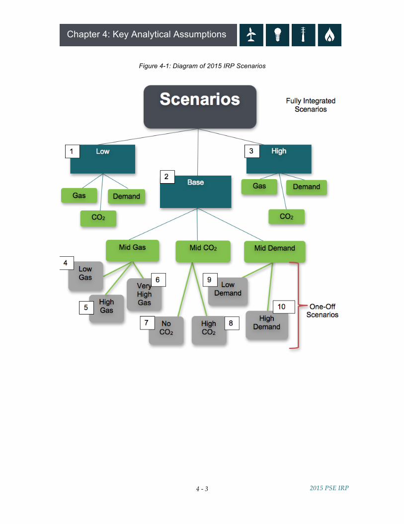
OVERVIEW Scenarios and sensitivities play a key role in the deterministic phase of the IRP analysis. Scenarios allow us to test the impact of different sets of economic conditions on resource strategy. Using deterministic optimization analysis, we identify the least-cost portfolio of demand- and supply-side resources that will meet need, given the set of static assumptions that define the scenario. For this IRP, PSE developed 10 scenarios.

• THREE FULLY INTEGRATED SCENARIOS – Low, Base and High – reflect different sets of assumptions for each of three fundamental economic inputs: customer demand, natural gas prices and CO2 prices.

• SEVEN ONE-OFF SCENARIOS start with Base Scenario assumptions and change just one of those three variables to isolate its effect on PSE’s resource plans, costs and emissions.

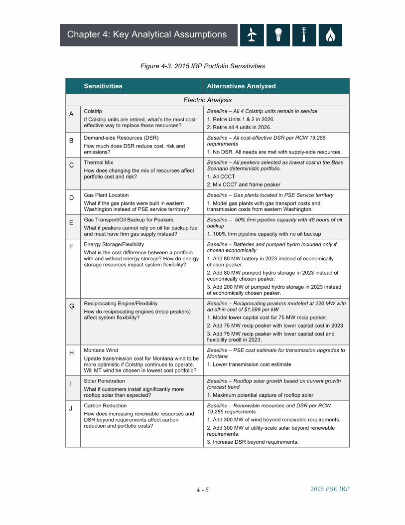
To complete the scenarios, we create wholesale power price assumptions for each one using an Aurora analysis described later in this chapter. Figure 4-1 illustrates the relationship between the fully integrated and one-off scenarios. Sensitivities start with baseline portfolio assumptions and change a single resource variable. This makes it possible to examine the cost-effectiveness of a given resource, the value it brings to the portfolio, and explore how PSE might need to respond to unexpected changes in resource availability. The sensitivities are summarized in Figure 4-3.

4 - 3


2015 PSE IRP

Figure 4-1: Diagram of 2015 IRP Scenarios

4 - 4


2015 PSE IRP

Figure 4-2: 2015 IRP Scenarios

Scenario Name Gas Price CO2 Price Demand

1 Low Scenario Low None Low

2 Base Scenario Mid Mid Mid

3 High Scenario High High High

4 Base + Low Gas Price Low Mid Mid

5 Base + High Gas Price High Mid Mid

6 Base + Very High Gas Price Very High Mid Mid

7 Base + No CO2 Mid None Mid

8 Base + High CO2 Mid High Mid

9 Base + Low Demand Mid Mid Low

10 Base + High Demand Mid Mid High

4 - 5


2015 PSE IRP

Figure 4-3: 2015 IRP Portfolio Sensitivities

Sensitivities Alternatives Analyzed

Electric Analysis

A Colstrip If Colstrip units are retired, what’s the most cost-effective way to replace those resources?

Baseline – All 4 Colstrip units remain in service 1. Retire Units 1 & 2 in 2026. 2. Retire all 4 units in 2026.

B Demand-side Resources (DSR) How much does DSR reduce cost, risk and emissions?

Baseline – All cost-effective DSR per RCW 19.285 requirements 1. No DSR. All needs are met with supply-side resources.

C Thermal Mix How does changing the mix of resources affect portfolio cost and risk?

Baseline – All peakers selected as lowest cost in the Base Scenario deterministic portfolio. 1. All CCCT 2. Mix CCCT and frame peaker

D Gas Plant Location What if the gas plants were built in eastern Washington instead of PSE service territory?

Baseline – Gas plants located in PSE Service territory 1. Model gas plants with gas transport costs and transmission costs from eastern Washington.

E Gas Transport/Oil Backup for Peakers What if peakers cannot rely on oil for backup fuel and must have firm gas supply instead?

Baseline – 50% firm pipeline capacity with 48 hours of oil backup 1. 100% firm pipeline capacity with no oil backup

F Energy Storage/Flexibility What is the cost difference between a portfolio with and without energy storage? How do energy storage resources impact system flexibility?

Baseline – Batteries and pumped hydro included only if chosen economically 1. Add 80 MW battery in 2023 instead of economically chosen peaker. 2. Add 80 MW pumped hydro storage in 2023 instead of economically chosen peaker. 3. Add 200 MW of pumped hydro storage in 2023 instead of economically chosen peaker.

G Reciprocating Engine/Flexibility How do reciprocating engines (recip peakers) affect system flexibility?

Baseline – Reciprocating peakers modeled at 220 MW with an all-in cost of $1,599 per kW 1. Model lower capital cost for 75 MW recip peaker. 2. Add 75 MW recip peaker with lower capital cost in 2023. 3. Add 75 MW recip peaker with lower capital cost and flexibility credit in 2023.

H Montana Wind Update transmission cost for Montana wind to be more optimistic if Colstrip continues to operate. Will MT wind be chosen in lowest cost portfolio?

Baseline – PSE cost estimate for transmission upgrades to Montana 1. Lower transmission cost estimate

I Solar Penetration What if customers install significantly more rooftop solar than expected?

Baseline – Rooftop solar growth based on current growth forecast trend 1. Maximum potential capture of rooftop solar

J Carbon Reduction How does increasing renewable resources and DSR beyond requirements affect carbon reduction and portfolio costs?

Baseline – Renewable resources and DSR per RCW 19.285 requirements 1. Add 300 MW of wind beyond renewable requirements. 2. Add 300 MW of utility-scale solar beyond renewable requirements. 3. Increase DSR beyond requirements.

4 - 6


2015 PSE IRP

Sensitivities Alternatives Analyzed

Natural Gas Analysis

A Alternate Discount Rate Test cost-effective amount of DSR using alternate discount rate to model the value of DSR over time.

Baseline – Use PSE WACC of 7.77% 1. Use alternate discount rate of 4.93%.

B Pipeline Timing Does smoothing out the pipeline capacity expansion change the lowest cost portfolio?

Baseline – Allow pipeline capacity expansion to be built in 2026 and 2030 2. Allow pipeline capacity expansion to be built every year starting in 2026

4 - 7


2015 PSE IRP

KEY INPUTS

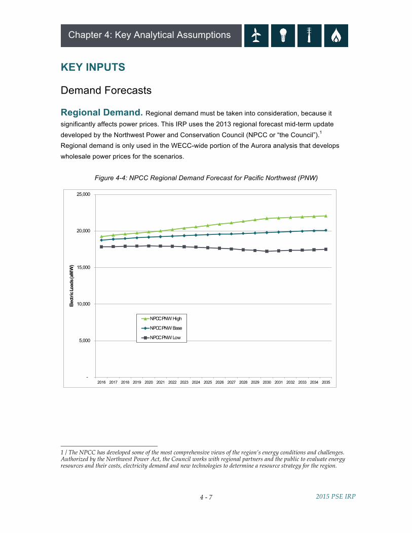
Demand Forecasts Regional Demand. Regional demand must be taken into consideration, because it significantly affects power prices. This IRP uses the 2013 regional forecast mid-term update developed by the Northwest Power and Conservation Council (NPCC or “the Council”).1

Regional demand is only used in the WECC-wide portion of the Aurora analysis that develops wholesale power prices for the scenarios.

Figure 4-4: NPCC Regional Demand Forecast for Pacific Northwest (PNW)

1 / The NPCC has developed some of the most comprehensive views of the region’s energy conditions and challenges. Authorized by the Northwest Power Act, the Council works with regional partners and the public to evaluate energy resources and their costs, electricity demand and new technologies to determine a resource strategy for the region.

-

5,000

10,000

15,000

20,000

25,000

2016 2017 2018 2019 2020 2021 2022 2023 2024 2025 2026 2027 2028 2029 2030 2031 2032 2033 2034 2035

Elec

tric

Load

s (aM

W)

NPCC PNW High

NPCC PNW Base

NPCC PNW Low

4 - 8


2015 PSE IRP

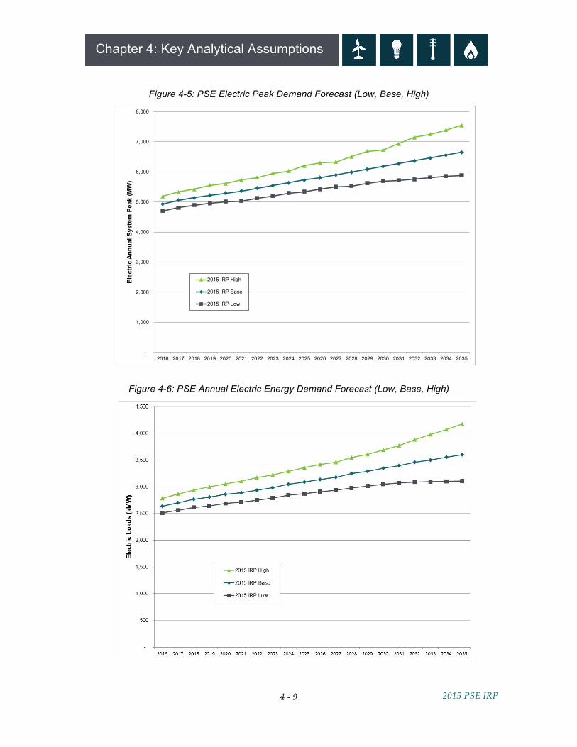
PSE Demand. PSE customer demand is the single most important input assumption to the IRP portfolio analysis. The demand forecast is discussed in detail in Chapter 5, and the analytical models used to develop it are explained in Appendix F, Demand Forecasting Models. For long-range planning, customer demand is expressed as if it were evenly distributed throughout PSE’s service territory, but in reality demand grows faster in some parts of the territory and slower in others.

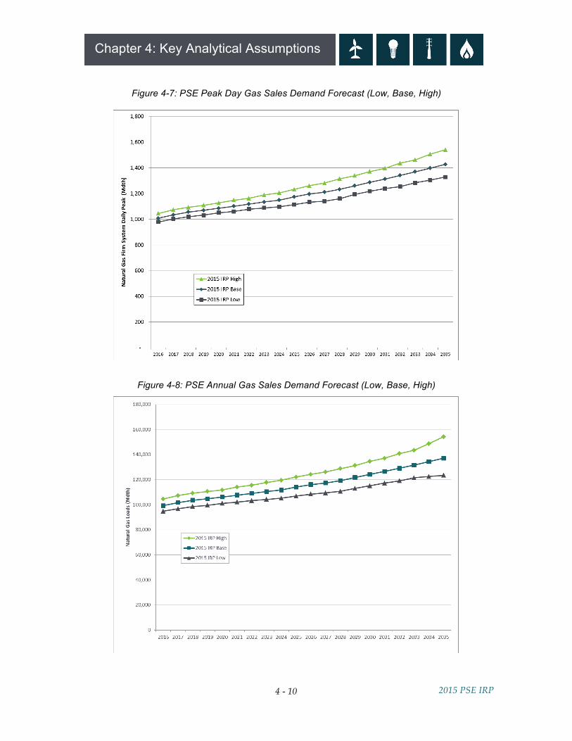
The three demand forecasts used in this IRP analysis represent estimates of energy sales, customer counts and peak demand over a 20-year period. Significant inputs include information about regional and national economic growth, demographic changes, weather, prices, seasonality and other customer usage and behavior factors. Known large load additions or deletions are also included. The 2015 IRP BASE DEMAND FORECAST is based on 2014 macroeconomic conditions such as population growth and unemployment. It is used in the 2015 IRP Base Scenario. The 2015 IRP LOW DEMAND FORECAST represents a pessimistic view of the macroeconomic variables modeled in the base forecast. It creates lower demand on the system and is used in the 2015 IRP Low Scenario. The 2015 IRP HIGH DEMAND FORECAST is a more optimistic view of the base forecast. It creates a higher demand on the system and is used in the 2015 IRP High Scenario. The graphs below show the peak demand and annual energy demand forecasts for electric service and gas sales. Both the electric and gas demand forecasts include sales (delivered load) plus system losses. The electric peak demand forecast is for a one-hour temperature of 23° Fahrenheit at SeaTac airport; this is considered the 1-in-2 peak. The gas sales peak demand forecast is for a one-day temperature of 13° Fahrenheit at SeaTac airport; this is considered the 1-in-20 peak.

Why don’t demand forecasts in rate cases and acquisition discussions match the IRP forecast? The IRP analysis takes 12 to 18 months to complete. Demand forecasts are so central to the analysis that they are one of the first inputs we need to develop. By the time the IRP is completed, PSE will have updated its demand forecast. The range of possibilities in the IRP forecast is sufficient for long-term planning purposes, but we will always present the most current forecast for rate cases or when making acquisition decisions.

4 - 9


2015 PSE IRP

Figure 4-5: PSE Electric Peak Demand Forecast (Low, Base, High)

Figure 4-6: PSE Annual Electric Energy Demand Forecast (Low, Base, High)

-

1,000

2,000

3,000

4,000

5,000

6,000

7,000

8,000

2016 2017 2018 2019 2020 2021 2022 2023 2024 2025 2026 2027 2028 2029 2030 2031 2032 2033 2034 2035

Elec

tric

Ann

ual S

yste

m P

eak

(MW

)

2015 IRP High

2015 IRP Base

2015 IRP Low

4 - 10


2015 PSE IRP

Figure 4-7: PSE Peak Day Gas Sales Demand Forecast (Low, Base, High)

Figure 4-8: PSE Annual Gas Sales Demand Forecast (Low, Base, High)

4 - 11


2015 PSE IRP

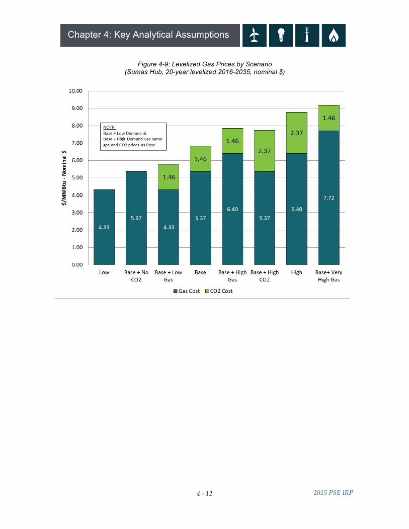
Gas Prices For gas price assumptions, PSE uses a combination of forward market prices, fundamental forecasts acquired in November 2014 from Wood Mackenzie, and forecasts developed by the NPCC. Wood MacKenzie is a well-known macroeconomic and energy forecasting consultancy whose gas market analysis includes regional, North American and international factors, as well as Canadian markets and liquefied natural gas (LNG) exports. The NPCC focuses on energy planning issues in the Northwest region. Four gas price forecasts are used in the scenario analysis: LOW GAS PRICES. These reflect Wood Mackenzie’s long-term low price forecast for 2016-2035. MID GAS PRICES. From 2016-2019, this IRP uses the three-month average of forward marks for the period ending November 14, 2014. Forward marks reflect the price of gas being purchased at a given point in time for future delivery. Beyond 2019, this IRP uses Wood Mackenzie long-run, fundamentals-based gas price forecasts. The Base Scenario uses this forecast. HIGH GAS PRICES. These reflect Wood Mackenzie’s long-term high price forecast for 2016-2035. VERY HIGH GAS PRICES. This forecast reflects the NPCC high gas price forecast developed in July 2014. Figure 4-9 below illustrates the range of 20-year levelized gas prices and associated CO2 costs used in this IRP analysis.

4 - 12


2015 PSE IRP

Figure 4-9: Levelized Gas Prices by Scenario (Sumas Hub, 20-year levelized 2016-2035, nominal $)

4 - 13


2015 PSE IRP

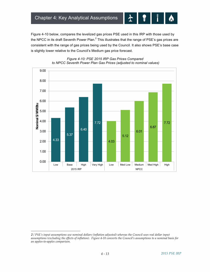
Figure 4-10 below, compares the levelized gas prices PSE used in this IRP with those used by the NPCC in its draft Seventh Power Plan.2 This illustrates that the range of PSE’s gas prices are consistent with the range of gas prices being used by the Council. It also shows PSE’s base case is slightly lower relative to the Council’s Medium gas price forecast.

Figure 4-10: PSE 2015 IRP Gas Prices Compared to NPCC Seventh Power Plan Gas Prices (adjusted to nominal values)

2 / PSE’s input assumptions use nominal dollars (inflation adjusted) whereas the Council uses real dollar input assumptions (excluding the effects of inflation). Figure 4-10 converts the Council’s assumptions to a nominal basis for an apples-to-apples comparison.

4.335.37

6.40

7.72

4.035.12

6.016.87

7.72

0.00

1.00

2.00

3.00

4.00

5.00

6.00

7.00

8.00

9.00

Low Base High Very High Low Med Low Medium Med High High

2015 IRP NPCC

Nom

inal

$/M

MBt

u

4 - 14


2015 PSE IRP

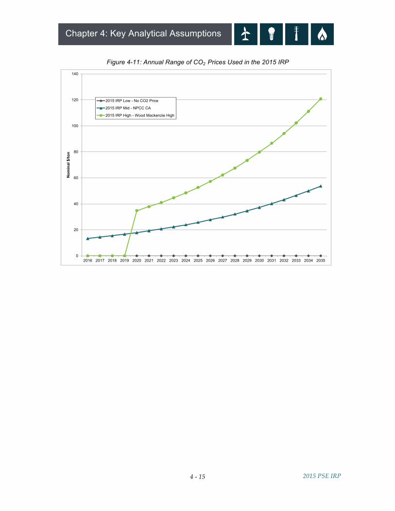
CO2 Prices To model uncertainty around CO2 prices, PSE developed the following estimates as inputs. These estimates reflect the potential for CO2 price regulation and how that might affect resource decisions, rather than incorporating the societal cost of carbon emissions as an externality. A table showing the annual CO2 prices modeled can be found in Appendix N, Electric Analysis. NO FEDERAL CO2 PRICE. $0 PER TON. The lowest CO2 price used in the 2015 IRP assumes no federal CO2 price, but does include an NPCC forecast of California CO2 prices based on the California Global Warming Solutions Act of 2006 (AB32).3 This CO2 price is applied to power plants located in California. MID CO2 PRICE. $13 PER TON IN 2016 TO $54 PER TON IN 2035. This estimate is based on NPCC’s estimated CO2 price for California AB32 and is applied as a federal CO2 price to all resources. HIGH CO2 PRICE. $35 PER TON IN 2020 TO $120 PER TON IN 2035. This estimate of federal CO2 price comes from the Wood Mackenzie high gas price forecast; California CO2 price are increased to match federal CO2 price.

3 / See Appendix C, Environmental Matters, for more details on the California Global Warming Solutions Act.

Why model potential carbon price regulation instead of the societal cost of carbon? By rule the IRP focuses on the costs and benefits that will be experienced by the utility and its customers. Costs and benefits outside of this construct are called externalities. The societal cost of carbon is a difficult externality to model for many reasons. Reducing carbon emissions may benefit society as a whole, but the population of our service territory is only 2.6 million (0.04 percent of the world’s population). To reflect the externality impact of carbon reductions to PSE’s customers would require either a reasonable estimate of the economic impact on the Pacific Northwest region (which is not available) or prorating the societal benefits that will accrue to our customers only. This highlights the “Tragedy of the Commons” problem associated with climate change, and explains why internalizing these externalities in typical IRP analyses is not a substitute for federal-level carbon regulation policies.

4 - 15


2015 PSE IRP

Figure 4-11: Annual Range of CO2 Prices Used in the 2015 IRP

0

20

40

60

80

100

120

140

2016 2017 2018 2019 2020 2021 2022 2023 2024 2025 2026 2027 2028 2029 2030 2031 2032 2033 2034 2035

Nom

inal

$/to

n

2015 IRP Low - No CO2 Price

2015 IRP Mid - NPCC CA

2015 IRP High - Wood Mackenzie High

4 - 16


2015 PSE IRP

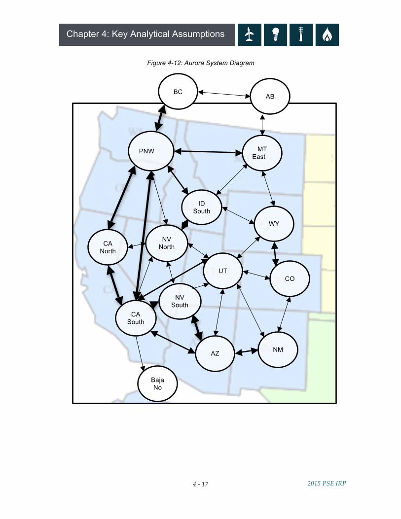
Developing Wholesale Power Prices A power price forecast is developed for each of the 10 scenarios modeled. In this context, “power price” does not mean the rate charged to customers, it means the price to PSE of purchasing (or selling) 1 megawatt (MW) of power on the wholesale market given the economic conditions that prevail in that scenario. This is an important input to the analysis, since market purchases make up a substantial portion of PSE’s resource portfolio. AURORAxmp is an hourly chronological price forecasting model based on market fundamentals. Creating wholesale power price assumptions requires performing two WECC-wide Aurora model runs for each of the 10 scenarios (Aurora is discussed in more detail in Appendix N, Electric Analysis). The first run identifies needed capacity expansion to meet regional loads. Aurora looks at loads and peak demand plus a planning margin, and then identifies the most economic resource(s) to add to make sure that all regions modeled are in balance. Results of the capacity expansion run are included in Appendix N, Electric Analysis. The second Aurora run produces hourly power prices. A full simulation across the entire WECC region simulates power prices in all 15 zones shown in Figure 4-12 below. The lines and arrows in the diagram indicate transmission links between zones. The heavier lines represent greater capacity to flow power from one zone to another.

4 - 17


2015 PSE IRP

Figure 4-12: Aurora System Diagram

PNW MT East

ID South

WY

CO

NM AZ

UT

NV South

NV North CA

North

CA South

BC AB

Baja No

4 - 18


2015 PSE IRP

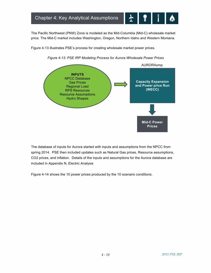
The Pacific Northwest (PNW) Zone is modeled as the Mid-Columbia (Mid-C) wholesale market price. The Mid-C market includes Washington, Oregon, Northern Idaho and Western Montana. Figure 4-13 illustrates PSE’s process for creating wholesale market power prices.

Figure 4-13: PSE IRP Modeling Process for Aurora Wholesale Power Prices

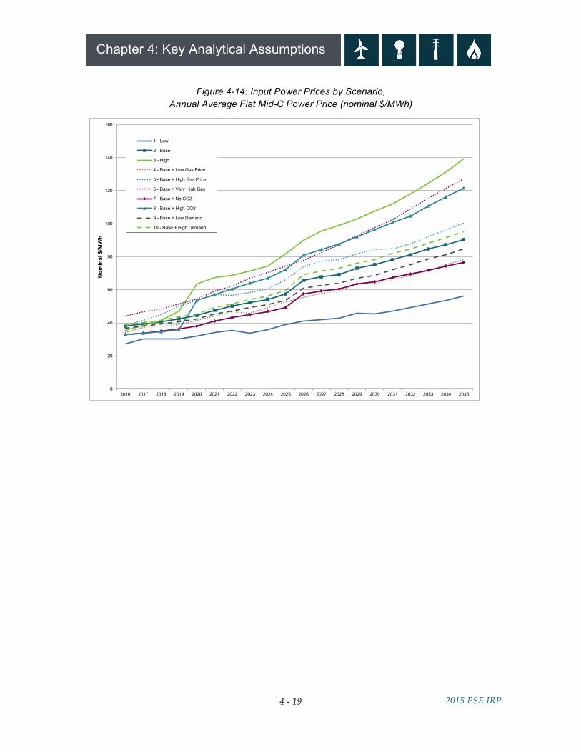
The database of inputs for Aurora started with inputs and assumptions from the NPCC from spring 2014. PSE then included updates such as Natural Gas prices, Resource assumptions, CO2 prices, and inflation. Details of the inputs and assumptions for the Aurora database are included in Appendix N, Electric Analysis Figure 4-14 shows the 10 power prices produced by the 10 scenario conditions.

INPUTS NPCC Database

Gas Prices Regional Load

RPS Resources Resource Assumptions

Hydro Shapes

Capacity Expansion and Power price Run

(WECC)

AURORAxmp

Mid-C Power Prices

4 - 19


2015 PSE IRP

Figure 4-14: Input Power Prices by Scenario, Annual Average Flat Mid-C Power Price (nominal $/MWh)

0

20

40

60

80

100

120

140

160

2016 2017 2018 2019 2020 2021 2022 2023 2024 2025 2026 2027 2028 2029 2030 2031 2032 2033 2034 2035

Nom

inal

$/M

Wh

1 - Low

2 - Base

3 - High

4 - Base + Low Gas Price

5 - Base + High Gas Price

6 - Base + Very High Gas

7 - Base + No CO2

8 - Base + High CO2

9 - Base + Low Demand

10 - Base + High Demand

4 - 20


2015 PSE IRP

SCENARIOS AND SENSITIVITES The scenarios developed for the IRP enable us to test portfolio costs and risks in a wide variety of possible future conditions using deterministic optimization analysis. Sensitivities enable us to isolate the effects of an individual variable on resource portfolios. The full range of scenarios is described first, followed by a description of the baseline assumptions that apply to all scenarios.

Fully Integrated Scenarios Three fully integrated scenarios model a complete range of key indicators: customer demand, natural gas prices and CO2 prices.4 1. Low Scenario

• This scenario models weaker long-term economic growth than the Base Scenario. Customer demand is lower in the region and in PSE’s service territory. The NPCC low growth rate is applied for the WECC region, and the 2015 IRP Low Demand Forecast is applied for PSE.

• Natural gas prices are lower due to lower energy demand; the Wood Mackenzie long-term low forecast is applied to natural gas prices.

• No federal CO2 price is applied, but California CO2 prices per AB32 are included. 2. Base Scenario

• The Base Scenario applies the NPCC 2013 regional demand forecast to the WECC region and the 2015 IRP Base Demand Forecast for PSE.

• Mid Gas Prices are applied, a combination of forward market prices and Wood Mackenzie’s fundamental long-term base forecast.

• Mid CO2 prices are modeled: $13 per ton in 2016 to $54 per ton in 2035, plus California CO2 prices per AB32.

3. High Scenario

• This scenario models more robust long-term economic growth, which produces higher customer demand. The NPCC high growth rate is applied for the WECC, and the 2015 IRP High Demand Forecast is applied for PSE.

• Natural gas prices are higher as a result of increased demand, so the high gas price assumptions are modeled (Wood Mackenzie long-term high forecast for 2016-2035).

• High CO2 prices are modeled: $35 per ton in 2020 to $120 per ton in 2035, plus California CO2 prices are increased to match federal CO2 prices.

4 / See Figures 4-1 and 4-2.

4 - 21


2015 PSE IRP

One-off Scenarios Seven one-off scenarios start with the Base Scenario and change just one of the three key conditions. 4. Base + Low Gas Price

This scenario models the impact of a weak long-term gas price by applying the Wood Mackenzie’s long-term low gas price forecast to Base Scenario assumptions.

5. Base + High Gas Price

This scenario models the impact of a higher long-term gas price by applying the Wood Mackenzie long-term high gas price forecast for 2016-2035 to Base Scenario assumptions.

6. Base + Very High Gas Price

This scenario models a future in which gas prices are extremely high; it applies the NPCC high gas price forecast to Base Scenario assumptions.

7. Base + No CO2 This scenario removes federal CO2 prices from Base Scenario assumptions, but retains a CO2 price for California.

8. Base + High CO2

This scenario models a future in which CO2 prices are high; it applies the high CO2 price estimate ($35 per ton in 2020 to $120 per ton in 2035) to Base Scenario assumptions.

9. Base + Low Demand

This scenario models low customer demand in the context of Base Scenario assumptions; it applies the 2015 IRP Low Demand Forecast.

10. Base + High Demand This scenario models high customer demand in the context of Base Scenario assumptions; it applies the 2015 IRP High Demand Forecast.

4 - 22


2015 PSE IRP

Baseline Scenario Assumptions – Electric Baseline scenario assumptions are constant in all scenarios and portfolios and do not change. Resource Assumptions. PSE modeled the following generic resources as potential portfolio additions in this IRP analysis. (See Appendix D, Electric Resources and Alternatives, for more detailed descriptions of the resources listed here.) Supply-side resources include the following. COMBINED-CYCLE COMBUSTION TURBINES (CCCTS). F-type, 1x1 engines with wet cooling towers are assumed to generate 335 MW plus 50 MW of duct firing, and are located in PSE’s service territory. SIMPLE-CYCLE COMBUSTION TURBINES (FRAME PEAKERS). F-type, wet-cooled turbines are assumed to generate 228 MW and are located in PSE’s service territory. Those modeled without oil backup were required to have firm gas supplies and storage. AERODERIVATIVE COMBUSTION TURBINES (AERO PEAKERS). The 2-turbine design with wet cooling is assumed to generate a total of 203 MW and to be located in PSE’s service territory. Those modeled without oil backup were required to have firm gas supplies and storage. RECIPROCATING ENGINES (RECIP PEAKERS). This 12-engine design (18 MW each) with wet cooling, is assumed to generate a total of 220 MW and to be located in PSE’s service territory. WIND. Wind was modeled in southeast Washington and central Montana. Washington wind is assumed to have a capacity factor of 34 percent. Montana wind is assumed to be located east of the continental divide and have a capacity factor of 41 percent. ENERGY STORAGE. Two energy storage technologies are modeled: batteries and pumped hydro. The generic battery resource is lithium-ion technology. Pumped hydro resources are generally large, on the order of 250 to 3,000 MW. This analysis assumes PSE would split the output of a pumped hydro storage project with other interested parties. SOLAR. Utility-scale solar PV is assumed to be located in central to southern Washington, use a fixed tilt system, and have a capacity factor of 20 percent.

“Peaker” is a term used to describe generators that can ramp up and down quickly in order to meet spikes in need.

4 - 23


2015 PSE IRP

Demand-side resources include the following. ENERGY EFFICIENCY MEASURES. This label is used for a wide variety of measures that result in a lower level of energy being used for doing the same amount of work. These often focus on retrofitting programs and new construction codes and standards and include measures like appliance upgrades, building envelope upgrades, heating and cooling systems and lighting changes. DEMAND-RESPONSE. Demand-response resources are comprised of flexible, price-responsive loads, which may be curtailed or interrupted during system emergencies or when wholesale market prices exceed the utility’s supply cost. DISTRIBUTED GENERATION. Distributed generation refers to small-scale electricity generators (like rooftop solar panels) located close to the source of the customer’s load. DISTRIBUTION EFFICIENCY. Voltage reduction and phase balancing. Voltage reduction is the practice of reducing the voltage on distribution circuits to reduce energy consumption. Phase balancing eliminates total current flow losses that can reduce energy loss. GENERATION EFFICIENCY. Energy efficiency improvements at PSE generating plant facilities. CODES AND STANDARDS. No-cost energy efficiency measures that work their way to the market via new efficiency standards that originate from federal and state codes and standards. For detailed information on demand-side resource assumptions, see Appendix J, Demand-side Resources.

4 - 24


2015 PSE IRP

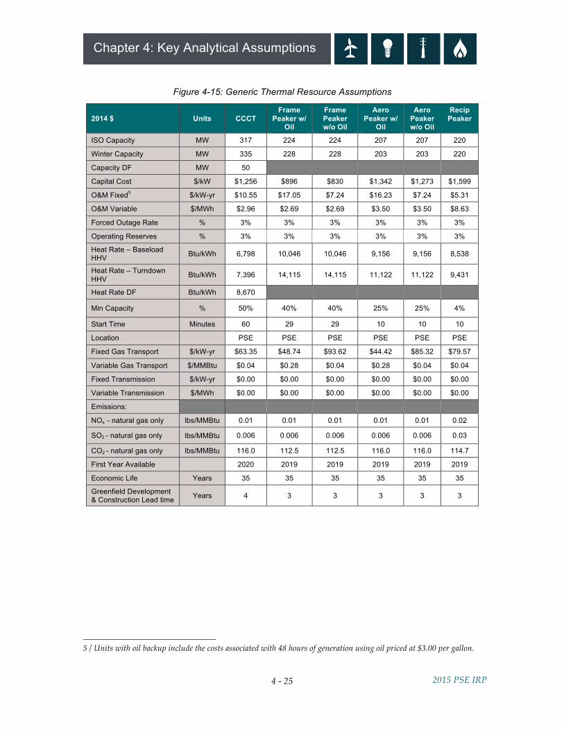
Resource Cost Assumptions. The estimated cost of generic natural gas resources is based on a May 2014 study by Black and Veatch done on behalf of PSE. Renewable resource costs are based on research for estimates in the region and on PSE’s experience in the market. The cost curves applied to both of these for the 20-year study period come from the Energy Information Administration (EIA) Annual Energy Outlook (AEO). New equipment costs are assumed to decrease over time. Appendix D, Electric Resources and Alternatives, contains a more detailed description of these assumptions. In general, cost assumptions represent the “all-in” cost to deliver a resource to customers; this includes plant, siting and financing costs. PSE’s activity in the resource acquisition market during the past ten years informs resource cost assumptions, and our extensive discussions with developers, vendors of key project components and firms that provide engineering, procurement and construction services lead us to believe the estimates used here are appropriate and reasonable.

• Figure 4-15 summarizes generic thermal resource assumptions. • Figure 4-16 summarizes gas transport costs for CCCTs and peakers with and without oil

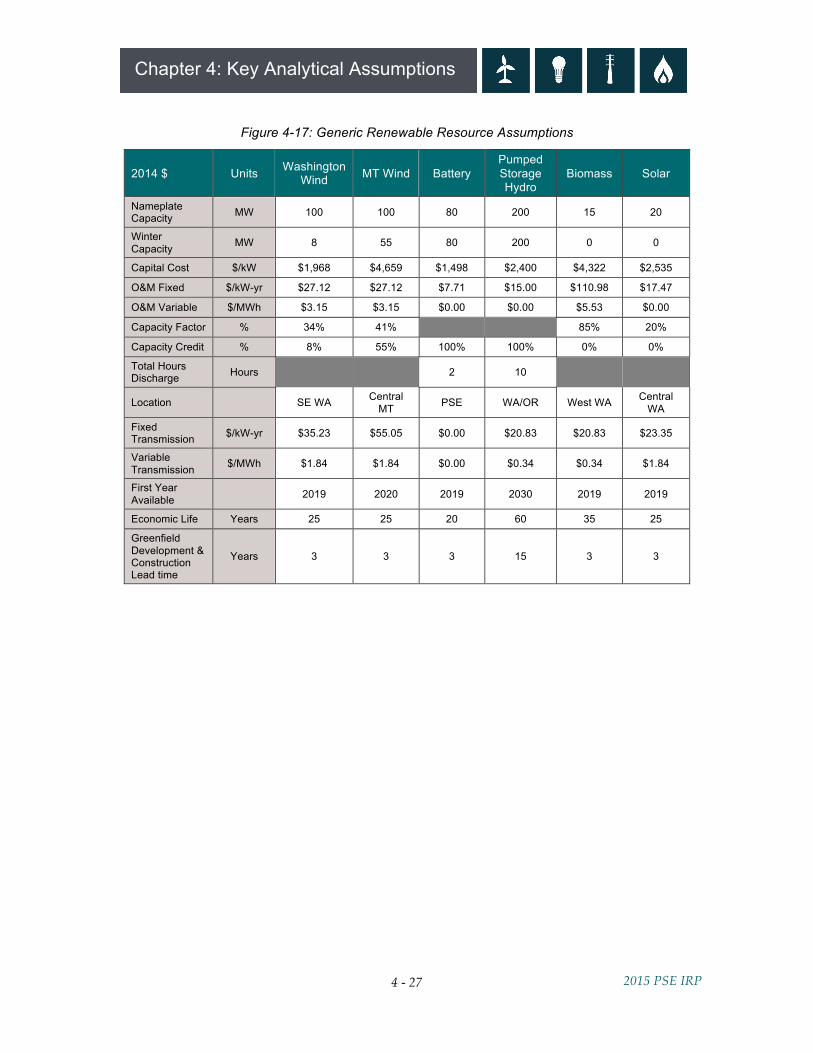
backup. • Figure 4-17 summarizes generic renewable resource assumptions. • Figure 4-18 displays the monthly capacity factor for Washington wind, Montana wind and

Washington solar. • Figure 4-19 summarizes annual capital cost by vintage year for supply-side resources,

batteries and pumped hydro storage.

4 - 25


2015 PSE IRP

Figure 4-15: Generic Thermal Resource Assumptions

2014 $ Units CCCT Frame

Peaker w/ Oil

Frame Peaker w/o Oil

Aero Peaker w/

Oil

Aero Peaker w/o Oil

Recip Peaker

ISO Capacity MW 317 224 224 207 207 220

Winter Capacity MW 335 228 228 203 203 220

Capacity DF MW 50

Capital Cost $/kW $1,256 $896 $830 $1,342 $1,273 $1,599

O&M Fixed5 $/kW-yr $10.55 $17.05 $7.24 $16.23 $7.24 $5.31

O&M Variable $/MWh $2.96 $2.69 $2.69 $3.50 $3.50 $8.63

Forced Outage Rate % 3% 3% 3% 3% 3% 3%

Operating Reserves % 3% 3% 3% 3% 3% 3%

Heat Rate – Baseload HHV Btu/kWh 6,798 10,046 10,046 9,156 9,156 8,538

Heat Rate – Turndown HHV Btu/kWh 7,396 14,115 14,115 11,122 11,122 9,431

Heat Rate DF Btu/kWh 8,670

Min Capacity % 50% 40% 40% 25% 25% 4%

Start Time Minutes 60 29 29 10 10 10

Location PSE PSE PSE PSE PSE PSE

Fixed Gas Transport $/kW-yr $63.35 $48.74 $93.62 $44.42 $85.32 $79.57

Variable Gas Transport $/MMBtu $0.04 $0.28 $0.04 $0.28 $0.04 $0.04

Fixed Transmission $/kW-yr $0.00 $0.00 $0.00 $0.00 $0.00 $0.00

Variable Transmission $/MWh $0.00 $0.00 $0.00 $0.00 $0.00 $0.00

Emissions:

NOx - natural gas only lbs/MMBtu 0.01 0.01 0.01 0.01 0.01 0.02

SO2 - natural gas only lbs/MMBtu 0.006 0.006 0.006 0.006 0.006 0.03

CO2 - natural gas only lbs/MMBtu 116.0 112.5 112.5 116.0 116.0 114.7

First Year Available 2020 2019 2019 2019 2019 2019

Economic Life Years 35 35 35 35 35 35

Greenfield Development & Construction Lead time Years 4 3 3 3 3 3

5 / Units with oil backup include the costs associated with 48 hours of generation using oil priced at $3.00 per gallon.

4 - 26


2015 PSE IRP

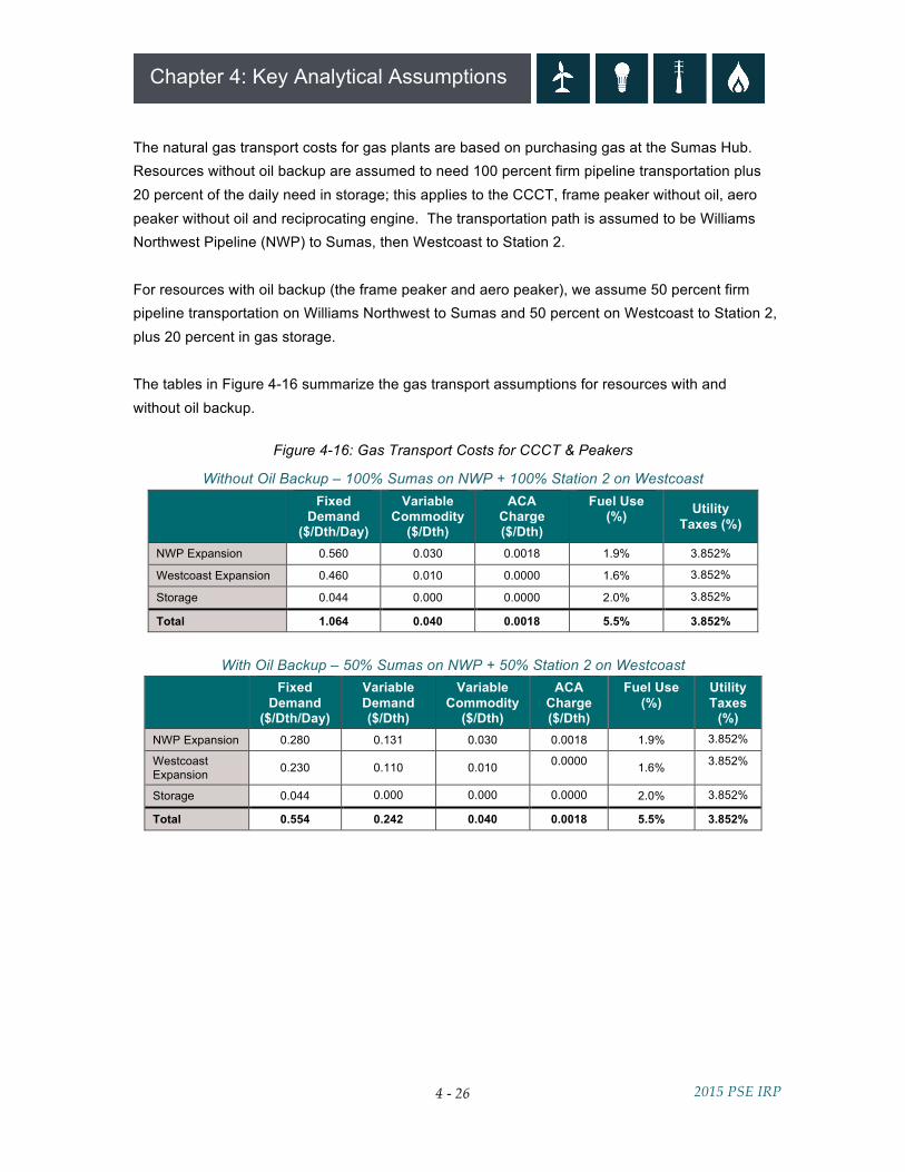
The natural gas transport costs for gas plants are based on purchasing gas at the Sumas Hub. Resources without oil backup are assumed to need 100 percent firm pipeline transportation plus 20 percent of the daily need in storage; this applies to the CCCT, frame peaker without oil, aero peaker without oil and reciprocating engine. The transportation path is assumed to be Williams Northwest Pipeline (NWP) to Sumas, then Westcoast to Station 2. For resources with oil backup (the frame peaker and aero peaker), we assume 50 percent firm pipeline transportation on Williams Northwest to Sumas and 50 percent on Westcoast to Station 2, plus 20 percent in gas storage. The tables in Figure 4-16 summarize the gas transport assumptions for resources with and without oil backup.

Figure 4-16: Gas Transport Costs for CCCT & Peakers

Without Oil Backup – 100% Sumas on NWP + 100% Station 2 on Westcoast

Fixed

Demand ($/Dth/Day)

Variable Commodity

($/Dth)

ACA Charge ($/Dth)

Fuel Use (%) Utility

Taxes (%)

NWP Expansion 0.560 0.030 0.0018 1.9% 3.852%

Westcoast Expansion 0.460 0.010 0.0000 1.6% 3.852%

Storage 0.044 0.000 0.0000 2.0% 3.852%

Total 1.064 0.040 0.0018 5.5% 3.852%

With Oil Backup – 50% Sumas on NWP + 50% Station 2 on Westcoast

Fixed

Demand ($/Dth/Day)

Variable Demand ($/Dth)

Variable Commodity

($/Dth)

ACA Charge ($/Dth)

Fuel Use (%)

Utility Taxes

(%) NWP Expansion 0.280 0.131 0.030 0.0018 1.9% 3.852%

Westcoast Expansion 0.230 0.110 0.010 0.0000 1.6% 3.852%

Storage 0.044 0.000 0.000 0.0000 2.0% 3.852%

Total 0.554 0.242 0.040 0.0018 5.5% 3.852%

4 - 27


2015 PSE IRP

Figure 4-17: Generic Renewable Resource Assumptions

2014 $ Units Washington Wind MT Wind Battery

Pumped Storage Hydro

Biomass Solar

Nameplate Capacity MW 100 100 80 200 15 20

Winter Capacity MW 8 55 80 200 0 0

Capital Cost $/kW $1,968 $4,659 $1,498 $2,400 $4,322 $2,535

O&M Fixed $/kW-yr $27.12 $27.12 $7.71 $15.00 $110.98 $17.47

O&M Variable $/MWh $3.15 $3.15 $0.00 $0.00 $5.53 $0.00

Capacity Factor % 34% 41% 85% 20%

Capacity Credit % 8% 55% 100% 100% 0% 0%

Total Hours Discharge Hours 2 10

Location SE WA Central MT PSE WA/OR West WA Central

WA

Fixed Transmission $/kW-yr $35.23 $55.05 $0.00 $20.83 $20.83 $23.35

Variable Transmission $/MWh $1.84 $1.84 $0.00 $0.34 $0.34 $1.84

First Year Available 2019 2020 2019 2030 2019 2019

Economic Life Years 25 25 20 60 35 25

Greenfield Development & Construction Lead time

Years 3 3 3 15 3 3

4 - 28


2015 PSE IRP

Figure 4-18 displays the monthly capacity factor for Washington wind, Montana wind, and Washington solar.

Figure 4-18: Capacity Factor for Wind and Solar

0%

10%

20%

30%

40%

50%

60%

70%

Jan Feb Mar Apr May Jun Jul Aug Sep Oct Nov Dec

WA Wind

MT Wind

Solar

MT Wind Annual Average CF

WA Wind Annual Average CF

Solar Annual Average CF

4 - 29


2015 PSE IRP

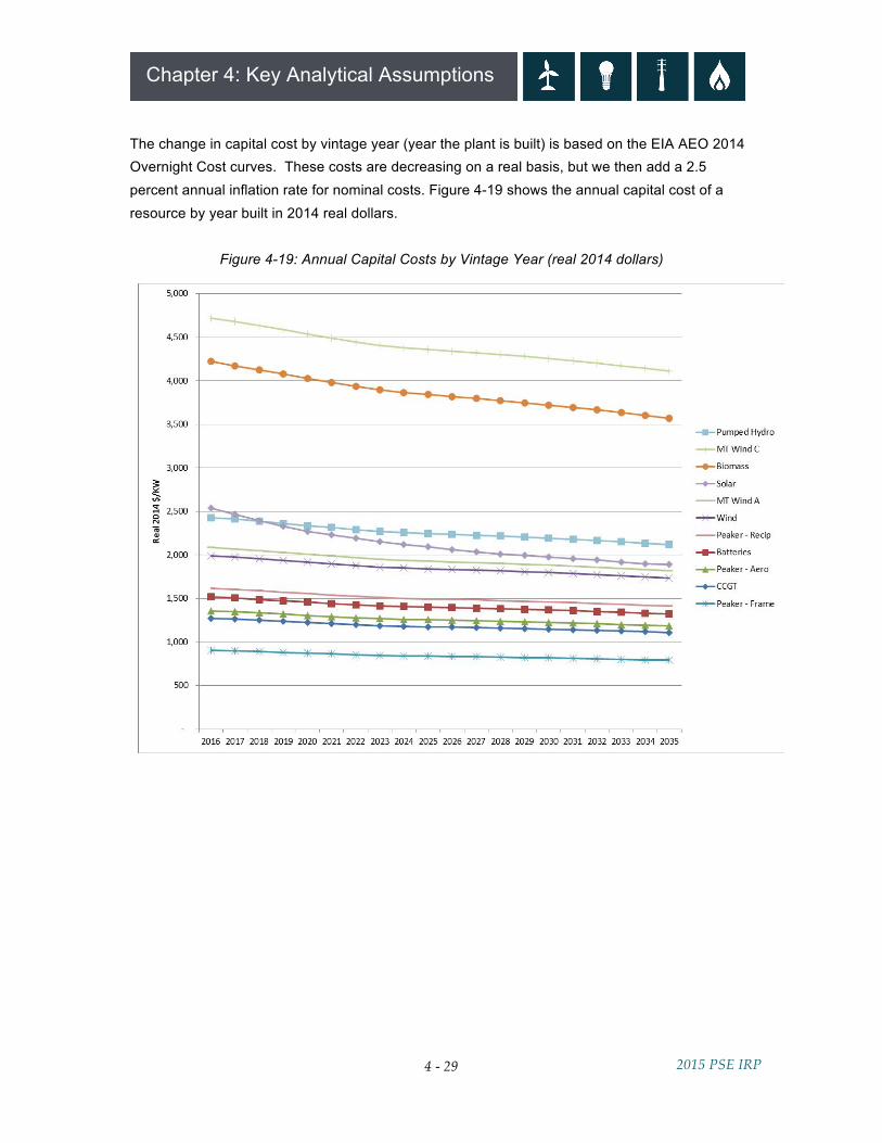
The change in capital cost by vintage year (year the plant is built) is based on the EIA AEO 2014 Overnight Cost curves. These costs are decreasing on a real basis, but we then add a 2.5 percent annual inflation rate for nominal costs. Figure 4-19 shows the annual capital cost of a resource by year built in 2014 real dollars.

Figure 4-19: Annual Capital Costs by Vintage Year (real 2014 dollars)

4 - 30


2015 PSE IRP

Heat Rates. PSE applies the improvements in new plant heat rates as estimated by the EIA in the AEO Base Case Scenario. New equipment heat rates are expected to improve slightly over time, as they have in the past. PSE also applies a 2 percent increase to the heat rates to account for the average degradation over the life of the plant. Federal Subsidies. Three federal subsidies reduced renewable resource costs in the U.S. during the most recent expansion of the renewable resource industry; however, these subsidies have now expired, and there is no momentum for renewal at this time. Since PSE has no near-term need for more renewable resources, this IRP does not include any additional resources to which such subsidies would apply if available. Renewable Portfolio Standards. Renewable portfolio standards (RPS) currently exist in 29 states and the District of Columbia, including most of the states in the WECC and British Columbia. They affect PSE because they increase competition for development of renewable resources. Each state and territory defines renewable energy sources differently, sets different timetables for implementation, and establishes different requirements for the percentage of load that must be supplied by renewable resources. To model these varying laws, PSE identifies the applicable load for each state in the model and the renewable benchmarks of each state’s RPS e.g. 3 percent in 2015, then 15 percent in 2020 for Washington State. Then we apply these requirements to each state’s load. No retirement of existing WECC renewable resources is assumed, which may underestimate the number of new resources that need to be constructed. After existing and "proposed" renewable energy resources are accounted for, "new" renewable energy resources are matched to the load to meet the applicable RPS. Following an internal and external review for reasonableness, these resources are created in the AURORA database. Technologies included wind, solar, biomass and geothermal. PSE used the same methodology as the NPCC to identify potential production by states. Production varies considerably depending on local conditions, e.g. Arizona has little wind potential but great solar potential. Appendix C, Environmental Matters, includes a table that identifies renewable portfolio standards for the states in the WECC.

4 - 31


2015 PSE IRP

Build and Retirement Constraints. Absent constraints, the AURORA model would identify coal as a least-cost resource and build new coal units in the WECC. To reflect current political and regulatory trends, PSE added constraints on coal technologies to the AURORA model. Specifically:

• No new coal builds are allowed in Washington. State law RCW 80.80 (Greenhouse Gases Emissions-Baseload Electric Generation Performance Standard) prohibits construction of new coal-fired generation within this state without carbon capture and sequestration.

• No new coal builds are allowed in any state in the WECC. In addition, all WECC coal plants must meet the National Ambient Air Quality Standards (NAAQS) and the Mercury and Air Toxics Standards (MATS).

• Any plant that has announced retirement is reflected in the database. • California power plants that would be shuttered by that state’s Once-through Cooling

regulations are retired. Further discussion of planned builds and retirements in WECC are discussed in Appendix N, Electric Analysis.

4 - 32


2015 PSE IRP

Electric Portfolio Sensitivity Reasoning Baseline assumptions are included in all portfolios. Sensitivities change one of those assumptions in order to isolate the effect of an individual variable on resource portfolios. Colstrip. Several proposed or recently enacted rules will affect the operation of the Colstrip plant in eastern Montana in coming years, so this IRP tests reducing reliance on Colstrip and eliminating it entirely.

BASELINE ASSUMPTION: All 4 units remain in service for the full planning period. Sensitivity 1 > Retire Units 1 & 2 in 2026. Sensitivity 2 > Retire all 4 units in 2026.

Demand-side Resources (DSR). This sensitivity looks at the effect of no additional DSR on portfolio cost and risk; all future needs are met with supply-side resources.

BASELINE ASSUMPTION: All cost-effective DSR per RPS requirements. Sensitivity 1 > Existing DSR measures stay in place, but all future needs are met with supply-side resources.

Thermal Mix. This sensitivity models different configurations of thermal resources.

BASELINE ASSUMPTION: Frame peakers were selected as the lowest-cost thermal resource addition in the deterministic analysis for the Base Scenario. Sensitivity 1 > This sensitivity models all CCCT plants instead of peakers. Sensitivity 2 > This sensitivity models a mix of frame peakers and CCCT plants.

Gas Plant Location. The purpose of this sensitivity is to model the cost differences between building a gas plant in PSE’s service territory on the western side of the Cascades versus building a plant in eastern Washington. The CCCT and peakers without oil backup located in western Washington have 100 percent firm pipeline transportation on NOVA, Foothills and GTN to AECO, with 20% storage. The western Washington located peakers with oil backup have 50 percent firm pipeline transportation on NOVA, Foothills and GTN to AECO, with 20% storage. All plants located in eastern Washington include firm Bonneville Power Administration transmission contract costs. A full discussion of costs and assumptions is located in Appendix D, Electric Resources and Alternatives.

4 - 33


2015 PSE IRP

BASELINE ASSUMPTION: Gas plants are located in PSE’s service territory with no added transmission cost and fuel transport to Sumas. Sensitivity 1 > Gas plants located in eastern Washington with firm transmission on BPA and fuel transport to AECO.

Gas Transport/Oil Backup for Peakers. The baseline assumption for peakers is that they have 50 percent of firm pipeline capacity and two days (48 hours) of oil backup, so they can rely on less expensive non-firm pipeline capacity for the remaining 50 percent of gas transport needs. The assumption is that 48 hours is enough time to find the needed pipeline capacity on the wholesale market. Available pipeline capacity is decreasing however, so the risk of being unable to acquire capacity when needed is increasing. This sensitivity tests the costs and risks associated with relying on more-expensive firm pipeline capacity for 100 percent of gas needs compared to 50 percent firm/50 percent non-firm capacity with 48 hours of oil backup.

BASELINE ASSUMPTION: Non-firm pipeline capacity with oil backup. Sensitivity 1 > Firm pipeline capacity with no oil backup.

Energy Storage/Flexibility. This sensitivity tests the effect of added batteries or pumped storage on the portfolio. Given the nature of storage resources, it is hard to compare them directly to a supply- or demand-side resource, so this test forces batteries and pumped storage into the portfolio so we can learn more about their impact on portfolio cost.

BASELINE ASSUMPTION: No contribution from pumped storage and batteries allowed to be added economically. Sensitivity 1 > 80 MW battery added into the portfolio in 2023 instead of economically chosen peaker. Sensitivity 2 > 80 MW pumped hydro storage added into the portfolio in 2023 instead of economically chosen peaker. Sensitivity 3 > 200 MW pumped hydro storage added into the portfolio in 2023 instead of economically chosen peaker.

4 - 34


2015 PSE IRP

Reciprocating Engines/Flexibility. This sensitivity looks at a lower-cost and smaller-sized configuration of reciprocating engine peakers. It also considers the flexibility benefit of reciprocating peakers on the portfolio.

BASELINE ASSUMPTION: Reciprocating peakers modeled at 220 MW with an all-in cost of $1,599 per kW. Sensitivity 1 > Recip peakers modeled at 75 MW with a lower updated all-in cost of $1,404 per kW Sensitivity 2 > Add 75 MW recip peakers to the portfolio in 2023 with the updated all-in cost of $1,404 per kW. Sensitivity 3 > Add 75 MW recip peaker in 2023 with the flexibility benefit from the 2013 IRP of $18.23 per kW-yr.6 This benefit was subtracted from the fixed operating and maintenance costs.

Montana Wind. The purpose of this sensitivity is to model a lower cost assumption for transmission from Montana. The current assumption models the Montana wind transmission and substation costs at $662 million. This includes line upgrades for the Judith Gap to Broadview line, an expanded Broadview substation, new Broadview to Garrison Line and an expanded Garrison substation. The assumption also includes a 6.7 percent line loss from Judith Gap to Garrison. A full discussion of the Montana wind assumptions can be found in Appendix D, Electric Resources and Alternatives.

BASELINE ASSUMPTION: Use PSE cost estimate for transmission upgrades to Montana. Sensitivity 1 > Include lower transmission cost estimate of $117 million for upgrades to Montana at the request of IRPAG stakeholder.

6 / See Appendix H, Operational Flexibility, for further information.

4 - 35


2015 PSE IRP

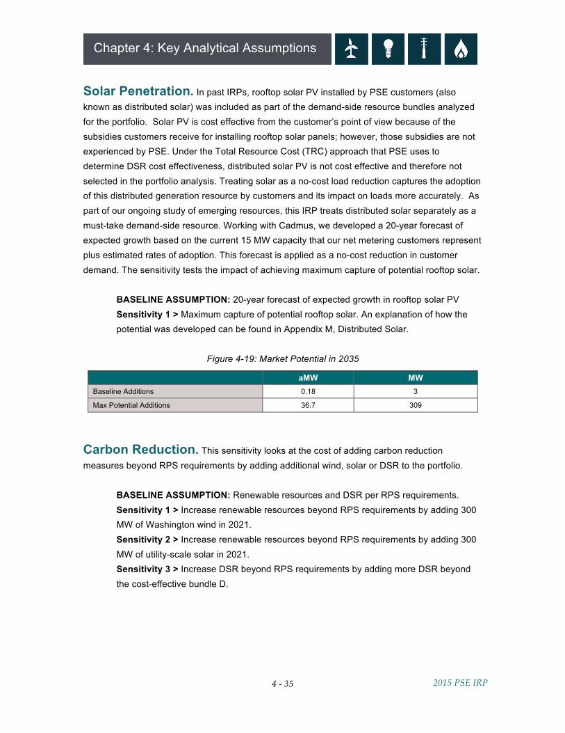
Solar Penetration. In past IRPs, rooftop solar PV installed by PSE customers (also known as distributed solar) was included as part of the demand-side resource bundles analyzed for the portfolio. Solar PV is cost effective from the customer’s point of view because of the subsidies customers receive for installing rooftop solar panels; however, those subsidies are not experienced by PSE. Under the Total Resource Cost (TRC) approach that PSE uses to determine DSR cost effectiveness, distributed solar PV is not cost effective and therefore not selected in the portfolio analysis. Treating solar as a no-cost load reduction captures the adoption of this distributed generation resource by customers and its impact on loads more accurately. As part of our ongoing study of emerging resources, this IRP treats distributed solar separately as a must-take demand-side resource. Working with Cadmus, we developed a 20-year forecast of expected growth based on the current 15 MW capacity that our net metering customers represent plus estimated rates of adoption. This forecast is applied as a no-cost reduction in customer demand. The sensitivity tests the impact of achieving maximum capture of potential rooftop solar.

BASELINE ASSUMPTION: 20-year forecast of expected growth in rooftop solar PV Sensitivity 1 > Maximum capture of potential rooftop solar. An explanation of how the potential was developed can be found in Appendix M, Distributed Solar.

Figure 4-19: Market Potential in 2035

aMW MW Baseline Additions 0.18 3

Max Potential Additions 36.7 309

Carbon Reduction. This sensitivity looks at the cost of adding carbon reduction measures beyond RPS requirements by adding additional wind, solar or DSR to the portfolio.

BASELINE ASSUMPTION: Renewable resources and DSR per RPS requirements. Sensitivity 1 > Increase renewable resources beyond RPS requirements by adding 300 MW of Washington wind in 2021. Sensitivity 2 > Increase renewable resources beyond RPS requirements by adding 300 MW of utility-scale solar in 2021. Sensitivity 3 > Increase DSR beyond RPS requirements by adding more DSR beyond the cost-effective bundle D.

4 - 36


2015 PSE IRP

Gas Sales Assumptions Resource Assumptions. Transportation and storage are key resources for natural gas utilities. Transporting gas from production areas or market hubs to PSE’s service area generally requires assembling a number of specific pipeline segments and/or gas storage alternatives. Purchases from specific market hubs are joined with various upstream and direct-connect pipeline alternatives and storage options to create combinations that have different costs and benefits. See Chapter 7, Gas Sales Analysis, for further information. In this IRP, eight alternatives were tested in the analyses.

1. Northern British Columbia (BC) gas at the Station 2 hub, delivered via Westcoast and Northwest Pipeline (NWP) expansions to PSE’s service area.

2. AECO gas delivered to PSE via existing or expanded capacity on NOVA and Foothills

pipelines, the prospective FORTIS BC Kingsvale-Oliver Reinforcement Project (KORP) and then on expanded NWP.

3. Delivery of AECO gas via NOVA, Foothills and GTN pipelines, with final delivery via a

prospective Cross Cascades pipeline with an expansion on NWP (N-MAX, Palomar/Blue Bridge).

4. Purchase gas directly at Malin (or transported from the Rockies hub on the Ruby Pipeline), transport by back-haul on the GTN pipeline and on a prospective Cross Cascades pipeline and then on an NWP expansion to PSE’s service area.

5. Develop an on-system LNG peaking resource to serve the needs of core gas customers

that can also serve additional markets, including transportation. 6. Acquire MIST Storage from Northwest Natural after an expansion of the Mist storage

facility. 7. Upgrade the existing Swarr LP-air facility.

8. Demand-side resources include energy efficiency measures and building codes and

standards.

4 - 37


2015 PSE IRP

Build Constraints. Gas expansions are done in multi-year blocks to reflect the reality of the acquisition process. There is inherent “lumpiness” in gas pipeline expansion, since expanding pipelines in small increments every year is not practical. Pipeline companies need minimum capacity commitments to make an expansion economically viable. Thus the model is constrained to evaluate pipeline expansions in four-year blocks: 2018, 2022, 2026 and 2030. Similarly, some resources have more flexibility. The Swarr LP gas peaking facility’s upgrade was made available in two-year blocks: the winter of 2016/2017 and again in 2018/2019. Gas Sales Sensitivities Alternate Discount Rate Sensitivity. When gas prices fell to historic lows in recent years, the costs that utilities incurred to achieve DSR conservation goals became much harder to justify. For example, $30 of investment in energy efficiency measures may produce only $20 of immediate benefit today. However, conservation measures continue to accrue value over time, so $20 of benefit today may be worth $50 ten years from now. To model the value of DSR over time, this sensitivity tests the impact of using an “alternate discount rate” to evaluate cost-effective conservation. The baseline assumption is to use the weighted average cost of capital (WACC) assigned to PSE via rate cases to evaluate DSR measures.

BASELINE ASSUMPTION: Use PSE current allowed WACC as the discount rate. Sensitivity 1 > Use alternate discount rate of 4.93% instead of the WACC discount rate.

Pipeline Timing Sensitivity. In its response to the 2013 IRP, the Washington Utilities and Transportation Commission made the following request: “In the next IRP, PSE should conduct a second run of its model once the appropriate blocks of pipeline capacity are selected, to assess whether early acquisition of pipeline blocks impacts the timing of the selection of other resources.” 7 This sensitivity examines that possibility.

BASELINE ASSUMPTION: Pipeline capacity expansions are built in 2022, 2026 and 2030. Sensitivity 1 > Pipeline capacity expansion is allowed every year starting in 2022.

7 / Attachment A, Washington Utilities and Transportation Commission Comments on Puget Sound Energy’s 2013 Integrated Resource Plan Dockets UE-120767 & UG-120768 Section IV, Natural Gas Resources, Page 10.

key analytical assumptions - puget sound … forecasts, ... key analytical assumptions 2015 pse irp...

Documents