KdVwaves, jumps, solitons & mascarets

P.-Y. LagreeCNRS & Sorbonne Universite (former UPMC Univ Paris 06), UMR 7190,Institut Jean Le Rond ∂’Alembert, Boıte 162, F-75005 Paris, Francepyl@ccr.jussieu.fr ; www.lmm.jussieu.fr/∼lagree15 novembre 2021http://www.lmm.jussieu.fr/~lagree/COURS/M2MHP/kdv.pdf

Resume

Free surface flows of water are clearly ubiquitous on Earth. As viscosity is small,the inviscid equations of water flow are presented. First, the case of small ampli-tude perturbations in small depth is presented, so linearized, this leads to the”d’Alembert equation” or ”wave equation”. Second, the case of small amplitudeperturbations in any depth is presented, this allows to explain the dispersive beha-vior of water waves. This is called ”Airy wave theory”. Third the ”shallow watertheory” is presented, this corresponds to significant perturbations of the heightof water, which is small compared to the length of the waves ; the equations arenon linear (”Saint Venant” equations). Then, if one considers in this latter fra-mework small amplitude waves, and the first correction due to depth, one mayhave a balance between ”non linearities” and ”dispersion”, or a balance between”steepening” and ”spreading”. This leads to the solitary wave solution of ”KdVEquation” : the ”soliton”. The KdV (Korteweg–de Vries) equation is presented asan application of multiple scale analysis.

1 Introduction

1.1 Observations of the soliton

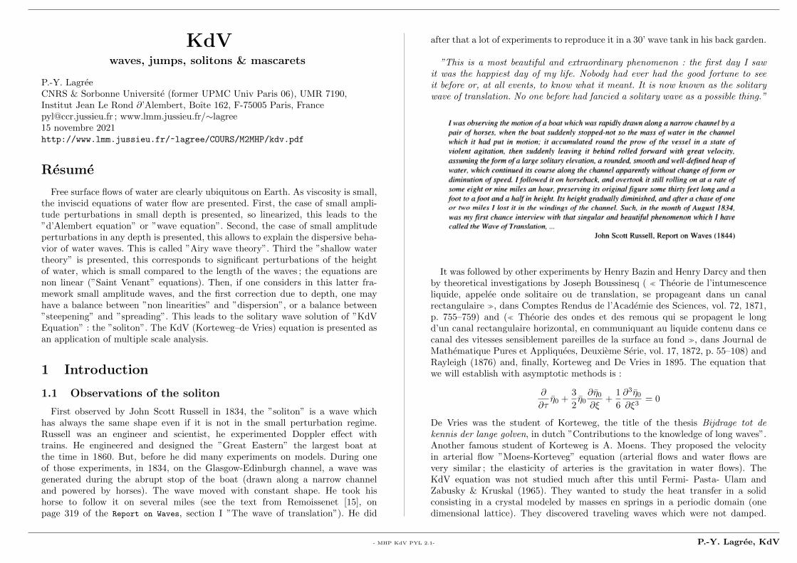
First observed by John Scott Russell in 1834, the ”soliton” is a wave whichhas always the same shape even if it is not in the small perturbation regime.Russell was an engineer and scientist, he experimented Doppler effect withtrains. He engineered and designed the ”Great Eastern” the largest boat atthe time in 1860. But, before he did many experiments on models. During oneof those experiments, in 1834, on the Glasgow-Edinburgh channel, a wave wasgenerated during the abrupt stop of the boat (drawn along a narrow channeland powered by horses). The wave moved with constant shape. He took hishorse to follow it on several miles (see the text from Remoissenet [15], onpage 319 of the Report on Waves, section I ”The wave of translation”). He did

after that a lot of experiments to reproduce it in a 30’ wave tank in his back garden.

”This is a most beautiful and extraordinary phenomenon : the first day I sawit was the happiest day of my life. Nobody had ever had the good fortune to seeit before or, at all events, to know what it meant. It is now known as the solitarywave of translation. No one before had fancied a solitary wave as a possible thing.”

It was followed by other experiments by Henry Bazin and Henry Darcy and thenby theoretical investigations by Joseph Boussinesq ( � Theorie de l’intumescenceliquide, appelee onde solitaire ou de translation, se propageant dans un canalrectangulaire �, dans Comptes Rendus de l’Academie des Sciences, vol. 72, 1871,p. 755–759) and (� Theorie des ondes et des remous qui se propagent le longd’un canal rectangulaire horizontal, en communiquant au liquide contenu dans cecanal des vitesses sensiblement pareilles de la surface au fond �, dans Journal deMathematique Pures et Appliquees, Deuxieme Serie, vol. 17, 1872, p. 55–108) andRayleigh (1876) and, finally, Korteweg and De Vries in 1895. The equation thatwe will establish with asymptotic methods is :

∂

∂τη0 +

3

2η0∂η0

∂ξ+

1

6

∂3η0

∂ξ3= 0

De Vries was the student of Korteweg, the title of the thesis Bijdrage tot dekennis der lange golven, in dutch ”Contributions to the knowledge of long waves”.Another famous student of Korteweg is A. Moens. They proposed the velocityin arterial flow ”Moens-Korteveg” equation (arterial flows and water flows arevery similar ; the elasticity of arteries is the gravitation in water flows). TheKdV equation was not studied much after this until Fermi- Pasta- Ulam andZabusky & Kruskal (1965). They wanted to study the heat transfer in a solidconsisting in a crystal modeled by masses en springs in a periodic domain (onedimensional lattice). They discovered traveling waves which were not damped.

- MHP KdV PYL 2.1- P.-Y. Lagree, KdV

They rediscoverd the soliton.

Figure 1 – The Soliton reproduced in 1995 on the very same placethan Scott Russell ’first’ observed a solitary wave on the Union Canalnear Edinburgh in 1834. (Photo from Nature v. 376, 3 Aug 1995, pg 373)http://www.ma.hw.ac.uk/solitons/press.html

See Dauxois, Newell [12], Remoissenet [15] and Maugin [14] for other historicaldetails and a view of the fields of application. The fields are very large, fromhydrodynamics, lattice waves, waves in electric lines, light waves in optic cablesetc. but as Feynman says : “Now, the next waves of interest, that are easily seen byeveryone and which are usually used as an example of waves in elementary courses,are water waves. As we shall soon see, they are the worst possible example, becausethey are in no respects like sound and light ; they have all the complications thatwaves can have.” Lectures on Physics, chapitre 51-4 “Ondes”.

1.2 Scope of the lecture : heuristical point of view, addingsmall dispersion

Waves in fluid are classical in mechanics of fluid courses. What we want to dohere is to restart from scratch this study with a uniform point of view in order torecover the ∂’Alembert Equation, the Saint Venant and the Airy Wave theory allin the same theoretical framework.

Figure 2 – The original sketches of Scott Russel. ”The great wave of transla-tion” http://www.ma.hw.ac.uk/∼chris/Scott-Russell/SR44.pdf. The wave may begenerated by a moving wall, top left or a falling weight top right, or opening agate. The final result is a unique wave which translates without change in shapeon very long distance.

For instance, the ∂’Alembert Equation, is heuristically proved as follows, we sup-pose a plug flow u(x, t), its acceleration is ρ∂u/∂t, the forces exerted are thepressure ones. Due to the elevation of the wave η (over the free level y = 0), thepressure is simply ρgη for hydrostatic reason (we will see that in more detailslater). Then

ρ∂u

∂t= −ρg ∂η

∂x,

The thickness of the fluid layer is h0, and η is smaller than h0, the other neededequation is the conservation of mass, as there is no v in the equations, changes of

- MHP KdV PYL 2.2- P.-Y. Lagree, KdV

the flux of u : ∂h0u∂x are compensated by the displacement of the interface :

∂η

∂t+∂h0u

∂x= 0.

At this point, to eliminate u, one needs the above mentioned hypothesis : the velo-city is almost constant across the layer (it looks like a plug flow, or in other words,the flow is irrotational). This gives the wave equation (∂’Alembert Equation) :

∂2η

∂t2− gh0

∂2η

∂x2= 0

with a celerity c0 =√gh0 and solution in f(x− c0t) + g(x+ c0t). To go further in

complexity, we can put some non linearities in these equation and suppose a plugflow (∂yu = 0). The total derivative is then ∂u

∂t + u∂u∂x , and flux will be (h0 + η)u,this will give the Saint Venant (Shallow Water) equations :

ρ∂u

∂t+ u

∂u

∂x= −ρg ∂η

∂x, and

∂η

∂t+∂hu

∂x= 0.

Or, we can imagine a linear small perturbation, with a flow which is no more aplug flow, but depends on x and y : u(x, y, t), this will give the famous dispersionrelation (again we will settle this again, see §3.3) :

ω2 = gk tanh(kh0).

for long waves, this equation gives again the ∂’Alembert one with c0 = ω/k =√gh0

Having in mind those equations describing the waves, then the solitary wavewill be presented as a mix of all this non linearity (η/h0 small) and dispersion,kh0 small. There are simple argument to settle at this point KdV such as :• from the wave equation the solution is u = gη/c0, with c20 = gh0

from the wave equation the wave which travels from left to right, this solutionsatisfies

∂η

∂t+ c0

∂η

∂x= 0

• from the linear Wave Theory ω =√gk tanh(kh0)., this is expanded in ω =√

gk2h0 − 13gk

4h30 + ... for long waves, and ω =

√gh0k(1− 1

6k2h2

0 + ... then for a

wave eiωt−ikx we identify ω with −i ∂∂t , and k with i ∂∂x therefore

−i ∂∂t

= ic0(∂

∂x− i2 1

6h2

0

∂3

∂x3) + ...

so∂η

∂t+ c0

∂η

∂x+ c0

1

6h2

0

∂3η

∂x3+ ... = 0

• Shallow water equations may be re written in a different way. We define c2 = gh,so 2cdc = gdh, momentum is written :

∂u

∂t+ u

∂

∂xu+ 2c

∂c

∂x= 0

and mass conservation multiplied by g :

g∂h

∂t+ug

∂h

∂x+gh

∂u

∂x= 0 which is 2c

∂c

∂t+2uc

∂c

∂x+c2

∂u

∂x= 0 or :

∂(2c)

∂t+u

∂(2c)

∂x+c

∂u

∂x= 0

if we add and substract these equations with u et c, we :

[∂

∂t+ (u+ c)

∂

∂x](u+ 2c) = 0 and [

∂

∂t+ (u− c) ∂

∂x](u− 2c) = 0.

This shows that along the lignes in the plane x, t defined by dx/dt = u ± c wehave integrals of u±2c constants. Those lines are called ”characteristics”, and theintegrals u± 2c are the ”Riemann invariants”.

For a wave going to the right (u−2√gh) is constant. If the surface is unperturbed

far away (u = 0, h = h0), then u is obtained thanks to conservation of the Riemanninvariant :

u = 2√gh− 2

√gh0

the mass conservation :∂h

∂t+∂(uh)

∂x= 0

with η + h0 = h (η perturbation of free surface) and the previous u

∂η

∂t+ (2

√g(h0 + η)− 2

√gh0)

∂η

∂x+ (h0 + η)

√(g)/((h0 + η))

∂η

∂x= 0

∂η

∂t+ (3

√g(h0 + η)− 2

√gh0)

∂η

∂x= 0

Linearisation around h0 at small η :

(3√g(h0 + η)− 2

√gh0) =

√gh0(3(1 +

η

2h0+ ...− 2) =

√gh0(1 +

3η

2h0+ ...)

The final (Burgers) equation :

∂η

∂t+√gh0(1 +

3η

2h0)∂η

∂x= 0.

This equation leads to shocks as the higher the wave the faster it is.

- MHP KdV PYL 2.3- P.-Y. Lagree, KdV

• Then the final equation of perturbation of the right moving wave ∂η∂t + c0

∂η∂x = 0

is estimated as the sum of the two effects, the nonlinear steepening c03η2h0

∂η∂x and

the dispersive spreading c016h

20∂3η∂x3 , this is the KdV equation :

∂η

∂t+ c0

∂η

∂x+ c0

3η

2h0

∂η

∂x+ c0

1

6h2

0

∂3η

∂x3= 0

We will use the longitudinal scale, say λ such that the dispersive term is small, itis (h0/λ)2 � 1 and the non linear term is small as well η/h0 � 1, but :

η/h0 = (h0/λ)2 � 1

We will present the complete theory with small parameters (h0/λ)2 � 1 andη/h0 � 1, (we will define δ = h0/λ and ε = η0/h0 the small parameters) anddominant balances and multiple scale. This, unfortunately, makes the ∂’Alembertand Shallow Water description less clear (the following pages are then obscure...).That is the price to catch the Soliton.

So, we write the full system without dimension, and we show it contains WaveEquation, Shallow Water and Linear Wave theory of arbitrary depth. Those three”simple” solutions of the full problem will guide us to find the proper scales interms on δ = h0/λ and ε = η0/h0 only. So we will fight to find the final system(10) with δ and ε only. The developments to find the final system (10) are maybeobscure, but once we found the proper dominant balances, (10) is enlighteningand obscurity goes away. Starting from this system, we show again that it containsWave Equation (∂’Alembert), Shallow Water (Saint Venant) and Linear WaveTheory of arbitrary depth (Airy).

The purpose of this lecture is to join three names ∂’Alembert, Saint Venant,Airy and three models when ε = δ2 (non linearity balnces dispersion) in a newmodel : the Korteweg De Vries equation.

Let us do the reset.

2 Equations

2.1 Equations with dimensions

Figure 3 – Notations, h0 depth of unperturbed water, λ characteristic length ofthe wave, δ ratio of these quantities ; ε relative amplitude of the wave.

Let us do the reset. We start from scratch : Navier Stokes and try to identify allthe small parameters to obtain KdV. Write Navier Stokes, without dimension, putRe =∞ come back with dimensions, here is Euler incompressible and irrotational(remember conservation of vorticity in ideal fluids) :

∂u

∂x+∂v

∂y= 0, and (

∂u

∂y− ∂v

∂x) = 0

ρ(∂u

∂t+ u

∂u

∂x+ v

∂u

∂y) = −∂p

∂x, ρ(

∂v

∂t+ u

∂v

∂x+ v

∂v

∂y) = −∂p

∂y− ρg,

notice the irrotational hypothesis which is very strong, and which is not so muchdiscussed in the literature. These equation are for −h0 < y < η. Boundary condi-tions are the pressure p(x, y = η) = p0 at the surface (we neglect here surfacetension) and the relation linking the perturbation of the moving interface and thevelocity of the water just at the surface :

v(x, η, t) =∂η(x, t)

∂t+ u(x, η, t)

∂η(x, t)

∂x

and slip conditions at y = −h0.

2.2 Equations with the potential

From irrotational flow, one usually define a potential :

u =∂φ

∂x; v =

∂φ

∂y

- MHP KdV PYL 2.4- P.-Y. Lagree, KdV

and from incompressibility :

∂2φ

∂x2+∂2φ

∂y2= 0,

this Laplacian must be solved with boundary conditions at the free surface and atthe bottom. At the free surface v(x, y = η, t) = ∂η

∂t + u∂η∂x which is

∂φ

∂y|y=η =

∂η

∂t+∂φ

∂x

∂η

∂x

and writing the momentum with irrotationality

ρ(∂u

∂t+ u

∂u

∂x+ v

∂u

∂y) = ρ(

∂u

∂t+

1

2

∂u2

∂x+

1

2

∂v2

∂x+ v(

∂u

∂y− ∂v

∂x)))

gives a kind of Bernoulli equation :

ρ(∂u

∂t+

1

2

∂

∂x(u2 + v2)) = −∂p

∂x,

with the pressure at the surface p(x, y = η) = p0. Note here that the real jumprelation in inviscid flow between two media 1 and 2 may be written with the surfacetension :

p1(x, η(x, t), t)− p2(x, η(x, t), t) = σ−→∇ · −→n 12

the normal to the surface

−→n 12 = (−∂η/∂x, 1)/√

(1 + (∂η/∂x)2

Here we neglect σ/(ρU20h0) (the inverse of the Weber number We = (ρU2

0h0)/σ).At equilibrium, when there is no flow

p = p0 + ρg(−y)

Then p0 + ρg(−y) is the ”hydrostatic” pressure, we look at P the departure fromit. Pressure is then

p = p0 + ρg(−y) + P.

At the interface

p(x, y = +η) = p0, so p(x, y = η) = p0 = p0 + ρg(−η) + P (x, y = η)

We hence deduceP (x, y = η) = ρgη.

The active part of the pressure is related to variations of interface η :

∂p

∂x=∂P

∂x= ρg

∂η

∂x

At the free surface, the previous momentum with irrotationality and the pres-sure :

ρ∂

∂x(∂φ

∂t+

1

2(u2 + v2) + gη) = 0,

so that the final system (far usptream every thing is 0) :

∂φ

∂t+

1

2(∂φ

∂x

2

+∂φ

∂y

2

) + gη = 0

at the free surface v = ∂η∂t + u∂η∂x which is :

∂φ

∂y=∂η

∂t+∂φ

∂x

∂η

∂x

On bottom y = −h0 v = 0 which is

∂φ

∂y= 0.

This is the full system we have to solve. First we write it without dimension.

2.3 Equations without dimension

It is here a good idea to distinguish between scale in x and scale in y, so wewrite x = λx and y = h0y, the surface elevation is η = η0η. The potential is notknown, as the time : φ = ϕφ, t = τ t. We define the ratio of scales δ = h0/λ andε = η0/h0. Then incompressibility :

δ2 ∂2φ

∂x2+∂2φ

∂y2= 0 (1)

momentum at the surface

εη +ϕ

gτh0

∂φ

∂t+

ϕ2

2gh30

(δ2 ∂φ

∂x

2

+∂φ

∂y

2

) = 0 (2)

velocity at the surface

ϕτ

εh20

∂φ

∂y=∂η

∂t+ϕτδ2

h20

∂φ

∂x

∂η

∂x(3)

at the bottom y = −1∂φ

∂y= 0

we have to find the relations between :

ϕ, τ, λ, ε and δ.

- MHP KdV PYL 2.5- P.-Y. Lagree, KdV

We will first explore three simplifications of this system (∂’Alembert, Airy swell,Saint Venant). Those three simplifications will help us to understand two differentregimes and find the pertinent system (the one with a box around 10).

As we do the same thing several times, this complicates the lecture, so thereader may skip to read 4 and then come back here to be sure that the scalesare OK.

3 Solutions of the Equations ε→ 0 and/or δ → 0

3.1 Fully linearised waves ε→ 0 and δ → 0

The first simple case is the case of fully linear waves in a shallow water, this leadsto the ∂’Alembert equation as we just will see. First we start from the LaplacianEq. 1

∂2φ

∂y2= −δ2 ∂

2φ

∂x2,

so ∂2φ∂y2 = 0 at leading order

∂2φ

∂y2= 0, with in y = −1,

∂φ

∂y= 0

so that φ(x, t) is only a function of (x, t). If we now put the O(δ2) term, the first

integration gives (and this is the transverse velocity), as ∂2φ∂x2 is as well only a

function of (x, t)∂φ

∂y= V (x, t)− δ2 ∂

2φ

∂x2y

V constant of integration, from the value at the bottom −1 we have the expressionof the transverse velocity, we note that this velocity is very small O(δ2) :

∂φ

∂y= −δ2 ∂

2φ

∂x2(y + 1).

We have to look at the surface, it is in y = εη, as ε is small, this is y = 0. Thisis ”flattening” of boundary conditions. The domain is −1 ≤ y ≤ 0. At the surfacey = 0, the gradient is the variation of interface, hence

∂φ

∂y= −δ2 ∂

2φ

∂x2(0 + 1) =

εh20

ϕτ

∂η

∂t

so that ϕτ = εδ−2h20 and

∂2φ

∂x2=∂η

∂t

The momentum at the surface (Eq. 2), with ϕ = εgτh0, gives :

η +∂φ

∂t= 0.

So eliminating ϕ and using the relevant scales λ = h0/δ � h0, gives

λ/τ =√gh0

where√gh0 is a velocity (say c0 =

√gh0). Hence ϕ = ελ

√gh0. Then, eliminating

φ gives :∂2φ

∂x2=∂2φ

∂t2and

∂2η

∂x2=∂2η

∂t2

the ∂’Alembert wave equation of unit velocity (which is c0 =√gh0 with dimen-

sions). This is valid for waves of small amplitude ε� 1 in shallow water δ � 1. Inthe next paragraph, we will study waves of small amplitude ε � 1 in deep waterδ = 1. In the paragraph after, we will study waves in not small amplitude ε = 1in shallow water δ � 1. Finally we will study waves of small amplitude ε � 1 inshallow water δ � 1 but no so shallow.

For those various waves, we will follow the same way : do some dominant balanceto take some terms, integrate the Laplacian from bottom (slip) to top (perturbationof free surface), which gives in fact the small transverse velocity and use of themomentum/ Bernoulli equation.

3.2 Scaling with ε, δ

This ∂’Alembert equation helps us to find the scalings. Having defined δ = h0/λand ε = η0/h0, we write x = λx and y = δλy, the surface elevation is η = εδλη.The incompressibility :

δ2 ∂2φ

∂x2+∂2φ

∂y2= 0 (4)

tells us that∂2φ

∂y2= O(δ2) or

1

δ2

∂φ

∂y= O(1). (5)

This scaling was obtained in the linearised case (∂’Alembert). This is substitutedin the velocity at the surface, as

ϕτ

εh20

∂φ

∂y= δ2 ϕτ

εh20

[1

δ2

∂φ

∂y] =

∂η

∂t+ϕτδ2

h20

∂φ

∂x

∂η

∂x(6)

the linear waves description suggested a dominant balance δ2 ϕτεh2

0= 1. Then, the

non linear term follows it is ϕτδ2

h20

= ε. The equation is finally with δ and ε only :

1

δ2

∂φ

∂y=∂η

∂t+ ε

∂φ

∂x

∂η

∂x(7)

- MHP KdV PYL 2.6- P.-Y. Lagree, KdV

Momentum at the surface,

εη +ϕ

gτh0

∂φ

∂t+

ϕ2

2gh30

(δ2 ∂φ

∂x

2

+∂φ

∂y

2

) = 0 (8)

The scaling s obtained in the linearised case (∂’Alembert) is ε = ϕgτh0

(pertubation

of η are of same magnitude than ∂φ∂t ) : As seen just before ϕτ

εh20δ2 = 1, so that the

non linear term :ϕ2

gh30

=ϕ

gτh0(ϕτ

h20

) = ε(ϕτ

h20

) = ε(ε1

δ2)

Then, momentum at the surface reads :

εη + ε∂φ

∂t+

ε2

2δ2(δ2 ∂φ

∂x

2

+∂φ

∂y

2

) = 0 (9)

As ϕτεh2

0δ2 = 1 and ε = ϕ

gτh0, we have :

λ/τ =√gh0, and ϕ = ελ2/τ

this is as well

τ =

√h0

δ2g, and ϕ = ε

√gh3

0

δ2,

The final equations without dimension with δ = h0/λ and ε = η0/h0, with noapproximations

δ2 ∂2φ

∂x2+∂2φ

∂y2= 0

1

δ2

∂φ

∂y=

∂η

∂t+ ε

∂φ

∂x

∂η

∂x

η +∂φ

∂t+ε

2(∂φ

∂x

2

+1

δ2

∂φ

∂y

2

) = 0

∂φ

∂y|y=−1 = 0

(10)

3.3 Linear dispersive solution, Airy 1845, ε→ 0, δ = O(1)

We look here at the swell (houle in French) in open sea. This is a very classicalsolution (Lamb Chap IX, Landau & Lifshitz §12, etc) introduced by George BiddellAiry of the Linear Wave theory with arbitrary depth (between 1841 and 1845).The length and the depth are of same order. So we consider δ = 1, we take thesame scales in x and y, it is more simple to use h0 here, so that the bottom will

be in y = −1. The equation (1) is then a full Laplacian. Taking both scales equalsis of course the first simple possibility that we have to explore before looking atdifferent scales. We consider small amplitude waves so that ε � 1 then from thesame balance of the velocity at the surface (Eq (3)) and from the momentum (2)we have τ =

√h0/g then ϕ = ε

√gh3

0 = η0

√gh0

∂2φ

∂x2+∂2φ

∂y2= 0

η +∂φ

∂t+ ε2(

∂φ

∂x

2

+∂φ

∂y

2

) = 0 and as well at surface∂φ

∂y=∂η

∂t+ ε

∂φ

∂x

∂η

∂x

at the bottom

y = −1,∂φ

∂y= 0.

If course this is system (10) for δ = 1.

We look at the solution of the linearised problem

∂2φ

∂x2+∂2φ

∂y2= 0

∂2φ

∂t2|0 +

∂φ

∂y|0 = 0

∂φ

∂y|−1 = 0

This problem as solution in ei(kx−ωt), with this ansatz, the solution of the Lapla-cian,

−k2φ+∂2φ

∂y2= 0 with B.C.

∂φ

∂y|−1 = 0,

∂φ

∂y|0 = ω2φ(0).

This gives a solution in φ(0) cosh(ky + k)/ cosh(k) which preserves the ∂φ∂y |−1 = 0

boundary condition. So ∂φ∂y |0 = φ(0)k tanh k then, it gives the famous relation of

dispersion :

ω2 = k tanh(k)

with dimensions

ω2 = gk tanh(kh0),

the phase velocity c(k) = ω/k is function of k, this means that a signal will bechanged as every space frequency has a different velocity :

c(k) =√g tanh(kh0)/k.

- MHP KdV PYL 2.7- P.-Y. Lagree, KdV

Figure 4 – Waves on a sloping beach with Gerris. Code it at the end.

Looking a small depth

ω2 = gk(kh0 −(kh0)3

3+ ...)

This (kh0)3

3 will be important for solitons, we will discuss it after. Then, the phasevelocity c = ω/k :

c =√gh0(1− (kh0)2

6+ ...)

gives at smalll kh0, ie very very small depth,

c =√gh0.

This is again the shallow water velocity we have already seen in the previousparagraph.

If depth is too small one has to take into account the surface tension : σ/(ρU20h0)

is here σ/(ρgh20). So if the depth is of same order of magnitude than the capillary

length λc =√σ/(ρg) then one has to use the surface tension jump. This gives the

correct dispersion relation

ω2 = g(1 + k2λ2c)k tanh(kh0).

Notice here that for surface tension wave, small wave length travel faster. But, theeffect is reversed for Airy waves in shallow water.

3.4 Non linear waves : Shallow water, ε = O(1), δ → 0

There is another relevant simplification of the full problem which correspondsto flows in a small depth of water, so it is called ”Shallow water”. Or, flow withchanges at a scale much larger than the depth. We call this also ”Saint Venant”system. So, if δ = h0/λ� 1, the length wave is long compared to the depth, andnow we can allow ε = 1. The latter means that the wave may be large in height,

so non linear phenomena appear. Let us look at this : a balance of terms with nonlinearities. At first order

∂2φ

∂y2= −δ2 ∂

2φ

∂x2

but non linearities in Eq. 3 give the balance τϕδ2/h20 = 1 which is τϕ/λ2 = 1

ϕτ

h20

∂φ

∂y=∂η

∂t+∂φ

∂x

∂η

∂x

In the momentum Eq.2, we have εη which is η, then ϕgτh0

∂φ∂t that we compare to

the next two which are, with τϕδ2/h20 = 1, the non linear term ϕ

2gτh0(∂φ∂x

2+δ2 ∂φ

∂y

2).

Hence, as δ is small :

η +ϕ

gτh0(∂φ

∂t+

1

2

∂φ

∂x

2

) = 0

As we have τϕ/λ2 = 1 from the non linearities of 3 and ϕ = gτh0 from the nonlinear terms of 2, this gives λ/τ =

√gh0 and ϕ = λ2/τ .

With these scales, the scale ϕτh20

in front of ∂φ∂y the velocity (of Eq. 3) is λ2/h2

0,

which is large : δ−2 � 1. This is the subtle part, as φ does not change so muchtrough the layer (from the Laplacian, the variation in y are of order δ2), the smallvariation is magnified by δ−2, so that the result is of order one.

We have shown that λ/τ =√gh0 and ϕ = λ2/τ , so that ϕ = λ

√gh0 and

τ = λ/√gh0, so with ε = 1 and δ � 1, the final system reads :

∂2φ

∂y2= −δ2 ∂

2φ

∂x2

η + (∂φ

∂t+

1

2

∂φ

∂x

2

) = 0

1

δ2

∂φ

∂y=∂η

∂t+∂φ

∂x

∂η

∂x.

Coming back with u = φx we have for momentum at surface (after derivation byx), a balance between the total derivative of the velocity (which is a ”plug” flow,u(x, t)) influenced by the variations of pressure due to the changes of surfaces η :

∂u

∂t+ u

∂u

∂x= −∂η

∂x.

Then working on the continuity equation, we first we integrate the Laplacian

∂φ

∂y= −δ2 ∂

2φ

∂x2(y + 1)

- MHP KdV PYL 2.8- P.-Y. Lagree, KdV

and at y = η, this gives ∂φ∂y at the interface which is δ2 ∂

2φ∂x2 (η + 1). Using the

definition of u (note that u = φx is function of x, t at dominant order), we injectthis in relation of the surface velocity, δ disappears :

∂u

∂x(η + 1) =

∂η

∂t+ u

∂η

∂x.

We can write this system in a more readable way, as we obtain the famous ShallowWater system (Saint Venant, in French, GfsRiver in Gerris) :

∂u

∂t+ u

∂u

∂x= −∂η

∂x∂η

∂t+

∂

∂x((1 + η)u) = 0

This system gives advection, shocks, one example is on figure 5 were we see amoving hydraulic jump.

h1 h2

h1 h2

Figure 5 – here example of a moving hydraulic jump computed by Gerris solu-tion of GfsRiver . Code it at the end. see http://basilisk.fr/sandbox/M1EMN/

Exemples/belanger.c with Basilisk

4 Equations with ε and δ

4.1 Sum up of the scales

The three previous subsections we looked at the d’Alembert δ � 1, ε� 1, thenthe case of dispersive linear waves, δ = 1, ε � 1 and Saint-Venant δ � 1, ε = 1.These are three fundamental points of view. We turn now to a case in betweenwith some dispersion and some nonlinearities in the set of equations (1, 2) firstline and 3) second line.

Using the previous dominant balances necessary to obtain a displacement of the

flow, each time we obtained the same scalings (δ−2 ∂φ∂y ∼

∂η∂t of the surface velocity

Eq. 3 and Eq. 1 and η ∼ ∂φ∂t of the momentum Eq. 2), we remind the scaling we

have obtainedϕ = ελ2/τ = ελ(λ/τ), τ = λ/

√gh0

which is as well

ϕ = ελ√gh0 and τ =

λ√gh0

, velocity isϕ

λ= ε√gh0.

Remember that this comes from the scales we obtained in the fully linearizedand Shallow Water cases. With those scales, we have already written the equationswith ε and δ (10, the final system with ε and δ reads for Eq. (1), momentum atthe surface Eq. (2), velocity at the surface Eq. (3), and at the bottom y = −1 :

δ2 ∂2φ

∂x2+∂2φ

∂y2= 0

η +∂φ

∂t+ε

2(∂φ

∂x

2

+1

δ2

∂φ

∂y

2

) = 0

1

δ2

∂φ

∂y=

∂η

∂t+ ε

∂φ

∂x

∂η

∂x∂φ

∂y|y=−1 = 0

If, in this set of equations we put ε� 1 and δ � 1 we have the wave equation ,and if, in this set of equations we put ε = 1 and δ � 1 we have the shallow wateragain, and if, in this set of equations we put ε� 1 and δ = 1 we have Airy lineardispersive solution again, we just look at what happens with a small wave in a notso shallow river.

4.2 Non linearity balances dispersion : small ε equals δ2

We are now fully convinced that system (10) is the good system with the per-

tinent scales. As δ2 ∂2φ∂x2 + ∂2φ

∂y2 = 0, by integration we have ∂φ∂y . The velocity at the

- MHP KdV PYL 2.9- P.-Y. Lagree, KdV

surface (Eq. 3) says

1

δ2

∂φ

∂y=∂η

∂t+ ε

∂φ

∂x

∂η

∂x,

at the bottom y = −1

∂φ

∂y= 0.

Solving the Laplacian (1)

δ2 ∂2φ

∂x2+∂2φ

∂y2= 0,

with a Poincare expansion φ = φ0 + δ2φ1 + δ4φ2 + ... at first oder

∂2φ0

∂y2= 0, with in y = −1,

∂φ

∂y= 0

so that φ0(x, t) = f(x, t), we define f ′ = ∂xφ0. Hence the various orders solve therecurrence

∂2φ1

∂y2= −∂

2φ0

∂x2and

∂2φ2

∂y2= −∂

2φ1

∂x2, ....

The solution at order 1, with ∂φ1

∂y |−1 = 0 :

∂2φ1

∂y2= −f ′′ gives

∂φ1

∂y= −(y + 1)f ′′

and by integration

φ1 = −f ′′(x, t)(y +1

2y2) +K(x, t)

the K is 0 as if we suppose that the condition for (x, t) are in f(x, t). At next

order, with ∂φ2

∂y = 0 :

∂2φ2

∂y2= f ′′′′(x)(y +

1

2y2) gives

∂φ2

∂y= (

1

2y2 +

1

6y3 − 1

3)f ′′

then, if we suppose again a 0 constant of integration :

φ2 = f ′′′′(x, t)(1

6y3 +

1

24y4 − 1

3y)

Then φ is a polynom in y with coefficients functions of derivatives of f ,

φ = f(x, t)− δ2f ′′(x, t)(y +1

2y2) + δ4f ′′′′(x, t)(

1

6y3 +

1

24y4 − 1

3y) + ...

Then ∂φ∂y is a polynom in y with coefficients functions of derivatives of f ,

∂φ

∂y= −δ2f ′′(x, t)(1 + y) + δ4f ′′′′(x, t)(

1

3y2 +

1

6y3 − 1

3) + ...

so that if we substitute in expression of the velocity and perturbation of surface :1δ2∂φ∂y = ∂η

∂t + ε∂φ∂x∂η∂x we have in y = εη

−f ′′(x, t)(1 + εη) + δ2f ′′′′(x, t)−1

3=∂η

∂t+ ε

∂φ

∂x

∂η

∂x.

Let us define the longitudinal velocity by u = f ′. Other choices are possible, notonly the value at surface y = 0 but the mean value :

ub =

∫ 0

−1

∂xφdy = f ′ +δ2

3f ′” + ...

depending of the choice, the various Boussinesq systems, see after, are possible).With u = f ′ this equation is

∂η

∂t+∂u

∂x= −εu ∂η

∂x− εη ∂u

∂x− 1

3δ2 ∂

3u

∂x3.

By dominant balance, we guess here that if we want non linear terms of order εand variation across the layer of order δ2, then

ε = δ2,

this is the fundamental balance for solitary wave.

The momentum follows from the scale of φ, we notice that

∂φ

∂y= 0 + δ2 ∂φ1

∂y+ ..

so we can again neglect it in momentum at the surface (2)

η +∂φ

∂t+ (ε/2)(

∂φ

∂x

2

+ δ−2(O(δ4))) = 0.

Which is at leading order

η +∂φ

∂t+ (ε/2)

∂φ

∂x

2

= 0.

Remember that u = f ′ and at leading order, it is the usual inertial-pressure balance

∂u

∂t+ εu

∂u

∂x= − ∂η

∂x.

- MHP KdV PYL 2.10- P.-Y. Lagree, KdV

At this point, as we want a dominant balance of the perturbative terms, wet takeε = δ2, this is η0/h0 = (h0/λ)2, the ratio :

η0λ2

h30

is called the the fundamental parameter in the theory of water waves.

So the final system of interest is :∂η

∂t+∂u

∂x= −εu ∂η

∂x− εη ∂u

∂x− 1

3ε∂3u

∂x3

∂u

∂t+ εu

∂u

∂x= −∂η

∂x

We may write it : ∂η

∂t+

∂

∂x((1 + εη)u) = −1

3ε∂3u

∂x3

∂u

∂t+ εu

∂u

∂x= −∂η

∂x

Before looking at KdV, we see that this system has the non linear shallow waterterms, plus an extra term which comes from the depth which is not so shallow.Considering linear waves, gives

∂η

∂t+∂u

∂x= −1

3ε∂3u

∂x3and

∂u

∂t= −∂η

∂x

the plane wave solution ei(kx−ωt) gives

ω2 = k2 − εk4

3

remember that Airy wave gave the dispersion relation

ω2 = k tanh k

which gives for long wave expansion ω2 = k(k − k3

3 + ....), so we find withoutsurprise the same relation (after change of scale which implies the δ2).

4.3 KdV (ε = O(δ2)� 1)

Let us no present the final canonical form of KdV with the final balance of uns-teadiness, non linearity and dispersion, written in a moving frame. The obtainedsystem

∂η

∂t+

∂

∂x((1 + εη)u) = −1

3ε∂3u

∂x3

∂u

∂t+ εu

∂u

∂x= −∂η

∂x

has ε terms, so we look at an expansion :

u = u0 + εu1 + ...

v = v0 + εv1 + ...

The solution at order 0 ∂η0

∂t+

∂

∂x(u0) = 0

∂u0

∂t= −∂η0

∂x

will clearly imply ∂’Alembert equation...

∂2

∂x2u0 −

∂2

∂t2u0 = 0,

∂2

∂x2η0 −

∂2

∂t2η0 = 0,

say that ξ = x− t and ζ = x+ t to classically solve the wave equation so

∂

∂x=

∂

∂ξ+

∂

∂ζ,

∂

∂t= − ∂

∂ξ+

∂

∂ζ

then at order 0∂

∂ξ(−η0 + u0) +

∂

∂ζ(u0 + η0) = 0

∂

∂ξ(−u0 + η0) +

∂

∂ζ(u0 + η0) = 0

or by sum and substraction

∂

∂ξ(−η0 + u0) = 0,

∂

∂ζ(u0 + η0) = 0

so that−η0 + u0 = F (ζ) and u0 + η0 = G(ξ)

we will focus on a wave going to the right, and follow it with our horse. We deducethat η0 = u0 and that this is a function of ξ, a moving wave to the right. We prefernow to be in the moving frame, so that ξ = x− t.

If we specify only the right moving wave and do not care about the other,then in this moving frame ∂

∂x = ∂∂ξ , and ∂

∂t = − ∂∂ξ . But, due to the ε terms, we

guess that it will create cumulative terms. So we do a ”multiple scale analysis”(http://www.lmm.jussieu.fr/~lagree/COURS/M2MHP/MEM_GB.pdf), with a slowtime τ = εt we then have for the time an extra slow term,

∂

∂x=

∂

∂ξ,

∂

∂t= − ∂

∂ξ+ ε

∂

∂τ

- MHP KdV PYL 2.11- P.-Y. Lagree, KdV

so the momentum equation, after expansion u = u0 +εu1 + ... and v = v0 +εv1 + ...gives

∂

∂ξ(−u0 + η0) + ε(

∂

∂τu0 −

∂

∂ξu1 +

∂

∂ξη1 + u0

∂u0

∂ξ) = 0

whereas the mass conservation gives

∂

∂ξ(u0 − η0) + ε(

∂

∂τη0 −

∂

∂ξη1 +

∂

∂ξu1 + u0

∂η0

∂ξ+ η0

∂u0

∂ξ+

1

3

∂3u0

∂ξ3) = 0

from the first, we have

∂

∂ξu1 −

∂

∂ξη1 =

∂

∂τu0 + u0

∂u0

∂ξ

we substitute in the second

(∂

∂τη0 +

∂

∂τu0 + u0

∂u0

∂ξ+ u0

∂η0

∂ξ+ η0

∂u0

∂ξ+

1

3

∂3u0

∂ξ3) = 0

but the wave solution ∂∂ξ (u0 − η0) = 0 gives u0 = η0 + F (τ) so

(∂

∂τF + 2

∂

∂τη0 + η0

∂η0

∂ξ+ 2(η0 + F (τ))

∂η0

∂ξ+

1

3

∂3η0

∂ξ3) = 0.

That F (τ) is a ”secular term”, it must be always 0, hence we finally obtain theKdV equation :

∂

∂τη0 +

3

2η0∂η0

∂ξ+

1

6

∂3η0

∂ξ3= 0

”Le chemin qui y conduit semble long car nous avons detaille chaque etape. Onpeut trouver des solutions elegantes pour etablir rapidement l’equation KdV maisle prix a payer est que l’on ne controle pas les approximations” as says [13], whotakes another tortuous path.

4.4 Boussinesq Equation

From the point of view we developed :∂η

∂t+

∂

∂x((1 + εη)u) = −1

3ε∂3u

∂x3+O(ε2)

∂u

∂t+ εu

∂u

∂x= −∂η

∂x+O(ε2)

We write it with dimensions (and forget the O(ε2) ) :∂h

∂t+∂(hu)

∂x= −h

3

3

∂3u

∂x3

∂u

∂t+ u

∂u

∂x= −g ∂h

∂x

Depending on the choice of the horizontal fluid velocity given at some definiteheight in the fluid column, we can change the system. For example, if we define

ub = u+ 13ε

∂2u∂x2 (the mean value of velocity), the system is now at the same order

ε, because of course ε2 terms are different.∂η

∂t+

∂

∂x((1 + εη)ub) = 0 +O(ε2)

∂ub∂t− 1

3ε∂3uc∂t∂x2

+ εuc∂ub∂x

= −∂η∂x

+O(ε2)

We write it with dimensions :∂h

∂t+∂(hu)

∂x= 0

∂u

∂t+ u

∂u

∂x= −g ∂h

∂x+h2

3

∂3u

∂x2∂t

this one is better as it is more conservative.

Depending on the choice of the horizontal fluid velocity given at some definiteheight in the fluid column, see [1], in fact different types of Boussinesq equationshave been introduced. Note that Boussinesq himself did not present exactly thoseequations in 1871, CR Acad. Sci. Paris, ”Theorie de l’intumescence liquide ap-pelee onde solitaire ou de translation se propageant dans un canal rectangulaire”.Nevertheless, one writes :

∂h

∂t+∂(hu)

∂x=h3

2(θ2 − 1

3)∂3h

∂x2∂t∂u

∂t+ u

∂u

∂x= −g ∂h

∂x+ (1− θ2)

h2

2

∂3u

∂x2∂t

depending on θ and notice that ∂h∂t = ∂η

∂t = −c0 ∂u∂x . These are other commonShallow Water equation with a dispersive term (see literature)

∂h

∂t+∂(hu)

∂x=h3

6

∂3u

∂x3

∂u

∂t+ u

∂u

∂x= −g ∂h

∂x+h2

2

∂3u

∂x2∂t

They give all KdV so that they are a bit more universal.

For θ2 = 1 we have our previous expression, for θ2 = 1/3, the conservation ofmass is the standard one, which is a good thing

∂h

∂t+∂(hu)

∂x= 0

∂u

∂t+ u

∂u

∂x= −g ∂h

∂x+h2

3

∂3u

∂x2∂t

- MHP KdV PYL 2.12- P.-Y. Lagree, KdV

Dispersion of these equation gives

iωh1 = ih0ku1, iωu1 = +igkh1 − iωk2h20

3u1

so that ω2(1 + k2 h20

3 ) = gh0k2, the dispersion relation is :

ω =

√gh0k√

1 + k2 h20

3

so close to 0 :

ω =√gh0(k − k3h

20

6+ ...)

it allows a closer behavior of the exact dispersive wave solution (Airy Swell)

ω =√gk tanh(kh0) '

√gk(kh0 − k3

h30

3+ ...) ' k

√gh0(1− k2h

20

6+ ...)

so that up to order 3 we have the right dispersion relation.

4.5 Serre-Green-Naghdi equations, (ε = O(1), (δ2)� 1)

At this point, we are close to a more improved model of Boussineq system : theSerre-Green-Naghdi equations. They were derived by Serre (1953, independentlyrediscovered by Su and Gardner (1969) and again by Green, Laws and Naghdi(1974) (see D. Duthyk HDR 2010 for derivation with a Lagrangian and manyother expansions). Lannes and Bonneton Phys Fluids 21 2009 give a sophisticatedderivation. We give here a description which follows Bonneton’ lecture in Cargese(06/2017).

The important point in the Saint Venant description is that the pressure is pu-rely hydrostatic, thus the pressure gradient is ρg∂h/∂x . The previous Boussinesq

equation show the influence of the gradient of the non hydrostatic part −h2

3∂3u∂x2∂t .

this part of the pressure may be reobtained, even more precisely, starting from Eu-ler desription. Let us define the transverse acceleration γ, so that the transverseequation is

∂v

∂t+ u

∂v

∂x+ v

∂v

∂y= −∂p

∂y− 1, is, say γ = −∂p

∂y− 1.

We integrate the pressure gradient, which is nor more hydrostatic due to γ :

∂p

∂y= −1− γ

The pressure is indeed

p(y)− p(y = εη) = [−y]yεη −∫ y

εη

γdζ

so the pressure is teh hydorstaic one, plus the acceleration (correction)

p(y) = −y + εη −∫ y

εη

γdζ

we integrate a second time across the whole layer, as∫ εη

−1

(−y + εη)dy =−(εη)2 + 1

2+ (εη)(1 + εη) =

(1 + εη)2

2

then ∫ εη

−1

p(y)dy =(1 + εη)2

2−∫ εη

−1

(

∫ y

εη

γdζ)dy

the tricky part is the double integral correspondind to the non hydrostatic part ofpressure

I2 =

∫ εη

−1

(

∫ εη

y

γ(ζ)dζ)dy

let us define Γ(y) =∫ εηyγ(ζ)dζ, so that dΓ

dy = −γ(y)

I2 =

∫ εη

−1

Γ(y)dy

by parts

I2 =

∫ εη

−1

(d

dy(yΓ))dy −

∫ εη

−1

ydΓ

dydy

integrating the first, and using the definition of Γ

I2 = Γ(−1) +

∫ εη

−1

yγ(y)dy =

∫ εη

−1

γ(ζ)dζ +

∫ εη

−1

yγ(y)dy

finally the non hydrostatic correction is exactly

I2 =

∫ εη

−1

(1 + y)γ(y)dy

Remember ∂φ∂y is a polynom in y with coefficients functions of derivatives of f ,

∂φ

∂y= −δ2f ′′(x, t)(1 + y) + δ4f ′′′′(x, t)(

1

3y2 +

1

6y3 − 1

3) + ...

- MHP KdV PYL 2.13- P.-Y. Lagree, KdV

so that as v = δ ∂φ∂y and u = f ′ then

v = −δ ∂u∂x

(x, t)(1 + y) +O(δ2)

as γ = ∂v∂t + u ∂v∂x + v ∂v∂y then by substitution of the transverse velocity

γ = −(δ(1 + y))[∂u

∂t+ u

∂u

∂x+O(δ)]

then as∫ 0

−1(1 + y2)dy = 1/3 so the derivative of the non hydrostatic pressure is

I2 = −δ2h2

3[∂u

∂t+ u

∂u

∂x+O(δ)]

finally the Serre-Green-Naghdi non linear weakly dispersive equations are :∂h

∂t+

∂

∂x(hu) = 0

∂u

∂t+ u

∂u

∂x= −∂η

∂x+δ2

3h

∂

∂x

(h2(

∂2u

∂t∂x+ u

∂2u

∂x2)

)+O(δ)4

The non linear term of O(δ)2 is more precise than in Boussinesq description.

4.6 One famous solution of KdV equatuon : the SolitaryWave

Coming back with variables, assuming that the fundamental parameter in thetheory of water waves is of order one :

η0λ2

h30

= O(1),

the KdV equation reads with scales :

∂

∂tη + c0

∂

∂xη +

3c02h0

η∂η

∂x+c0h

20

6

∂3η

∂x3= 0

with c0 =√gh0. this equation represent the dominant balance between non

linearities that will create a hydraulic jump and dispersion that destroys the wavein several waves. When there is balance, a special wave, the ”soliton”, exists. Itdoes not change in shape.

The solution with no elevation of the surface up and down stream needs somealgebra. We look at traveling waves f(x− Ct) = f(s), so the solution of :

∂

∂tf(x, t) +

3

2f(x, t)

∂f(x, t)

∂x+

1

6

∂3f(x, t)

∂x3= 0

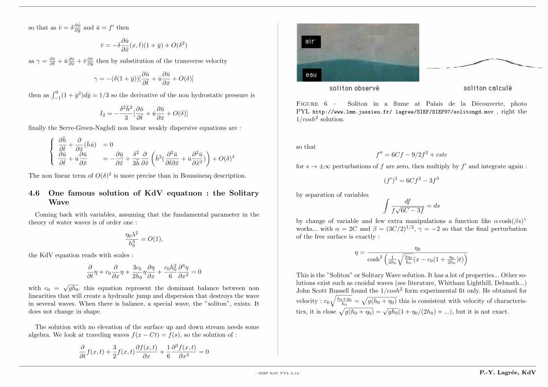
Figure 6 – Soliton in a flume at Palais de la Decouverte, photoPYL http://www.lmm.jussieu.fr/ lagree/SIEF/SIEF97/solitongd.mov , right the1/cosh2 solution.

so thatf ′′ = 6Cf − 9/2f2 + cste

for s→ ±∞ perturbations of f are zero, then multiply by f ′ and integrate again :

(f ′)2 = 6Cf2 − 3f3

by separation of variables ∫df

f√

6C − 3f= ds

by change of variable and few extra manipulations a function like α cosh(βs)γ

works... with α = 2C and β = (3C/2)1/2, γ = −2 so that the final perturbationof the free surface is exactly :

η =η0

cosh2(

12h0

√3η0h0

(x− c0(1 + η02h0

)t))

This is the ”Soliton” or Solitary Wave solution. It has a lot of properties... Other so-lutions exist such as cnoidal waves (see literature, Whitham Lighthill, Debnath...)John Scott Russell found the 1/cosh2 form experimental fit only. He obtained for

velocity : c0

√h0+η0h0

=√g(h0 + η0) this is consistent with velocity of characteris-

tics, it is close√g(h0 + η0) =

√gh0(1 + η0/(2h0) + ...), but it is not exact.

- MHP KdV PYL 2.14- P.-Y. Lagree, KdV

Figure 7 – 3 solitons of various selfsimilar shape ε0/ cosh2(

12

√3ε0x

), they are

in the moving frame. The larger the height, the thinner the width, the faster thewave. Time increases from bottom to top.

- MHP KdV PYL 2.15- P.-Y. Lagree, KdV

4.7 What about viscosity ?

Of course the viscosity plays a role and destroys the solitary wave. Let us lookat the influence of the up to now neglected viscous term.

At dominant order, we have computed the ideal fluid solution, for the boundary

layer, we must add the dominant viscous term 1Re

∂2u0

∂y2 in the momentum equation

∂u0

∂t= −∂η0

∂x+

1

Re

∂2u0

∂y2

with y = −1 + 1<1/2 y, and u0 = u0 we change the scales to be in the boundary

layer as usual. We refer to the moving frame ∂∂x = ∂

∂ξ , and ∂∂t = − ∂

∂ξ . we obtain

∂

∂ξu0 +

∂2u0

∂y2=

∂

∂ξη0

with boundary conditions, first the no slip u0 = 0 in y = 0, second the matching

u0(y →∞) = u0(y → −1) = η0(−1).

the resolution has been proposed by Kakutani & Matsuuchi in 1971 ([8]. Theproblem is to solve for f = u0 − η0(ξ,−1)

∂

∂ξf +

∂2

∂y2f = 0

with boundary conditions, first f = −η0 in y = 0, second f(y →∞) = 0 in fourier

space ikf + f ′′ = 0, so the solution is in e−σy with σ = (1−i)√2

(k sgn(k))1/2, then

u0 = η0 −∫η0e−σeikξdk

from this expression, we compute the transverse velocity using the trick of thevelocity in the boundary layer (second order effect, the blowing of the displacementthickness in the ideal fluid) see http://www.lmm.jussieu.fr/~lagree/COURS/

CISM/blasius_CISM.pdf

v1 = −∂u0

∂ξy +

1

Re1/2

∫ ∞−1

(∂

∂ξ(u0 − u0))dy

the corrective term, due to the blowing is rewritten after integration

vBL =1

(2Re)1/2

∫ ∞−∞

(−1 + isgn(k)|k|1/2η0eikξdk

by convolution, we K& M wrote

vBL =1

(πRe)1/2

∫ ∞ξ

∂η0

∂ξ′dξ′

(ξ′ − ξ)1/2

this velocity is inserted in the 1δ2∂φ∂y = ∂η

∂t + ε∂φ∂x∂η∂x

−f ′′(x, t)(1 + εη) + δ2f ′′′′(x, t)−1

3− vBL =

∂η

∂t+ ε

∂φ

∂x

∂η

∂x.

The final Kakutani & Matsuuchi [8] is

∂

∂τη0 +

3

2η0∂η0

∂ξ+

1

6

∂3η0

∂ξ3=

1

(πRe)1/2

∫ ∞ξ

∂η0

∂ξ′dξ′

(ξ′ − ξ)1/2

In the integral one recognises a ”fractional” derivative. As the Fourier transformof f is f , the the Fourier transform of d

nfdxn is (−ik)nf . Here, in this problem we have

(−ik)1/2, so a 1/2 derivative ! by inverse transform and convolution this (−ik)1/2

gives the part∫∞ξ

dξ′

(ξ′−ξ)1/2The final

∂

∂τη0 +

3

2η0∂η0

∂ξ+

1

6

∂3η0

∂ξ3+

1

(πRe)1/2

∂1/2η0

∂ξ1/2= 0

note that the coefficients are maybe wrong (check, it depends on the definitionof the 1/2 derivative). See le Meur https://hal.archives-ouvertes.fr/

hal-00826564/document for discussion and bibliography, and controversy of theuse of Fourier transform, Laplace transform must be better to take into accountthe history of the development of the boundary layer.

We note that the KM equation is not only local : with ∂ξ and ∂τ derivatives.This equation is as well non-local :

∫dξ′. The mix of properties makes it difficult

to solve and interesting to study.

- MHP KdV PYL 2.16- P.-Y. Lagree, KdV

4.8 The ondular bore or Mascaret

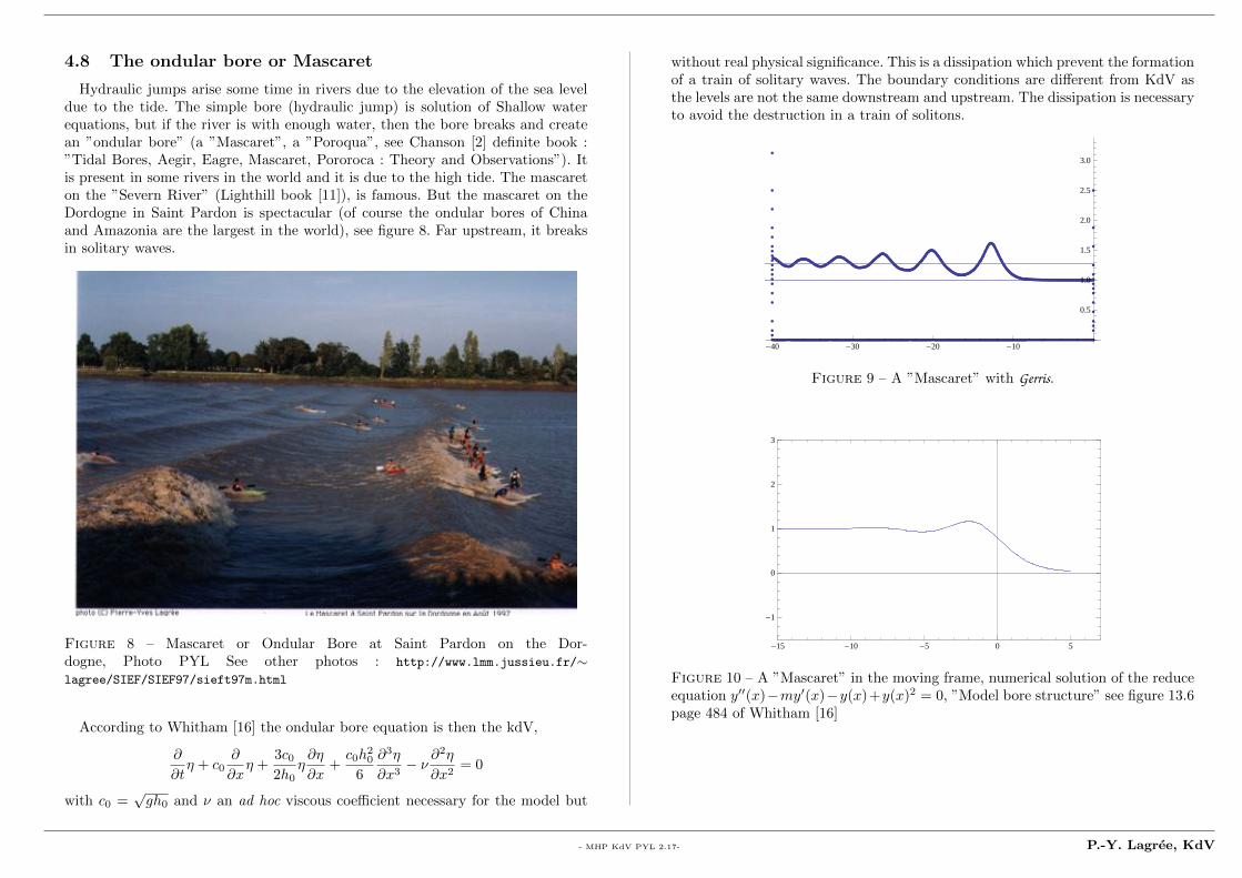
Hydraulic jumps arise some time in rivers due to the elevation of the sea leveldue to the tide. The simple bore (hydraulic jump) is solution of Shallow waterequations, but if the river is with enough water, then the bore breaks and createan ”ondular bore” (a ”Mascaret”, a ”Poroqua”, see Chanson [2] definite book :”Tidal Bores, Aegir, Eagre, Mascaret, Pororoca : Theory and Observations”). Itis present in some rivers in the world and it is due to the high tide. The mascareton the ”Severn River” (Lighthill book [11]), is famous. But the mascaret on theDordogne in Saint Pardon is spectacular (of course the ondular bores of Chinaand Amazonia are the largest in the world), see figure 8. Far upstream, it breaksin solitary waves.

Figure 8 – Mascaret or Ondular Bore at Saint Pardon on the Dor-dogne, Photo PYL See other photos : http://www.lmm.jussieu.fr/∼lagree/SIEF/SIEF97/sieft97m.html

According to Whitham [16] the ondular bore equation is then the kdV,

∂

∂tη + c0

∂

∂xη +

3c02h0

η∂η

∂x+c0h

20

6

∂3η

∂x3− ν ∂

2η

∂x2= 0

with c0 =√gh0 and ν an ad hoc viscous coefficient necessary for the model but

without real physical significance. This is a dissipation which prevent the formationof a train of solitary waves. The boundary conditions are different from KdV asthe levels are not the same downstream and upstream. The dissipation is necessaryto avoid the destruction in a train of solitons.

-40 -30 -20 -10

0.5

1.0

1.5

2.0

2.5

3.0

Figure 9 – A ”Mascaret” with Gerris.

-15 -10 -5 0 5

-1

0

1

2

3

Figure 10 – A ”Mascaret” in the moving frame, numerical solution of the reduceequation y′′(x)−my′(x)−y(x)+y(x)2 = 0, ”Model bore structure” see figure 13.6page 484 of Whitham [16]

- MHP KdV PYL 2.17- P.-Y. Lagree, KdV

Figure 11 – ondular bore in a channel ENSTA experimen-tal lab. Batterie de l’Yvette, photo PYL. See other films :http://www.lmm.jussieu.fr/∼lagree/SIEF/SIEF97/MAQUETTE/mascaret.html

Figure 12 – A hydraulic jump is metamorphosed in a undular bore due to a smallincrease in depth. photo PYL, Baie de la Fresnaye (22) Port a la Duc. [click tolaunch the movie, Adobe Reader required]

Figure 13 – Some meters down stream, the hydraulic jump changes ... into anundular bore photo PYL, Baie de la Fresnaye (22) Port a la Duc.

- MHP KdV PYL 2.18- P.-Y. Lagree, KdV

Figure 14 – left a very non linear wave Miami 2016, right a mascaret SaintPardon 1997...

5 Conclusion

In this chapter, we observed waves in water. First, we study waves of smallamplitude ε � 1 in shallow water δ � 1. This gives the ∂’Alembert waveequation. Second, we study waves of small amplitude ε � 1 in deep water δ = 1.This is Airy wave theory. Third, we study waves in not small amplitude ε = 1in shallow water δ � 1. This is shallow water. Finally we study waves of smallamplitude ε� 1 in shallow water δ � 1 but no so shallow, with ε = δ2 � 1. Thisis Boussinesq KdV theory.

The Soliton and the Ondular Bore are nice examples of waves.

References

[1] Magnar Bjørkavag, Henrik Kalisch Wave breaking in Boussinesq models forundular bores Physics Letters A 375 (2011) 1570–1578

[2] H. Chanson (2011), ”Tidal Bores, Aegir, Eagre, Mascaret, Pororoca : Theoryand Observations”, Word Scientific googlebook

[3] F. Coulouvrat, notes de Cours de DEA de Mecanique LMM/UPMC, Intro-duction aux Methodes Asymptotiques en Mecanique.

[4] Debnath L. (1994) ”Nonlinear Water Waves” Academic Press.

[5] Lokenath Debnath Nonlinear Partial Differential Equations for Scientists andEngineers googlebook

[6] J.E. Hinch Perturbation Methods, Cambridge University Press, (1991)

[7] J. Kevorkian & J.D. Cole, Perturbation Methods in Applied Mathematics,Springer (1981)

[8] T. Kakutani & K. Matsuuchi, ”Effect of viscosity of long gravitywaves”(1975), J. Phys. Soc. Japan 39 No 1 pp. 237-246.

[9] H. Lamb, hydrodynamics

[10] Landau Lifshitz

[11] Lighthill J. (1978) ”Waves in fluids” Cambridge Univ. press

[12] Newell A. C. (1985) : ”Solitons in mathematics and physics”, SIAM RCSAMno48

[13] Peyrard Dauxois Physique des solitons

[14] Gerard A. Maugin Solitons in elastic solids (1938–2010) Mechanics ResearchCommunications 38 (2011) 341–349

[15] Michel Remoissenet (1999) Waves Called Solitons : Concepts and Experimentsgooglebook

[16] Gerald Beresford Whitham, ”Linear and Nonlinear Waves” Wiley-Interscience1974 googlebook

http://en.wikipedia.org/wiki/Korteweg-de_Vries_equation

http://en.wikipedia.org/wiki/Airy_wave_theory

up to date 15 novembre 2021

This course is a part of a larger set of files devoted on perturbations methods,asymptotic methods (Matched Asymptotic Expansions, Multiple Scales) andboundary layers (triple deck) by P.-Y . L agree .The web page of these files is http://www.lmm.jussieu.fr/∼lagree/COURS/M2MHP.

/Users/pyl/ ... /kdv.pdf

- MHP KdV PYL 2.19- P.-Y. Lagree, KdV

Figure 15 – From the book Sir James Lighthill and Modern Fluid MechanicsLokenath Debnath

- MHP KdV PYL 2.20- P.-Y. Lagree, KdV

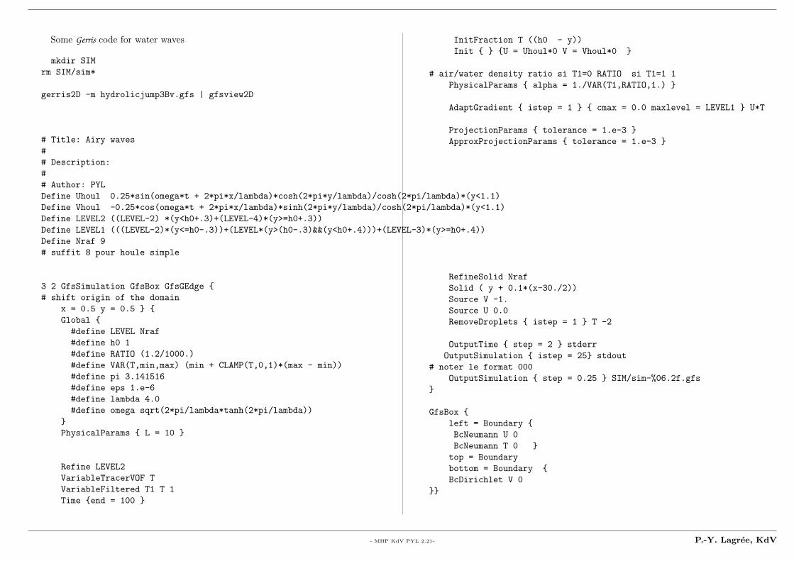
Some Gerris code for water waves

mkdir SIM

rm SIM/sim*

gerris2D -m hydrolicjump3Bv.gfs | gfsview2D

# Title: Airy waves

#

# Description:

#

# Author: PYL

Define Uhoul 0.25*sin(omega*t + 2*pi*x/lambda)*cosh(2*pi*y/lambda)/cosh(2*pi/lambda)*(y<1.1)

Define Vhoul -0.25*cos(omega*t + 2*pi*x/lambda)*sinh(2*pi*y/lambda)/cosh(2*pi/lambda)*(y<1.1)

Define LEVEL2 ((LEVEL-2) *(y<h0+.3)+(LEVEL-4)*(y>=h0+.3))

Define LEVEL1 (((LEVEL-2)*(y<=h0-.3))+(LEVEL*(y>(h0-.3)&&(y<h0+.4)))+(LEVEL-3)*(y>=h0+.4))

Define Nraf 9

# suffit 8 pour houle simple

3 2 GfsSimulation GfsBox GfsGEdge {

# shift origin of the domain

x = 0.5 y = 0.5 } {

Global {

#define LEVEL Nraf

#define h0 1

#define RATIO (1.2/1000.)

#define VAR(T,min,max) (min + CLAMP(T,0,1)*(max - min))

#define pi 3.141516

#define eps 1.e-6

#define lambda 4.0

#define omega sqrt(2*pi/lambda*tanh(2*pi/lambda))

}

PhysicalParams { L = 10 }

Refine LEVEL2

VariableTracerVOF T

VariableFiltered T1 T 1

Time {end = 100 }

InitFraction T ((h0 - y))

Init { } {U = Uhoul*0 V = Vhoul*0 }

# air/water density ratio si T1=0 RATIO si T1=1 1

PhysicalParams { alpha = 1./VAR(T1,RATIO,1.) }

AdaptGradient { istep = 1 } { cmax = 0.0 maxlevel = LEVEL1 } U*T

ProjectionParams { tolerance = 1.e-3 }

ApproxProjectionParams { tolerance = 1.e-3 }

RefineSolid Nraf

Solid ( y + 0.1*(x-30./2))

Source V -1.

Source U 0.0

RemoveDroplets { istep = 1 } T -2

OutputTime { step = 2 } stderr

OutputSimulation { istep = 25} stdout

# noter le format 000

OutputSimulation { step = 0.25 } SIM/sim-%06.2f.gfs

}

GfsBox {

left = Boundary {

BcNeumann U 0

BcNeumann T 0 }

top = Boundary

bottom = Boundary {

BcDirichlet V 0

}}

- MHP KdV PYL 2.21- P.-Y. Lagree, KdV

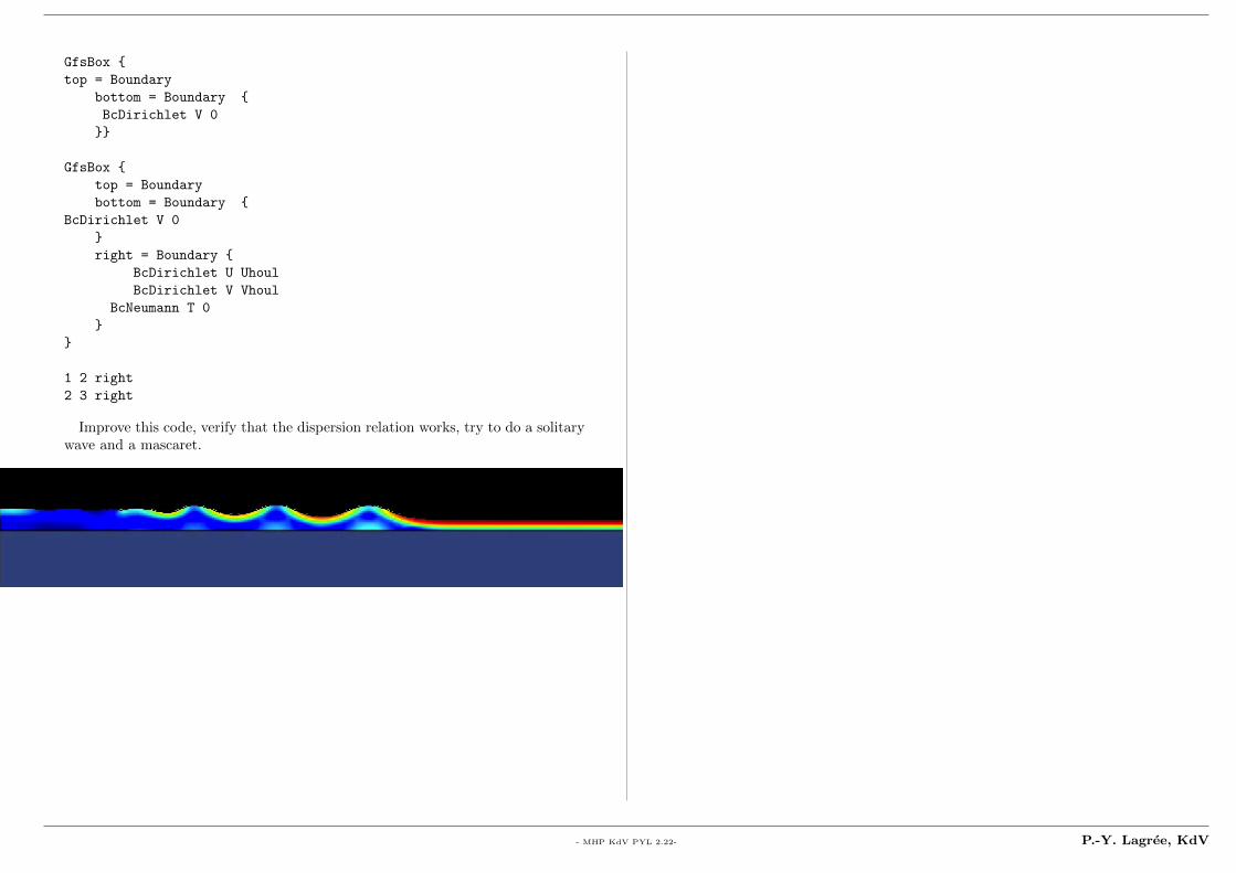
GfsBox {

top = Boundary

bottom = Boundary {

BcDirichlet V 0

}}

GfsBox {

top = Boundary

bottom = Boundary {

BcDirichlet V 0

}

right = Boundary {

BcDirichlet U Uhoul

BcDirichlet V Vhoul

BcNeumann T 0

}

}

1 2 right

2 3 right

Improve this code, verify that the dispersion relation works, try to do a solitarywave and a mascaret.

- MHP KdV PYL 2.22- P.-Y. Lagree, KdV

Here code for Saint Venant hydraulic jump (the bore)

# Title: Steady Hydraulic Jump

#

# Description:

#

# Author: PYL

# Command: gerris2D dam.gfs

# Required files: dam.plot

# Generated files: jump.gif

##

# F1^2 0.375

# F2^2 0.

# h1 1

# h2 0.5

# W 1.22474

#

#Define L0 10

#

# Use the GfsRiver Saint-Venant solver

1 0 GfsRiver GfsBox GfsGEdge {} {

PhysicalParams { L = 10 }

RefineSolid 9

# Set a solid boundary close to the top boundary to limit the

# domain width to one cell (i.e. a 1D domain)

Solid (y/10. + 1./pow(2,9) - 1e-5 - 0.5)

# Set the topography Zb and the initial water surface elevation P

Init {} {

Zb = 0

U = 0.387632*(x<-3)+(-.22474*0.5)*(x>-3)

P = {

double p = x < -3 ? 1 : 0.5;

// p = 1+(1.30277563773199-1)*(1+tanh(x))/2;

return MAX (0., p - Zb);

}

}

PhysicalParams { g = 1. }

# Use a first-order scheme rather than the default second-order

# minmod limiter. This is just to add some numerical damping.

AdvectionParams {

# gradient = gfs_center_minmod_gradient

gradient = none

}

Time { end = 7}

OutputProgress { istep = 10 } stderr

# Save a text-formatted simulation

OutputSimulation { step = 0.1 } sim-%g.txt { format = text }

# Use gnuplot to create gif images

EventScript { step = 0.1 } {

time=‘echo $GfsTime | awk ’{printf("%4.1f\n", $1);}’‘

cp sim-$GfsTime.txt sim.txt

cat <<EOF | gnuplot

load ’dam.plot’

set title "t = $time"

set term postscript eps color 14

set output "sim.eps"

h(x)= 1-(0.5)*(x>-3+1.*$time)

plot [-5.:5.][0:2]’sim-$GfsTime.txt’ u 1:7:8 w filledcu lc 3, ’sim-0.txt’ u 1:7 w l lw 4 lc 1 lt 1,h(x)

EOF

time=‘echo $GfsTime | awk ’{printf("%04.1f\n", $1);}’‘

convert -density 300 sim.eps -trim +repage -bordercolor white -border 10 -resize 640x282! sim-$time.gif

rm -f sim.eps

}

# 1:x 2:y 3:z 4:P 5:U 6:V 7:Zb 8:H 9:Px 10:Py 11:Ux 12:Uy 13:Vx 14:Vy 15:Zbx 16:Zby

# Combine all the gif images into a gif animation using gifsicle

EventScript { start = end } {

gifsicle --colors 256 --optimize --delay 25 --loopcount=0 sim-*.gif > mjump.gif

rm -f sim-*.gif sim-*.txt

}

}

GfsBox {

left = Boundary { BcNeumann U 0 }

right = Boundary { BcNeumann U 0 }

}

- MHP KdV PYL 2.23- P.-Y. Lagree, KdV

rivière

montée de marée

ressaut

Ressaut mobile

U1 = 0.3876 U2 = -0.22474 h1 = 1 h2= 0.5 W=1

h1 h2

Figure 16 – bore at Port a la Duc, baie de la Fresnaye. Photo PYL and withGerris

. .

Raymond Subes ”Sans Titre” 1961 (entree de Jussieu Quai Saint Bernard)

- MHP KdV PYL 2.24- P.-Y. Lagree, KdV