SLAC-PUB-2140 June 1978

INTRODGTION TO INTENSITY INTERFEROMETRY FOR NUCLEAR-PARTICLE PHYSICISTS'

Alan Katz Stanford Linear Accelerator Center

Stanford University, Stanford, California 94305

ABSTRACT

The Hanbury-Brown and Twiss method for measuring the radii of stars

also has interesting applications in other realms of physics. Intensity

interferometry, the technique used by Hanbury-Brown and Twiss for their

star measurements, should yield analogous information about the angular . -

sizes of excited particles and nuclei, which emit secondary particles. In

this report, we interpret such emissions and the correlation functions

that arise from considering registration probabilities at two space or time

points in terms of the language of optics and diffraction theory. Our

objective is to review the physics involved in the Hanbury-Brown and Twiss

effect and to point out possible applications to problems in nuclear and

particle physics.

(Submitted for Publication)

Work supported by the Department of Energy.

-2-

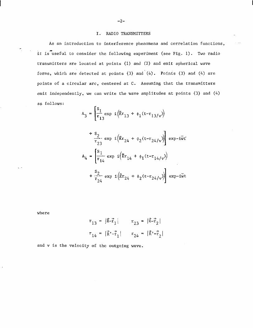
1. RADIO TRANSMITTERS

As an introduction to interference phenomena and correlation functions, ~-

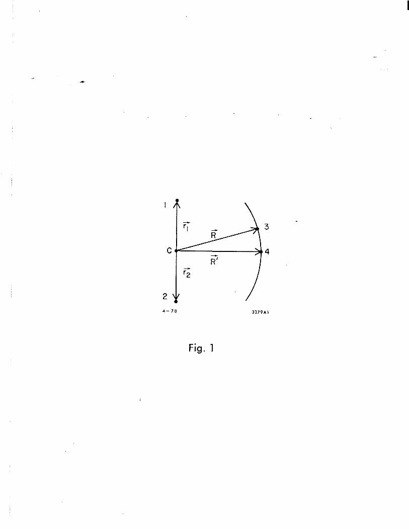
it is%seful to consider the following experiment (see Fig. 1). Two radio

transmitters are located at points (1) and (2) and emit spherical wave

forms, which are- detected at points (3) and-(4). Points (3) and (4) are

points of a circular arc, centered at C. Assuming that the transmitters

emit independently, we can write the wave amplitudes at points (3) and (4)

as follows:

A = 3 exp i&l3 ( + "l(t-r13,v))

&24 + f$2(t-r24,v exp-i&

A4 = + Vt-r14/v

+ s2 exp i(k24 '24

+ '2(t-r24/v exp-Gt

where

r13 = Ii&T1 1 '23 = I&s,1

r14 = litG,i r24 = lii1-Z21

and v is the velocity of the outgoing wave.

-3-

Remarks

1. We have assumed that both detectors emit wave packets strongly

peake;about the wave number, K.

2. The functions $1 and c$, are, in general, time dependent (real)

functions which set the phases of the transmitters.

3. For convenience, we will assume Sl =S and that these amplitudes 2

are time independent.

In most situations of interest, IQ ” lq,lq’ Using this inequality, we can write:

I$-gil = [(g-?i)*(ft-:i)]h = (R2 + r: - 2g.gi)&

Second-order terms in have been ignored.

Similarly, lit'-;;1 z (R-fi'*:i) .

Hence, we can estimate A3 and A4 as follows:

-4-

In classical electromagnetic theory, we might think of A 3 and A4 as components

of the electric or magnetic field. The intensity of the electromagnetic

disturbance at points (3) and (4), then, is respectively:

+ exp -i[~(ff.(~2-:1)+(02-~~)l]

2ls1 I2 = R2

II

For fixed phase functions ($1 and c$~ independent of time), the conditions

on the argument of the cosine functions that define the intensity maxima

and minima are easily found. However, if 41 and $I, are random functions

of time (such that the phase jumps around a lot in the time interval necessary

to make the measurement), then it is necessary to average I3 and I4 over

a time interval long compared to the interval between an average jump. In

this case, I3 and I4 reduce to (constant) x 21S112/R2, and it is seen that

all spatial dependence is lost.

However, a harmonic spatial dependence results when the product of

I3 and I4 is taken prior to performing the average, provided that points

(3) and (4) are within a "coherence" length of each other:

-5-

1314 c IAJ2/~J2 = 4'~$+(1 + co.+] + cosb] + cos [a]cosb]) ~-

where 4

Making use of the trigonometric identity

we find:

cos a cos b ,= k cos(a-b) + % cos(a+b) ,

+ cos k]+l+% cos([a]-[b])3, ' cos( b]+[b] )]

+ cos b] + cos @I+% cos R-6’ -?2

V

33 cos(-[a]+@] ) 1 . Now, if the detectors are sufficiently close such that (R'-i).s, and

(&ii> ';tl are small compared to the coherence length (the distance over

which interference phenomena are appreciable or, for this example, (v X

the average time between phase jumps Z Rcoherent)), then

Thus 41s114

<I,I,>’ = R4 [1+$ cosIK(l[i-lP)'(~2-:1)~

-6-

It may be concluded that even if the average intensity shows no variation over

the circle, the product of the intensities at two points sufficiently near

each c&her will still display a harmonic variation (in spatial coordinates).

For this reason,<1314> is called a correlation function. An explanation

for such a correlation is not hard to come by; it is a reflection of the

fact that any phase change that affects the wave amplitude at a given point

on the circle will simultaneously affect the amplitudes at all points

within a coherence length of the given point. This implies that the degree

of correlation between points (3) and (4) is preserved: For example, if

a maximum at (3) implies a maximum at (4), then a minimum at (3) implies

a minimum at (4).

The circular arrangement of detectors that we have been discussing is

special in the sense that for ~~2~,~~1~ << kCOHERENCE <IRIS> is spatially

dependent for every pair of points on the circle. For our example, then,

. - we need not be too concerned with coherence length and times as long as the

above condition on j:2/ and jZ,l is met.

II. TIME CORRELATIONS

Time correlations are a natural extension of what has been done so

far. The precise meaning of a time correlation (as opposed to the spatial

correlation considered above) is made evident by examining once more our

experiment with two radio transmitters. Now, however, the transmitters

will be emitting at different frequencies, w 1 and w 2' Moreover, the two

detectors will be placed at the same spatial point. The correlation

function that will be of interest is of the form 13(t)13(t +r ), where

13(t) is the intensity reading at point (3), at time t, and 13(t+'r) is

the intensity reading at the same point but at the delayed time, t+r.

A3(t) = R exp "' [ (t - 'i3)-ilt)+ exp i(K2r23+$2 (t - +)G2t)] -

A3 (t+r) = :[exp i(Rlr13+ml(t+r - %)-cl(t+l))

+ exp i(E2r23+$2 (t+= - F)-i2(tfT )]

The intensities at the two time points are proportional to:

ISl12 IA,(t)12 = '7 (t - %)-o, (t - %)+G2-;1) t)

( - g-o2 (t - t

-iir +$ 2 23 1 (t - F)-$2 (t - ~)+(G2-q t

and

2/q2 - IA3W-d I2 = R2 [ l+cos Klr13-!?2r23+$1 /

-9, +(W,-W,) (t+T)

Hence, the time average of the product of intensities is given, to within

a proportionality factor, by:

-8-

Now, for T < tC (the coherence time), we have:

41s114

Hence, there is a harmonic variation in T only if r < tC and w2 # G1.

Applications of the concept of time correlation and further disGussion of

coherence time, as related to the spectral width, can be found in Born

and Wolf, Principles of Optics, 5th Ed., § 10.7.3.

III. CONTINUOUS, ALMOST MONOCHROMATIC SOURCE

We now take up the more complicated problem of determining the correl-

ation function for two points on a screen illuminated by a continuous

monochromatic source. ' This problem serves both to expand the notion of

the correlation function and to provide a connection between the correlation

function and diffraction theory (via the Van Cittert-Zernike Theorem).

This connection will prove useful when we discuss the emission of particles

from an excited nucleus.

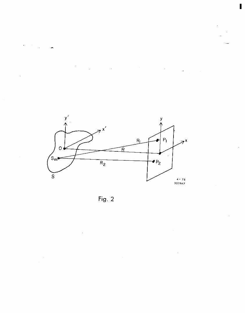
The extended source (x',y')--see Fig. 2--is taken to be parallel to

the plane, (x,y). Moreover, the overall dimensions of the source are

assumed to be small compared to the distance R. For the purpose of cal-

culating the total disturbance at a point, P, it is useful to divide (x',y')

into sections small compared to the wavelength of the disturbance and,

then, to sum the

countable number

p1 and P2 are

11

contributions from each of these sections. For a

of sections, the total disturbances registered at points

y ,(t> = c VlmW , v2(t) =-xv m 2m

(t> m

respectively.

-9-

Making use of the fact that

<( v1 REAL1 (t) VdRML) (t)) -

is proportional to <Vl(t)Vt(t)>, and that Vi(t) and V,(t) are complex, 2

we define the following correlation function:

W1,P2) = <vl(tN;w> = (yJml~“~$2w>

= c (Vml wv~2w> m,n

= z<vrnl w;2(t)) m

+ c c <Vmlw~2w> mn

Now, for m # n, we can write m#n

<vml (t)vz2(t)) = <vml(t,)(V~2(t)\) = 0

The first equality follows from the statistical independence of the sources

whereas the second equality can be confirmed by allowing-the functions

Vml(t) or Vn2(t) to have the functional form:

a Vml(t> = + exp i(mmlk- +))exp i(iir-Gt)

(This form of Vml(t) is derived under the assumption that the wave packet

is very strongly peaked about the wavenumber E). Hence,

<Vml(t)$2(t)) = F? <exp iQml(t))<exp-iBm2(t)) ml n2

= 0 .

-lO-

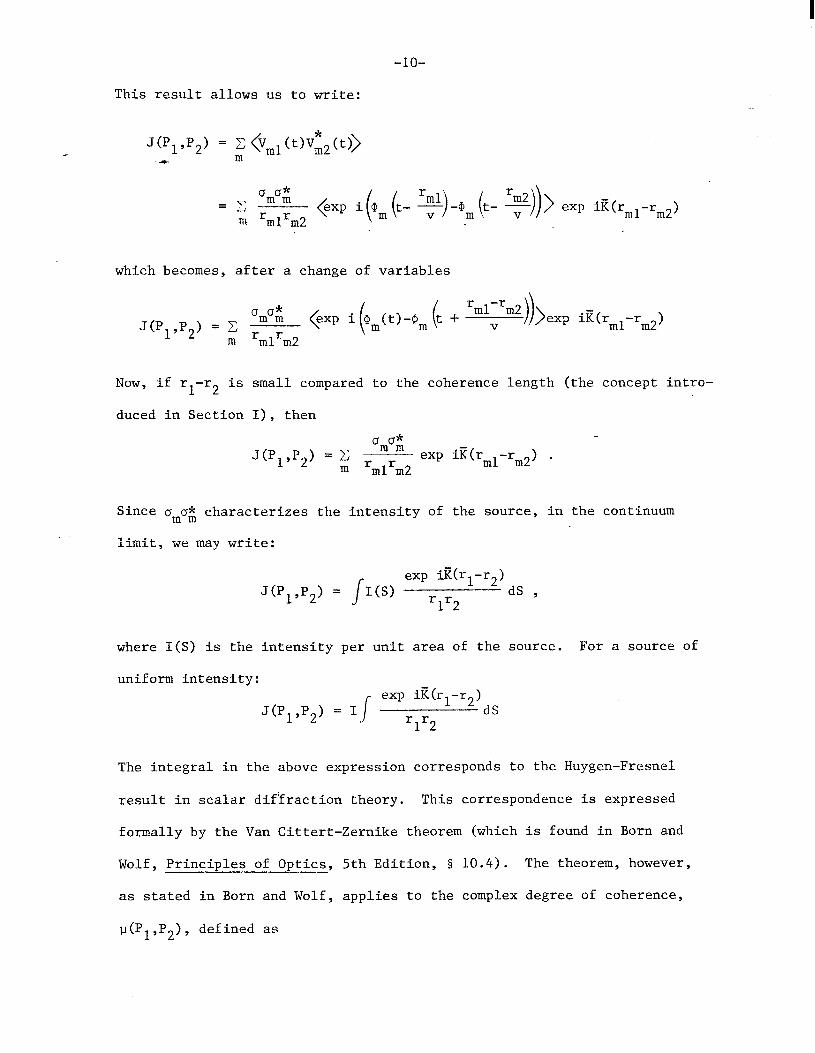
This result allows us to write:

J (5 ,P2) = C em1 (t)$, (t>> 4 m

=C m lcrn2 (exp i(m,(t- %)-Qm(t- +))> exp iK(rml-rm2)

which becomes, after a change of variables

orno: 'mlwrm2 JP1,P2) = C v exp ii?(rml-rm2)

m rmlrm2

Now, if rl-r2 is small compared to the coherence length (the concept intro-

duced in Section I), then

J(P1,P2) = C m

m m exp iE(rml-rm2) . rmlrm2

Since orno& characterizes the intensity of the source, in the continuum

limit, we may write:

J(P1,p2) = JI(S) exp it(r,-r,)

rlr2 dS ,

where I(S) is the intensity per unit area of the source. For a source of

uniform intensity:

J(P1,P2) = Ij exp iK(rl-r2)dS

rlr2

The integral in the above expression corresponds to the Huygen-Fresnel

result in scalar diffraction theory. This correspondence is expressed

formally by the Van Cittert-Zernike theorem (which is found in Born and

Wolf, Principles of Optics, 5th Edition, § 10.4). The theorem, however,

as stated in Born and Wolf, applies to the complex degree of coherence,

u(P1,P2), defined as

-ll-

U(P1,P2) = J (P1 3,)

J(P1,P1)J(P2,P2) 2

Born and Wolf go on to show that

lJ(pl,P2) = (exp iY)/fi(x',y')exp-iE(px'+qy')dx'dy'

/I" I(x',y')dx'dy'

where (x',y') are the coordinates of a typical source point, S; (X1,Y1)

and (X Y ) 2' 2 are the coordinates of P1 and P2; and p, q, and Y are defined

as follows:

(x1-x2> R 'P

(V2) = R 4

Y = &[( x;+y;, - (x$+Yy

For the particular example of a uniform circular source of radius, a,

Born and Wolf3 compute:

exp iY

where

f ((xl-x2)2+(Yl-Y2)2)L . v=-

IV. APPLICATION TO NUCLEI

The approach of Hanbury-Brown and Twiss to the measurement of stellar

radii (which involves the computation of a correlation function related

to 6314)) is applicable to the emission of particles from an excited

nucleus4; in place of a star, we deal with an excited nucleus that emits

neutrons or pions. It is necessary, however, to distinguish the pion

problem from the neutron one in terms of the statistics the particles

-12-

obey. Pions are spin 0 particles and must be described by overall

symmetric wave functions whereas neutrons are spin $ and have antisymmetric

wave Qnctions. The consequences of this distinction will be discussed

below.

As a first attempt at understanding the nuclear problem, we will

consider the nucleus to have been excited since the beginning of time

(t=O) and to be kept excited by a continual input of energy. In a proper

treatment, the nucleus is excited at a particular time and decays exponentially.

Suppose now that we examine the particle emissions from the point of

view of Section I. Two points on the nuclear surface may be regarded as

independent emittersg that is, if we consider a large ensemble of similarly

excited nuclei, then any two points on the nuclear surface will be completely

uncorrelated after averaging over the ensemble. Next, we set up two

detectors and ask what the probability is for registering one particle in

. - each detector at a time, t. The two surface elements lie sufficiently close

to each other that it is impossible to decide from which source a particular

particle came: The wave functions of the two emitted particles overlap.

The means by which this ambiguity is incorporated into the formal description

of the system is to treat the outgoing particles as identical bosons or

fermions and, accordingly, to symmetrize or antisymmetrize the wave function.

When pions are simultaneously detected, the wave function is given by

(see Fig. 3):

A zi exp i(p3r13-E3t) /A exp i(p4r24- E t)/A 4

R '13 '24

+ ew i(P4r14 -E t)//I exp i(p3r23-E3t)& 4

'14 '23

-13-

It should be noted that the detectors record the energies of the particles.

There is no need to worry about the spin part of the wave function 4

since pions are spinless particles. Under particle exchange, which is

effected most easily by switching the "1" and “2” indices, the amplitude

A= is seen to be symmetric.

The probability for detecting two pions simultaneously is given by:

1 AT 1 2 = &- b+cos (p3(r13-r23)+P4 (r24-r14$]

with

Next, we assume that the particles received by the detectors are spin

k nucleons. In this case, there is a spin component of the wave function

as well as a spatial part to consider. Assuming that the polarization of . -

the nucleons is not fixed, we must give equal weight to the six possible

antisymmetric wave functions for a two-state system:

(1 .) G = i(la>lb>-lb>la>) 1 -t--f>

a>

space spin

b>-lb>la>)

(5) G = la>la> L(lfG>-IC+>) LT

(6) $ = /b>lb,;(/W-I++>)

-14-

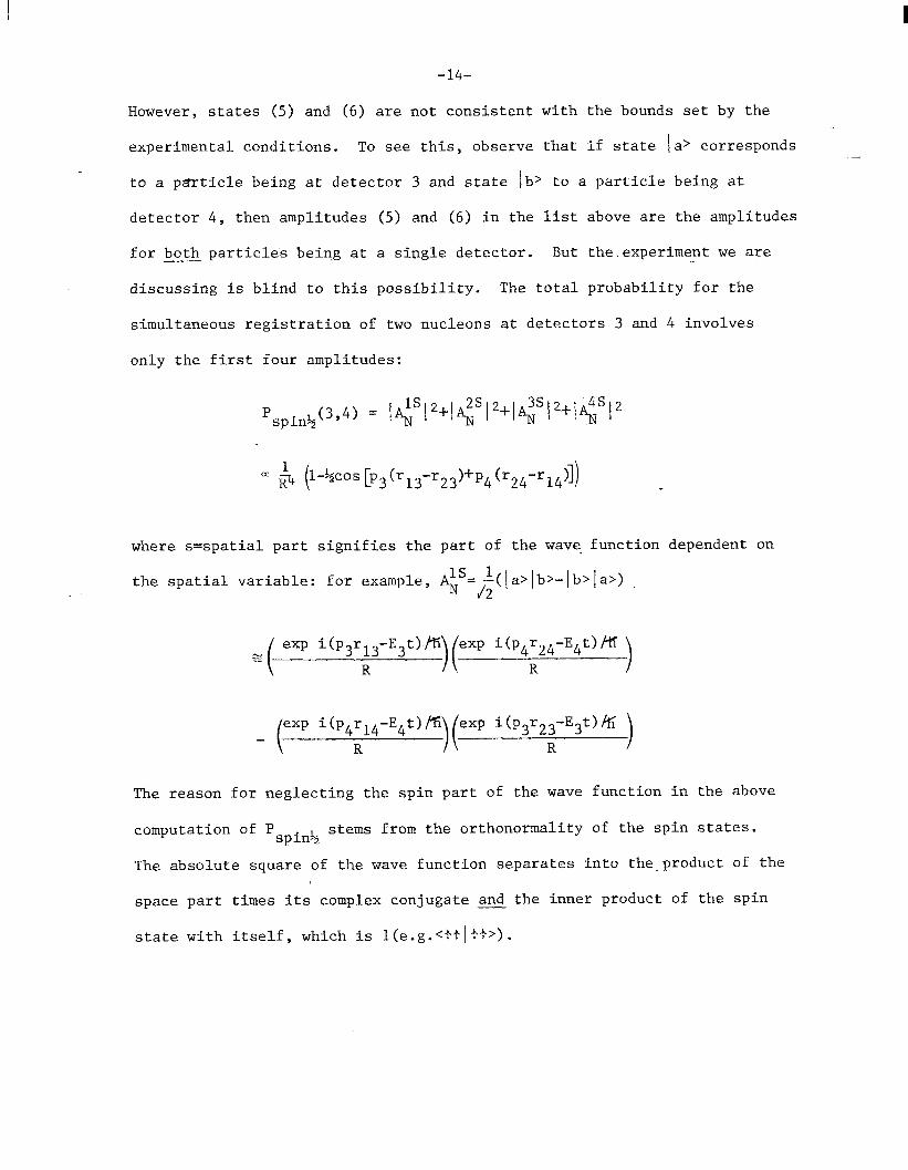
However, states (5) and (6) are not consistent with the bounds set by the

experimental conditions. To see this, observe that if state a> corresponds

to a p8rticle being at detector 3 and state lb> to a particle being at

detector 4, then amplitudes (5) and (6) in the list above are the amplitudes

for both partic1e.s bein,g at a single detector. But the.experiment we are

discussing is blind to this possibility. The total probability for the

simultaneous registration of two nucleons at detectors 3 and 4 involves

. -

only the first four amplitudes:

P spin%C3P4) = 14”

where s=spatial part signifies the part of the wave function dependent on

the spatial variable: for example, <"= I(la>lb>-lb>la>)- J2

sz exp i(p3r13-E3t)fi exp i(p4r24-E4t)kK

R R

exp i(p4r14-E4t)fi -( exp i(p3r23-E3t)/r;

R R

The reason for neglecting the spin part of the wave function in the above

computation of P spin+ stems from the orthonormality of the spin states.

The absolute square of the wave function separates into the-product of the

space part times its complex conjugate and the inner product of the spin

state with itself, which is l(e.g.<f+lf+>).

-15-

V. APPLICATION TO NUCLEI: CONTINUOUS SOURCE

S: far, we have dealt only with a source composed of two independent

emitters. The next step is to calculate the registration probability for

an extended source. A'useful example is the uniformly radiating sphere.

Before turning to this example, we would like to treat a continuous

source in some generality. The tools needed for such a treatment can be

found in Section III. If Vml and Vm2 represent the wave amplitudes at Pl

and P 2, respectively, for particles originating from the mth source element,

then the total registration probability, W(P,,P,), for a countable set of

emitters is proportional to:

Nucleons: (1)

‘NC’1 ,‘+ xz 3<bml ctjVn2 (tbVnl (t>Vm2 tt) I’> mn

+ (I vml wn2 w+vnl WVm2 (t) 12>

Pions: (2)

WIT (5 J+ = = <km1 wn2 (t)+Vnl (mm2 (t> I’> mn

Some remarks are in order at this point:

1. The registration probabilities given above are those that enter

into the calculation of exclusive (as opposed to inclusive) cross sections.

In order to get a better feel for the sort of information contained in

either WN(P1,P2) or W,(P1,P2), let us consider a specific example. Suppose

that the source is composed of three distinct surface elements, each of

which emits particles independently of the other two. At any time, the

number of particles that may be emitted is zero, one, two, or three.

Clearly, since it takes two particles to trigger the detectors in the

-16-

experiment we have in mind, zero and one particle emissions are not

detectable events. With three particle emissions, however, it is possible

to havg one particle at each detector (and a third particle somewhere

else). But the final state of the source after the emission of three

particles is different from the state after a two-particle emission.

In computing WN(Pl,P2) and W,(P1,P2), we consider only events arising

from two particle emissions. This is what is meant by an "exclusive"

cross section. On the other hand, the "inclusive" cross section for our

two detector experiment would include all processes that lead to a final

state with one particle at each detector, regardless of the final state of

the source.

2. The second remark concerns the reason behind summing the individual

probabilities rather than summing the amplitudes first and then taking the

absolute square of the total amplitude. The reason is that the emission

of particles by a particular pair of nuclear surface elements leads to a

final state distinguishable from the rest.

Let us calculate WN(P1,P2):

wN(p1,p2) a<cc ~31Vml(t>Vn2(t)-Vn mn

I2 1 wm2 (t)

+ Ivml(t>vn2(t>+vnl(t)Vm20 I’)>

The first term arises from those states involving one of the three symmetric

spin states, whereas the second term is the spatial part of an overall anti-

symmetric wave function with an antisymmetric spin part. Observe that particles

originating from the same source element can make a finite contribution

to WN(P1,P2) so long as the spins of the particles are different.

-17-

WN(P1,P2) can be evaluated further:

w,(p1’p2)cc3cc <1vm~vn2-vn~vm2 I”> mn

+ 2 $ <~vmlvn2+vnlvm2 ! 2>

= 32% ( <lvm1121 v,,12)<IvnJ21vm212~

+” <lv~~121V~~12>+(lVn1121vm212> mn (

4! r, lVml 1 2 7; [vn2 1% <gvmlv;2 y;1vn2> m n

. -

-4<zv*v xv v*> . m ml m2 n nl n2

Renaming dummy indices, we have:

wN(p1,p2)ar2 [ ~Ivrnl12 zjvn212-%( z ml m2 m n

v v* > (ynl$2)*>] or

3J(p1’p2)a2 kjv,, 1 2 c,jvn2 I’-+( i’lvmlv;, 1 2)] * m

The sums in the first expression on the R.H.S. of the proportionality are

independent of time; thus, the time-average brackets have been dropped.

This result resembles the expressions of Section III, where the function

of major interest was J(P1,P2) =C, (ml(t)VE2(t)) . As long as rml-rm2

is small compared to the coherence length, we need not fret that

< ;vrng2 ~Nnlv~2,*> fi c <vm1v;2> ~<07nlv;2)*> : m

-18-

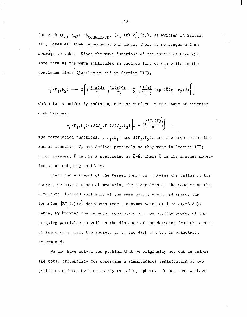
for with (rml-rm2) 'RCOHERENCE, (V,l (t> Vz2 (t> > 3 as written in Section

III, loses all time dependence, and hence, there is no longer a time

aver:ge to take. Since the wave functions of the particles have the

same form as the wave amplitudes in Section III, we can write in the

continuum limit (just' as we did in Section III),

wN(p1,p2) + 2[/-1($ds /'(:ids - +i,E exp iK(rl-r2)dS/2]

which for a uniformly radiating nuclear surface in the shape of circular

disk becomes:

wN(p1,~2)a2J(P1,P1)J(P2,P2) 1 [ _ gJ;q . ’

The correlation functions, J(P1,P1) and J(P2,P2), and the argument of the

Bessel function, V, are defined precisely as they were in Section III;

here, however, i? can be i nterpreted as F/&I, where 5 is the average momen-

tum of an outgoing particle.

Since the argument of the Bessel function contains the radius of the

source, we have a means of measuring the dimensions of the source: as the

detectors, located initially at the same point, are moved apart, the

function [2J1 (V)/V] d ecreases from a maximum value of 1 to O(V=3.83).

Hence, by knowing the detector separation and the average energy of the

outgoing particles as well as the distance of the detector from the center

of the source disk, the radius, a, of the disk can be, in principle,

determined.

We now have solved the problem that we originally set out to solve:

the total probability for observing a simultaneous registration of two

particles emitted by a uniformly radiating sphere. To see that we have

-19-

the solution at hand, it is necessary to show that the problem of a

uniformly radiating sphere reduces to the one of a uniformly radiating -

disk.- Consider an infinitesimal surface element on the radiating sphere.

The contribution of this element to the number of emitted particles in a

particular direction is proportional to the-projection'of the surface

onto a plane lying perpendicular to the direction line, D (which is defined

by the polar angles (u,@)--see Fig. 4). 6

The projection of a spherical

surface onto a plane normal to the direction (a,B) is just a circular

disk of radius equal to the radius of the sphere. Hence, the reduction

to a disk problem is accomplished.

VI. PROTON COLLISIONS

An interesting application of the ideas presented so far is the

mechanism for particle exchange between two colliding protons. The

. - particle that is exchanged can itself emit secondary particles. This

exchanged particle will be termed a gluon, although reggeon would be an

equally good term. If the pattern of emissions from the exchanged particle

is distinguishable from the emission pattern of the colliding protons,

then it might be possible to measure the size and shape of the "inter-

action" region by applying what was learned in the earlier sections.

Since opposing theories predict differently shaped reaction regions,

correlation measurements of secondary-particle emissions might be able to

point to the right theory.

As an illustration of future work that might be done, we will present

a multiperipheral picture of the proton-proton collision process (see

Figures 5 and 8a,b). Two well-collimated beams of protons, traveling in

opposite directions, are allowed to scatter off each other. When any two

-2o-

protons are sufficiently close, there is a possibility that they will

interact by exchanging a gluon. The gluon leaves one proton and dis-

'appeals at the other one. In-between, the exchanged gluon emits a few

secondary particles. To make the picture especially simple, we will

assume that the path, ,which the'exchanged gluon takes between the protons,

is straight and that the emission of a secondary particle at one point

along the path is completely uncorrelated with emissions at any other

point (We could equally well assume that the path taken by the gluon is

curved.). The important point is that after averaging over all curved

paths, the mean width of the path is small compared to its length. A

third assumption is that there is an equal probability for emission along

the path. Finally, the emission pattern of the secondary particles is

completely unaffected by any motion of the exchanged gluon. In some

sense, then, the exchanged gluon within this picture does not travel from

one proton to the other.

When an average over many collisions is taken, the emission problem

reduces to that of a uniformly radiating surface, almost rectangular in

shape but very narrow. 7 If two detectors are placed parallel to the radi-

ating slit (see Fig. 5), then the total probability for particles to

arrive simultaneously at the detectors can be determined. The registration

WN(P1,P2)"

[

jI(;$ds/-I(:$ds - + I/

I(s)exp iE(r,-r,) ' dS

'lr2 II 2

= J(P1,P1)J(P2,P21 [I - $ V(P1’P2) II

probability for fermion particles is given in Section III):

= J(P1,P1)J(P2,P2) ~(x',y')exp[-i~(px'+qy')dx'd~']

I(x',y')dx'dy' jl

-21-

When the surface radiates uniformly, then I(x',y') can be taken outside

the integral, leaving only the integral, [[exp[-ii?(px'+qy')]dx'dy' to be

evafiated. But this integral is the Fraunhofer diffraction result. For

a rectangular surface of the dimensions given in Fig. 6,

I exp-iif(px'+qy')dx'dy' = sinKpa sinEqb

Rpa iiqb

Hence,

WN(P1,P2)4J(PI,P1)J(P2,P2) 1 [ -i(F) (d$.T

For b sufficiently small such that Eqb << 1,

5,+p19p2) - J(P1,P,)J(P2,P2> 1 [ -q-py-

These diffraction results can be readily applied to two different

experiments. In one experiment, the scattering angle of the protons is

measured along with the two-particle registration probabilities. From

this information, the orientation of the "radiating slit", the source of

the secondary particles, can be inferred. This allows us to select those

events at the detectors that correspond to a particular orientation of

the slit.

It should be stressed that the region from which the secondary particles

emmanate need not have spherical symmetry: we have assumed that the region

has a rod-like shape, and, therefore, the configuration of the detectors

with respect to a proton trigger must be considered with care. Perhaps

the most advantageous orientation of the detectors is the arrangement

pictured in Fig. 7, with the detectors placed symmetrically about the

perpendicular bisector of the rod and away from the line containing the

-22-

rod. The radiation pattern for this situation is that of a slit, the

projection of the rod onto a plane normal to the perpendicular bisector

(whichalso defines the direction of the detectors). If the registration

probability goes as

then as the detectors are further separated by moving them along line A xp1-xP2

(see Fig. 7), the argument of the sine function will vary

and variations in the registration probability will be recorded.

Another reason for selecting the arrangement of detectors suggested

above lies with the angular distribution of the emitted secondary particles.

Though the rod is assumed to emit uniformly-each surface element radiates

in the same manner as any other surface piece-this does not rule out the

possibility that the distribution of particle emissions is peaked at some

angle relative to the axis lying along the length of the rod (the "long

axis"). In fact, we can argue from the uncertainty principle that there

is a preferred direction of emission. The particle exchanged by two inter-

acting protons is confined to the region defined by the parameters of the

rod. Because of the narrowness of the rod, the position of the exchanged

particle in the direction normal to the long axis is known very well. By

the uncertainty principle, this implies a large uncertainty in the corre-

sponding component of momentum. In general, then, the emitted particles

will have more momentum in the direction defined by the perpendicular

bisector than along the long axis of the rod; this means that the distri-

bution of secondary particles is peaked about 8=90° (orthogonal to the

long axis).

-23-

In the second experiment we have in mind, the proton scattering

angles are not measured. The data collected by the detectors cannot be

assign??d to a particular orientation of the radiating rod. Instead, the

data represent an averaging over all possible orientations and should

roughly correspond to the diffraction pattern for a uniformly radiating

disk. A measurement of the radius of the "average" disk provides useful

information about the proton-proton interaction region.

-

SUMMARY

The first sections of this report were concerned with certain correl-

ation functions that arise in the domain of electromagnetic interference

phenomena. These functions have deep ties to the principle of super-

position, which allows us to find the total disturbance at a given point

by simply adding up the individual contributions of the source elements.

I - In Section (I), the correlation function I(P1,P2)=ol(t)12(t)), where I1

and I2 are the intensities at points Pl and P2, respectively, was intro-

duced. The two source-two detector experiment demonstrated that <Il(t)12(t)>

can have a harmonic spatial dependence even though the relative phases of

the sources might be continually changing. The reason for this is that

the instantaneous intensity patterns seen by the detectors vary coherently

(provided the detectors are sufficiently close to each other).

A second correlation function that entered the discussion was the

"time" counterpart of I(P1,P2): I(t,t+r) = <Il(t)Il(t+r)>. -This function,

as was shown in Section (II), samples the intensity reaching the same

detector at two different time points.

-24-

In Section (III), the source of the disturbance was no longer re-

stricted to two space points: the definition of source was broadened to

.include extended, continuous surfaces. The pursuit of this problem led

to the introduction of yet a third correlation function: J(P1,P2) =

<v,(t) V;(t)) where V i is the total wave amplitude at ‘point pi. That

J(P1,P2) is not the same as I(P1,P2) can be seen by writing

UPpP2) = <I&> = <Iv

= <I”1 w;(t) 12> J(Pl,P2) is an "amplitude" correlation function, whereas I(P1,P2) is an

"intensity" correlation function. The experiment discussed- in Section (I)

illustrates the foundations of I(P1,P2). A closely related experiment

aids in interpreting the meaning of J(P1,P2). The experimental set-up

for the second experiment is exactly like that for the first; however,

instead of taking the product of the intensities at the two detector points,

p1 and P2, we imagine these two points to be new sources, and we compute

the total wave amplitude-originating from Pl and P2-at a third, Q, located

behind Pl and P2. The intensity at Q is then

<ppl (t) + VP2 (t) I”>

which contains terms like

<VP1 wV;2 w) *

Such terms represent the correlation between the wave fronts incident at

Pl and P2.

-25-

It was also shown in Section (III) that <Vpl(t)Vi2(t)> is formally

tied to Fraunhofer diffraction theory. This connection is not too sur-

prising in light of the fact that the form <Vpl(t)Vt2(t)> arises from

regarding Pl and P 2

as secondary sources; the idea that space-points-away

from physical sources-are themselves secondary sources ,is the basis of

Huygen's principle and scalar diffraction theory.

In Sections IV and V, an attempt was made to apply the ideas behind

the correlation functions to the quantum mechanical problem of neutrons

or pions emitted by an excited nucleus. The wave function that was

written down to describe the simultaneous registration of two identical

particles at two detectors contained terms of the form Vml(t)Vn2(t) and

vm2 WVnl (t> - The probability for such a process to occur, which is given

by the absolute square of the amplitude, involved terms like Vml(t)Vz2(t),

suggesting a link to the function J(P1,P2). When the total registration

. probability for an extended and continuous nuclear surface was computed,

it was assumed that, at any given time, only two particles are sufficiently

close in space and time to show quantum mechanical interference. Hence,

the total probability was a sum of two-body probabilities. Evaluation

of the expression for the total probability led to the same "diffraction"

integral found in Section III. This allowed us to take over the results

of the earlier section and apply them to the nuclear problem.

Finally, in Section VI, further applications of correlation experi-

ments were suggested', In particular, inelastic proton-proton collisions

were briefly discussed using a simple multiperipheral type model.

ACKNOWLEDGEMENT

It is a pleasure to thank Professor Richard Blankenbecler for suggesting

this problem and for many enlightening and stimulating comments and dis-

cussions throughout the course of this work.

-26-

REFERENCES

t

1.

2.

3.

4.

5.

6. This is an illustration of Lambert's law. See Born and Wolf, § 4.8.

7. Born and Wolf, 5 8.5.1.

<> denotes time average

lfee Born and Wolf, Principles of Optics, 5th Ed., 5 10.4.2.

Born and Wolf: equations 27 and 30, § 10.3.2.

Born and Wolf: p..511.

Kopylov, G. I. and M. I. Podgoretskii, "Correlations of Identical

Particles Emitted by Highly Excited Nuclei," Soviet Journal.of Nuclear

Physics, Vol. 15, No. 2, pp. 219-222.

This, however, may or may not be a realistic assumption. See Fowler,

G. N. and R. M. Wiener, "Possible Evidence for Coherence of Hadronic

Fields from Bose-Einstein Correlation Experiments," Phys. Lett.,

Vol. 70B, No. 2, p. 201.

4- 78 3379Al

Fig. 1

S 3379A7

Fig. 2

I

Nuclear Surface

/ 4 - 78

3379A6

Fig. 3

I

---_

4-78 3379A5

Fig. 4

4 -78 3379A2 (Center of Mass Frame)

Fig. 5

l------20-4 4-78 3379A3

Slit Surface Seen by the Detectors

Fig. 6

.

Long Axis A

I

2

Rod

Fig. 7

4-78

3379A4

(d SIDE VIEW

(lobe is orthogonal to radiation region)

Emission Region

4-78

(b)

HEAD ON VIEW

3379A0

Fig. 8