journal of technical analysis (jota). issue 52 (1999, summer)

Summer-Autumn 1999 I Issue 52

A Publication of

MARKET TECHNICIANS ASSOCIATION, INC. One World Trade Center H Suite 4447 n New York, NY 10048 n Telephone: 212/912-0995 m Fax: 212/912-1064 n e-mail: [email protected]

A Not-For-Profit Professional Organization m Incorporated 1973

MTA Journal - Table of Contents Summer a Autumn 1999 = Issue 52

The MTA Journal Staff 3

About the MTA Journal

Market Technicians Association, Inc.

1999-2000 MTA Board of Directors 81 Management Committee

Editorial Commentary: In This Issue

Henry 0. (Hank) Pruden, Ph.D., Editor

7

Guest Editorial: A Technical Analysis Course: Observations and Suggestions

William T. Charlton, Jr., Ph.D., CFA &John H. Earl, Jr., Ph.D., CFA

9

A Composite Indicator Using Momentum and Trend Following Components Provides Early Identification of Turning Points in S&P 500

James E. Young

17

Enhanced Coppock Curve

Rick Martin

25

The Anchor Breakout - A Technical Pattern Derivative

Stephen W. Cox, CMT

Testing the Efficacy of New High/New low Data

Richard T. Williams, CFA, CMT

41

Candlestick Moneyflow

Alan L. Freeman

47

Predicting the Exchange Rate: A Comparison of Econometric Models, Neural Networks and Trading Systems

Giampaolo Gabbi, Ruggero Colombo, Riccardo Bramante, Maria Paola Viola, Paolo de Vito, Albert0 Tumietto

59

MTA JOURNAL * Summer -Autumn 1999

2 MTA JOLXKAL * Summer -Autumn ILKI9

The MTA Journal Staff Summer. Autumn 1999 e Issue 52

Editor Henry 0. Pruden, Ph.D.

Golden Gate University San Francisco, Calijin-nia

Associate Editor David L. Upshaw, CFA, CMT

Lake Quivira, Kansas

Connie Brown, CMT Aerodynamic Investments Inc.

Gainesville, Georgia

John A. Carder, CMT Topline Investment Graphics

Bouldq Colorado

Ann F. Cody, CFA Hilliard Lyons

Louisville, Kentucky

Robert B. Peirce, CFA Cookson, Peirce & Co., Inc.

Pittsburgh, PA

Manuscript Reviewers

Don Dill&one, CFA, CMT Cormorant Bay

Winnefeg Manitoba

Charles D. Kirkpatrick, II, CMT Kirkpatrick and Company, Inc.

Chatham, Massachusetts

John McGinley, CMT Technical Trends

Wilton, Connecticut

Theodore E. Loud, CMT Tel Advisor Inc. of Virginia

Charlottesville, Virginia

Michael J. Moody, CMT Dorsey, Wright & Associates

Pasadena, Calijixnia

Richard C. Orr, Ph.D. ROME Partners

Marblehead, Massachusetts

Kenneth G. Tower, CMT UST Securities

Princeton, New Jmsq

J. Adrian Trezise, M. App. SC. (II) Iris Financial Engineering and Systems

San Francisco, CA

Production Coordinator

Barbara I. Gomperts Financial & Investment Graphic Design

Boston, Massachusetts

Publisher

Market Technicians Association, Inc. One World Trade Centq Suite 4447

New Ymk, New Ywk 10048

MTA JOURhNL l Summer -Autumn 1999 3

Description of the MTA Journal

The Market Technicians Association Journal is pub

lished by the Market Technicians Association, Inc.,

(MTA) One World Trade Center, Suite 4447, New

York, NY 10048. Its purpose is to promote the inves-

tigation and analysis of the price and volume activi-

ties of the world’s financial markets. The MTA Jour-

nalis distributed to individuals (both academic and

practitioner) and libraries in the United States,

Canada, Europe and several other countries. The

MTA Journal is copyrighted by the Market Techni-

cians Association and registered with the Library of

Congress. All rights are reserved.

A Note to Authors About Style

You want your article to be published. The staff of the MTA Journal wants to help you. Our common goal can be achieved efftciently if you will observe the following conventions. You’ll also earn the thanks of our reviewers, editors, and production people.

1. Send your article on a disk. When you send typewritten work, please use 8-l/2” x 11” paper. DOUBLE-SPACE YOUR TEXT. If you use both sides of the paper, take care that it is heavy enough to avoid reverse-side images. Footnotes and references should appear at the end of your article.

2. Submit two copies of your article. 3. All charts should be provided in camera-ready form and be properly labeled for text reference.

Try to avoid using the words “above” or “below,” but rather, Chart A, Table II, etc. when refer- ring to your graphics.

4. Greek characters should be avoided in the text and in all formulae. 5. Include a short (one paragraph) biography. We will place this at the end of your article upon

publication. Your name will appear beneath the title of your article. We will consider any article you send us, regardless of style, but upon acceptance, we will ask

you to make your article conform to the above conventions. For a more detailed style sheet, please contact the MTA Office, One World Trade Center, Suite

4447, New York, NY 10048. Mail your manuscripts to:

Dr. Henry 0. Pruden Golden Gate University

536 Mission Street San Francisco, CA 94105-2968

4 MTA JOURNAL l Summer -Autumn 1999

Market Technicians Association, Inc.

Member and Affiliate Information

Member Member category is available to those “whose professional efforts are spent practicing financial

technical analysis that is either made available to the investing public or becomes a primary input into an active portfolio management process or for whom technical analysis is the basis of their decision-making process.” Applicants for member must be engaged in the above capacity for five years and must be sponsored by three MTA members familiar with the applicant’s work.

Affiliate Affiliate category is available to individuals who are interested in keeping abreast of the field of

technical analysis, but who do not fully meet the requirements for membership or currently do not know three MTA members for sponsorship. Privileges are noted below.

Dues Dues for Members and Affiliates are $200 per year and are payable when joining the MTA and

thereafter upon receipt of annual dues notice mailed on July 1. College students may join at a reduced rate of $50 with the endorsement of a professor.

Application Fees Applicants for member will be charged a onetime, nonrefundable application fee of $25; no fee

for affiliates.

Benefits of the MTA

I Invitation to MTA educational meetings I Receive monthly MTA Newsletter

I Receive MTA Journal

I Use of MTA library n Participate on Various Committees n Colleague of IFTA I Eligible to chair a committee n Eligible to vote

Members w 3 2 w w w w w

Affiliates 3 w w w w w

Annual subscription to the MTAJoumal for nonmembers - $50 (minimum two issues). Single issue of the MTA Journal (including back issues) - $20 each for members and affiliates and $30 for nonmembers.

MTA JOURWK * Summer-Autumn 1999 5

1999-2000 Board of Directors and Management Committee of the Mi lket Technicians Association, Inc.

Board of Directors (4 Offtcers, 4 Directors & Past President)

Director: President Dodge Dorland

LWDOR Investment Management, Inc. 212/137-I254

Fax: 212/861-0027 E-mail: [email protected]

Director: VicePresident Nina G. Cooper

Pendragon Research, Inc. 815/244445

Fax: 815/2444452 Email: [email protected]

Director: Secretary Jerry Carter

314/692-80367 Fax 314/692-8039

Email: [email protected]

Director: Treasurer Walter J. Burke, CMT

MCM Inc. 212/9084325


Director: Past President Paul F. Desmond

Lowty’s Reports, Inc. 561/842-3514

Fax: 561/842-1523 Email: pfd12404QaoLcom

Directors Gail M. Dudack, CMT

Warburg Dillion Read, LLC 212/8214869


Directors Bruce Kamich

WallStreetREALITY.com, Inc. 732/4638438

Fax: 732/463-2078 Email: [email protected]

Directors Charles Kirkpatrick II, CMT Kirkpatrick & Company, Inc.

508/945-3222 Fax: 508/9458064


Directors David L. Upshaw, CFA, CMT

913/2684708 Fax: 913/268-7675


Management Committee (Also includes 4 officers and Past President)

Accreditation Bradley J. Herndon, CFA, CMT

Phone: 317/462-1331 Email: [email protected]

Admissions Neal Genda, CMT City National Bank

310/888-6416 Fax:310/888-6388


Body of Knowledge Bernadette B. Murphy, CMT

Kimelman & Baird, LLC 212/6867291

Fax:212/779-9603 Email: [email protected]

Computer Philip B. Erlanger, CMT Phil Erlanger Research

978/2632536 Fax: 978/26&1104


Distance Learning Richard A. Dickson

Scott & Stringfellow, Inc. 804/780-3292


Education Philip J. Roth, CMT

Morgan Stanley Dean Witter 212/761-6603


Ethics & Standards Lisa M. Rinne, CMT

Salomon Smith Barney 212/8163796

Fax: 212/81&3590 Email: [email protected]

Foundation John C. Brooks, CMT

Yelton Fiscal, Inc. 770/645-0095


IFTA Liaison Robin Griffiths

HSBC Securities Inc. 212/658-4304


Journal Henry 0. Pruden, Ph.D. Golden Gate University

415/442-6583 Fax: 415/442-6579 [email protected]

Library Daniel L. Chesler

561/793-6867 Fax: 561/791-3379


Membership Larrv Rat2

Market Summary and Forecast 805/370-1919

Fax 865/777-0044 Email: Ipkl618@aolcom

Newsletter Michael N. Kahn

Bridge Information Systems 212/372-7541


Placement Andrew Bekoff

Bloomberg Financial Markets 609/279-3652


Programs (NY) Fred G. Schutzman, CMT

Emcor Eurocurrency Management Corp. 914/6342978


Regions M. Frederick Meissner

404/760-3710 Email: [email protected]

Rules George A. Schade, Jr., CMT

602/542-9841 Fax: 602/542-9827


Seminar Samuel H. Hale, CMT

A. G. Edwards & Sons, Inc. 404/851-1422


MTA Business Office Shelley Lebeck

Administrative Officer 212/912-0995


6 MTA JOURNAL l Summer-Autumn 1999

Editorial Commentary

In This Issue

Henry 0. (Hank) Pruden, Ph.D., Editor

This issue of the MTA Journal begins and ends with items that reflect the thinking of academia.

Professors Charlton and Earl are given space in the Guest Editorial to express their opinions upon

the state of affairs of undergraduate teaching of technical analysis and the challenges facing the MT;\

if it wishes to aid in the propagation of technical analysis courses across North America. Their piece,

“A Technical Analysis Course: Observations and Suggestions” is offered as an editorial rather than as

an article because essentially it is a philosophy and management guidelines that can be vely instruc-

tive for the policy making of the Board of Directors and the Management Committee of the MT\. I

urge all of you who become stimulated bp this editorial to express your opinion or give your sugges-

tions directly to the President of the MTA.

The final article in this issue seems like a direct response to the leaders of the MTX’s call to aca-

demia for sophisticated tests of technical analysis. Not only is “Predicting the Exchange Rate: ;1

Comparison of Econometric &Models, Neural Networks and Trading Systems” a sophisticater’ tour de

force of statistics, it also reflects a happy and fruitful collaboration of professors and practicing techni-

cians. Authors Colombo and Bramante from the Catholic University of Milan together with Profes-

sor Gabbi of the University of Siena teamed up with technical analysis professionals. Among the

technical analysis professionals who contributed was Albert0 Tumietto, president of SIAT (the Italian

Technical Analysts Association). Joining him in co-authorship were Maria Paolo Viola, a risk man-

ager in Milan and Paolo De Vito, CEO of IT Trading of Turin, Italy The reader should gain an

elevated appreciation of the sophisticated research methods and economy of expression that charac-

terize academic-style research and writing.

The remaining five articles represent the latest echelon of research-based manuscripts for the

CMT Level III. James E. Young’s contribution, “A Composite Indicator Using Momentum and Trend

Following Components Provides Early Identification of Turning Points in S&P 500” is the lead article

in this issue. In the second article, Rick Martin subjects a classic technical indicator to same modern

twists to arrive at an “Enhanced Coppock Curve.” Then in “The Anchor Breakout: X Technical

Pattern Derivative” Stephen U’. Cox, CMT offers the MTA readers a new and interesting idea to use.

Richard T. M’illiams was the runner up for the Charles H. Dow Award at the 1999 MT;\ seminar for his

article “Testing the Efficacy of New High/New Low Data.” The fifth article by Alan Freeman on

“Candlestick Moneyflow” is another in the Journal’s stream of contributions that combine the candle-

stick pattern from the East with a Western innovation.

All in all, the articles in this issue are evidence of the fine progress being made in the discipline of

technical analysis.

-- -..--

MTA JOURh%L l Summer-Autumn 1999 7

8 MTA JOCRNAL l Summer - LAutumn 1999

Guest Editorial

A Technical Analysis Course: Observations and Suggestions

William T. Charlton, Jr., Ph.D., CFA & John H. Earl, Jr., Ph.D., CFA

Introduction During the past three Tears the Department of Finance at the Univer-

sitJ of Richmond has sponsored a course covering the fundamentals of technical analyis. To our knowledge, this was thefirst technical analysis course offered as part of a degree program at an accredited university’ Subsequently, Rutgers Cniuersit~ has begun offering an MBA course and Baruch College has initiated an undergraduate course. With the growth of interest in technical analysis, our experience with our course may serve as a guideline to other programs. In this paper we discuss the structure of our course, present comparative results from student evaluations, describe the constraints that uniuersitiesface in offfen’nga technical analysis course, and offer suggestions to increase the coverage of technical analysis in college curriculums.

The University of Richmond Technical Analysis Course

Curriculum Tracks Undergraduate finance departments across the country are

increasingly interested in restructuring their course offerings into organized tracks of study (Charlton and Johnson, 1998). Special- ized course tracks combined with nationally recognized designations offer value to students, faculty and universities. A track allows students to focus on the areas that hold the most interest to them in terms of their academic and career goals. Finance majors at the University of Richmond can specialize in programs that lead to professional designations in four areas. The investments track (Charlton, 1998) focuses on preparing students to take the Chartered Financial Analyst (CFA’)’ examination given by the Association for Investment Management and Research (AIMR) . The insurance track prepares the student to pursue the Chartered Financial Consultant (ChFC) designation from The American College. The corporate finance track culminates in the Certified Cash Manager (CCM) designation from the Trea- sury Management Association (TMA). The subject of this paper is the fourth designation - the Chartered Market Technician (CMT) issued by the Market Technicians Association, Inc. (MTA).

Designations offer students an advantage in a highly competitive job market. For example, preparing for the Level I CFA program, or having already passed the examination, enables students to differentiate themselves from the thousands of finance majors that graduate each June. Designations also provide an independent evaluation of the educational value added by the university. Accounting departments have been able to quantify the quality of their programs by comparing the pass rate of their students on the CPA examination to the national average. The increased use of tracks may give finance departments a comparable metric.

One reason for offering a technical analysis course at the Uni- versity of Richmond was the relationship that we developed with MTA. Earning the CMT designation requires a three-step process consisting of passing two annual examinations and writing

an original research paper. Initially, an agreement with the MTA allowed our students who earned a grade of B or higher in the Technical Analysis course to be credited with having passed the CMT Level I examination. This was a strong incentive to students to enroll in a nontraditional finance elective. Subsequently, this arrangement was withdrawn by the MTA and our students are now required to sit for the examination.

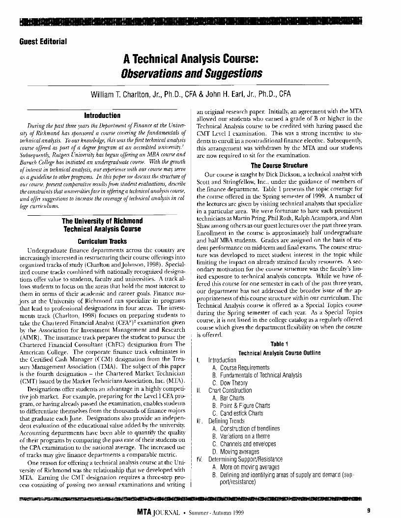
The Course Structure Our course is taught by Dick Dickson, a technical analyst with

Scott and Stringfellow, Inc., under the guidance of members of the finance department. Table 1 presents the topic coverage for the course offered in the Spring semester of 1999. A number of the lectures are given by visiting technical analysts that specialize in a particular area. We were fortunate to have such prominent technicians as Martin Pring, Phil Roth, Ralph Acampora, and Alan Shaw among others as our guest lectures over the past three years. Enrollment in the course is approximately half undergraduate and half MBA students. Grades are assigned on the basis of student performance on mid-term and final exams. The course structure was developed to meet student interest in the topic while limiting the impact on already strained faculty resources. A secondary motivation for the course structure was the faculty’s limited exposure to technical analysis concepts. While we have offered this course for one semester in each of the past three years, our department has not addressed the broader issue of the ap- propriateness of this course structure within our curriculum. The Technical Analysis course is offered as a Special Topics course during the Spring semester of each year. As a Special Topics course, it is not listed in the college catalog as a regularly offered course which gives the department flexibility on when the course is offered.

Table 1

Technical Analysis Course Outline I. Introduction

A. Course Requirements B. Fundamentals of Technical Analysis C. Dow Theory

II. Chart Construction A. Bar Charts B. Point & Figure Charts C. Candlestick Charts

III. Defining Trends A. Construction of trendlines B. Variations on a theme C. Channels and envelopes D. Moving averages

IV. Determining Support/Resistance A. More on moving averages B. Defining and identifying areas of supply and demand (sup-

port/resistance)

MTA JOURNAL * Summer-Autumn 1999 9

C. Defining & identifying areas of accumulation & distribution. D. Money flow analysis

V. Pattern Recognition A. Philosophy of chart patterns: patterning human nature B. Interpretation of chart patterns

VI. Wyckoff Analysis A. A different perspective on interpreting price/volume action. B. General Principles

VIII. Technical Indicators A. Price oscillators B. Trading and money management C. Mechanical trading systems

IX. Sentiment Indicators X. Relative Strength Analysis A. Principles of relative strength B. Intermarket analysis C. Bottom up forecasting

XI. Cycle Theory A. Stock market cycles B. Elliott Wave analysis C. Gann Analysis

XII. Portfolio Management A. Utilizing technical analysis in portfolio management

Two different textbooks have been used in the three semes- ters that the Technical Analysis course has been offered at the Unirersitv of Richmond. The first semester the course was taught, the book’used was Technical Analvsis ExDlained: The Successful Investor’s Guide to SDottinp Investment Turninn Points authored by Martin Pring and published bp McGraw Hill. The last two se- mesters the text has been Technical Analysis of the Futures ,Mar- ket: h ComDrehensire Guide to Trading Methods and Anplica- tions bp John J. Murphy published by the New York Institute of Finance.

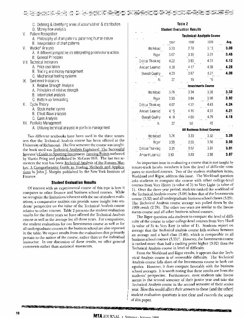
Student Evaluation Results Of interest with an experimental course of this type is how it

compares to other finance and business school courses. MThile we recognize the limitations inherent with the use of student evaluations, a comparative analysis can provide some insight into students’ perspective on the value of the Technical Analysis course relative to other courses. Table 2 presents the student evaluation results for the three years we have offered the Technical Analysis course as well as the average for all three years. For comparison, the student evaluations for our Investments course as well as for all undergraduate courses in the business school are also reported in the table. We report results from the evaluations that primarily pertain to the nature of the course, rather than to the individual instructor. In our discussion of these results, we offer general comments rather than statistical statements.

Table 2

Student Evaluation Results

Technical Analysis Course

Workload

Rigor

Critical Thinking

Amount Learned

Overall Quality

N

1997

3.33

3.67

4.22

4.30

4.23

27

1998 1999

2.78 3.13

3.39 3.31

3.83 4.31

4.17 4.38

3.67 4.27

18 16

Investments Course

Avg.

3.08

3.46

4.12

4.28

4.06

Workload 3.26

Rigor 3.93

Critical Thinking 4.07

Amount Learned 4.15

Overall Quality 4.19

N 27

3.34 3.36

3.84 3.98

4.22 4.43

4.16 4.31

4.00 4.29

50 45

All Business School Courses

3.32

3.92

4.24

4.21

4.16

Workload 3.26 3.30 3.32 3.29

Rigor 3.55 3.55 3.56 3.55

Critical Thinking 3.91 3.92 3.91 3.91

Amount Learned 3.83 3.89 3.88 3.87

An important issue in evaluating a course that is not taught b! tenure-track faculty members is how the level of difficulty compares to standard courses. Tivo of the student evaluation items, M’orkload and Rigor, address this issue. The M’orkload question asks students to compare the course with other college-level courses from 1’ery Hea\? (a value of 5) to Very Light (a value of 1). Over the three year period, students ranked the workload of the Technical Analysis course (3.08) below that of the Investments course (3.32) and all undergraduate business school classes (3.29). The Technical Analysis course average was pulled down by the 1998 result (2.78). The other two years are similar to the Invest- ments course and all other business school courses.

The Rigor question asks students to compare the level of difficulty of the course to other college-level courses from Very Hard (a value of 5) to \‘ery Easy (a value of 1). Students report on average that the Technical analysis course falls midway between an average and a hard class (3.46), which is comparable to all business school courses (3.55) 3. However, the Investments course is ranked more than half a ranking point higher (3.92) than the Technical Analysis course in level of difficulty.

From the Workload and Rigor results, it appears that the Tech- nical Analysis course is of reasonable difficulty. The Technical Analysis course falls short of the Investments course in both cat- egones. However, it does compare favorably with the business school averages. It is worth noting that these results are from the students’ perspective. Furthermore, most students take Invest- ments in the second semester of their junior year and take the Technical Analysis course in the second semester of their senior year. How this would affect their answers to these (and the other) student evaluation questions is not clear and exceeds the scope of this paper.

MTA JOURNAL l Summer-Autumn 1999

The second hvo student evaluation questions reported in Table 2 reflect more favorably on the Technical Analysis course. Stu- dents were asked to rank the amount the course called upon their ability to think critically and analytically from Very Much (a value of 5) to Very Little (a value of 1). For this question, the Technical Analysis course (4.12) ranks similarly to the Investments courses (4.24) and both are notably higher than all undergraduate business school courses (3.91). Students ranking of the amount learned in each course also exhibit a similar relationship. The amount learned in the Technical Analysis course (4.28) is almost identical to the Investments course (4.21) and both are substantially above the business school average (3.87).

The final student evaluation category we report is the student ranking of the overall quality of the course. Students rank the course from Excellent, which has a numerical value of 5, to Poor, which carries a value of 1. This data item is not available for the All Business School Course sample. As the table shows, the Tech- nical Analysis Course (4.06) and the Investments Course (4.16) are viewed by students to be of similar high overall quality.

While our results with the Technical Analysis course have been good, other programs may have difficulty in duplicating our course due to demands on the limited supply of qualified guest lectur- ers. As discussed below, the long-term viability of our program and any new ones will partially depend how this issue is resolved.

The Fundamental Problem A technical analysis course can be taught by existing full-time

college faculty in the finance department or practicing technical analysts acting in a part time or adjunct teaching capacity. Pres- ently, both groups have limitations that bound the number and quality of technical analysis courses that may be offered. At the vast majority of degree granting universities, the primary focus of investments is fundamental analysis. The study of technical analysis is limited to, at most, a single chapter in an investments textbook. Existing finance faculty are either unfamiliar with, and/or skeptical of technical analysis. Thus, their ability and willingness to teach technical analysis topics beyond basic definitions is limited.

Mhile the use of practicing technicians as adjunct faculty addresses the issue of familiarity with technical analysis concepts, professional technicians may not overcome constraints related to accreditation standards. Another problem is that there may not be sufficient availability of practitioners to cover an expanded offering of courses in technical analysis by universities across the country. Furthermore, teaching a semester long course requires a set of organizational and interpersonal skills that are often not inherent to non-faculty professionals.

A key constraint in offering a technical analysis course is finding a qualified and knowledgeable instructor. Full-time faculty are qualified to teach at the university level, but may not have sufficient interest or background in technical analysis concepts. Practicing technicians know the material, but may not be qualified (according to accreditation bodies) or have the skills necessary to teach a college level course. In the sections below, we examine the issues associated with each group in additional de- tail and offer suggestions to address them.

Practitioner Issues

Accreditation The use of practitioners as adjunct faculty is governed by ac-

creditation bodies that oversee universities. Universities are sub ject to accreditation through AACSB (American Association of Colleges and Schools of Business), specifically the standards for accreditation in Business Administration and Accounting. Schools may also be subject to the provisions of a regional accreditation body. The University of Richmond is a member of and subject to the accreditation guidelines of the Southern Association of Col- leges and Schools (SACS).

An overuse of faculty that are not deemed to be “qualified” can endanger a university’s accreditation. In their publication Achieving- Oualitv and Continuous Imnrovement through Self- Evaluation and Peer Review, AACSB states that (page 13) : “ [t] he faculty in aggregate, should have sufficient academic and professional qualifications to accomplish the school’s mission.” Aca- demic qualification is interpreted as a combination of degree completion and post degree activities that maintain the ability to teach in today’s changing environment - research, professional service, and business contacts/relationships. The degree requirements are [l] a doctoral degree in the area of teaching specialization, [2] a doctoral degree in a related business area combined with supplemental preparation in the area of teaching, [3] a doctorate degree outside of business with supplemental preparation in the form of professional development, or [4] substantial coursework in the field of specialization or teaching but no doctoral degree.

The final provision can apply to specialized instructional resources or programs, which might apply to a technical analysis course. In such a case, according to AACSB, the faculty member may have a specialized master’s degree in business, be a current doctoral student, or ABD (all but dissertation completed). These individuals are considered academically qualified but their use should be limited. Under AACSB guidelines, normal academic preparation consists of a minimum of a master’s degree in business and normal professional experience should be relevant to the faculty member’s teaching assignment. Also, “[t] he greater the disparity between the field of academic preparation and the area of teaching, the greater the need for supplemental preparation in the form of professional development.” (page 14).

The Southern Association of Colleges and Schools has separate faculty qualifications for undergraduate and graduate programs. SACS addresses this issue in their publication Criteria for Accreditation (page 44) :

Each full-time and part-time faculty member teaching credit courses leading toward the baccalaureate degree, other than physi- cal education activities courses, must have completed at least 18 graduate semester hours in the teaching discipline and hold at least a master’s degree, or hold the minimum of a master’s degree with a major in the teaching discipline. In exceptional cases, outstand- ing professional experience and demonstrated contributions to the teaching discipline maJ be $n-esented in lieu of foal academic p-ybaration. Such cases must be justified by the institution on an individual basis.

Institutions that offer masters or specialized degrees are held to a higher standard. Each faculty member teaching a master’s degree level course &hold a terminal degree in the teaching field or a related discipline. Terminal degree usually means a doctorate but in some cases a specialized master’s degree, In

MTA JOURNAL * Summer -Autumn 1999 11

unusual cases SACS allows exceptions for faculty members that have exceptional scholarly, creative, or professional experience (i.e. Peter Lynch). An exception may be allowed for a new discipline when there are no faculty members available with academic credentials. In the event of an unusual case, the university must present evidence to justify employment of the faculty member.

How binding the accreditation constraint is varies by university and depends on the accreditation agency(ies) they are governed by, how the rest of their faculty stands in terms of qualifications, and the stage of their accreditation process. In the year the university is being reviewed for accreditation they are likely to follow accreditation guidelines closely.

Most academics lack professional development related to the field of technical analysis, but most practitioners lack the academic qualifications to be certified under accreditation guidelines. Uhile the new discipline exemption may apply to technical analysis, its use depends on a university being willing to apply for and pursue an exemption. Thus, accreditation issues may significantly pre- clude many schools from offering a course in technical analysis.

Availability Even if accreditation requirements do not constitute a binding

constraint, the availability of practitioners may limit the ability of the MTA to stalf college offerings. Teaching a course requires a significant commitment of time with regular and relatively inflex- ible meeting times. Practicing technicians who are subject to rapidly changing demands on their time due to market conditions may find their professional and teaching duties in conflict.

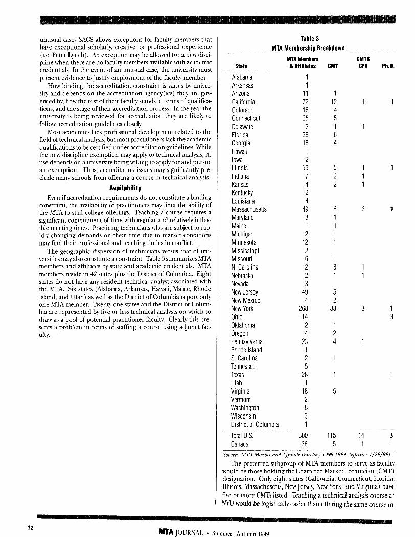
The geographic dispersion of technicians versus that of universities may also constitute a constraint. Table 3 summarizes MTA members and affiliates by state and academic credentials. MTA members reside in 42 states plus the District of Columbia. Eight states do not have any resident technical analyst associated with the MTA. Six states (Alabama, Arkansas, Hawaii, Maine, Rhode Island, and Utah) as well as the District of Columbia report only one MTA member. Twenty-one states and the District of Colum- bia are represented by five or less technical analysts on which to draw as a pool of potential practitioner faculty. Clearly this presents a problem in terms of staffing a course using adjunct faculty.

Table 3

MTA Membership Breakdown

State MTA Members & Aft iliates CMT

CMT& CFA Ph.D.

Alabama 1

Arkansas 1 Arizona 11 California 72 Colorado 16 Connecticut 25 Delaware 3 Florida 36 Georgia 18 Hawaii 1 Iowa 2 Illinois 59 Indiana 7 Kansas 4 Kentucky 2 Louisiana 4 Massachusetts 49 Maryland 8 Maine 1 Michigan 12 Minnesota 12 Mississippi 2 Missouri 6 N. Carolina 12 Nebraska 2 Nevada 3 New Jersey 49 New Mexico 4 New York 268 Ohio 14 Oklahoma 2 Oregon 4 Pennsylvania 23 Rhode Island 1 S. Carolina 2 Tennessee 5 Texas 28 Utah 1 Virginia 18 Vermont 2 Washington 6 Wisconsin 3 District of Columbia 1

1 1

1

1 1 1 1

3 1

1 12 4 5 1 6 4

5 2 2

8 1 1 1 1

1 3 1

5 2

33

1 2 4 1

1

1

5

3 1 3

1

Total U.S. 800 115 14 8 Canada 38 5 1 -

Source: MTA Member and Af,liate Directory 1998-l 999 (effective l/29/99)

The preferred subgroup of MTA members to serve as faculty would be those holding the Chartered Market Technician (CMT) designation. Only eight states (California, Connecticut, Florida, Illinois, Massachusetts, New Jersey, New York, and Virginia) have five or more CMTs listed. Teaching a technical analysis course at NYU would be logistically easier than offering the same course in

MTA JOURNAL l Summer-Autumn 19%

most other states. Fourteen MTA members are listed as holding the combination of a CMT and the fundamental analysis based CFAa designation3, with only Massachusetts (3) and New York (3) reporting more than one. These individuals would be able to teach technical analysis and explain how it relates to and can be used in conjunction with fundamental analysis.

There may be other qualified candidates that are not properly identified in the MTA membership directory. One option to address this issue is to generate a database of academically qualified technicians and assure that the information is current. Addition- ally, it may be possible to have the CMT designation certified as a specialized designation/degree that qualifies the holder to teach the course in technical analysis. AACSB holds that a JD degree constitutes a terminal degree for individuals teaching business law or legal environment courses. An LLM in taxation or a CPA combined with a master’s degree in accounting is considered a terminal degree for accounting/tax courses. While this course of action would likely be a longer-term solution, it may warrant further investigation.

The ideal combination for teaching technical analysis would be a person who holds both a business doctorate and the CMT designation. Table 3 lists eight MTA members as holding Ph.D.s. However, none hold the combination of a Ph.D. and the CMT designation. Thus, the number of potentially academically qualified technical analysts is severely limited and geographically con- centrated. One solution, albeit an unlikely one, is to have existing CMT obtain Ph.D.s from accredited universities. Given the opportunity cost and length of time necessary to obtain a Ph.D., it seems unlikely that this would be a viable solution for the majority of practicing technicians. The alternative solution is for existing Ph.D.s to obtain CMT?. We address this approach in the following sections.

Faculty Issues

Awareness and Promotion of the CMT The CMT is one of a growing number of professional designa-

tions that competes for acceptance with the other established industry credentialing organizations. The CFA has over 25,000 charterholders as compared to the several hundred CMT desig- nees. If one goal of the MTA is to promote the CMT and expand the number of people sitting for the exams, it could begin a cam- paign to increase awareness of the program. The MTA can begin to fill the void of Ph.D.s holding the CMT designation by educat- ing academics as to the value of and requirements for the designation. A good first step for improving the likelihood that existing Ph.D.s would pursue the CMT designation is exposure to technical analysis through seminars, professional exposure (internships) and research opportunities. Something as simple as educator discounts for registration for the exams may encourage finance academics to earn their CMT designation. Other designations, such as the CFA, have had similar programs for a number of years and have seen a marked increase in academic participation.

Two organizations can serve as examples for comprehensive programs for increasing awareness. The Treasury Management Association (issuer of the CCM designation) has begun a program that focuses on increasing academic support of the designation. In April, 1999, the TMA sent a two-page academic information request form to university faculty. The letter was addressed Dear Professor and starts off Teaching! Research! Service! These are the criteria on which faculty are evaluated which makes them key

issues for almost university professor. The letter explains how the TMA and the CCM can assist faculty in these critical areas. As part of this program, the TMA will announce a major new program of financial support for academic research in October. To encourage faculty participation at their annual Treasury Manage- ment Conference, the TMA offers a 75% academic discount. Also, to increase student awareness ofjob opportunities related to Cash Management, the TMA provides free copies of a Treasury Man- agement Careers brochure as well as information on the CCM designation.

While the Chicago Board Options Exchange (CBOE) does not offer a professional designation, it has taken an active role in pro- moting the use and understanding of options. The Options In- stitute was designed to bridge the gap between theory and practice and between academics and practitioners. It offers a comprehensive curriculum taught by industry professionals that cov- ers the theory, strategy and trading techniques employed in the options markets. Programs are offered in Chicago and around the nation to academics, industry participants, and the public. Also, the CBOE offers a two-day seminars for academics that focuses on teaching applications and research opportunities related to options. Professors are regularly invited to the free seminar.

The MTA can combine aspects of the TMA and CBOE approaches and design an education program to increase awareness and acceptance of technical analysis and the CMT designation. A Technical Analysis Institute could provide the forum to teach academics to understand and teach technical analysis at their universities. One of the most important ways for the MTA to increase academic interest in technical analysis issues is through the encouragement and sponsorship of academic research. We discuss this issue in the following section. Following that, we discuss ways to encourage the teaching of technical analysis courses.

Academic Research Of the three components most faculty are evaluated on (re-

search, teaching, and service), research is often the most difficult of the three in which to achieve success. For this and other reasons, it is often valued as the most important component. Any way in which the MTA can help academics achieve additional publications would most likely be viewed positively by academics. This could lead to an increase in the amount of technical analysis based academic research. The two main areas where research assistance is most valuable are in helping to get a project off the ground and in increasing the outlets for working projects. We discuss each below.

Most current academics are relatively unfamiliar with technical analysis and, as a result, it may be difficult for them to generate sufficient potential research ideas. The MTA could provide a valuable service by developing connections between practitioners and academics and encouraging practitioners to use their expertise in assisting academicians. The aforementioned Technical Institute would be a good forum for the development of these relationships. Another important issue for academic research is the availability of good data. Most academics have ready access to U.S. stock market data. However, many do not have good access to foreign market data or commodity pricing. Thus, the Institute could also act as a warehouse of datasets commonly used by technical analysts. One usual difference between practitioner (of any type) and academic research is that academics tend to use more historical data whereas practitioners are generally more focused on recent market conditions. A final suggestion is for the establishment of research grants which would encourage academics to start projects.

MTA JOURIUL * Summer-Autumn I999 13

The MTA could also play an important role on the output side of the research pipeline. Competitive monetary research awards are a good way to encourage additional research. There are non- monetary methods of encouragement as well. While not equivalent to a publication, most universities view presenting a paper at a conference as evidence of active scholarship. Paper sessions, or tracks, focusing on technical analysis issues at the conferences are a means for professors to receive acknowledgment for their work. These sessions could be held at the national and/or regional conferences.

Ultimately what counts are the articles a professor publishes. For most professors, the minimum requirement is that an article be published in a refereed journal. Beyond this exists a relative ranking ofjournals based on their selectivity and the esteem the journal is held in by the profession. The more journals that are available to publish technical analysis articles, and the better these journal are viewed, the more desirable a publication in them will be to a professor.

Textbooks For many professors, teaching is second to research in its im-

portance, for others it is of primary importance. Several impedi- ments currently exist to teaching a technical analysis course beyond the limitation already discussed above. Perhaps the most significant non-staffing issue is the lack of an adequate technical analysis textbook. Both books used in our course (the Pring and Murphy books) are written for practitioners and do not qualify as academic textbooks. Murphy’s text is narrowly focused on the futures market and is dated (it was published in 1986)j. Both books’ format is consistent with their intended audience - practitioners. Their intent is to familiarize readers with technical analysis concepts. Each chapter consists of text ending in a one paragraph conclusion and/or summary.

A book which can serve as a good example of an academic textbook is Investment Analvsis and Portfolio Management by Frank Reilly and Keith Brown. This textbook is commonly used in Investments and Portfolio Management/Security Analysis courses and is required reading for CFA candidates. It combines academic theory and CFA based practical applicatio&. Each chapter begins with a bulleted list of learning objectives that focus the reader on the main points prior to reading the chapter. Also, each chapter ends with a summary followed by a set of short answer questions and a set of problems that allow the student to assess their grasp of the concepts covered in the chapter. A number of the questions and problems are accompanied by a CFA trademark indicating that the question has appeared on a prior CFA examination. A reference section is included in each chapter which guides the reader to sources where additional information can be obtained. While the content of the books vary, most textbooks follow a format similar to the one described above.

Supplemental Materials Academic textbooks are accompanied by a seemingly endless

supply of ancillary materials designed to either help instructors prepare their lectures or students study the material covered in the course. These materials are especially important when a new subject area is being prepped for instruction. A typical set of supplemental materials are those included with Fundamentals of Financial Management by Brigham and Houston. This textbook is widely used and has been adopted by hundreds of universities for their introductory corporate finance course.

We first discuss the materials developed for students, A study

guide is sold to students separately or can be included as a package with the textbook. The study guide provides summaries of the main concepts in each chapter combined with focused questions and problems designed to provide feedback to the students. Problems are usually in a multiple-choice format. The study guide provides structure and pre-examination evaluation to the participants.

Blueprints are an additional learning aid designed to help students take better notes in class. Students often have to choose between taking notes and listening to the points discussed in class. Blueprints provide students a hard copy and overview of the material covered by the instructor. Students can augment the general notes during or after the lecture period. Instructors can modify the blueprints and use them as their lecture notes. The blueprints, a syllabus, and other related materials can be provided to students at the beginning of the semester in a “course pack” available for purchase through the university bookstore.

The authors provide extensive support to professors. Inte- grated cases and presentation software are provided to augment end of chapter problems. These minicases cover the key topics in each chapter in a systematic manner. The cases are designed to focus the students’ attention and allow the instructor to design the lecture material around the case. A set of electronic slides or PowerPoint presentation based on the cases is included. The PowerPoint presentation allows slides to be developed in layers, building a presentation one piece at a time compared to “static” overhead transparencies. The combination of case studies and presentation software is particularly useful for inexperienced teachers or experienced teachers teaching a new course.

Videos covering key financial concepts are also included in the supplemental materials. The authors provide fourteen short videotapes which can be used to introduce various topics. Videos could be a particularly effective tool for teaching technical analysis. A library.of in-depth videos could be produced covering the more specialized concepts of techniques included in a technical analysis textbook. For example, candlesticks, sentiment indicators, point and figure charts or other subjects could be presented by the leading experts in each area. Fundamental based finance academics may not be comfortable teaching these areas and the assistance of a guest speaker or a video could prove valuable. The previously discussed limitations on guest speakers could make videos an especially attractive alternative. Videos would be most effective if developed specifically for an academic audience rather than edited from a presentation to practitioners. Videocon- ferences could provide an alternative to videos or can be used in conjunction with the video to provide a question and answer ses- sion for students. However, the limited availability of teleconfer- ence facilities on campuses and their relative high cost might con- strain this approach. of this type. The tremendous pace of development of other distance learning technologies may offer additional capabilities in the near future which could lower the cost hurdle.

Some of the end of the chapter problems in the Brigham and Houston textbook are designed to require the use of a spreadsheet template to solve. A computer problem diskette is provided with the textbook that contains the spreadsheet templates (usually in LOTUS l-2-3 or Microsoft Excel format). The templates are stand alone programs and no knowledge of the underlying spreadsheet programs is required. In theory, hands-on application reinforces classroom discussion which improves learning. A technical analysis data disk could include time-series market data

14 MTA JOURNAL * Summer -Autumn 1999

and charts which would allow students to apply the techniques they learn in class on historical and/or current sets of financial data. The quantitative nature of technical analysis makes this approach especially appealing.

A test bank is provided to the instructor in book form and as a computer software program. Questions are in multiple choice formats and the software allows for the construction of custom- ized and random examinations. If the instructor prefers essay and non multiple-choice problems, the questions in the test bank can provide a starting point.

The instructor’s manual is the most important of the supplemental textbook materials. Brigham and Houston include a sample syllabus covering course objectives, class procedures, examination and grading policies, and required materials. Course schedules are provided for a two-day a week (Tuesday and Thurs- day) and three-day a week (Monday, Wednesday, and Friday) teaching format that specifies the chapter and the topic for each class period. An examination schedule is also included in the course schedule. These are illustrative but provide valuable guidance to an instructor teaching a new course for the first time. The sample syllabus and course schedule would be invaluable additions to an instructor’s manual accompanying the technical analysis textbook. For each chapter the following is provided: An overview and learning objectives, lecture suggestions, answers to the end of chapter problems, and the solution to the integrated case. Answers to the even numbered questions are often include in the textbook itself, while the answers to the odd numbered questions are given only in the instructor’s manual.

The MTA could design an academic textbook that follows the format described above while incorporating the major tenets stressed in the CMT examination. Some possible unifying themes for a textbook are given in Table 4 which was derived from MTA members descriptions of themselves. The construction of a textbook could also have other beneficial uses. It could serve as a valuable vehicle for the MTA to articulate the body of knowledge required for the CMT designation.

As discussed, the supplemental materials are often a critical factor in the adoption of a textbook and should be an integral part of the textbook development process. This is especially true given the current acceptance level of technical analysis by professors and their relative inexperience teaching the material. The first step in the textbook process is to agree upon a curriculum. After that, an author and an editor are selected at which point chapters could be assigned to the leading expert in each area. Writing an academic textbook, in conjunction with the necessar) supplemental materials, is a vital step in moving technical analysis toward the mainstream of finance curriculum at the university level.

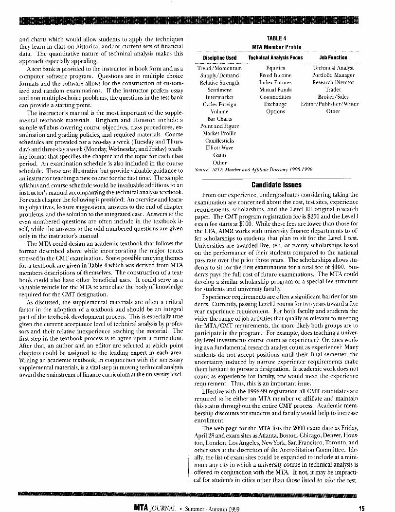
TABLE 4

MTA Member Profile

Discipline Used Technical Analysis Focus Job Function

Trend/Momentum Equities Technical Analyst Supply/Demand Fixed Income Portfolio Manager Relative Strength Index Futures Research Director

Sentiment .Mutual Funds Trader Intermarket Commodities Broker/Sales

Cycles Foreign Exchange Editor/Publisher/Writer Volume Options Other

Bar Charts Point and Figure Market Profile Candlesticks Elliott Wave

Gann Other

Source: MTA LKmber and Affiliate Directq 1998-l 999

Candidate Issues From our experience, undergraduates considering taking the

examination are concerned about the cost, test sites, experience requirements, scholarships, and the Level III original research paper. The CMT program registration fee is $250 and the Level I exam fee starts at $100. While these fees are lower than those for the CFA, AIMR works with university finance departments to offer scholarships to students that plan to sit for the Level I test. Universities are awarded five, ten, or twenty scholarships based on the performance of their students compared to the national pass rate over the prior three years. The scholarships allows students to sit for the first examination for a total fee of $100. Stu- dents pays the full cost of future examinations. The MTA could develop a similar scholarship program or a special fee structure for students and university faculty.

Experience requirements are often a significant barrier for students. Currently, passing Level I counts for two years toward a five year experience requirement. For both faculty and students the wider the range ofjob activities that qualify as relevant to meeting the MTA/CMT requirements, the more likely both groups are to participate in the program. For example, does teaching a university level investments course count as experience? Or, does working as a fundamental research analyst count as experience? Man) students do not accept positions until their final semester, the uncertainty induced by narrow experience requirements make them hesitant to pursue a designation. If academic work does not count as experience for faculty, few would meet the experience requirement. Thus, this is an important issue.

Effective with the 1998-99 registration all CMT candidates are required to be either an MTA member or affiliate and maintain this status throughout the entire CMT process. Academic membership discounts for students and faculty would help to increase enrollment.

The web page for the MTA lists the 2000 exam date as Friday, April 28 and exam sites as Atlanta, Boston, Chicago, Denver, Hous- ton, London, Los Angeles, NewYork, San Francisco, Toronto, and other sites at the discretion of the Accreditation Committee. Ide- ally, the list of exam sites could be expanded to include at a minimum any city in which a university course in technical analysis is offered in conjunction with the MTA. If not, it may be impracti- cal for students in cities other than those listed to take the test.

MTA JOURML * Summer -Autumn 1999 15

This would probably limit the availability of technical analysis courses to those universities located near a test site.

Finally, the requirement at Level III to write a research paper approved by the Accreditation Committee creates a logistical bottleneck to expansion of the designation. The number of qualified reviewers to read and approve the manuscripts limits the ability to promote the CMT as a mass appeal designation. Proposals to replace the research report with an examination are under consideration by the MTA. If approved a major hurdle will be removed.

Conclusion In general, our experience with the Technical Analysis course

has been positive. Student demand for the course is steady and we expect student interest to remain at its current level for some time to come. The student evaluation results are good with the Technical Analysis course achieving scores comparable to or better than the average undergraduate business school course. Also, the difficulty of the course meets our expectations for a finance course taught by non-tenure track faculty. At some point, our department may have to address the issue of how this course fits into our curriculum. However, we expect to continue to offer the course in its current form. The ability of other universities to offer similar programs is currently limited by the availability of qualified teachers. While the suggestions offered above do not constitute a comprehensive set of all of the relevant issues, ad- dressing them would lower the hurdles that interested schools currently face. The lower the barriers are, the more likely it is that universities will consider initiating academic coverage of technical analysis.

References Achieving Oualitv and Continuous Imorovement through Self- Evaluation and Peer Review, Standards for Accreditation Busi- ness Administration and Accounting, American Association of Colleges and Schools of Business 19941995 Criteria for Accreditation, Southern Association of Colleges and Schools, Commission on Colleges, 1995, Ninth Edition MTA Member and Affiliate Directorv 1998-1999, Market Tech- nicians Association, Inc. Brigham, Eugene F., and Joel E Houston, Fundamentals of Financial Management, Eighth Edition, 1998, The Dryden Press Charlton, William T. Jr., Course Tracking Along Professional Des- ignations: The CXA Track, August 1998, Financial Practice and Education 8 (No.1, Spring/Summer), 69-82 Charlton, William T. Jr., and Robert Johnson, The CE4 Designa- tion and the Finance Curriculum: A Survq of Faculty, forthcom- ing, Journal of Financial Education. Murphy, John J., Technical Analysis of the Futures Market: A Comnrehensive Guide to Trading Methods and Anolications, New York Institute of Finance, 1986 Murphy, John J., Technical Analysis of the Financial Markets: A Comorehensive Guide to Trading Methods and Anolications, New York Institute of Finance, 1999

q Pring, Martin J., Technical Analvsis Exolained: The Successful Investor’s Guide to Sootting Investment Turning Points, Third Edition, 1991, McGraw-Hill

q Reilly, Frank K. and Keith C. Brown, Investment Analvsis and Portfolio Management, Fifth Edition, 1997, The Dryden Press

Endnotes ’ Prior to the inauguration of our course, Henry Pruden of-

fered a technical analysis course at Golden Gate University. How- ever, the course was offered in the continuing education program rather than as part of the regular curriculum.

* CFA@ is a registered trademark of the Institute of Chartered Financial Analysts, licensed to the Association for Investment Management and Research.

3That the average level of difficulty for all business school is above the average ranking has at least two explanations. First, students may over estimate the difficulty of a course and thereby induce an upward bias. The evaluation form asks respondents to rank the course versus other college-level courses. Therefore, a second reason may be that business school classes are harder than the courses the students take prior to entering the business school. These two possibilities are not mutually exclusive, so both may be present in the sample.

‘The use of distance learning technology may also be a solution to this problem. However, it would most likely only be a partial solution. While it might solve the geographical limitation, accreditation issues remain unresolved. Thus, distance learning technology may be an excellent support tool but not a primary means of offering a course for college credit.

5A newer version of Murphy’s text entitled Technical Analvsis of the Financial Markets has recently been released. Reportedly, it has a greater focus on equity markets. We have not reviewed a copy of the new text, so our comments focus on the previous version of the book.

6 Ironically, this text, like most fundamental based textbooks, has the obligatory chapter on technical analysis.

William Charlton, Ph.D. &John Earl, Ph.D.

William T. Charlton, Jr., Ph.D., CFA, is an assistant professor of finance at the E.C. Robins School of Business at the University of Richmond. He teaches corporate finance and investments as well as acting as the faculty advisor for the CFA Track and the University of Richmond Student Man- aged Investment Fund (known as the Spider Fund). He holds a bachelors of science in electrical engineering from Texas A&M University, an MBA from St. Mary’s University (San Antonio, Texas), and a Ph.D. in finance from the University of Texas at Austin. Prior to entering the Ph.D. program, he worked for Hewlett Packard for five years as a computer field engineer.

John H. Earl, Jr. Ph.D., is an associate professor of finance at the E.C. Robins School of Business at the University of Richmond. He teaches corporate finance, investments and portfolio management/security analysis at both the undergraduate and graduate levels. John holds bachelors and master’s degrees in finance from the University of Massachu- setts and a Ph.D. in finance from Arizona State University. In addition he holds the CFA, CLU, ChFC, CIC, CFP, and ARM designations.

MTA JOURNAL * Summer-Autumn 1999

A Composite Indicator Using Momentum and Trend Following Components Provides Early Identification of

Turning Points in S&P 500

James E. Young

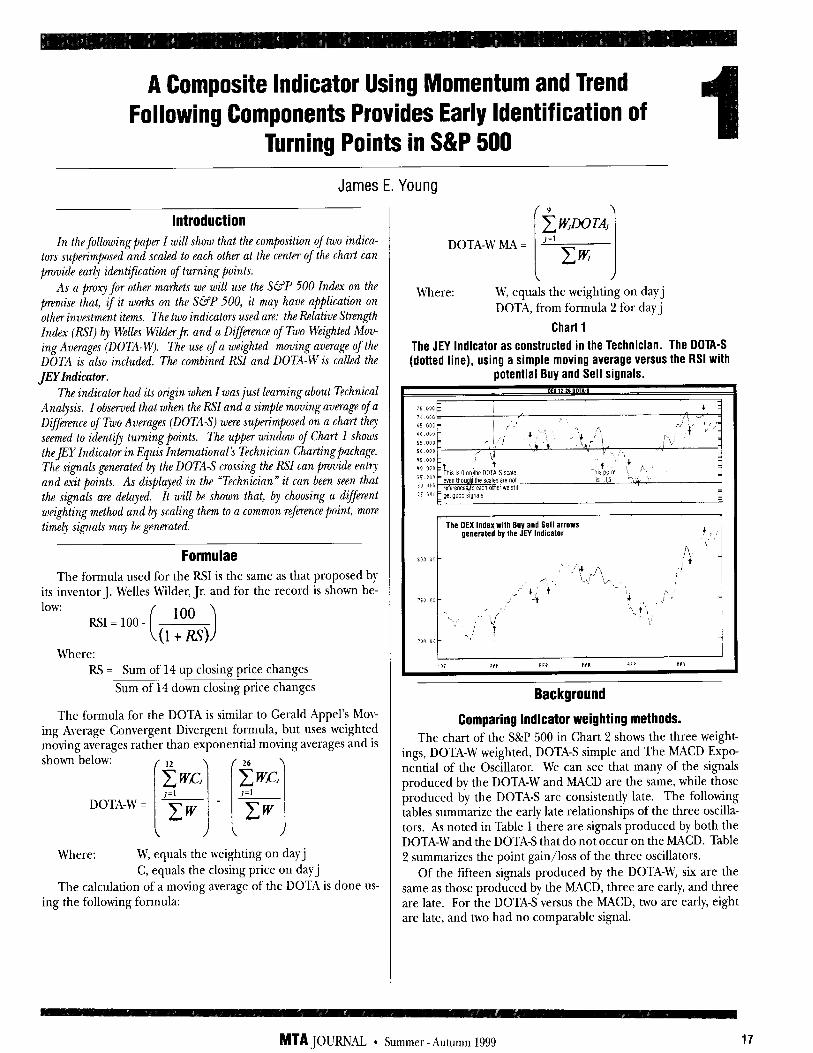
Introduction In the following paper I will show that the composition of two indica-

tors superimposed and scaled to each other at the center of the chart can provide early identification of turning points.

As a proxy for other markets we will use the S&P 500 Index on the premise that, if it works on the S&P 500, it may have application on other investment items. The two indicators used are: the Relative Strength Index (RX) by Welles Wilder Jr. and a DifIfmence of Two Weighted Mov- ing Averages (DOTA-W). The use of a weighted moving average of the DOTA is also included. The combined RSI and DOTA-W is called the JEYIndicator.

The indicator had its origin when I was just learning about Technical Analyis. I observed that when the RSI and a simple moving average of a Difference of Two Averages (DOTA-S) were superimposed on a chart thq

seemed to identify turning points. The upPer window of Chart 1 shows theJEY Indicator in Equis International’s Technician Charting package. The signals generated @ the DOTAS crossing the RSI can @nG’e entv and exit points. As displayed in the “Technician” it can been seen that the signals are delayed. It will be shown that, by choosing a different weighting method and bJ scaling them to a common reference point, more time4 signals may be generated.

Formulae The formula used for the R!3 is the same as that proposed by

its inventor J. Welles Wilder, Jr. and for the record is shown below:

RSI = 100 - 100

( ) o+m Where:

RS = Sum of 14 up closing price changes Sum of 14 down closing price changes

The formula for the DOTA is similar to Gerald Appel’s Mov- ing Average Convergent Divergent formula, but uses weighted moving averages rather than exponential moving averages and is shown below: / I2 \ /26 \

cwc, CWCJ ]=l ]=I

DOTA-W = ~ - p cw

! I( ) Where: W, equals the weighting on day j

C, equals the closing price on day j The calculation of a moving average of the DOTA is done us-

ing the following formula:

Where: W, equals the weighting on day j DOTA, from formula 2 for day j

Chart 1

The JEY Indicator as constructed in the Technician. The DDTA-S (dotted line), using a simple moving average versus the RSI with

potential Buy and Sell signals.

The OEX lnde: with Buy and Sell arrows generated by the JEY Indicator

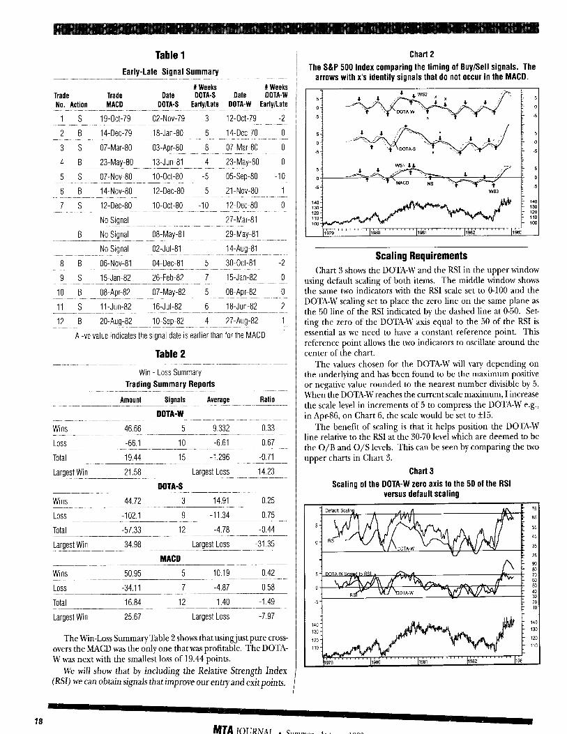
The chart of the S&P 500 in Chart 2 shows the three weight- ings, DOTA-W weighted, DOTA-S simple and The MACD Expo- nential of the Oscillator. We can see that many of the signals produced by the DOTA-W and MACD are the same, while those produced by the DOTA-S are consistently late. The following tables summarize the early late relationships of the three oscillators. As noted in Table 1 there are signals produced by both the DOTA-W and the DOTA-S that do not occur on the MACD. Table 2 summarizes the point gain/loss of the three oscillators.

Of the ftiteen signals produced by the DOTA-W, six are the same as those produced by the MACD, three are early, and three are late. For the DOTA-S versus the MACD, two are early, eight are late, and two had no comparable signal.

Background

Comparing Indicator weighting methods.

MTA JOURhN * Summer-Autumn 1999 17

18

Table 1

Early-Late Signal Summary - -~ ..- -- #Weeks #Weeks

Trade Trade Date DDTA-S Date DDTA-W No. Action MACD DDTA-S Early/Late DDTA-W Early/Late

1 s 19-act-79 02-Nov-79 3 12-act-79 -2

2 B 14-Dee-79 18-Jan-80 6 14-Dec.70 0

3 s 07-Mar-80 03.Apr-80 8 07-Mar-80 0

4 B 23-May-80 13-Jun-81 4 23-May-80 0

5 s 07-Nov-80 1 O-0&80 -5 05-Sep-80 -10

6 B 14-Nov-80 12-Dec.80 5 21-Nov-80 1

7 s 12-Dee-80 1 O-Ott-80 -10 12.Dee-80 0

No Signal 27-Mar-81

B No Signal 08-May-81 29.May-81

No Signal 02-J&81 14-Aug-81 .~. .-----. --- .~ ~~ 8 B 06.Nov-81 04-Dee-81 5 30.Ott-81 -2

9 s 15.Jan-82 26-Feb-82 7 15.Jan-82 0

10 B 08-Apr-82 07-May-82 5 08.Apr-82 0

11 s ll-Jun-82 16-Jul-82 6 18-Jun-82 2

12 B 20.Aug-82 1 O-Sep-82 4 27.Aug-82 1

A -ve value indicates the signal date is earlier than for the MACD

Table 2

Win - Loss Summary Trading Summary Reports

Amount Signals Average Ratio

DOTA-W

Wins 46.66 5 9.332 0.33

Loss -66.1 10 -6.61 0.67

Total -19.44 15 -1.296 -0.71 - Largest Win 21.58 Largest Loss -14.23 _ --~- ~.~ ~-~----

DDTA-S

Wins 44.72 3 14.91 0.25 ~- Loss -102.1 9 -11.34 0.75

Total -57.33 12 -4.78 -0.44

Largest Win 34.98 Largest Loss -31.35

MACD

Wins 50.95 5 10.19 0.42

Loss -34.11 7 -4.87 0.58

Total 16.84 12 1.40 -1.49

Largest Win 25.67 Largest Loss -7.97

The Win-Loss Summary Table 2 shows that usingjust pure crossovers the h4ACD was the only one that was profitable. The DOTA- W was next with the smallest loss of 19.44 points.

We will show that by including the Relative Strength Index PSI) we can obtain signals that improve our entry and exitpoints.

I

Chart 2

The S&P 500 Index comparing the timing of Buy/Sell signals. The arrows with x’s identify signals that do not occur in the MACD.

Scaling Requirements Chart 3 shows the DOTA-W and the RSI in the upper window

using default scaling of both items. The middle window shows the same two indicators with the RSI scale set to O-100 and the DOTA-W scaling set to place the zero line on the same plane as the 50 line of the RSI indicated by the dashed line at O-50. Set- ting the zero of the DOTA-W axis equal to the 50 of the RSI is essential as we need to have a constant reference point. This reference point allows the two indicators to oscillate around the center of the chart.

The values chosen for the DOTA-W will vary depending on the underlying and has been found to be the maximum positive or negative value rounded to the nearest number divisible by 5. When the DOTA-Wreathes the current scale maximum, I increase the scale level in increments of 5 to compress the DOTA-W e.g., in Apr-86, on Chart 6, the scale would be set to f15.

The benefit of scaling is that it helps position the DOTA-W line relative to the RSI at the 30-70 level which are deemed to be the O/B and O/S levels. This can be seen by comparing the two upper charts in Chart 3.

Chart 3

Scaling of the DOTA-W zero axis to the 50 of the RSI versus default scaling

c I

MTAJOLXNAL * Summer - htllmn IQQO

Relative Strength Characteristics The RSI is a momentum indicator and depends solely on

changes in closing prices. It always provides leading or comci- dent signals. The double use of ratios makes the RSI subject to greater volatility, distortion, and erratic movement. The RSI has six major Interpretive Factors. In the list below the first five were by its developer J. Welles Wilder’ and the sixth by the research team of Colby and Myers’. The number in parentheses following each factor identifies its order of significance.

ke&nce between Price and the RSI (1) Tops/Bottoms at 70/30 (1)

The Failure Swing (2) ~- Chart Formations (3)

--- Support and Resistance (4) Reversals of the RSI at 50 (5)

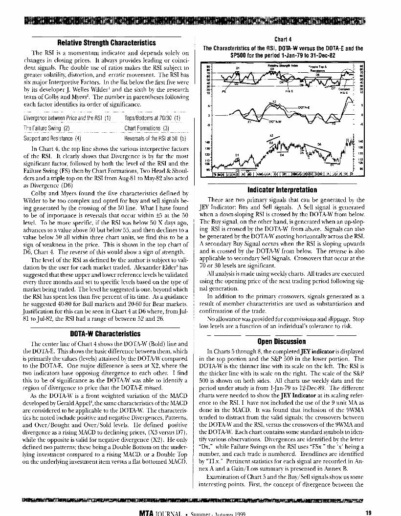
In Chart 4, the top line shows the various interpretive factors of the RSI. It clearly shows that Divergence is by far the most significant factor, followed by both the level of the RSI and the Failure Swing (FS) then by Chart Formations, TNTO Head & Shoul- ders and a triple top on the RSI from Aug-81 to May-82 also acted as Divergence (D6)

Colby and Myers found the fire characteristics defined by Wilder to be too complex and opted for buy and sell signals being generated by the crossing of the 50 line. What I have found to be of importance is reversals that occur within +5 at the 50 level. To be more specific, if the RSI was below 50 X days ago, advances to a value above 50 but below 55, and then declines to a value below 50 all within three chart units, we find this to be a sign of weakness in the price. This is shown in the top chart of D6, Chart 4. The reverse of this would show a sign of strength.

The level of the RSI as defined by the author is subject to vali- dation by the user for each market traded. Alexander Eldeti has suggested that these upper and lower reference levels be validated every three months and set to specific levels based on the type of market being traded. The level he suggested is one, beyond which the RSI has spent less than five percent of its time. As a guidance he suggested 40-80 for Bull markets and 20-60 for Bear markets. Justification for this can be seen in Chart 4 at D6 where, from Jul- 81 to Jul-82, the RSI had a range of between 52 and 26.

DOTA-W Characteristics The center line of Chart 4 shows the DOTA-W (Bold) line and

the DOTA-E. This shows the basic difference between them, which is primarily the values (levels) attained bv the DOTA-W compared to the DOTA-E. One major difference’is seen at X2, where the two indicators have opposing divergence to each other. I find this to be of significance as the DOTA-W was able to identify a region of divergence to price that the DOTA-E missed.

As the DOTA-W is a front weighted variation of the MACD developed by Gerald Appel’, the same characteristics of the MACD are considered to be applicable to the DOTA-U’. The characteristics he noted include positive and negative Divergences, Patterns, and Over/Bought and Over/Sold levels. He defined positive divergence as a rising MACD to declining prices, (X3 versus D7), while the opposite is valid for negative divergence (X2). He only defined two patterns; these being a Double Bottom on the underlying investment compared to a rising ,MACD, or a Double Top on the underlying investment item versus a flat bottomed MACD.

Chart 4

The Characteristics of the RSI, DDlA-W versus the DDTA-E and the SP500 for the period l-Jan-79 to 31-Dee-82

Indicator Interpretation There are two primary signals that can be generated by the

JEY Indicator: Buy and Sell signals. A Sell signal is generated when a down-sloping RSI is crossed by the DOTA-W from below. The Buy signal, on the other hand, is generated when an up-sloping RSI is crossed by the DOTA-W from above. Signals can also be generated by the DOTA-W moving horizontally across the RSI. A secondary Buy Signal occurs when the RSI is sloping upwards and is crossed by the DOTA-W from below. The reverse is also applicable to secondary Sell Signals. Crossovers that occur at the 70 or 30 levels are significant.

All analysis is made using weekly charts. All trades are executed using the opening price of the next trading period following signal generation.

In addition to the primary crossovers, signals generated as a result of member characteristics are used as substantiation and confirmation of the trade.

No allowance was provided for commissions and slippage. Stop loss levels are a function of an individual’s tolerance to risk.

Open Discussion In Charts 5 through 8, the completed JEY indicator is displayed

in the top portion and the S&P 500 in the lower portion. The DOTA-W is the thinner line with its scale on the left. The RSI is the thicker line with its scale on the right. The scale of the S&P 500 is shown on both sides. All charts use weekly data and the period under study is from l-Jan-79 to 12-Dee-89. The different charts were needed to show the JEY Indicator at its scaling reference to the RSI. I have not included the use of the 9 unit MA as done in the MACD. It was found that inclusion of the 9NWA tended to distract from the valid signals; the crossovers between the DOTA-M’ and the RSI, v-ersus the crossovers of the 9MMA and the DOTA-W. Each chart contains some standard symbols to identify various observations. Divergences are identified bv the letter “Dx,” while Failure Swings on the RSI uses “FSx n the “x’ being a number, and each trade is numbered. Trendlines are identified by “TLx.” Pertinent statistics for each signal are recorded in An- nex A and a Gain/Loss summary is presented in Annex B.

Examination of Chart 5 and the Buy/Sell signals show us some interesting points. First, the concept of divergence between the

MTA JOURML l Summer - Autumn 1999 19

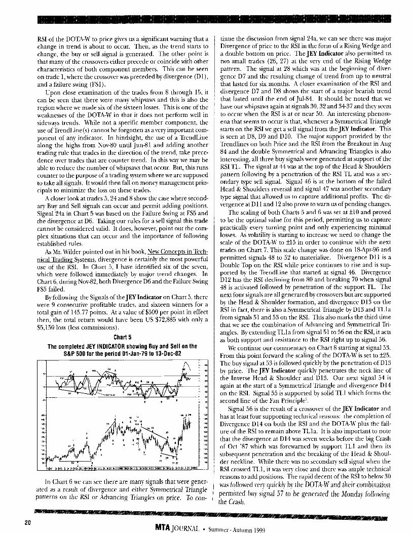
RSI of the DOTA-W to price gives us a significant warning that a change in trend is about to occur. Then, as the trend starts to change, the buy or sell signal is generated. The other point is that many of the crossovers either precede or coincide with other characteristics of both component members. This can be seen on trade 1, where the crossover was preceded by divergence (D 1)) and a failure swing (FSl).

Upon close examination of the trades from 8 through 15, it can be seen that there were many whipsaws and this is also the region where we made six of the sixteen losses. This is one of the weaknesses of the DOTA-W in that it does not perform well in sideways trends. While not a specific member component, the use of TrendLine cannot be forgotten as a very important component of any indicator. In hindsight, the use of a TrendLine along the highs from Nov-80 until Jun-81 and adding another trading rule that trades in the direction of the trend, take prece- dence over trades that are counter trend. In this way we may be able to reduce the number of whipsaws that occur. But, this runs counter to the purpose of a trading system where we are supposed to take all signals. It would then fall on money management prin- cipals to minimize the loss on these trades.

A closer look at trades 5,24 and 8 show the case where secondary Buy and Sell signals can occur and permit adding positions. Signal 24a in Chart 5 was based on the Failure Swing at FS5 and the divergence at D6. Taking our rules for a sell signal this trade cannot be considered valid. It does, however, point out the complex situations that can occur and the importance of following established rules.

As Mr. Wilder pointed out in his book, New Concents in Tech- nical Trading Svstems, divergence is certainly the most powerful use of the RSI. In Chart 5, I have identified six of the seven, which were followed immediately by major trend changes. In Chart 6, during No\r-82, both Divergence D6 and the Failure Swing FS5 failed.

By following the Signals of the JEY Indicator on Chart 5, there were 9 consecutive profitable trades, and sixteen winners for a total gain of 145.77 points. At a value of $500 per point in effect then, the total return would have been US $72,885 with only a $5,150 loss (less commissions).

Chart 5

The completed JEY INDICATOR showing Buy and Sell on the S&P 500 for the period Ol-Jan-79 to 13-Dee-82

In Chart 6 we can see there are many signals that were generated as a result of divergence and either Symmetrical Triangle patterns on the RSI or Advancing Triangles on price. To con-

tinue the discussion from signal 24a, we can see there was major Divergence of price to the RSI in the form of a Rising Wedge and a double bottom on price. The JEY Indicator also permitted us hvo small trades (26, 27) at the very end of the Rising Wedge pattern. The signal at 28 which was at the beginning of divergence D7 and the resulting change of trend from up to neutral that lasted for six months. A closer examination of the RSI and divergence D7 and D8 shows the start of a major bearish trend that lasted until the end of Jul-84. It should be noted that we have our whipsaws again at signals 30,32 and 3437 and they seem to occur when the RSI is at or near 50. An interesting phenomena that seems to occur is that, whenever a Symmetrical Triangle starts on the RSI we get a sell signal from the JEY Indicator. This is seen at D8, D9 and DlO. The major support provided by the Trendlines on both Price and the RSI from the Breakout in Aug 84 and the double Symmetrical and Advancing Triangles is also interesting, all three buy signals were generated at support of the RSI TL. The signal at 44 was at the top of the Head & Shoulders pattern following by a penetration of the RSI TL and was a secondary type sell signal. Signal 46 is at the bottom of the failed Head & Shoulders reversal and signal 47 was another secondary type signal that 11 a owed us to capture additional profits. The divergence at Dll and 12 also prove to warn us of pending changes.

The scaling of both Charts 5 and 6 was set at f10 and proved to be the optimal value for this period, permitting us to capture practically every turning point and only experiencing minimal losses. As volatility is starting to increase we need to change the scale of the DOTA-W to f15 in order to continue with the next trades on Chart 7. This scale change was done on 18-Apr-96 and permitted signals 48 to 52 to materialize. Divergence Dll is a Double Top on the RSI while price continues to rise and is supported by the TrendLine that started at signal 46. Divergence D12 has the RSI declining from 80 and breaking 70 when signal 48 is activated followed by penetration of the support TL. The next four signals are all generated by crossovers but are supported by the Head & Shoulder formation, and divergence D13 on the RSI in fact, there is also a Symmetrical Triangle by D13 and TLla from signals 51 and 53 on the RX This also marks the third time that we see the combination of Advancing and Symmetrical Tri- angles. By extending TLla from signal 51 to 56 on the RSI, it acts as both support and resistance to the RSI right up to signal 56.

We continue our commentary on Chart 8 starting at signal 53. From this point forward the scaling of the DOTA-W is set to +25. The buy signal at 53 is followed quickly by the penetration of D13 by price. The JEY Indicator quickly penetrates the neck line of the Inverse Head & Shoulder and D13. Our next signal 54 is again at the start of a Symmetrical Triangle and divergence D14 on the RSI. Signal 55 is supported by solid TLl which forms the second line of the Fan Principle’.

Signal 56 is the result of a crossover of the JEY Indicator and has at least four supporting technical reasons: the completion of Divergence D14 on both the RSI and the DOTA-W plus the failure of the RSI to remain above TLla. It is also important to note that the divergence at D14 was seven weeks before the big Crash of Ott ‘87 which was forewarned by support TLl and then its subsequent penetration and the breaking of the Head & Shoul- der neckline. While there was no secondary sell signal when the RSI crossed TLl, it was very close and there was ample technical reasons to add positions. The rapid decent of the RSI to below 30 MX.S followed very q sickly by the DOTA-U’ and their’ conlbinath permitted buy signal 57 to be generated the Monday fihwing the Crash.


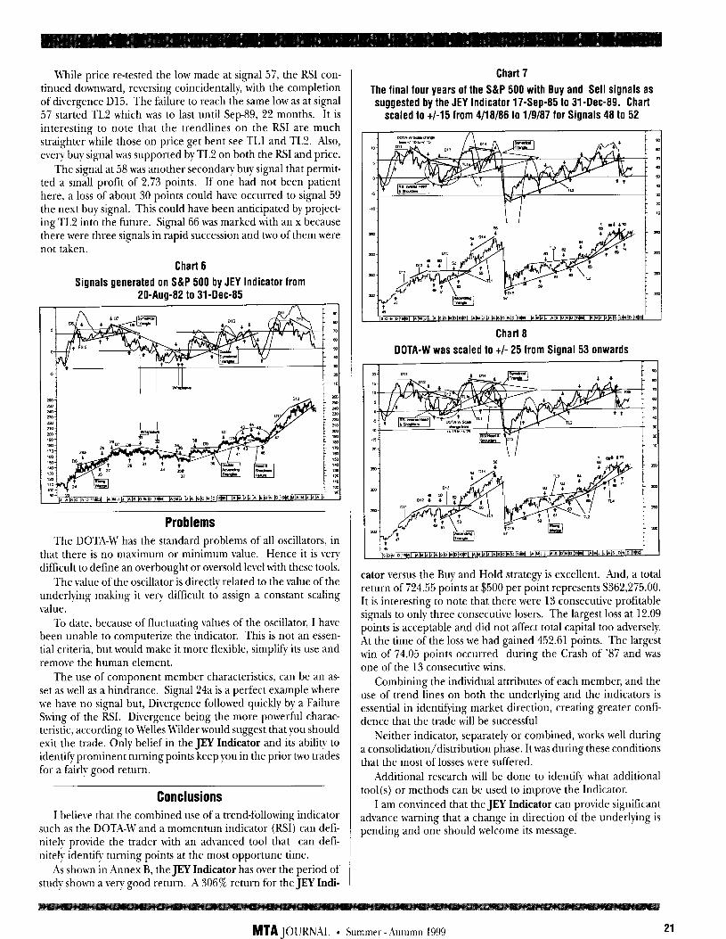
While price re-tested the low made at signal 57, the RSI continued downward, reversing coincidentally, with the completion of divergence Dl5. The failure to reach the same low as at signal 57 started TL2 which was to last until Sep-89, 22 months. It is interesting to note that the trendlines on the RSI are much straighter while those on price get bent see TLl and TL2. Also, every buy signal was supported by TL2 on both the RSI and price.

The signal at 58 was another secondary buy signal that permitted a small profit of 2.73 points. If one had not been patient here, a loss of about 30 points could have occurred to signal 59 the next buy signal. This could have been anticipated by project- ing TL2 into the future. Signal 66 was marked with an x because there were three signals in rapid succession and two of them were not taken.

Chart 6 Signals generated on S&P 500 by JEY Indicator from

20-Aug-82 to 31 -Dee-85 I

Problems The DOTA-MT has the standard problems of all oscillators, in

that there is no maximum or minimum value. Hence it is very difficult to define an overbought or oversold level with these tools.

The value of the oscillator is directly related to the value of the underlying making it very difficult to assign a constant scaling value.

To date, because of fluctuating values of the oscillator, I have been unable to computerize the indicator. This is not an essential criteria, but would make it more flexible, simplify its use and remove the human element.

The use of component member characteristics, can be an as- set as well as a hindrance. Signal 24a is a perfect example where we have no signal but, Divergence followed quickly by a Failure Swing of the RX Divergence being the more powerful characteristic, according to Welles Wilder would suggest that you should exit the trade. Only belief in the JEY Indicator and its ability to identiQ.prominent turning points keep you in the prior two trades for a fan-lp good return.

Conclusions I believe that the combined use of a trend-following indicator

such as the DOTA-W and a momentum indicator (RSI) can defi- nitely provide the trader with an advanced tool that can defi- nitely identify turning points at the most opportune time.

As shown in Annex B, theJEY Indicator has over the period of study shown a very good return. A 306% return for the JEY Indi-

Chart 7 The final four years of the S&P 500 with Buy and Sell signals as suggested by the JEY Indicator 17-Sep-85 to 31-Dee-89. Chart

scaled to +/-15 from 4/18/86 to l/9/87 for Signals 48 to 52

L

cator versus the Buy and Hold strategy is excellent. And, a total return of 724.55 points at $500 per point represents $362,275.00. It is interesting to note that there were 13 consecutive profitable signals to only three consecutive losers. The largest loss at 12.09 points is acceptable and did not affect total capital too adversely. At the time of the loss we had gained 452.61 points. The largest win of 74.05 points occurred during the Crash of ‘87 and was one of the 13 consecutive wins.

Combining the individual attributes of each member, and the use of trend lines on both the underlying and the indicators is essential in identifying market direction, creating greater confidence that the trade will be successful

Neither indicator, separately or combined, works well during a consolidation/distribution phase. It was during these conditions that the most of losses were suffered.

Additional research will be done to identify what additional tool(s) or methods can be used to improve the Indicator.

I am convinced that the JEY Indicator can provide significant advance warning that a change in direction of the underlying is pending and one should welcome its message.


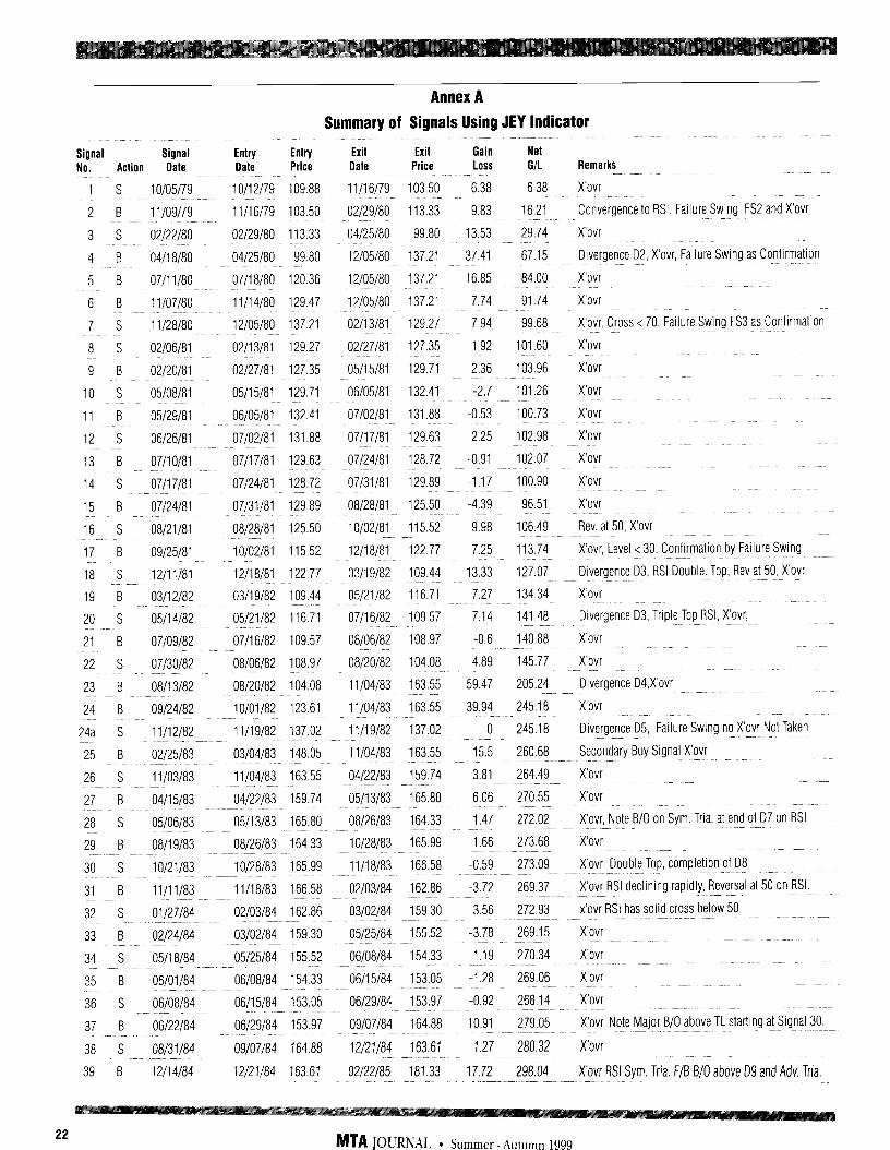
Signal Signal Entry Entry

NO. Action Date Date Price

1 S 10/05/79 10/12/79 109.88

2 B- 11/09/79 11/16/79 103:50

3 s 02/22/80 02/29/80 113.33

4 B 04/18/80 04/25/80 99.80

5 B 07/11/80 07/18/80 120.36

6 B 11/07/80 11/14/80 129.47

7 s 11/28/80 12/05/80 137.21

8 S 02/06/81 02/13/81 129.27

9 B 02/20/8; 02/27/81 127.35

10 s 05/08/81- 05/15/81 129.71

11 B 05/29/81 06/05/81 132.41

12 s 06/26/81 07/02/81 131.88

13 B 07/10/81 07/17/81 129.63

14 s 07/17/81 07124181 128.72

15 B 07124181 07/31/81 129.89

16 S 08/21/81 -08/28/81 125.50

17 B 09/25/81 10/02/81 115.52

18 S- 12/11/81 12/18/81 122.77

19 B 03/f2/82 03/19/82 109.44

20 s 05/14/82 05/21/82 116.71

21 B 07/09/82 07/16/82 109.57

22 s 07/30/82 08/06/82 108.97

23 B 08/13/82 08/20/82 104.08

24 B 09124182 10/01/82 123.61

24a S 11/12/82 11/19/82 137.02

25 B 02125183 03/04/83 148.05

26 S 11/03/83 ll/g4/83 163.55

27 B 04/15/83 04/22/83 159.74

28 -- S 05/g6/83 05/13/83 165.80

29 B 08/19/83 08/26/83 164.33

30 s 10/21/83 10/28/83 165.99

31 B 11/11/83 11/18/83 166.58

32 S 01127184 02/03/84 162.86

33 B 02124184 03/02/84 159.30

34 s 05/18/84 05125184 155.52 - -..- -. 35 --B 06/01/84 06/08/84 154.33

-- . -.- -

36 S 06/08/84 06/15/84 153.05

i 37 06122184 06/29/84 153.97.

38 -S 08/31/84 --09Jg7/84 164.88.

39 B 12114184 12121184 163.61

Annex A

Summary of Signals Using JEY Indicator

Exit Exit Gain Net Date Price Loss G/L Remarks

11/16/79 103.50 6.38 6.38 X'ovr

- 02/29/80 113.33 9.83 16.21 Convergence to RSI, Failure Swing FS2 and X'ovr

04/25/80 99.80 13.53 29.74 X'ovr

12/05/80 137.21 37.41 67.15 Divergence D2, X'ovr, Failure Swing as Confirmation

12/05/80 137.21 16.85 84.00 X'ovr

12/05/80 137.21 7.74 91.74 X'ovr

02/13/81 129.27 7.94 99.68 X'ovr, Cross < 70, Failure Swing FS3 as Confirmation

02/27/81 127.35 1.92 101.60 X'ovr

05/15/81 129.71 2.36 103.96 Xovr '

06/05/81 132.41 -2.7 101.26 X'ovr

07/02/81 131.88 -0.53 100.73 X'ovr

07/17/81 129.63 2.25 102.98 X'ovr

07124181 128.72 -0.91 102.07 X'ovr

07/31/81 l-29.89 -1.17 100.90 X'ovr

08128181 125.50 -4.39 96.51 X'ovr

10/02/81 115.52 9.98 106.49 Rev. at 50, X'ovr

12118181 122.77 7.25 113.74 X'ovr, Level< 30, Confirmation by Failure Swing

03/19/82 109.44 13.33 127:07 Divergence D3, RSI Double.Top, Rev at50, X'ovr

05/21/82 116.71 7.27 134.34 X'ovr

07/16/82 109.57 7.14 141.48 Divergence D3,Triple Top RSLX'ovr,

08/06/82 108.97 -0.S 140.88 Xovr -'

08/20/82 104.08 4.89 145.77 X'ovr

f1/04/83 163.55 59.47 205.24 Divergence D4,X'ovr

11/04/83 163.55 39194 245.18 X'ovr

1;/19/82 --- 137.02 -- 0 245.18 Divergence D5, Failure Swing no X'ovr Not Taken

11/04/83 163.55 15.5 260.68 Secondary Buy Signal X'ovr

04/22/83 159.74 3.81 264.49 X'ovr

05/13/83 165.80 6.06 270.55 X'ovr

- 08/26/83 164.33 1.47 272.02 X'ovr, Note B/O on Sym. Tria. atend of-D7on RSf

16599 10/28/83 1.66 273.68 X'ovr

11/18/83 166.58 -0.59 273.09 X'ovr Double Top, completion of D8

02/03/84 162.86 -13.72 269.37 X'ovr RSI declining rapidly, Reversal at50 on RSI.

03/02/84 159.30 3.56 272.93 x'ovr RSI has solid cross below50 . -. 05/25/84 155.52. -3.78 269.15 X'ovr

06/08/84 154.33 1.19 -270.34 X'ovr

06/15/84 153.05 -1.28 269.06 X'ovr

06/29/84 153.97 -0.92 268.14 ' Xovr

09/07/84 164.88 10.91 279.05 X'ovr, Note Major B/O above TLstarhng at Signal 30.

;2/21/84 -163.61 1.27 280.32 X’ovr

02/22/85 181.33 17.72 298.04 X’ovr RSI Sym. Tria. F/B B/O above D9 and Adv, Tria.

22 MTA JOUR~QL * Summer -Autumn 1999

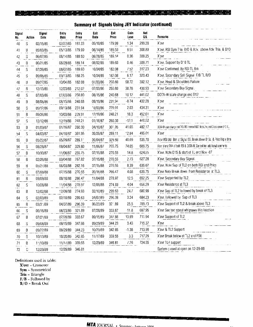
Summary of Signals Using JEY Indicator (continued)

Signal Signal Entry Entry Exit Exit Gain Net No. Action Date Date Price Date Price Loss G/L Remarks

40 s 02/15/85 02/22/85 181.33 05/10/85 179.99 1.34 299.38 X'ovr

41 B 05/03/85 05/10/85 179.99 06/14/85 189.50 9.51 308.89 X'ovr, RSI Sym Tria. B/O & Adv. above Adv. Tria. & DlO

42 S 06/07/85 06/14/85 189.50 06/28/85 189.14 0.36 309.25 X'ovr

43 B 06/21/85 06/28/85 189.14 oa/o2/85 -189.60 0.46 309.71. \'ovr,Support by DlOTL

44 s 07126185 08/02/85 189.60 io/o4/85 182.08 7.52 317.23 X'ovr Confirmed. By RSITL Brk

09/06/85 -- 45 s 09/13/85 188.25 10/04/85 182.08 6.17 323.40 X'ovr, Secondary Sell Signal F/B TL B/O

-46 -B 09/27/85 10/04/85 182.08- 07/03/86 250.80 68.72 392.12 X'ovr, Head & Shoulders Failure

-47 -B 12113/85 i2/20/85 212.02 07/03/86 250.80 38.78 430.90 X'ovr Secondary Buy Signal.

48 s 07/03/86 07/03/86 250.80 08/15/86 240.68 10.12 441.02 DOTA-Wscalechange end D12

49 B oa/oa/a6 08/15/86 -240.68 09/19/86 231.94 -a.74 432.28 X'ovr

50 s 09/12/86 09/19/86 231.94 10/03/86 229.91 2.03 434.31 X'ovr

51 B 09/26/86 10/03/86 229.91 12/19/86 248.21 la.3 452.61 X'ovr

52 S 12/12/86 12/19/86 248.21 01/16/87 260.30 -12.1 -440.52 X'ovr

53 B 01/09/87 01/16/87 260.30 04/10/87 301.95 41.65 482.17 DOTA-W scale change end 013, RSI Inverse H&S Neckline, and Cross above 013 it.

54. s 04/03/87 04/10/87 301.95 05/29/G 289.11 12.84 495.01 X'ovr

55. B 05122187 05/29/87 289.11 09/04/87 329.80 40.69 535.70 X'ovr RSI Dbl. atm atSigba153, Break above D13a, & PriceTriple Btm

56 S 08/2a/a7 09/04/87 329.80 11/06/87 255.75 74.05 609.75 X'ovr atend 014 of both RSI & DOTA-W. See text for additional comments

57 B 10/30/87 11/06/87 255.75 07/15/aa 270.55 14.8 624.55 X'ovr, Note D15 & start of TL end Nov -87

58 B 02/26/88 03/04/aa 267.82 07/15/aa 270.55 2.73 627.28 X'ovr,Secondary Buy Signal.

59 B 05/27/aa 06/03/88 262.16 07/15/aa 270.55 a.39 635.67 X'ovr, Note Sup of TL2 on both Gland Price

60 S 07/oa/aa 07/15/aa 270.55 09/16/aa 266.47 4.08 639.75 X'ovr Note Break down from Resistance atTL3.

61 B 09/09/88 09/16/aa 266.47 il/o4/aa 278.97 12.5 652.25 X'ovr Supported by TL2.

62 S 10/2a/as ii/o4/88 278.97 i2/09/aa 274.93 4.04 656.29 X'ovr Resistance atTL3

63 B 12/02/88 i2/09/aa 274.93 02/10/89 299.63 24.7 680.99 X'ovr Sup ofTL2 followed by break ofTL3

64 S 02/03/89 02/10/89 299.63 04/07/89 296.39 3.24 684.23 X'ovr, followed by Sup ofTL3

65 B 03/31/89 04/07/89 296.39 06/23/89 321.89 25.5 709.73 X'ovr SupportofTL2 & breakabove TL3 ~~~~ 06/2$39 66 s 06/16/89 321.89 i7/28/89 333.67 -11.8 697.95 X'ovr See text aboutwhipsawsthis location

67 B 07/21/89 07/28/89 333.67 09/15/89 347.66 13.99 711.94 X'ovr SupportofTL2

68 -. -- s 09/08/89 09/15/89 347.66 09/29/89 344.23 3.43 715.37 X'ovr _~ _._____-. ~.------~~..~ ---- _- - 69 B 09/22/89 09/29/89 344.23 io/20/89 342.85 -1.38 713.99 X'ovr &TL2 Support

70 s 10/13/89 10/20/89 342.85 il/l7/89 339.55 3.3 717.29 X'ovr Break below ofTL2 and FS6

71 B 1 i/lo/a9 ll/i7/89 339.55 12/29/89 346.81 7.26 724.55 X'ovrTL4 support

72 C i2/29/89 12/29/89 346.81 System closed at open on 12-29-89

Definitions used in table: X’ovr = Crossover Sym = Symmetrical Tria = Triangle F/B = Followed by B/O = Break Out

MTAJoII’~~ * Summer-Autumn 1999 39

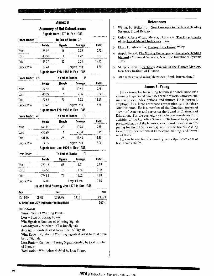
Annex B

Summary of Net Gains/losses Signals from 1979 to Feb-1983

From Trade: 1 To End of Trade: 22

Points Signals Average Ratio

Wins 156.07 16 9.75 0.73

Loss -10.30 6 -1.72 0.27

Total 145.77 22 6.63 15.15

Largest Win 37.41 Largest Loss 4.39

Signals from Feb-1983 to Feb-1986

From Trade: 23 To End of Trade: 45 - Points Signals Average Ratio

Wins 187.92 18 10.44 0.78 ~____~~ _....~~~ ~.~ Loss -10.29 5 -2.06 0.22

Total 177.63 23 7.72 18.26


Signals from Feb-1986 to Dee-1989



Wins 435.14 22 19.78 0.85

Loss -33.99 4 -8.50 0.15

Total 401.15 26 15.43 12.80

- Largest Win 74.05 Largest Loss 12.09

Signals from Jan-1979 to Dec.1989



Wins 779.13 56 13.91 0.79

Loss -54.58 15 -3.64 0.18

Total 724.55 71 10.02 14.28


Buy and Hold Strategy Jan-1979 to Dee-1989 __~

BUY Sell Net

1 O/l 2179 109.88 12129189 346.81 236.93

% Gain/Loss JEY Indicator Vs Buy/Hold 306%

Definitions:

Wii = Sum of Winning Points Loss = Sum of Losing Points Win Signals = Number of Winning Signals Loss Signals = Number of Losing Signals Average = Points divided by number of Signals Wii Ratio = Number of Winning Signals divided by total number of Signals. Loss Ratio = Number of Losing Signals divided by total number of Signals. Total ratio = Win Points divided by Loss Points.

References 1. Wilder, H. Welles, Jr., 7

Systems, Trend Research

2. Colby, Robert W. and Meyers, Thomas A., The FmcvcloDedia of Technical Market Indicators, Irwin

3. Elder, Dr. Alexander, Trading for a Living, Wiley

4. Appel, Gerald, The Movina Convereence Divexence Trading Method (Advanced Version), Scientific Investment Systems 1985

5. Murphy, John J., Technical Analvsis of the Futures Markets, New York Institute of Finance

6. All charts created using Metastock (Equis International)

James E. Young James Young has been using Technical Analysis since 1987

in timing his personal purchases or sale ofvarious investments such as stocks, index options, and futures. He is currently employed by a large aerospace corporation as a Database Administrator. He is a member of the Canadian Society of Technical Analysts and serves on the Board as Chairman of Education. For the past eight years he has coordinated the activities of the Canadian School of Technical Analysts and presented many of the lectures, which assist members in preparing for their CMT exam(s), and private traders wishing to improve their technical knowledge, trading, and investment skills.

He can be reached via e-mail: [email protected] or fax: 905/450-6102.


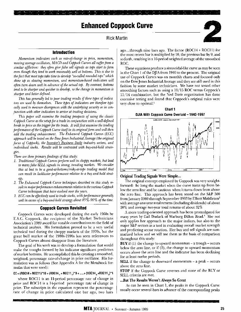
Enhanced Coppock Curve

Rick Martin

Introduction Momentum indicators such as rate-of-change in price, momentum,

moving average oscillators, MACD and Co,irpock Curves all sufferfrom a similar afJ2iction: they ojen give false sell signals as to@ start to form even though they tend to work reasonably well at bottoms. This is due to the fact that most tops take time to develop “socalled rounded tops” which show up as slowing momentum, and momentum-based indicators will often turn down well in advance of the actual top. By contrast, bottoms tend to be sharper and quicker to develop, so the change in momentum is sharper and better defined.

This has generally led to poor trading results if these types of indicators are used by themselves. These types of indicators are therefore typi- tally used to measure divergences with the underlying security or in con-

junction with other indicators to arrive at trading decisions.

This paper will examine the trading prospects of using the classic Coppock Curve as the setup for a trade in conjunction with a well-debned break in price as the trigprfor the trade. It willfirst examine the trading performance of the Coppock Curve itselfin its originalform and will then add the trading enhancement. The Enhanced Co#ock Curves (ECC) approach will be tested on the Dow Jones Industrial Average (the original focus of Coppock), the Investor’s Business Daily industry sectors, and individual stocks. Results will be contrasted with buy-and-hold strategies.

There are three primary findings of this study: 1. Traditional Coppock Curves perform well in choppy markets, but lead

to many false SELL signals in strong, trending markets. We consider this at best to be a good-at-bottoms/risky-at-tops trading model that can result in lackluster performance relative to a buy-and-hold strategy.

2. The Enhanced Coppock Curve techniques described in this stud?) result in majo-rperfmance enhancements relative to the various C@ock Curve techniques that have evolved over the gears.

3. ECC can be effectively used to trade stocks, with performance generally well in excess of a buy-and-hold strategy about 85 %-90 % of the time.

Coppock Curves Revisited Coppock Curves were developed during the early 1960s by

E.S.C. Coppock, the recipient of the Market Technicians Association’s 1989 award for notable contributions to the field of technical analysis. His formulation proved to be a very useful technical tool during the choppy markets of the 1970s but the great bull market of the 198Os-1990s has seen references to Coppock Curves almost disappear from the literature.

The goal of his work was to develop a formulation that would make the troughs formed by his indicator significant predictors of market bottoms. He accomplished this by creating a smoothed, weighted, percentage rate-of-change in price oscillator. His formulation was as follows (See Appendix A for the MetaStock for- mulas that were used) :

CC =(ROC14tROC11)'1Ot(ROC14.,tROCll~,)*9t....t(ROC14,tROC11,)*1

where ROCll is an ll-period percentage rate of change in price and ROC14 is a 14period percentage rate of change in price. The subscripts in the equation represent the percentage rate of change in price calculated one bar ago, two bars

ago....through nine bars ago. The factor (ROC14 t ROCll) for the most recent bar is multiplied by 10, the previous bar by 9, and so forth, resulting in a lo-period weighted average of the smoothed ROC.

These equations produce a sinusoidal-like curve as may be seen in the Chart 1 of the DJIA from 1940 to the present. The original use of Coppock Curves was on monthly charts and focused only on the Dow Jones Industrial Average and they are still used in this fashion by some market technicians. We have not tested other smoothing factors such as using a lo/15 ROC versus Coppock’s 11/14 combination, but the Ned Davis organization has done extensive testing and found that Coppock’s original rules were very close to optimal.’

Chart1

DJlAWith Coppock Curve Overlaid -1940-1997 LoIKi MW. cappoa Ymldrmrm Ml1 1 T

c

i 1910 IBY2 IEm 1970 IS80 11990

Original Trading Signals Were Simple... The original concept employed by Coppock was very straight-

forward: be long the market when the curve turns up from below the zero line and be cautious when it turns down from above the zero line. This approach has been tested on the S&P 500 from January 1960 through September 1993 by Elliott Middleton’ with average one-year total returns (including dividends) of about 20% and average two-year total returns of about 32%

A more trading-oriented approach has been promulgated for many years by Gail Dudack of Warburg Dillon Read.’ She not only applies her approach to the major indices, but also to the major S&P sectors as a tool in evaluating overall market strength and predicting sector rotation. Her buy and sell signals are sum- marized below and we will use them as the basis of comparison throughout this study: BUY if (1) the change to upward momentum - a trough - occurs below the zero line, or if (2), the change to upward momentum occurs above the zero line and the indicator has been declining for at least twelve periods. SELL if the change to downward momentum - a peak - occurs above the zero line. STOP if the Coppock Curve reverses and none of the BUY or SELL criteria are met. . ..But The Results Weren’t Always So Great

As can be seen in Chart 1, the peaks in the Coppock Curve usually occur several bars in advance of the corresponding peaks


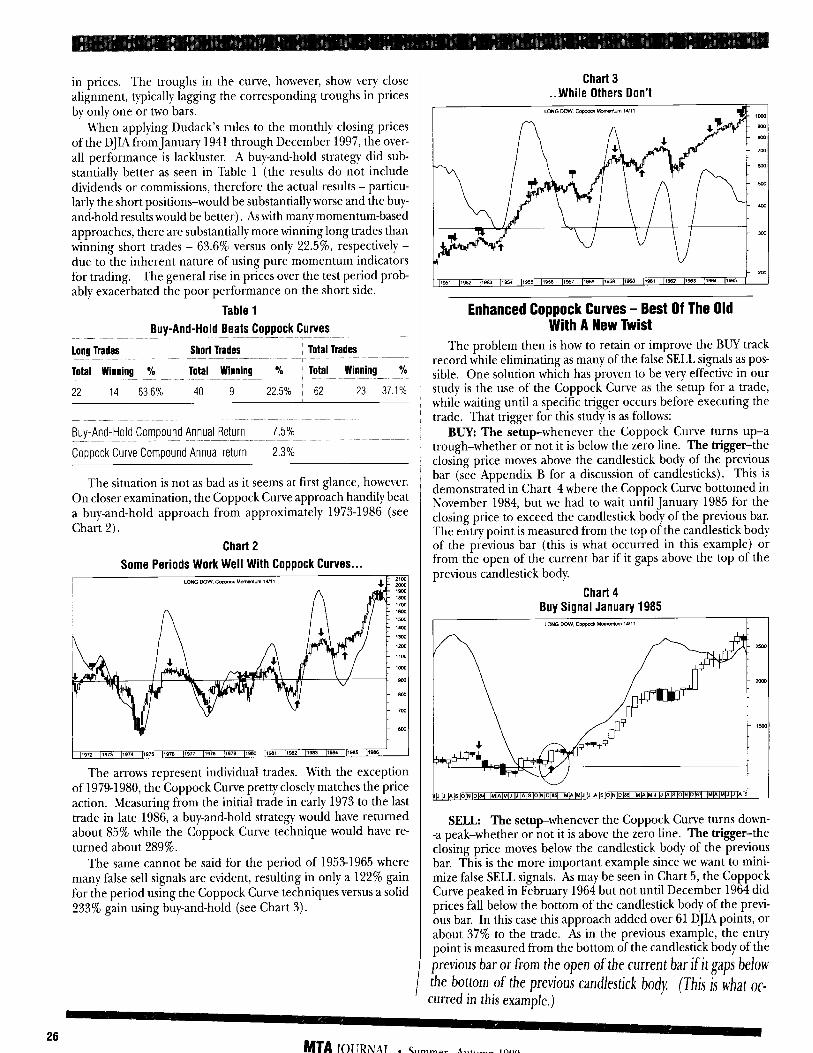
in prices. The troughs in the curve, however, show very close alignment, typically lagging the corresponding troughs in prices by only one or two bars.

When applying Dudack’s rules to the monthly closing prices of the DJIA from January 1941 through December 1997, the overall performance is lackluster. A buy-and-hold strategy did substantially better as seen in Table 1 (the results do not include dividends or commissions, therefore the actual results - particularly the short positions-would be substantially worse and the buy- and-hold results would be better). AZ with many momentum-based approaches, there are substantially more winning long trades than winning short trades - 63.6% versus only 22.5%, respectively - due to the inherent nature of using pure momentum indicators for trading. The general rise in prices over the test period prob ably exacerbated the poor performance on the short side.

Lana Trades

Table 1

Buy-And-Hold Beats Coppock Curves

Short Trades Total Trades

Total Winning % Total Winning % Total Winning % ___. ~~ _~._ _ .~_ ~~ .-... ..~~

22 14 63.6% 40 9 22.5% 62 23 37.1%

Buy-And-Hold Compound Annual Return 7.5%

Coopock Curve Compound Annual return 2.3%

The situation is not as bad as it seems at first glance, however. On closer examination, the Coppock Curve approach handily beat a buy-and-hold approach from approximately 1973-1986 (see Chart 2).

Chart 2

Some Periods Work Well With Coppock Curves...

The arrows represent individual trades. With the exception of 1979-1980, the Coppock Curve pretty closely matches the price action. Measuring from the initial trade in early 1973 to the last trade in late 1986, a buy-and-hold strategy would have returned about 85% while the Coppock Curve technique would have returned about 289%.

The same cannot be said for the period of 1953-1965 where many false sell signals are evident, resulting in only a 122% gain for the period using the Coppock Curve techniques versus a solid 233% gain using buy-and-hold (see Chart 3).

Chart 3 ..While Others Don’t

Enhanced Coppock Curves - Best Of The Old With A New Twist

The problem then is how to retain or improve the BUY track record while eliminating as many of the false SELL signals as possible. One solution which has proven to be very effective in our study is the use of the Coppock Curve as the setup for a trade, while waiting until a specific trigger occurs before executing the trade. That trigger for this study is as follows:

BW: The setup-whenever the Coppock Curve turns up-a trough-whether or not it is below the zero line. The trigger-the closing price moves above the candlestick body of the previous bar (see Appendix B for a discussion of candlesticks). This is demonstrated in Chart 4 where the Coppock Curve bottomed in November 1984, but we had to wait until January 1985 for the closing price to exceed the candlestick body of the previous bar. The entry point is measured from the top of the candlestick body of the previous bar (this is what occurred in this example) or from the open of the current bar if it gaps above the top of the prebious candlestick body.

Chart 4 Buy Signal January 1985 LONG Dow. cwwh -m 1431 t

SELL: The setup-whenever the Coppock Curve turns down- -a peak-whether or not it is above the zero line. The trigger-the closing price moves below the candlestick body of the previous bar. This is the more important example since we want to minimize false SELL signals. As may be seen in Chart 5, the Coppock Curve peaked in February 1964 but not until December 1964 did prices fall below the bottom of the candlestick body of the previous bar. In this case this approach added over 61 DJIA points, or about 37% to the trade. As in the previous example, the entry point is measured from the bottom of the candlestick body of the

previous bar or from the open of the wren t bar if it gaps below the bottom of the previous candlestick body, cmrd in this example.)

(Thy ;,y what OC-

MTA JOURNAL l Summer-Autumn IWQ

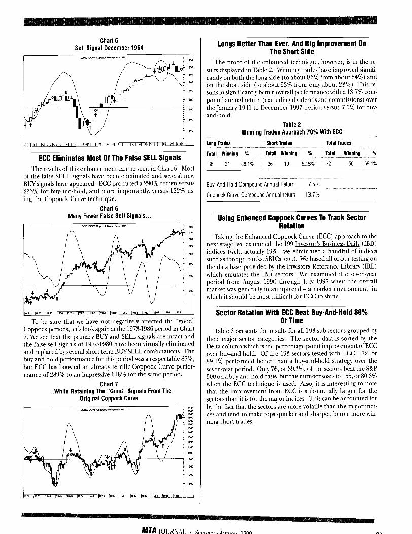
Chart 5 Sell Signal December 1964

ECC Eliminates Most Of The False SELL Signals The results of this enhancement can be seen in Chart 6. Most

of the false SELL signals have been eliminated and several new BLY signals have appeared. ECC produced a 290% return versus 233% for buy-and-hold, and more importantly, versus 122% using the Coppock Curve technique.

Chart 6 Many Fewer False Sell Signals...

61 11952 1195.3 ,19y /1955 ,I956 ,I957 /1958 1,959 11960 11961 11962 ,I963 pojl p I

To be sure that we have not negatively affected the “good” Coppock periods, let’s look again at the 19731986 period in Chart 7. We see that the primaIy BUY and SELL signals are intact and the false sell signals of 1979-1980 have been virtually eliminated and replaced by several short-term BLVSELL combinations. The buy-and-hold performance for this period was a respectable 85%, but ECC has boosted an already terrific Coppock Curve performance of 289% to an impressive 618% for the same period.

Chart 7 . ..While Retaining The “Good” Signals From The

Original Coppock Curve

longs Better Than Ever, And Big Improvement On The Short Side

The proof of the enhanced technique, however, is in the results displayed in Table 2. Winning trades have improved significantly on both the long side (to about 86% from about 64%) and on the short side (to about 53% from only about 23%). This results in significantly better overall performance with a 13.7% compound annual return (excluding dividends and commissions) over the January 1941 to December 1997 period versus 7.5% for buy- and-hold.

Table 2 Winning Trades Approach 70% With ECC

long Trades Short Trades Total Trades

Total Winning % Total Winning % Total Winning %

36 31 86.1% 36 19 52.8% 72 50 69.4%

Buy-And-Hold Compound Annual Return 7.5% . _._~ --. -- _... ~.-.-_

Coppock Curve Compound Annual return 13.7%

Using Enhanced Coppock Curves To Track Sector Rotation

Taking the Enhanced Coppock Curve (ECC) approach to the next stage, we examined the 199 Investor’s Business Daily (IBD) indices (well, actually 193 - we eliminated a handful of indices such as foreign banks, SBICs, etc.). We based all of our testing on the data base provided by the Investors Reference Library (IRL) which emulates the IBD sectors. We examined the seven-year period from August 1990 through July 1997 when the overall market was generally in an uptrend - a market environment in which it should be most difficult for ECC to shine.

Sector Rotation With ECC Beat Buy-And-Hold 89% Of Time

Table 3 presents the results for all 193 subsectors grouped by their major sector categories. The sector data is sorted by the Delta column which is the percentage point improvement of ECC over buy-and-hold. Of the 193 sectors tested with ECC, 172, or 89.1% performed better than a buy-and-hold strategy over the seven-year period. Only 76, or 39.3%, of the sectors beat the S&P 500 on a buy-and-hold basis, but this number soars to 155, or 80.3% when the ECC technique is used. Also, it is interesting to note that the improvement from ECC is substantially larger for the sectors than it is for the major indices. This can be accounted for by the fact that the sectors are more volatile than the major indices and tend to make tops quicker and sharper, hence more winning short trades.

MTAJOLXAN * Summer -Autumn 1999 27

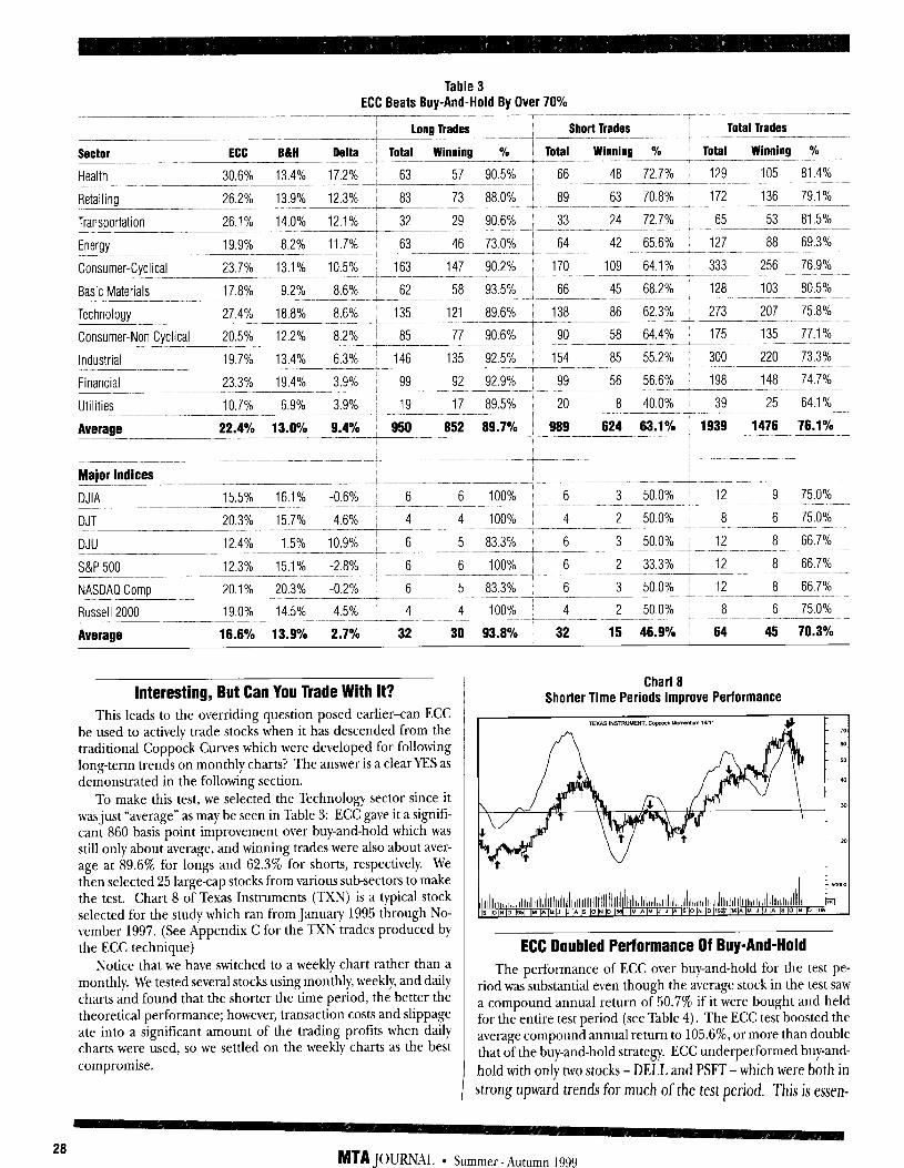
Table 3 ECC Beats Buy-And-Hold By Over 70%

long Tradw Short Trades I Total Trades

Sector ECC B&H Delta Total Winning % Total Winning % Total Winning % - Health 30.6% 13.4% 17.2% : 63 57 90.5% 66 48 72.7% 129 105 81.4%

- ~~~__~_~ -------~~~-----~~ .-.--- ~-.- Retailing 26.2% 13.9%

-

12.3% 83 73 88.0% -.2!!~ 63 70.8% 172 136 79.1% ~-~-~------ ~.~~ -- _-____

Transportation 26.1% 14.0% 12.1% I 32 -m__33 ~~-__7~1~_65~.~~~5381.~!o_ - 2g 90.6% ______ - ____-----~--~ Energy 19.9% 8.2% 11.7% 63 46 73.0% 64 42 65.6% 127 88 69.3%

Consumer-Cyclical 23.7% 13.1% 10.5% 163 147 90.2% 170 109 64.1% 333 256 76.9% - Basic Materials 17.8% 9.2% 8.6% : 62 58 93.5% 66 45 68.2% 128 103- 80.5% ~~~~ ..- ~.~ ___.. ~_~~~~~ _...._. ~~~~~~.~~~ _-.... ~~~~~ _. . ..~~~~~~~-~--.--..-.~~~.~~.. ~~. Technology 27.4% 18.8% 8.6% 135 121 89.6% 138 86 62.3% 273 207 75.8%

Consumer-Non Cyclical 20.5% 12.2% 8.2% I 85 77 90.6% 90 58 64.4% 175 135 77.1%

Industrial 19.7% 13.4% 6.3% 146 135 92.5% 154 iii 55.2% 300 220 73.3% _~___~~.~ ______.._ ~~-~~-.~.___~~----.--~~~-~ -.---- --G-- Financial 23.3% 19.4% 3.9% 99 92 92.9% 99 56 56.6% 198 148 74.7%

-~ A-~ Utilities 10.7% 6.9% 3.9% 19. 17 89.5% 20 8 40.0% 39 25 64.1% '

Average 22.4% 13.0% 8.4% 850 852 88.7% 889 824 63.1% : 1939 1476 76.1%

~~__.. ~~ ~~- ~~~ Major Indices

DJIA 15.5% 16.1% -0.6% 6 6 100% 6 3 50.0% 12 9 75.0%

DJT 20.3% 15.7% 4.6% 4 4 100% 4 2 50.0% 8 6 75.0%

-~- DJU 12.4% 1.5% 10.9% 6 5 83.3%- 6 3 50.0% 12 8 66.7%

S&P500 12.3% 15.1% -2.8% 6 6 100% 6 2 33.3% ~ 12 8 66.7% ~---~--7~-------------~-..-T --~.-~--~---- NASDAQComp 20.1% 20.3% -0.2% 6 5 83.3% 6 3 50.0% ~ 12 8 66.7% .~_-----

~-

_~--.--~~-.~.--.~-~ Russell2000 19.0% 14.5% 4.5% 4 4 100% 4 2 50.0% 8 6 75.0%

Average 16.6% 13.9% 2.7% 32 30 93.8% 32 15 46.9% 64 45 70.3%

Interesting, But Can You Trade With It? This leads to the overriding question posed earlier-can ECC

be used to actively trade stocks when it has descended from the traditional Coppock Curves which were developed for following long-term trends on monthly charts? The answer is a clear YES as demonstrated in the following section.

To make this test, we selected the Technology sector since it was just “average” as may be seen in Table 3: ECC gave it a significant 860 basis point improvement over buy-and-hold which was still only about average, and winning trades were also about average at 89.6% for longs and 62.3% for shorts, respectively. We then selected 25 large-cap stocks from various subsectors to make the test. Chart 8 of Texas Instruments (TXN) is a typical stock selected for the study which ran from January 1995 through No- vember 1997. (See Appendix C for the TXN trades produced by the ECC technique)

Notice that we have switched to a weekly chart rather than a monthly. We tested several stocks using monthly, weekly, and daily charts and found that the shorter the time period, the better the theoretical performance; however, transaction costs and slippage ate into a significant amount of the trading profits when daily charts were used, so we settled on the weekly charts as the best compromise.


Chart8 Shorter Time Periods improve Performance

ECC Doubled Performance Of Buy-And-Hold The performance of ECC over buy-and-hold for the test pe-

riod was substantial even though the average stock in the test saw a compound annual return of 50.7% if it were bought and held for the entire test period (see Table 4). The ECC test boosted the average compound annual return to 105.6%, or more than double that of the buy-and-hold strategy. ECC underperformed buy-and- hold with only two stocks - DELL and PSFT - which were both in strong upward trends for much of the test period. This is essen-

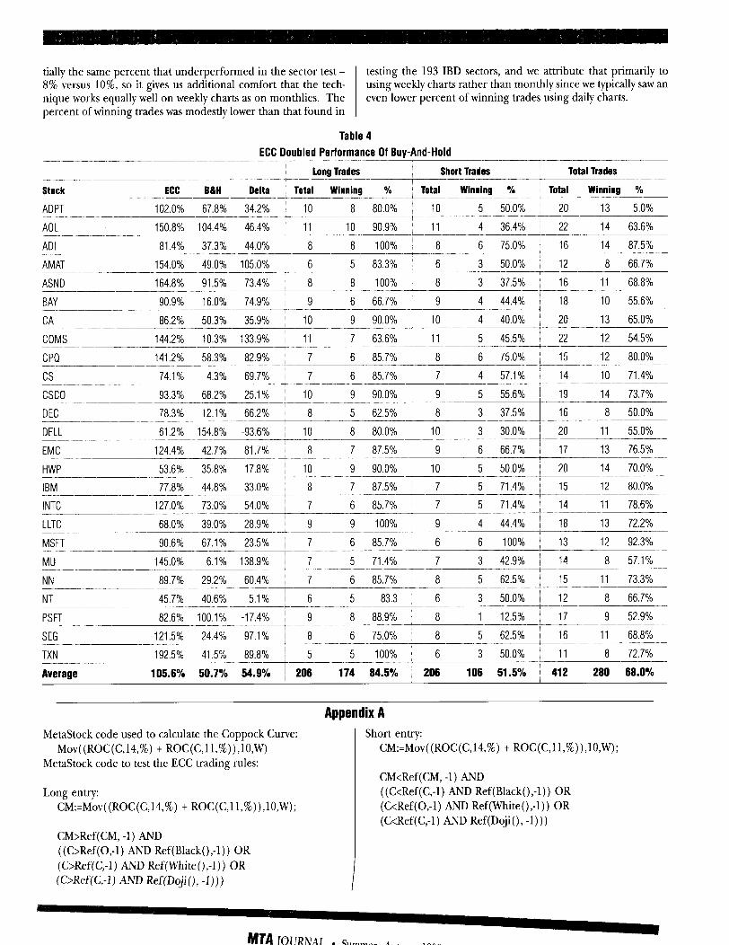
tially the same percent that underperformed in the sector test - 8% versus lo%, so it gives us additional comfort that the technique works equally well on weekly charts as on monthlies. The percent of winning trades was modestly lower than that found in

testing the 193 IBD sectors, and we attribute that primarily to using weekly charts rather than monthly since we typically saw an even lower percent of winning trades using daily charts.

Table 4

ECC Doubled Performance Of Buy-And-Hold

Lonu Trades Short Trades Total Trades

Stock ECC B&H Delta Total Winning % ! Total Winning % Total Winning %

ADPT 102.0% 67.8% 34.2% 10 8 80.0% i 10 5 50.0% 20 13 5.0%

AOL 150.8% 104.4% 46.4% 11 10 90.9% j 11 4 36.4% 22 14 63.6%

ADI 81.4% 37.3% 44.0% 8 8 100% j 8 6 75.0% 16 14 87.5%

AMAT 154.0% 49.0% 105.0% 6 5 83.3% j 6 3 50.0% i 12 8 66.7%

ASND 164.8% 91.5% 73.4% 8 8 100% j 8 3 37.5% I 16 11 68.8%

BAY 90.9% 16.0% 74.9% 9 6 66.7% / 9 4 44.4% I 18 10 55.6%

CA 86.2% 50.3% 35.9% 10 9 90.0% 10 4 40.0% j 20 13 65.0% -- COMS 144.2% 10.3% 133.9% 11 7 63.6% 11 5 45.5% I 22 12 54.5%

CPQ

cs

141.2% 58.3% 82.9% 7

74.1% 4.3% 69.7% 7

csco 93.3% 68.2% 25.1% 10 9 90.0% i 9 5 55.6% I 19 14 73.7% - .- DEC 78.3% 12.1% 66.2% 8 5 62.5% ~ 8 3 37.5% / 16 8 50.0%

- DELL 61.2% 154.8% -93.6% 10 8 80.0% 10 3 30.0% ~ 20 11 55.0%

EMC 124.4% 42.7% 81.7% 8 7 87.5% 1 9 6 66.7% ~ 17 13 76.5%

HWP 53.6% 35.8% 17.8% 10 9 90.0% : 10 5 50.0% ~ 20 14 70.0% - IBM 77.8% 44.8% 33.0% 8 7 87.5% I 7 5 71.4% 15 12 80.0%

INTC 127.0% 73.0% 54.0% 7 6 85.7% / -7 5 71.4% 14 11 78.6%

: LLTC 68.0% 39.0% 28.9% 9 9 100% 9 4 44.4% 18 13 72.2% q---- ---. MSFT 90.6% 67.1% 23.5% 7 6 85.7% ' 6 6 100% 13 12 92.3%

MU 145.0% 6.1% 138.9% 7 5 71.4% : 7 3 42.9% 14 8 57.1% c~-------------------.~.~+ ---- ~ NN 89.7% 29.2% 60.4% 7 6 85.7% : 8 5 62.5% 15 11 73.3%

NT 45.7% 40.6% 5.1% 6 5 83.3 i 6 3 50.0% 12 8 66.7%

PSFT 82.6% 100.1% -17.4% 9 8 88.9% i 8 1 12.5% 17 9 52.9%

SEG 121.5% 24.4% 97.1% 8 6- 75.0% 1 8 5 62.5% 16 11 68.8%

TXN 192.5% 41.5% 89.8% -'- 5 5 100%-j 6 3 50.0% 11 8 72.7%

Averare 105.6% 50>% 54.9% ~ 206 174 84.5% i 206 106 51.5% 412 280 68.0%

MetaStock code used to calculate the Coppock Curve: Mov((ROC(C,14,%) t ROC(C,ll,%)),lO,W)

MetaStock code to test the ECC trading rules:

Long entry: CM:=Mov((ROC(C,14,%) t ROC(C,ll,%)),I9,W);

CM>Ref(CM, -1) AND ((C>Ref(O,-1) AND Ref(Black(),-1)) OR (C>Ref(C,-1) AND Ref(White(),-I)) OR (C>Ref(C,-1) A..D Ref(Doji(), -I)))

Appendix A

Short entry: CM:=Mov((ROC(C,14,%) t ROC(C,ll,%)),lO,W);

CM<Ref(CM, -1) AND ((C<Ref(C,-1) AND Ref(Black(),-1)) OR (C<Ref(O,-1) AND Ref(White(),-1)) OR (CtRef(C,-1) AND Ref(Doji(), -1)))

MTA JOC’RNAL * Summer -Autumn 1999

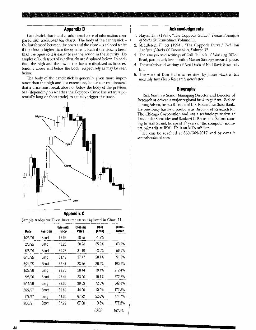
Appendix B Acknowledgments Candlestick charts add an additional piece of information com-

pared with traditional bar charts. The body of the candlestick - the bar formed between the open and the close -is colored white if the close is higher than the open and black if the close is lower than the open so it is easier to see the action in the security. Ex- amples of both types of candlesticks are displayed below. In addition, the high and the low of the bar are displayed as lines extending above and below the body respectively as may be seen below.

1. Hayes, Tim (1993), “The Coppock Guide,” Technical Analysis of Stocks & Commodities, Volume 11.

2. Middleton, Elliott (1994), “The Coppock Curve,” Technical Anal@ of Stoclzs & Commodities, Volume 12.

3. The analysis and writings of Gail Dudack of Warburg Dillon Read, particularly her monthly ,Market Strategy research piece.

4. The analysis and writings of Ned Davis of Ned Davis Research, Inc.

The body of the candlestick is generally given more importance than the high and low extensions, hence our requirement that a price must break above or below the body of the previous bar (depending on whether the Coppock Curve has set up a potentially long or short trade) to actually trigger the trade.

5. The work of Don Hahn as revisited by James Stack in his monthly InvesTech Research newsletter.

Biography Rick Martin is Senior Managing Director and Director of

Research at Advest, a major regional brokerage firm. Before joining Advest, he was Director of U.S. Research at Swiss Bank. He previously has held positions as Director of Research for The Chicago Corporation and was a technology analyst at Prudential Securities and Sanford C. Bernstein. Before com- ing to Wall Street, he spent 17 years in the computer industry, primarily at IBM. He is an MTA affiliate.

Appendix C Sample trades for Texas Instruments as displayed in Chart 11.

Gate Opening Closing Gain Cumu-

Position Price Price (Loss) lative

l/23/95 Short 18.03 18.25 -1.2%

216195 Long 18.25 30.28 65.9% 63.9%

-616195

______-______

Short 30.28 31.19 -3.0% 59.0%

6/l 5195 Long 31.19 37.47 20.1% 91.0% .---- ~~--.______ ________~

8/21195 Short 37.47 23.75 36.6% 160.9%

l/22/96

5/6/96

Long

Short

23.75 28.44 19.7% 212.4%

28.44 23.00 19.1% 272.2%

9/l l/96

-2i27/97

Long

Short

23.00 39.69 72.6% 542.3%

39.69 44.00 -10.9% 472.5%

- 717197

g/30/97

Long

Short

44.00 67.22 52.8% 774.7% ___

67.22 67.00 0.3% 777.5%

CAGR 192.5%

He can be reached at 860/509-2017 and by e-mail: [email protected]

MTA JOURNAL l Summer -Autumn IQQQ

The Anchor Breakout

A Technical Pattern Derivative

Stephen W. Cox, CMT

Introduction-A Basic Concept of Chart Pattern The topic of the following paper is a way of thinking, specifically, the

idea that chart patterns are PrOperly seen as manifestations of a single general concept.

My intent is to argue, first, that the technician’s “cookbook” of basic chart patterns can be generalized and, second, that such a generalization naturally leads full circle to a possibly unlimited number of particular chart patterns in addition to those in the current vocabulary of technical analysis. In support of this argument I will describe a particular pattern that is, to my knowledge, an original infuence-and the word “infer- encez is deliberate. I will show that this pattern, which I will call the “Anchor Breakout” pattern, is often a signal of important support and resistance points, which is what price targets are.

This paper does not imply that the Anchor Breakout pattern is infallible or even is the most reliable chart pattern. Its point is that the Anchor Breakout pattern has been derived by inference from a general concept, an important point given that the concepts of technical analysis are em@- tally derived and therefore under suspicion of being arbitrary or subjec- tive. Its suggestion is that technical analysis is ultimately a logical en- deavor

The basis of technical market analysis is pattern, a definable or mi- nutely describable sequence of events in any one of innumerable forms of market action. Each pattern has a beginning and an ending that carries definite implications for subsequent market action. A given pattern may be sophisticated and extended. For example, the market begins to sell off at a date that is the square root of the twenty-ninth Fibonacci number times 29.5 days after the date of a preuious prominent selloff (Carolan, 1992, 41). The sequence is the previous market high, another high afer the passage of a definable time, then the conclusion, based on historical observation, that the market may be due to change direction from up to down because that definable time has passed. The pattern in this case is a correlation between market movement and time.

A pattern rather may be brief and uncomplicated, the breaking of a support linefor example. In that case the sequence of events is thepredeter- mination of a support/resistance line, the breakdown of the market below that line, then finally the conclusion, again based on historical obserua- tion, that the market has weakened. A similar example would be the crossing of a market above its moving average. In this case the pattern is a change in the market’s relationship to a given support/resistance line.

Pattern as described in this paper is arguably a pattern of the pure4 geometric type as in the second, uncomplicated example. This type of

pattern is what market technicians commonly mean by the phrase “chart pattern. ” This paper assumes that the reader is familiar with the basic chart patterns as described in the literature of technical analysis. There- fore, no attempt is made to describe these common patterns beyond citation of that literature.

Chart Pattern, A Reduction It can be shown that the dozen or so chart patterns described

in the literature and their variants can be reduced to a mere handful of rVorking patterns. Jloreorrc it can be shown that common& accepted chart pattern ana&is in most cases uses a single

I

methodology. First, the market traces out a geometric shape that in most cases is symmetrical about a straight line. Second, the market breaks out of the shape. Third, the height of the shape is projected vertically in the direction of the break, up or down, to derive a minimum price target.

It is remarkable that the relatively brief number of chart patterns in the technical analysis literature can be made even more compact by generalization.

It turns out that most of the reversal patterns, that is the patterns that are formed at the end of a market trend, are in fact varieties of the head and shoulders formation (Murphy, 1986, Pp 107, 118, 121).

Authorities note that the rare diamond formation can in fact involve a broadening formation or a head and shoulders formation (Edwards and Magee, 1966, 151). A diamond, which is typically a broadening formation joined with a symmetrical triangle, tends to be symmetrical about the lines connecting its diagonally opposite apexes (Murphy, 1986, 153). When the market breaks out of a diamond formation, the largest vertical dimension of the diamond is projected vertically (Edwards and Magee, 1966, 154).

Flags and pennants, which typically occur “at half mast,” that is, at the halfway point of a market move, are variants of the measured move (Murphy, 1986, 167). The pennant involves a triangu- lar consolidation formation.

The measuring technique for double and triple tops or bottoms uses the vertical height of the pattern. The double and triple top or bottom formations can be interpreted as rectangular reversal patterns (Murphy, 1986, pp 123, 165).

The measured move and the measuring gap are practically equivalent patterns. In the case of a measuring gap, a chart gap takes the place of the consolidation formation between two legs of a market move. In a bull market, for example, the market tends to move as far above the gap as it moved approaching the gap (Edwards and Magee, 1966, pp 198-202).

Evidently, therefore, there are essentially only four chart patterns that have measuring implications: the triangle, the rectangle, the head and shoulders, and the measured move. There are of course chart patterns such as the saucer and the V-formation that don’t enable the technician to make price measurements. But it’s safe to say that the triangle, the rectangle, the head and shoulders, and the measured move include most of the patterns commonly found on the charts.

The Principle of Symmetry The four essential chart patterns with measuring implications,

the triangle, the rectangle, the head and shoulders, and the measured move, share a notable characteristic, namely geometric symmetry about a straight line. This means that the pattern can be divided by one or more straight lines into two shapes, usually equal in dimension, that are related as mirror images.

A triangle is symmetrical about the strai,ght line connecting its

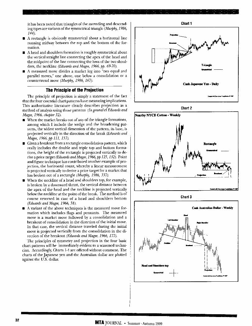
it has been noted that triangles of the ascending and descending types are variants of the symmetrical triangle (Mu$L~, 1986, 144).

q A rectangle is obviously symmetrical about a horizontal line running midway between the top and the bottom of the formation.

q A head and shoulders formation is roughly symmetrical about the vertical straight line connecting the apex of the head and the midpoint of the line connecting the lows of the two shoulders, the neckline (Edwards and Magee, 1966, pp. 69-70).

II A measured move divides a market leg into “two equal and parallel moves,” one above, one below a consolidation or a countertrend move (Murphy, 1986, 167).

The Principle of the Projection The principle of projection is simply a statement of the fact

that the four essential chart patterns have measuring implications. This authoritative literature clearly describes projection as a method of analysis using those patterns (In general cf Edwards and Magee, 1966, chapter 32).

q When the market breaks out of any of the triangle formations, among which I include the wedge and the broadening patterns, the widest vertical dimension of the pattern, its base, is projected vertically in the direction of the break (Edwards and Magee, 1966, Pp 111, 157).

II Given a breakout from a rectangle consolidation pattern, which really includes the double and triple top and bottom formations, the height of the rectangle is projected vertically to derive a price target (Edwards and Magee, 1966, pp 125,132). Point and figure technique has contributed another example of projection, the horizontal count, whereby a linear measurement is projected vertically to derive a price target for a market that has broken out of a rectangle (Murphy, 1986, 337).

q When the neckline of a head and shoulders top, for example, is broken by a downward thrust, the vertical distance between the apex of the head and the neckline is projected vertically below the neckline at the point of the break. The method is of course reversed in case of a head and shoulders bottom (Edwards and Magee, 1966, 58).

q A variant of the above techniques is the measured move formation which includes flags and pennants. The measured move is a market move followed by a consolidation and a breakout of consolidation in the direction of the initial move. In that case, the vertical distance traveled during the initial move is projected vertically from the consolidation in the direction of the breakout (Edwards and Magee, 1966, 177).

The principles of symmetry and projection in the four basic chart patterns will be immediately evident to a seasoned technician. Accordingly, Charts l-4 are offered without comment. The charts of the Japanese yen and the Australian dollar are plotted against the U.S. dollar.

Chart1

--

Cash Japanese Yen - Daily

-*Dahr-.I8

Chart2

I Nearby NYCE Cotton -Weekly

I

Chart3

Cash Awtrdhn Ddhr -Weekly


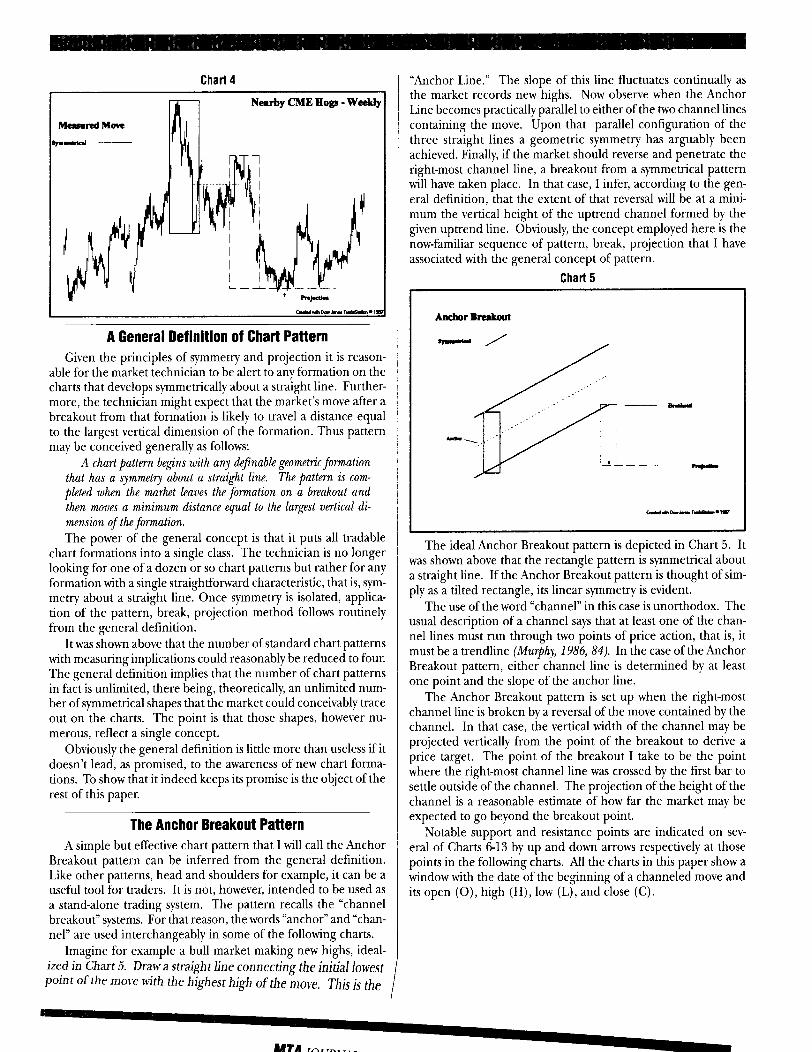
Chart4

Necrrby CME Hogs -Weekly

MwmdMove

byI.ad ___

Y

1

A General Definition of Chart Pattern Given the principles of symmetry and projection it is reason-

able for the market technician to be alert to any formation on the charts that develops symmetrically about a straight line. Further- more, the technician might expect that the market’s move after a breakout from that formation is likely to travel a distance equal to the largest vertical dimension of the formation. Thus pattern may be conceived generally as follows:

A chart pattern begins with any &@zable geometric formation that has a symmetry about a straight line. The pattern is completed when the market kaues the fmmation on a breakout and then moues a minimum distance equal to the largest vertical dimension of the fmmation.

The power of the general concept is that it puts all tradable chart formations into a single class. The technician is no longer looking for one of a dozen or so chart patterns but rather for any formation with a single straightforward characteristic, that is, symmetry about a straight line. Once symmetry is isolated, application of the pattern, break, projection method follows routinely from the general definition.

It was shown above that the number of standard chart patterns with measuring implications could reasonably be reduced to four. The general definition implies that the number of chart patterns in fact is unlimited, there being, theoretically, an unlimited number of symmetrical shapes that the market could conceivably trace out on the charts. The point is that those shapes, however numerous, reflect a single concept.

Obviously the general definition is little more than useless if it doesn’t lead, as promised, to the awareness of new chart formations. To show that it indeed keeps its promise is the object of the rest of this paper.

The Anchor Breakout Pattern A simple but effective chart pattern that I will call the Anchor

Breakout pattern can be inferred from the general definition. Like other patterns, head and shoulders for example, it can be a useful tool for traders. It is not, however, intended to be used as a stand-alone trading system. The pattern recalls the “channel breakout” systems. For that reason, the words “anchor” and “channel” are used interchangeably in some of the following charts.

Imagine for example a bull market making new highs, ideal- ized in Chart 5. Draw a straight line connecting the initial lowest

Point of the move with the highest high of the move. This js the ,

“Anchor Line.” The slope of this line fluctuates continually as the market records new highs. Now observe when the Anchor Line becomes practically parallel to either of the two channel lines containing the move. Upon that parallel configuration of the three straight lines a geometric symmetry has arguably been achieved. Finally, if the market should reverse and penetrate the right-most channel line, a breakout from a symmetrical pattern will have taken place. In that case, I infer, according to the general definition, that the extent of that reversal will be at a minimum the vertical height of the uptrend channel formed by the given uptrend line. Obviously, the concept employed here is the now-familiar sequence of pattern, break, projection that I have associated with the general concept of pattern.

Chart5

Amber Breakout

-/

The ideal Anchor Breakout pattern is depicted in Chart 5. It was shown above that the rectangle pattern is symmetrical about a straight line. If the Anchor Breakout pattern is thought of simply as a tilted rectangle, its linear symmetry is evident.

The use of the word “channel” in this case is unorthodox. The usual description of a channel says that at least one of the channel lines must run through two points of price action, that is, it must be a trendline (Murphy, 1986, 84). In the case of the Anchor Breakout pattern, either channel line is determined by at least one point and the slope of the anchor line.

The Anchor Breakout pattern is set up when the right-most channel line is broken by a reversal of the move contained by the channel. In that case, the vertical width of the channel may be projected vertically from the point of the breakout to derive a price target. The point of the breakout I take to be the point where the right-most channel line was crossed by the first bar to settle outside of the channel. The projection of the height of the channel is a reasonable estimate of how far the market may be expected to go beyond the breakout point.

Notable support and resistance points are indicated on several of Charts &13 by up and down arrows respectively at those points in the following charts. All the charts in this paper show a window with the date of the beginning of a channeled move and its open (0), high (H), low (L), and close (C).

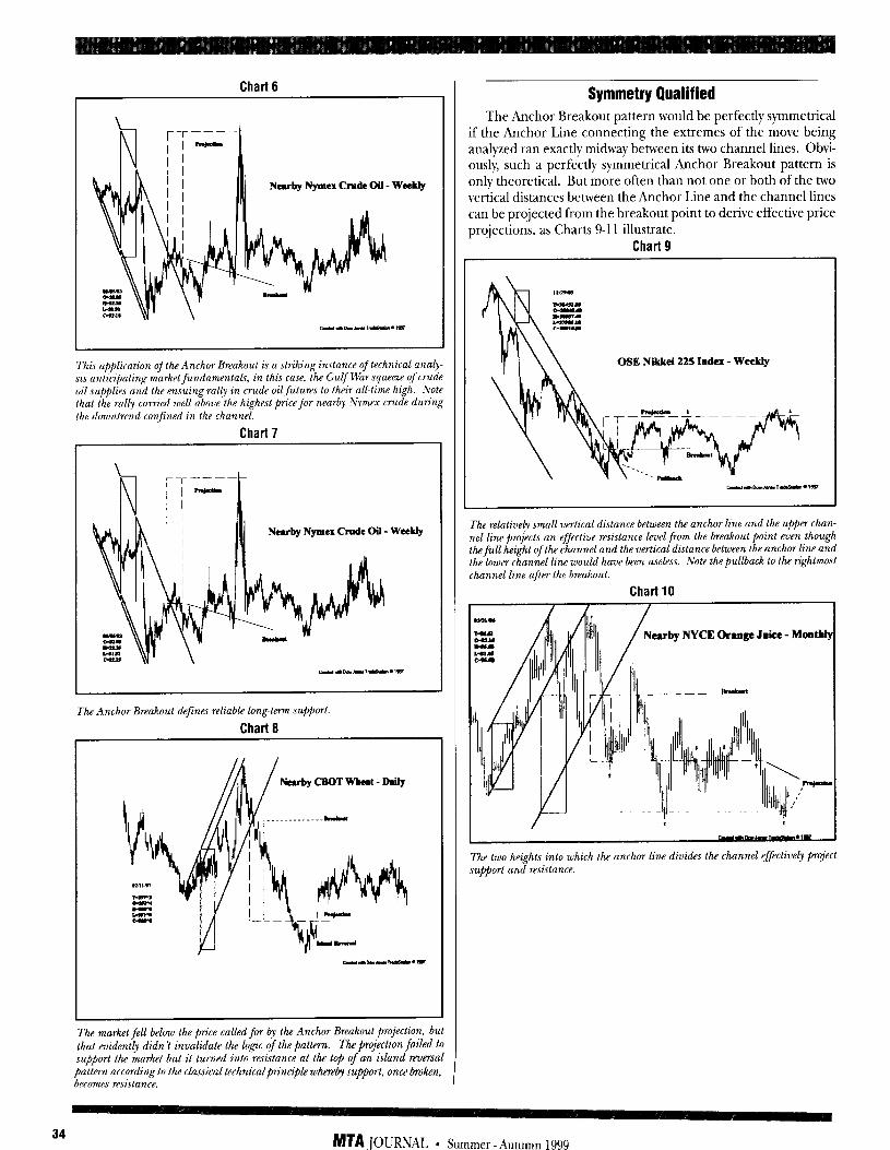
Chart6 Symmetry Qualified

r-r----- l /- I

The Anchor Breakout pattern would be perfectly symmetrical if the Anchor Line connecting the extremes of the move being analyzed ran exactly midway between its two channel lines. Obvi-

urby Nymex Crude Oil - Weekly

ously, such a perfectly symmetrical Anchor Breakout pattern is only theoretical. But more often than not one or both of the two vertical distances between the Anchor Line and the channel lines can be projected from the breakout point to derive effective price projections, as Charts 9-l 1 illustrate.

Chart9

Thic application of the Anchor Breakout is a striking instance of technical analy

sis anticibatinP market fundamentals. in this case, the Gulf War squeeze of crude

OSE Nikkei 225 Index - Weekly

m

oil supplies and the ensking rally in crude oilfutures to thd.7 all-&e high. L\Tote that the rally carried well above the highest price for nearby ?$vnex crude during the downtrend conJined in the channel.

Chart7

\n r-r----- I

I II The relative4 small vertical distance between the anchor line and the upper chan-

nel line projects an effective resistance level from the breakout point even though thefull height of the channel and the vertical distance between the anchor line and the lower channel line would have been useless. Note the pullback to the rightmost

channel line afttm the breakout.

Chart10

earby Nymex Crude Oil - Weekly

earby NYCE Orange Juice - Moatlab

The Anchor Breakout defines reliable long-term support.

Chart8 I

Nearby CBOT What - Daily /I

The two heights into which the anchor line divides the channel effective4 project support and resistance.

L

The market fell below the price called for by the Anchor Breakout projection, but

that evidently didn ‘t invalidate the logic of the pattern. The @j&on faibd to support the market but it turned into resistance at the top of an island reversal pattern according to the classical technicalfi’nciple when$ suflort, once b&en, becomes resistance.


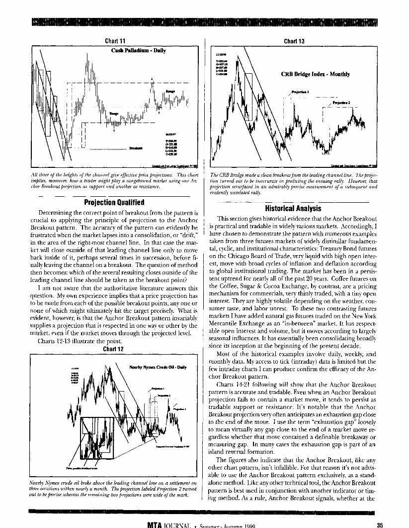
Chart11

All three of the heights of the channel give effective pn’ce projections. Thir cha

implies, moreovn, how a trader might play a rangebound market using one AI char Breakout pmjection as support and another as resistance.

Projection Qualified Determining the correct point of breakout from the pattern i

crucial to applying the principle of projection to the Ancho Breakout pattern. The accuracy of the pattern can evidently bl frustrated when the market lapses into a consolidation, or “drift, in the area of the right-most channel line. In that case the mai ket will close outside of that leading channel line only to movl back inside of it, perhaps several times in succession, before fi nally leaving the channel on a breakout. The question of methoc then becomes: which of the several resulting closes outside of the leading channel line should be taken as the breakout point?

I am not aware that the authoritative literature answers thi question. My own experience implies that a price projection ha to be made from each of the possible breakout points, any one o none of which might ultimately hit the target precisely. What i evident, however, is that the Anchor Breakout pattern invariabl supplies a projection that is respected in one way or other by the market, even if the market moves through the projected level.

Charts 12-13 illustrate the point. Chart12

I

Nearby Nymex mde oil broke above the leading channel line on a settbment o?

three occasions within nearly a month. The projection labeled Projection 2 turner out to be precise whereas the remaining two projections were wide of the mark.

Chart13

CBB Bridge Index - Monthly

The CRB Bridge made a clean breakout from the leading channel line. Theprojec- tion turned out to be inaccurate in predicting the ensuing rally. However; that projection resurfaced in an admirab<y precise measurement of a subsequent and eoident~ unrelated rally.

Historical Analysis This section gives historical evidence that the Anchor Breakout

is practical and tradable in widely various markets. Accordingly, I have chosen to demonstrate the pattern with numerous examples taken from three futures markets of widely dissimilar fundamental, cyclic, and institutional characteristics: Treasury Bond futures on the Chicago Board of Trade, very liquid with high open interest, move with broad cycles of inflation and deflation according to global institutional trading. The market has been in a persis- tent uptrend for nearly all of the past 20 years. Coffee futures on the Coffee, Sugar & Cocoa Exchange, by contrast, are a pricing mechanism for commercials, very thinly traded, with a tiny open interest. They are highly volatile depending on the weather, consumer taste, and labor unrest. To these two contrasting futures markets I have added natural gas futures traded on the New York Mercantile Exchange as an “in-between” market. It has respectable open interest and volume, but it moves according to largely seasonal influences. It has essentially been consolidating broadly since its inception at the beginning of the present decade.

Most of the historical examples involve daily, weekly, and monthly data. My access to tick (intraday) data is limited but the few intraday charts I can produce confirm the efficacy of the An- chor Breakout pattern.

Charts 1421 following will show that the Anchor Breakout pattern is accurate and tradable. Even when an Anchor Breakout projection fails to contain a market move, it tends to persist as tradable support or resistance. It’s notable that the Anchor Breakout projection very often anticipates an exhaustion gap close to the end of the move. I use the term “exhaustion gap” loosely to mean virtually any gap close to the end of a market move regardless whether that move contained a definable breakaway or measuring gap. In many cases the exhaustion gap is part of an island reversal formation.

The figures also indicate that the Anchor Breakout, like any other chart pattern, isn’t infallible. For that reason it’s not advis- able to use the Anchor Breakout pattern exclusively, as a stand- alone method. Like any other technical tool, the Anchor Breakout pattern is best used in conjunction with another indicator or timing method. As a rule, Anchor Breakout signals, whether at the

MTA JOClWAL l Summer-Autumn 1999 35

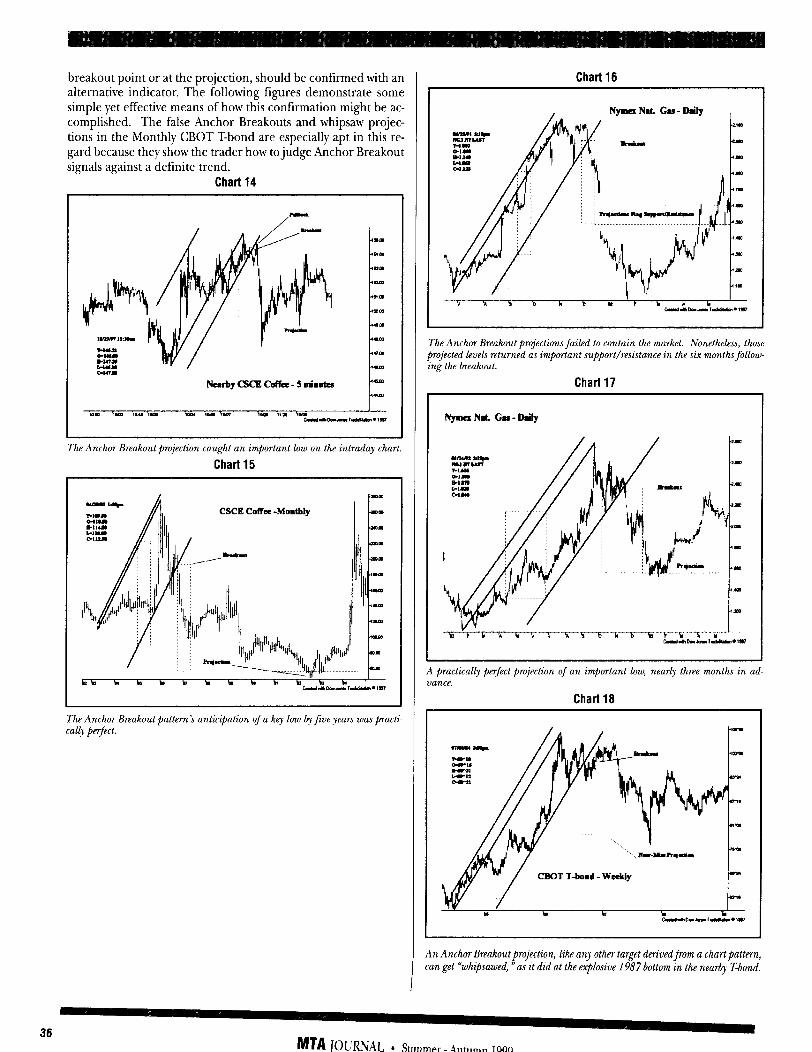
breakout point or at the projection, should be confirmed with an alternative indicator. The following figures demonstrate some simple yet effective means of how this confirmation might be accomplished. The false Anchor Breakouts and whipsaw projections in the Monthly CBOT T-bond are especially apt in this regard because they show the trader how to judge Anchor Breakout signals against a definite trend.

Chart14 I

L

ha

4-m

4-m

-

.lom

Chart15

I

CSCE Coffee -MomtIdy

Chari

The Anchor Breakout projection caught an important low on the intraday chart. I

The Anchor Breakout projections failed to contain the market. Nonetheless, those projected levels returned as impdant support/resistance in the six months follow ing the breakout.

Chart17

NymaNd Gas-Daily

A practically perfect projection of an important low, nearly three months in advance.

I ( Chart18

The Anchor Breakout pattern’s anticipation of a kq low by jive gears was practi- callj perfect.

An Anrhw Breakout projection, like any otht+r target deriurdfrom a rhartpattern, can get “whipsawed, n as it did at the explosive 1987 bottom in the nearby T-bond.

36 MTAJOLRNAL l Summer -Autumn 1999

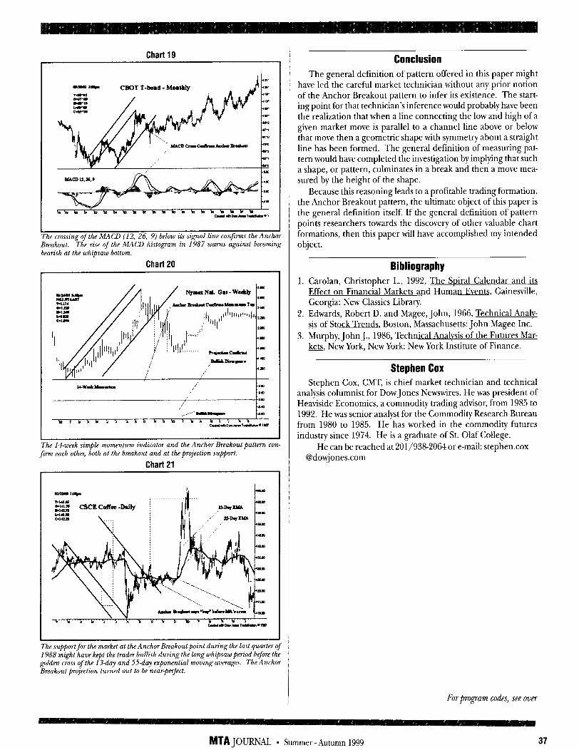
Chart19

-ac CBOT T-bond - Monthly

1 The crossing of the MAW (12, 26, 9) below its signal line confirms the Anchor

Breakout. The rise of the MAW histogram in 1987 W~TILS against becoming bearish at the whipsa; bottom,

Chart20

ke 14.week simple momentum indicator and the Anchor Breakout pattern firm each othq both at the breakout and at the projection su@ort.

Chart21

The supPortfw the market at the Anchor Breakout point dun‘ng the last quarter I988 might have kept the trader bullish during the long whipsaw period before 1

golden woss of the 13.day and 55.day exponential moving averages. The And Breakout projection turned out to be near-perfect.

Conclusion The general definition of pattern offered in this paper might

have led the careful market technician without any prior notion of the Anchor Breakout pattern to infer its existence. The starting point for that technician’s inference would probably have been the realization that when a line connecting the low and high of a given market move is parallel to a channel line above or below that move then a geometric shape with symmetry about a straight line has been formed. The general definition of measuring pattern would have completed the investigation by implying that such a shape, or pattern, culminates in a break and then a move measured by the height of the shape.

Because this reasoning leads to a profitable trading formation, the Anchor Breakout pattern, the ultimate object of this paper is the general definition itself. If the general definition of pattern points researchers towards the discovery of other valuable chart formations, then this paper will have accomplished my intended object.

Bibliography 1. Carolan, Christopher L., 1992, The Sniral Calendar and its

Effect on Financial Markets and Human Events, Gainesville, Georgia: New Classics Library.

2. Edwards, Robert D. and Magee, John, 1966, Technical Analv- sis of Stock Trends, Boston, Massachusetts: John Magee Inc.

3. Murphy, John J., 1986, Technical Analvsis of the Futures Mar- h, New York, New York: New York Institute of Finance.

Stephen Cox Stephen Cox, CMT, is chief market technician and technical

analysis columnist for Dow Jones Newswires. He was president of Heaviside Economics, a commodity trading advisor, from 1985 to 1992. He was senior analyst for the Commodity Research Bureau from 1980 to 1985. He has worked in the commodity futures industry since 1974. He is a graduate of St. Olaf College.

He can be reached at 201/938-2064 or e-mail: stephen.cox Qdowjonescom

For popam codes, see over

MTA JOURNAL l Summer-Autumn 1999 37

Appendix

Program Code The following EasyLanguageT” program has been provided to

allow analysts and traders who use or are familiar with Omega Research’s TradeStation to experiment with the Anchor Breakout pattern. The program was developed with the assistance of Fred G. Schutzman, CMT. This program is simply a descriptive tool included for the benefit of TradeStation users who want to apply the Anchor Breakout as a TradeStation Indicator. As noted previously, this is not a stand-alone trading system.

In the program, the straight line connecting the lowest and highest points of a market move is referred to code as the “anchor” line, while the channel lines of the program refer to two lines parallel to the anchor, one above it, one below, that contain the market move being analyzed.

The projection of the vertical dimension of the channel is not accomplished in the following EasyLanguage program. Rather the user can make the projection using computer drawing objects once the code is applied. I first measure the height of the channel using the rectangle in TradeStation’s library of drawing objects. Then I move a duplicate rectangle to the breakout point in order to project a price target, as seen in the figures in the previous sections. // fileName: Anchor Breakout // Written by the author and Fred G. Schutzman, CMT // Logic by the author // Program plots 1 straight line connecting two extremes (low-

to-high or high-to-low) // and 2 parallel channel lines, one below and one above the

straight line // Date last changed: December 1, 1997

Indicator Properties Style (for all 3 plots): Type = line Style = - Color = your choice Weight = lightest scalillg: Scale type = screen Axis type = linear Properties:

Max number of bars study will reference = either auto-detect or user specified of 1

check Enable Alert check box to enable alert check Update every tick check box to update with each and every

tick

Format Indicator ( applicable when you apply indicator to a chart ) Inputs: trend must be set to either tl (to draw an up trend channel) or -

1 (to draw a down trend channel) sDate (date of price bar (low or high) to begin drawing initial

straight line from) must be typed in by user Properties:

change Subgraph to one

Inputs:

trend(O), ( tl = up, -1 = down } sDate (0)) ( date of price bar (low or high) to begin draw-

ing initial straight line from } extRight(true), ( extends all 3 lines to the right if set to true ) extLeft (false) ; ( extends all 3 lines to the left if set to true ) ( the first 5 variables below match the arguments for the built-in

function TL-NEW syntax for this function is as follows: TL-New(sDate,sTime,sVal,eDate,eTime,eVal) )

Variables:

sTime (0)) { beginning or starting time of straight line }

sVal(O), ( beginning or starting ualue of straight line }

eDate (O), ( ending date of straight line (

eTime (0)) ( ending time of straight line } eVal(O), { ending value of straight line )

bBar(O), / currentBar number ofsDate }

eBar(O), / currentBar number ofeDate }

barsInStrLine (0) , ( number of price bars from the beginning to the end of the straight line }

numUsed (0)) ( counts # of array elements that have been used }

strLineValue(O), ( daily values of straight line }

maxNeg(O), ( maximum negative distance between original straight line and lowest low }

maxPos (0)) ( maximum positive distance between original straight line and highest high }

slopeOIStrLine (O);( slope of straight line ) Arrays:

barDate [500] (0) , ( stores the date of each barfrom the beginning to the end of the straight line }

barTime [500] (0), ( stores the time of each barfrom the beginning to the end of the straight line }

barLow[500] (0)) ( stores the low of each barfrom the beginning to the end of the straight line }

barHigh[500] (0)) ( stores the high of each barfrom the beginning to the end of the straight line }

barClose[500] (0); ( stores the close of each bar from the beginning to the end of the straight line )

( define or initialize first 7 variables ) if date = sDate then begin if trend = tl then begin

sTime = time; sVa1 = low; eDate = date; eTime = time; eVa1 = close;

end else if trend = -1 then begin

sTime = time; sVa1 = high;

eDate = date; eTime = time; eVa1 = close;

end; bBar = currentBar; eBar = currentBar;

end;


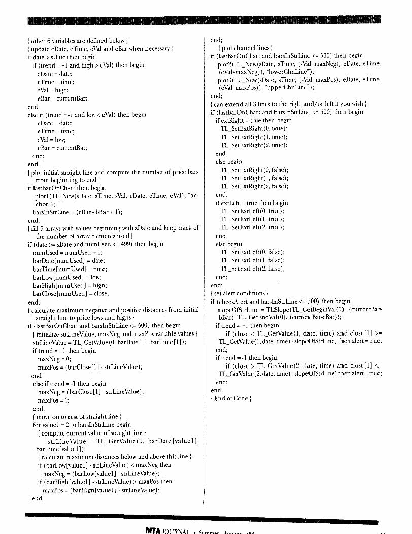
( other 6 variables are defined below ) ( update eDate, eTime, eVa1 and eBar when necessary ) if date > sDate then begin

if (trend = tl and high > eVa1) then begin eDate = date; eTime = time; eVa1 = high; eBar = currentBar;

end else if (trend = -1 and low < eVa1) then begin

eDate = date; eTime = time; eVa1 = low; eBar = currentBar;

end; end; ( plot initial straight line and compute the number of price bars

from beginning to end ) if 1astBarOnChart then begin

plot1 (TL-New(sDate, sTime, sVa1, eDate, eTime, eVal), “anchor”);

barsInStrLine = (eBar - bBar $ 1); end; ( fill 5 arrays with values beginning with sDate and keep track of

the number of array elements used } if (date >= sDate and numUsed <= 499) then begin

numUsed = numUsed -t 1; barDate [numused] = date; barTime [numused] = time; barLow [ numUsed] = low; barHigh [numused] = high; barClose [numused] = close;

end; ( calculate maximum negative and positive distances from initial

straight line to price lows and highs } if (1astBarOnChart and barsInStrLine <= 500) then begin

( initialize strlinevalue, maxNeg and maxPos variable values ] strLineValue = TL-GetValue(0, barDate[l], barTime[l]); if trend = tl then begin

maxNeg = 0; maxPos = (barClose[ l] - strlinevalue);

end else if trend = -1 then begin

maxNeg = (barClose[l] - strlinevalue); maxPos = 0;

end; { move on to rest of straight line ) for value1 = 2 to barsInStrLine begin

( compute current value of straight line ) strLineValue = TL-GetValue(0, barDate[valuel],

barTime[valuel]); ( calculate maximum distances below and above this line ) if (barLow[valuel] - strlinevalue) < maxNeg then

maxNeg = (barLow[valuel] - strlinevalue); if (barHigh[valuel] - strlinevalue) > maxPos then

maxPos = (barHigh[valuel] - StrLineVaJue); end;

end; ( plot channel lines )

if (1astBarOnChart and barsInStrLine <= 500) then begin plot2(TL_New(sDate, sTime, (sVal-tmaxNeg), eDate, eTime, (eValtmaxNeg)), “1owerChnLine”); plot3(TL_New(sDate, sTime, (sValtmaxPos), eDate, eTime, (eVal+maxPos)), “UpperChnLine”);

end; ( can extend all 3 lines to the right and/or left if you wish } if (1astBarOnChart and barsInStrLine <= 500) then begin

if extRight = true then begin TL-SetJXxtRight(0, true); TL-SetExtRight(1, true); TL-SetExtRight(2, true);

end else begin

TL-SetExtRight(0, false); TL-SetExtRight( 1, false); TL-SetExtRight(2, false);

end; if extLeft = true then begin

TL-SetExtLeft(0, true); TL-SetExtLeft(1, true); TL-SetExtLeft(2, true);

end else begin

TL-SetExtLeft(0, false); TL-SetExtLeft ( 1, false) ; TL-SetExtLeft (2, false) ;

end; end; ( set alert conditions } if (checkAlert and barsInStrLine <= 500) then begin

slopeOfStrLine = TLSlope(T/GetBeginVal(O), (currentBar- bBar) , TL-GetEndVal(0) , (CurrentBar-eBar)) ;

if trend = tl then begin if (close < TL-GetValue(1, date, time) and close[l] >=

TL-GetValue( 1, date, time) - slopeOfStrLine) then alert = true; end; if trend = -1 then begin

if (close > TL-GetValue(2, date, time) and close [ l] <= TL-GetValue(2, date, time) - slopeOfStrLine) then alert = true;

end; end; { End of Code )

MTA JOCRNAL l Summer -Autumn 1999

40 MTA JOURNAL l Summer -Autumn 1999

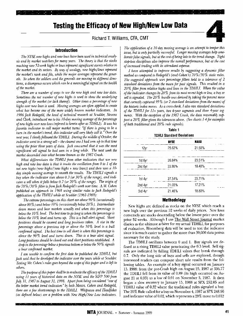
Testing the Efficacy of New High/New low Data

Richard T. Williams, CFA, CMT

Introduction The NYSE new highs and new lows have been used in technical analy-

sis and by market watchers for many years. The theory is that the stocks reaching new 52-week highs or lows rqtrresent significant arents relative to the market and its sectors. By way of analogy, new highs/lows repesent the market S rank and file, while the major averages represent the generals. So when the soldiers and the generals are moving in different direc- tions, a divergence occurs which can be a meaningful signal on the health of the market.

There are a number of ways to use the new high and new low data. Sometimes the net number of new highs is used to show the underlying strength of the market (or lack thereof). Other times a percentage of new highs over new lows is used. Mowing averages are often applied to create what has become one of the more widely known market indicators. In 1986 Jack Redegeld, the head of technical research at Scudti, Stevens and Clark, introduced me to his 1 O-day moving average of the percentage of new highs over new lows (referred to herein after as TDHLI). It was his favorite indicator to call major market turns: “If there is going to be a turn in the market’s trend, this indicator will vq likely call it. ” Over the next year, I closely followed the TDHLI. During the middle of Octobs the indicator went to a strong sell - the clearest one I had seen up to that time using the prior three years of data. Jack concurred that it was the most signaficant sell signal he had seen in a long while. The next week the market descended into what became known as the 1987 Crash.

What differentiates the TDHLI from other indicators that use new high and new low data is that it tracks the oscillationfi-om 0 to 1 of the net new highs (new highs/(new highs + new lows)) and then uses a 1 O- day simple moving average to smooth the results. The TDHLI signalr a buy when the indicator rises above 0.3 (or 30 % of the range), and indicates a sell when it falls below 0.7 (or 70 % of the range). The origin of the 70 %/30 % filter is from Jack Bedegeld ‘s work over time. A. IV Cohen published an approach in 1968 using similar rules to Jack Be&geld’s application of the TDHLI while at Scudder (1961-l 989):

The extreme percentages on this chart are above 90 % (occasionally above 80 %) and below 10% (occasionally below 20%). Intermediate down moves and bear markets usually end when this percentage is below the 10% level. The best time to go long is when the percentage is below the 10 % level and turns up. This is a bull alert signal. Short positions should be covered and long positions taken. A rise in the percentage above a previous top or above the 50% level is a bull confirmed signal. The best time to sell short is when this percentage is above the 90% level and turns down. This is a bear alert signal. Long positions should be closed out and short positions established. A drop in the percentage below apevious bottom or below the 50 % signals a bear confirmed market.

I am unable to confirm the first date he published the TDHLI, but Jack said that he developed the indicator over the years while at Scuda!er Testing Mr Cohen’s rules goes beyond the scope of this paper and is l& to others.

The purpose of thispapershall be to evaluate the efjjcaq of the TDHLI using 11 years of historical data on the NYSE and the SO-P 500 from

July 31, 1987 to August 31, 1998. Apart from being considered “one of

the better market trend indicators” by both Messrs. Cohen and Redegeld, there are a few shortcomings to the TDHLI Whipsaws and Headfakes (as defined below) are a poblem with New High/New Low indicators.

The a@lication of a lo-day moving average is an attempt to temper this issue, but is only partially successful. Longer moving averages help ame- lioratefalse signals, but at the cost of being late to the trend change. Tight stop-loss disciplines also improve the overall perfmance, but at the cost of increased trading with its attendant expense.

I have attempted to impove results by suggesting a dynamic filter method as compared to Redegeld’s (and Cohen S) 70 %/30 % static rules. The suggested a#roach uses percentage filters held to a tolerance of 2 standard deviations from the mean fw past signals. This resulted in a 20% filtufiorn relative highs and lows in the TDHLI. When the value of the indicator changes by 20 % fr om its most recent high or low, a buy or sell is signaled. The 20 % hurdle was den’ved by taking the percent move that correctly captured 95 % (or 2 standard o!eviations from the mean) of the historic index moves. As a cross-check, I also ran standard deviations of the TDHLI for ll+ years, two &year segments and three 4-year segments. With the exception of the 1987 Crash, the data reasonably sup port a 20 % filter given the tolerances above. (See charts 1-4 for examples of both traditional and 20 % rule signals).

Table 1

TDHLI Standard Deviations

HYSE WAS0

12yr 25.62% 21.50%

lst6yr 26.84% 23.51%

2nd6yr 22.80% 18.40%

lst4yr 27.54% 23.71% ----- 2nd4yr 21.03% 17.21%

3rd 4yr 21.46% 18.80%

Methodology New highs are defined as stocks on the NYSE which reach a

new high over the previous 52 weeks of daily prices. New lows conversely are stocks descending below the lowest price over the prior 52 weeks. Although I use The Wall Street Tournal market diaries as the ultimate arbiter for my actual TDHLI, for purposes of evaluation, Bloomberg data will be used to test the indicator since it is much easier to gather the more than 30,000 data points necessary for the study.

The TDHLI oscillates between 0 and 1. Buy signals are defined as a rising TDHLI value penetrating the 0.3 level. Sell signals are indicated by falling TDHLI values that break through 0.7. Only the long side of buys and sells are explored, though interested readers can compute short sale results from the following tables. An example of a buy signal occurred on January 15, 1988: from the pre-Crash high on August 25, 1987 at 336.77 the TDHLI fell from its value of 0.89 (its high occurred on Au- gust 21 at 0.93) to a low of 0.01 on November 3, 1987. It then began a slow recovery to January 15, 1988 at SPX 252.05 and TDHLI value of 0.32 where the traditional rules signaled a buy. The 20% Rule called for a buy on November 4,1987 at SPX 248.96 and indicator value of 0.02, which represents a 20% move to 0.012

MTA JOURNAL l Summer -Autumn 1999 41

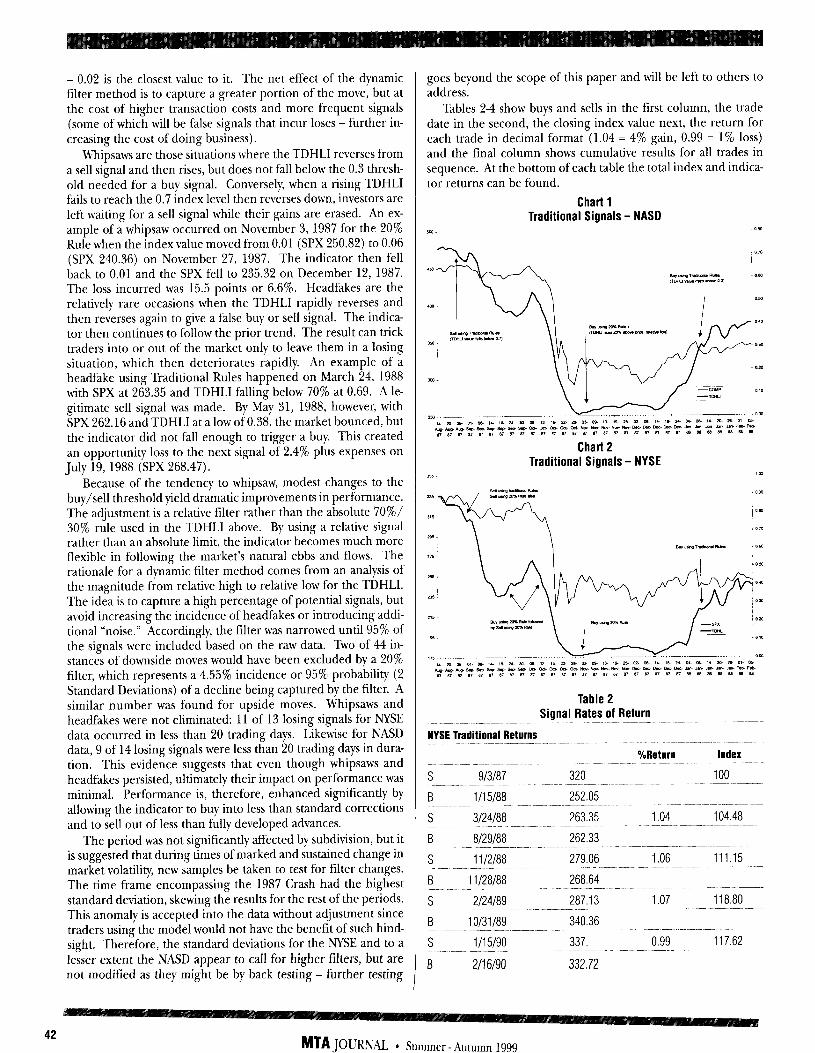
- 0.02 is the closest value to it. The net effect of the dynamic filter method is to capture a greater portion of the move, but at the cost of higher transaction costs and more frequent signals (some of which will be false signals that incur loses - further increasing the cost of doing business).

Whipsaws are those situations where the TDHLI reverses from a sell signal and then rises, but does not fall below the 0.3 threshold needed for a buy signal. Conversely, when a rising TDHLI fails to reach the 0.7 index level then reverses down, investors are left waiting for a sell signal while their gains are erased. An example of a whipsaw occurred on November 3, 1987 for the 20% Rule when the index value moved from 0.01 (SPX 250.82) to 0.06 (SPX 240.36) on November 27, 1987. The indicator then fell back to 0.01 and the SPX fell to 235.32 on December 12, 1987. The loss incurred was 15.5 points or 6.6%. Headfakes are the relatively rare occasions when the TDHLI rapidly reverses and then reverses again to give a false buy or sell signal. The indicator then continues to follow the prior trend. The result can trick traders into or out of the market only to leave them in a losing situation, which then deteriorates rapidly. An example of a headfake using Traditional Rules happened on March 24, 1988 with SPX at 263.35 and TDHLI falling below 70% at 0.69. A legitimate sell signal was made. By May 31, 1988, however, with SPX 262.16 and TDHLI at a low of 0.38, the market bounced, but the indicator did not fall enough to trigger a buy. This created an opportunity loss to the next signal of 2.4% plus expenses on July 19, 1988 (SPX 268.47).

Because of the tendency to whipsaw, modest changes to the buy/sell threshold yield dramatic improvements in performance. The adjustment is a relative filter rather than the absolute 70%/ 30% rule used in the TDHLI above. By using a relative signal rather than an absolute limit, the indicator becomes much more flexible in following the market’s natural ebbs and flows. The rationale for a dynamic filter method comes from an analysis of the magnitude from relative high to relative low for the TDHLI. The idea is to capture a high percentage of potential signals, but avoid increasing the incidence of headfakes or introducing additional “noise.” Accordingly, the filter was narrowed until 95% of the signals were included based on the raw data. Two of 44 in- stances of downside moves would have been excluded by a 20% filter, which represents a 4.55% incidence or 95% probability (2 Standard Deviations) of a decline being captured by the filter. A similar number was found for upside moves. Whipsaws and headfakes were not eliminated: 11 of 13 losing signals for NYSE data occurred in less than 20 trading days. Likewise for NASD data, 9 of 14 losing signals were less than 20 trading days in duration. This evidence suggests that even though whipsaws and headfakes persisted, ultimately their impact on performance was minimal. Performance is, therefore, enhanced significantly by allowing the indicator to buy into less than standard corrections and to sell out of less than fully developed advances.

The period was not significantly affected by subdivision, but it is suggested that during times of marked and sustained change in market volatility, new samples be taken to test for filter changes. The time frame encompassing the 1987 Crash had the highest standard deviation, skewing the results for the rest of the periods. This anomaly is accepted into the data without adjustment since traders using the model would not have the benefit of such hindsight. Therefore, the standard deviations for the NYSE and to a lesser extent the NASD appear to call for higher filters, but are not modified as they might be by back testing - further testing

goes beyond the scope of this paper and will be left to others to address.

Tables 2-4 show buys and sells in the first column, the trade date in the second, the closing index value next, the return for each trade in decimal format (1.04 = 4% gain, 0.99 = 1% loss) and the final column shows cumulative results for all trades in sequence. At the bottom of each table the total index and indicator returns can be found.

Charll Traditional Signals - NASD

Chart 2 Traditional Signals - NYSE

Table 2 Signal Rates of Return

NYSE Traditional Returns

s g/3/87 320

B l/15/88 252.05

s 3/24t88 263.35

B 8129188 262.33

s 11/2/88 279.06

B 11/28/88 268.64

s 2124189 287.13

B 10/31/89 340.36

s l/15/90 337.

B 2/i 6/90 332.72

%Return Index

100

1.04 104.48

1.06 111.15 ._~~~ .- ~. ..-

1.07 118.80

0.99 117.62

42 MTA JOURNAL * Summer-Autumn 1999

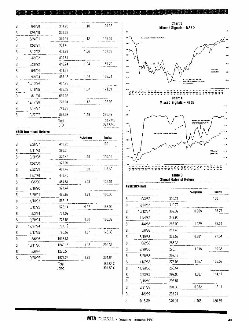
s 6/6/90 364.96 1.10 129.02

B 12/5/90 329.92

s 6124191 370.94 1.12 145.06

B 12/2/91 381.4

S 3/12/92 403.89 1.06 153.62

B 419192 400.64

S 5128192 416.74 1.04 159.79

B 515194 451.38

S g/9/94 468.18 1.04 165.74

B 10/13/94 467.79

S 2116195 485.22 1.04 171.91

B 8/l/96 650.02

S 12117196 726.04 1.12 192.02

B 4114197 743.73

S 1 O/27/97 876.98 1.18 226.42 ~~. _.-.. ~~-.--- .--~ ~~.

Total 126.42% SPX 243.57%

WAS0 Traditional Returns ---- - %Return Index

S 8126187 455.26 100

B l/11/88 336.2

S 3128188 370.42 1.10 110.18 ~--______ B 1212188 373.91

S 2122189 402.49 1.08 118.60

B 11/7/89 449.40

S 615190 464.61 1.03 122.61

B 12/l O/90 371.47

S 6120191 485.88 1.31 160.38

B 4/l 4192 588.15

S 8112192 573.14 0.97 156.92

B 513194 731.69

S 9120194 778.66 1.06 166.32

B 12127194 737.12

S 2/l 7195 790.62 1.07 178.39

B 816196 1098.81

S 10/11/96 1240.15 1.13 201.34

B 516197 1270.5

S 10128197 1671.25 1.32 264.84

Total 164.84% Comp 301.63%

Chart 3 Missed Signals - NASD

Chart 4 Missed Signals - NYSE

Table 3 Sianal Rates of Return

NYSE 20% Rule

%Return Index

s 913187 320.21 100

B 9124187 319.72

S 10/12/87 309.39 0.968 96.77

B 1114187 248.96

S 414188 256.09 1.029 99.54

B 516188 257.48 ~-~ S 5119188 252.57 0.981 97.64

B 612188 265.33 ~-._____~ S 7120188 270. 1.018 99.36

B 8125188 259.18

S 1117188 273.93 1.057 105.02

B 11128188 268.64

S 2123189 292.05 1.087 114.17 ~.~

B 3115189 296.67

S 3/21/89 291.33 0.982 112.11

B 4/5/89 296.24 _____ -~- s 9115189 345.06 1.165 130.59


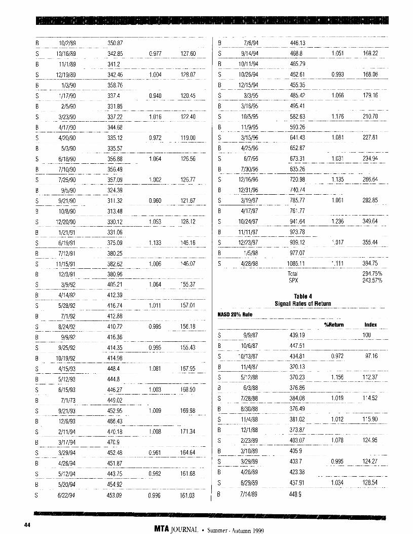
B 10/2/89 350.87

s 10/16/89 342.85 0.977 127.60

B 11/l/89 341.2

-- s 12/19/89 342.46 1.004 128.07

0.940 120.45

B 2/5/90 331.85

S 3/23/90 337.22 1.016 122.40

B 4/17/90 344.68

S 4/20/90 335.12 0.972 119.00

B 5/3/90 335.57

S 6/18/90 356.88 1.064 126.56

B 7/10/90 356.49

S 7125190 357.09 1.002 126.77

B 915190 324.39

S g/21/90 311.32 0.960 121.67

B 10/8/90 313.48

S 12/20/90 330.12 1.053 128.12

B l/21/91 331.06

S 6/19/91 375.09 1.133 145.16

B 7/12/91 380.25

S 11/15/91 382.62 1.006 146.07

B 1213191 380.96

S 319192 405.21 1.064 155.37

B 4114192 412.39

S 5128192 416.74 1.011 157.01

B 7/l I92 412.88

S 8124192 410.72 0.995 156.18

B g/9/92 416.36

S 9125192 414.35 0.995 155.43

B 10/19/92 414.98

S 4115193 448.4 1.081 167.95

B 5/12/93 444.8

S 6/15/93 446.27 1.003 168.50

B 7/l/73 449.02

S 9121193 452.95 1.009 169.98

B 1216193 466.43

S- 2/11/94 470.18 1.008 171.34

B 3/17/94 470.9

S 3/29/94 452.48 0.961 164.64

B 4126194 451.87

S 5112194 443.75 0.982 161.68 .~ ~~~~. ~~.

B 5120194 454.92

S 6122194 453.09 0.996 161.03

B 716194 446.13

S g/14/94 468.8 Iii1

B 10/11/94 465.79

S 10/26/94 462.61 0.993

B 12115194 455.35

S 313195 485.42 1.066

B 3/16/95 495.41

S 1 o/5/95 582.63 1.176

B 1119195 593.26

S 3/15/96 641.43 1.081

B 4125196 652.87

S 617196 673.31 1.031 .~ ~~~ B 7130196 635.26

S 12/16/96 720.98 1.135

B 12/31/96 740.74

S 3/19/97 785.77 1.061

B 4117197 761.77

S 10124197 941.64 1.236 ---. B 11/11/97 923.78

S 12123197 939.12 1.017

B l/5/98 977.07

S 4128198 1085.11 1.111

Total SPX

Table 4 Signal Rates of Return

NASD 20% Rule

%Return ---- S 919187 439.19

B 1016187 447.51 I_--- .- S lo/13187 434.81 0.972

B 1114187 320.13

S 5112188 370.23 1.156

B 613188 376.86

S 7128188 384.08 1.019

B 8130188 376.49

S 1114188 381.02 1.012

B 12/l/88 373.87

S 2123189 403.07 1.078

B 3/10/89 405.9

-- S 3129189 403.7 0.995 .-

B 4126189 423.38

s 6129189 437.91 1.034

B 7114189 448.9

169.22

168.06

179.16

210.70

227.81

234.94

266.64

-~ 282.85

349.64

355.44

394.75

294.75% 243.57%

Index

100

97.16

112.37

114.52

115.90

124.95

124.27

128.54

44 MTA JOURNAL * Summer - !wtumn 1999

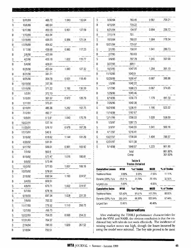
s 9/20/89 466.72 1.040 133.64

B 1 O/6/89 483.64

s lo/17189 459.93 0.951 127.09

B 11/13/89 455.94

s 12/18/89 436.03 0.956 121.54 - B 12129189 454.82

S l/17/90 438.68 0.965 117.23 ____- B 2/6/90 423.99

S 4/2/90 433.18 1.022 119.77

B 514190 428.61 -- ~~~~~~.- S 6/25/90 455.64 1.063 127.32

B 8/31/90 381.21

S g/25/90 354.78 0.931 118.49

B 10/19/90 337.36

S 12/19/90 371.22 1.100 130.39

B l/2/91 372.19

S l/10/91 361.92 0.972 126.79

B l/17/91 375.81

S 6/19/91 485.36 1.292 163.75 ____-~ B 7/12/91 492.71

S 10/g/91 513.81 1.043 170.76

B 10/22/91 537.14

s 11/20/91 526.12 0.979 167.26

B 12/13/91 540.9

S 3/16/92 618.62 1.144 191.29

B 4/20/92 591.81

S 6/17/92 569.01 0.961 183.92

B 712192 563.6 __.~~ S 8/19/92 572.47 1.016 186.81

B g/9/92 573.44

S 10/2/92 577.63 -1.007 188.18

B 10/20/92 578.64

S 2/18/92 690.54 1.193 224.57

B 314193 669.51

S 418193 670.71 1.002 224.97

B 517193 678.16

S 6/18/93 697.34 1.028 231.33

B 719193 702.22

S 11/17/93 779.32 1.110 256.73

B 1217193 766.73

S 12122193 759.23 0.990 254.22

i 12/31/93 764.57

S 2114194 786.53 1.029 261.52

B 3/l 8194 793.51

S 3/30/94 783.45 0.987 258.21

B 4115194 739.22

S 6/21/94 734.97 0.994 256.72 -~ B 7/11/74 701.

S 10/3/94 760.01 1.084 278.34

B 12/21/94 729.07

S 2/l/95 758.91 1.041 289.73

B 217195 763.63

S 3/g/95 797.78 1.045 302.68

B 3127195 809.1

S 1013195 1047.05 1.294 391.70

B 11/10/95 1043.9

S 12/20/95 1030.47 0.987 386.66

B l/3/96 1042.22

s l/17/96 1008.23 0.967 374.05

B l/29/96 1043.46

S 6/14/96 1230.73 1.179 441.18 -

B 7129196 1042.36

S 10/24/96 1236.41 1.186 523.32

B 11/14/96 1262.67

S 12/17/96 1298.33 1.028 538.09

B l/3/97 1287.75

S 313197 1340.55 1.041 560.16 _- B 4117197 1216.41

S 10127197 1708.08 1.404 786.57

B 12131197 1511.38

S 5114198 1848.07 1.223 961.80

Total 861.80% -~ Comp 301.63%

Table 5 Trades Detailed

Cumulative Losses NYSE %of Trades NASII % of Trades

Traditional Rules 0.99% 8.33% -2.55% 11.11%

Dynamic (20%) Rule -29.51% 31.70% -39.16% 32.56% -

Largest Loss -5.69% -6.93%

Cumulative Gains NYSE %of Trades WAS0 % of Trades

Traditional Rules 125.43% 91.67% 162.29% 88.89%

Dynamic (20%) Rule 265.24% 68.30% 822.64% 67.44%

Largest Gain 23.60% 40.40%

Observations After evaluating the TDHLI performance characteristics for

both the NYSE and NASD, the obvious conclusion is that the traditional buy/sell rules do not work effectively. The incidence of missing market moves was high, though the losses incurred by using the model were minimal. The buy side proved to be most

MTA JOURhN * Summer-Autumn 1999

effective after a long period of low TDHLI values. The sell side was premature, but did catch the 1987 Crash rather spectacularly in both markets.

The traditional TDHLI gives a limited number of signals. It is better on the buy side than the sell side and misses significant moves in the market. Over the test period from July 31, 1987 to September 9, 1998, there were 12 buys and 12 sells (and many sells that occurred without a prior buy signal being reached). Of the 12 signals, the TDHLI performance for the NYSE was 92.78% vs. 216% for the S&P 500. The TDHLI for the NASD had 10 buys and 10 sells. The incidence of missing meaningful moves in the COMP index was similarly significant as with the hYSE. Perfor- mance was 140.66% vs. 274% for the COMP index. The number of unrequited sell-signals for the NASD was comparable to the NYSE experience.

The signals were then adjusted to take into account incom- plete market moves. For example, the TDHLI signals a sell and then fails to reach a buy prior to the next sell signal. At times this unrequited sell signal is a prelude to a deeper correction in the averages, but it also can span months and miss large market moves. Hence, the need to adjust signal thresholds to capture partial movements in the market. In the context of this paper, a dynamic filtering method was suggested which used a confidence level of 2 standard deviations from the mean of highs and lows in the TDHLI. Based on the data, a 20% hurdle was established by cap- turing 97% of the signals while minimizing false signals. Applica- tion of the dynamic filter method is as follows: if the TDHLI reverses trend, its values are followed until they rise or fall by 20% from the prior relative high or low, thereby establishing a buy or sell signal. A relative high or low is identified after the fact by the filter rising or falling by the prescribed amount. The risk of using this type of filter in choppy markets is that multiple signals may be issued because the appropriate filter width has widened due to changing conditions. One solution that to this problem may be to track the typical number of buy/sell signals over an increment of time and use it as a flag to indicate that market conditions have changed and the filter rules need to be revisited. The duration of this study was fairly long in an attempt to address the issue of changing conditions by including a variety of market corrections and rallies. But no static filter can accommodate the dynamics of the market all the time.

Performance of the dynamic filter method for the TDHLI was stunning compared to the traditional rules. The NYSE indicator returned 294.75% vs. 243.57% for the SPX and the NASD returned a notable 861.80% vs. 301.63% for the COMP. The essential difference was that by tracking the relative movements of the TDHLI and signaling reversals of intermediate magnitude, significant moves in the market were captured by the indicator. The other feature is that buy signals jumped to 41 and 44 for NYSE and NASD respectively. Of the 41 NYSE signals, 6 were double digit returns. The largest loss was 6%. So the source of returns was a number of solid trades with one topping 24%, but only modest loses. NASD results were 11 of 44 trades (25%) breaking double digits and one over 40% while loses kept to less than 7% - the essence of a successful trading model: small loses and several outsized gains. Judging from the results of the dynamic filter method for both the NYSE and NASD histories, 14.6% and 25% of the signals respectively were substantial gains. While 13 and 15 (31.7% and 34.17) ‘g 1 o sr na s respectively lost money, none of the loses amounted to more than 8%. In my opinion, the indicated results are both robust and reliable for the dynamic filter method.

The adjustment to a dynamic filter has changed the TDHLI from an investment model into a trading model. The implica- tion being that higher trading costs, higher tax impacts on profits, more time to manage the process are required using the dynamic filter method, but not enough to discount the higher profits made by the technique. The average holding period was 61 trading days or 93 calendar days. The traditional model was 250 trading days or almost one year. The NASD average holding period was similar with 62 days vs. 305 days using traditional rules. Depending on the magnitude of gains made by the trading model over the longer term version, tax costs will be subsumed. Put a different way, to capture a 10% return using long-term capital gains tax requires at pretax profit of 12.5%. To make the same return while paying short-term capital gains tax, an 18.18% profit is required. So as long as the model can generate 45% more profit than the longer term version, investors will be better off paying the tax with the trading model.

Conclusion The traditional TDHLI failed to keep pace with the market. It

provided useful sell and buy signals under certain conditions, but cannot be considered an effective indicator on its own merits. Modest adjustments to the signal thresholds proved to be very effective. Buy and sell signals using the dynamic filter method were timely and useful, but with the potential disadvantage of increased trading costs compared to the traditional TDHLI rules. Finally, as with so many technical tools, the TDHLI cannot be used in and of itself as an indicator of market direction and magnitude. It does, however, rank among the most effective and long standing methods of technical analysis.

Attribution Redegeld, Joseph, The Ten Dav New High/New Low Index, 1986. Cohen, A. W., Three-Point Reversal Method of Point & Figure Stock Market Trading, 8th Edition, 1984, Chartcraft, Inc., pg 91. Jarrett, Dennis E., CMT, Technical Outlook, Ridder Peabody, 1994. Hayes, Timothy MT., CMT, New Highs and liew Lows, Technical Analysis Stocks & Commodities, Bonus Issue 1998, pg 40. Parker, Harold, CMT, The High-low Index as a Tool to Enhance Returns, MTA lournal, Spring-Summer 1996, pg 35. Colby, Robert W. and Meyers, Thomas A., Encvclonedia of Technical Market Indicators, pgs 304316.

Richard Williams Richard T. Williams, CFA, CMT is a Vice President and

fundamental/technical research analyst for the Convertible Se- curities Department ofJefferies & Company, Inc. He specializes in Enterprise Software/ E-commerce infrastructure stocks. Prior to joiningJefferies in 1997, Mr. Williams was an institutional sales- man at Ridder Peabody/Paine Webber from 1992 to 1996. From 1988 to 1992, he was a convertible and warrant sales trader.

Mr. Williams received his MBA in Finance from New York University.


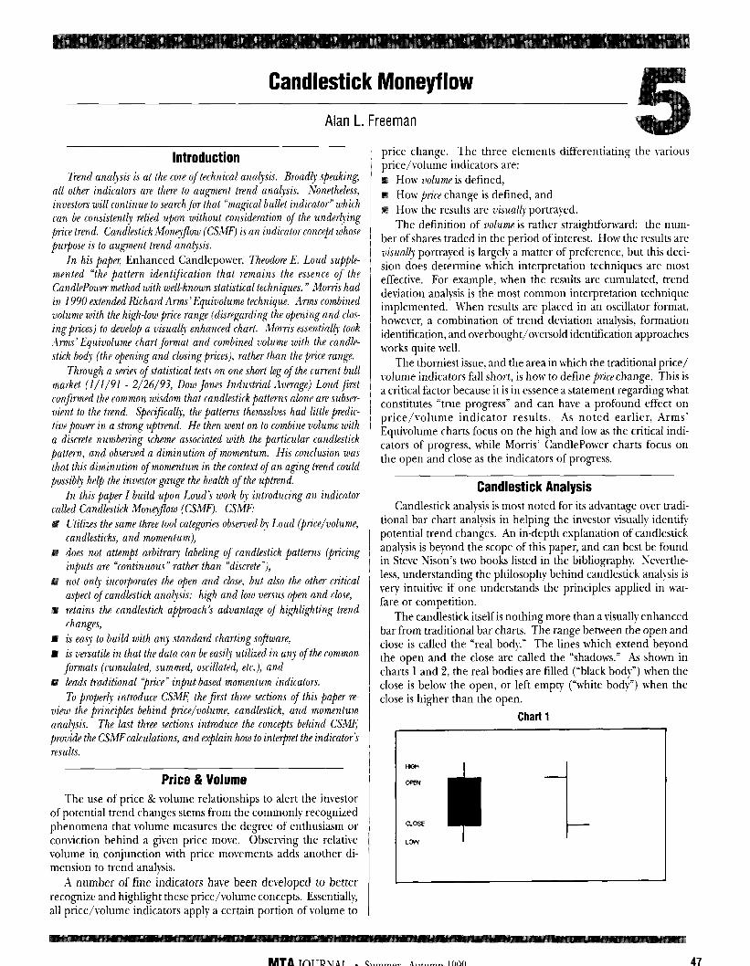
Candlestick Moneyflow

Alan L. Freeman

Introduction Trend analysis is at the cure of technical analysis. Broadly speaking

all other indicators are there to augment trend analyis. Xonetheless, investors will continue to search for that “magical bullet indicator” which can be consistently relied upon without consideration of the underl$ng price trend. Candlestick Mont$ow (CSW) is an indicator concept whose purpose is to augment trend analyis.

In his paps Enhanced Candlepower, Theodore E. Loud supple mented “the pattern identification that remains the essence of the Candlepower method with well-known statistical techniques. ” Morris had in 1990 extended Richard Arms’Equiuolume technique. Arms combined volume with the high-low price range (disregarding the opening and closing prices) to deuelop a visually enhanced chart. Xorris essentially took Arms’ Equiuolume chart format and combined volume with the candlestick body (the opening and closing prices), rather than the price range.

Through a series of statistical tests on one short leg of the current bull market (l/1/91 - 2/26/93, Dow Jones Industrial Average) Loud first confirmed the common wisdom that candlestick patterns alone are subser- Gent to the trend. Specifically, the patterns themselves had little predic- tiue power in a strong uptrend. He then went on to combine volume with a discrete numbering scheme associated with the particular candlestick pattern, and observed a diminution of momentum. His conclusion was that this diminution of momentum in the context of an aging trend could possibb help the investor-gauge the health of the uptmnd.

In this paper I build upon Loud? work by introducing an indicator called Candlestick Montyjlow (CSMF). CSMF:

Utilizes the same three tool categories observed bJ Loud (price/volume, candlesticks, and momentum),

does not attempt arbitrary labeling of candlestick patterns (pricing inputs are “continuous” rather than “discrete”),

not only incorporates the open and close, but also the other critical aspect of candlestick analysis: high and low uersus open and close,

retains the candlestick approach’s advantage of highlighting trend changes,

is easE to build with any standard charting software,

is versatile in that the data can be easily utilized in any of the common formats (cumulated, summed, oscillated, etc.), and

leads traditional “price” input-based momentum indicators.

To prop& introduce CSI~ the first three sections of this paper review the principles behind price/volume, candlestick, and momentum anal)lsis. The last three sections introduce the concepts behind CSIV& provide the CSMFcalculations, and explain how to interpet the indicator’s results.

Price & Volume The use of price & volume relationships to alert the investor

of potential trend changes stems from the commonly recognized phenomena that volume measures the degree of enthusiasm or conviction behind a given price move. Observing the relative volume in conjunction with price movements adds another dimension to trend analysis.

A number of fine indicators have been developed to better recognize and highlight these price/volume concepts. Essentially, all price/volume indicators apply a certain portion of volume to

price change. The three elements differentiating the various price/volume indicators are:

How volume is defined, How ptice change is defined, and How the results are visual4 portrayed. The definition of volume is rather straightforward: the num-

ber of shares traded in the period of interest. How the results are visually portrayed is largely a matter of preference, but this decision does determine which interpretation techniques are most effective. For example, when the results are cumulated, trend deviation analysis is the most common interpretation technique implemented. Mhen results are placed in an oscillator format, however, a combination of trend deviation analysis, formation identification, and overbought/oversold identification approaches works quite well.

The thorniest issue, and the area in which the traditional price/ volume indicators fall short, is how to define pticechange. This is a critical factor because it is in essence a statement regardingwhat constitutes “true progress” and can have a profound effect on price/volume indicator results. As noted earlier, Arms’ Equivolume charts focus on the high and low as the critical indicators of progress, while Morris’ Candlepower charts focus on the open and close as the indicators of progress.

Candlestick Analysis Candlestick analysis is most noted for its advantage over tradi-

tional bar chart analysis in helping the investor visually identify potential trend changes. An in-depth explanation of candlestick analysis is beyond the scope of this paper, and can best be found in Steve Nison’s two books listed in the bibliography. Neverthe- less, understanding the philosophy behind candlestick analysis is very intuitive if one understands the principles applied in war- fare or competition.

The candlestick itself is nothing more than a visually enhanced bar from traditional bar charts. The range between the open and close is called the “real body.” The lines which extend beyond the open and the close are called the “shadows.” As shown in charts 1 and 2, the real bodies are filled (“black body”) when the close is below the open, or left empty (“white body”) when the close is higher than the open.

Chart1

LIC I

am

LCW


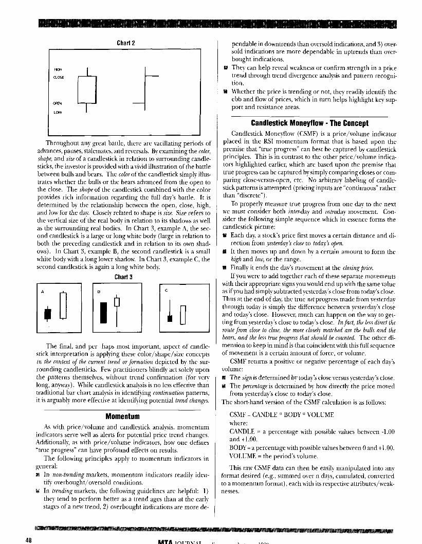
Chart 2

CLOSE

:3 lsw J

Throughout any great battle, there are vacillating periods of advances, pauses, stalemates, and reversals. By examining the calm, shape, and size of a candlestick in relation to surrounding candlesticks, the investor is provided with avivid illustration of the battle between bulls and bears. The color of the candlestick simply illustrates whether the bulls or the bears advanced from the open to the close. The shape of the candlestick combined with the color provides rich information regarding the full day’s battle. It is determined by the relationship between the open, close, high, and low for the day. Closely related to shape is size. Size refers to the vertical size of the real body in relation to its shadows as well as the surrounding real bodies. In Chart 3, example A, the second candlestick is a large or long white body (large in relation to both the preceding candlestick and in relation to its own shadows). In Chart 3, example B, the second candlestick is a small white body with a long lower shadow. In Chart 3, example C, the second candlestick is again a long white body.

Chart 3

The final, and per haps most important, aspect of candlestick interpretation is applying these color/shape/size concepts in the context of the current trend or formation depicted by the surrounding candlesticks. Few practitioners blindly act solely upon the patterns themselves, without trend confirmation (for very long, anyway). While candlestick analysis is no less effective than traditional bar chart analysis in identifying continuation patterns, it is arguably more effective at identifying potential trend changes.

Momentum As with price/volume and candlestick analysis, momentum

indicators serve well as alerts for potential price trend changes. Additionally, as with price/volume indicators, how one defines “true progress” can have profound effects on results.

The following principles apply to momentum indicators in general:

In non-trending markets, momentum indicators readily identify overbought/oversold conditions. In trending markets, the following guidelines are helpful: 1) they tend to perform better as a trend ages than at the early stages of a new trend, 2) overbought indications are more de-

pendable in downtrends than oversold indications, and 3) oversold indications are more dependable in uptrends than overbought indications. They can help reveal weakness or confirm strength in a price trend through trend divergence analysis and pattern recognition. Whether the price is trending or not, they readily identify the ebb and flow of prices, which in turn helps highlight key support and resistance areas.

Candlestick Moneyflow - The Concept Candlestick MoneyBow (CSMF) is a price/volume indicator

placed in the RSI momentum format that is based upon the premise that “true progress” can best be captured by candlestick principles. This is in contrast to the other price/volume indicators highlighted earlier, which are based upon the premise that true progress can be captured by simply comparing closes or comparing close-versus-open, etc. No arbitrary labeling of candlestick patterns is attempted (pricing inputs are “continuous” rather than “discrete”).

To properly measure true progress from one day to the next we must consider both inter-day and intraday movement. Con- sider the following simple sequence which in essence forms the

Each day, a stock’s price first moves a certain distance and direction from yesterday’s close to today’s open.

It then moves up and down by a certain amount to form the high and low, or the range. Finally it ends the day’s movement at the closing price.

If you were to add together each of these separate movements with their appropriate signs you would end up with the same value as ifyou had simply subtracted yesterday’s close from today’s close. Thus at the end of day, the true net progress made from yesterday through today is simply the difference between yesterday’s close and today’s close. However, much can happen on the way to get- ting from yesterday’s close to today’s close. In fact, the less direct the route from close to close, the more closely matched are the bulls and the bears, and the less true progress that should be counted. The other dimension to keep in mind is that coincident with this full sequence of movement is a certain amount of force, or volume.

CSMF returns a positive or negative percentage of each day’s volume:

The sign is determined by today’s close versus yesterday’s close. The percentage is determined bv how directly the price moved from yesterday’s close to today’s close.

The short-hand version of the CSMF calculation is as follows:

CSMF = CANDLE * BODY * VOLUME where: CAh’DLE = a percentage with possible values between -1.00 and t1.00. BODY = a percentage with possible values between 0 and tl.OO. VOLUME = the period’s volume.

This raw CSMF data can then be easily manipulated into any format desired (e.g., summed over n days, cumulated, converted to a momentum format), each with its respective attributes/weaknesses.

48 MTA JOURNAL l Summer - Xutumn 1999

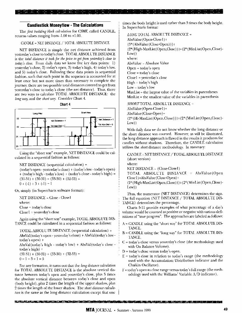
Candlestick Moneyflow - The Calculations The first building block calculation for CSMF, called CANDLE,

returns values ranging from -1.00 to t1.00.

CXNDLE = NET DISTAXE / TOTAL ABSOLUTE DISTANCE

NET DISTANCE is simply the net distance achieved from yesterday’s close to today’s close. TOTAL ABSOLUTE DISTANCE is the total distance it took for the price to get from yesterda)‘s close to todq’s close. From daily data we know five key data points: 1) yesterday’s close, 2) today’s open, 3) today’s high, 4) today’s low, and 5) today’s close. Following these data points in sequential fashion, such that each point in the sequence is accounted for at least once but not more times than necessary to complete the journey, there are two possible total distances covered to get from yesterday’s close to today’s close (the net distance). Thus, there are two ways to calculate TOTAL ABSOLUTE DISTAlICE: the long way, and the short way Consider Chart 4.

Chart4

Long my shortway

33 \, NeiDlrtm-c*=1

Tol*cist=5 32

31

30

Using the “short way” example, NET DISTANCE could be calculated in a sequential fashion as follows:

NET DISTANCE (sequential calculation) = (today’s open - yesterday’s close) t (today’s low - today’s open) t (today’s high - today’s low) t (today’s close - today’s high) = (31-31) t (30-31) t (33-30) t (32-33) = 0 t (-1) t 3 t (-1) = 1

Or, simply (in Supercharts software format):

NET DISTANCE = Close - Close1 where: Close = today’s close Close1 = yesterday’s close

Again using the “short way” example, TOTAL ABSOLUTE DIS- TANCE could be calculated in a sequential fashion as follows:

TOTAL ABSOLUTE DISTANCE (sequential calculation) = AbsV’al (today’s open - yesterday’s close) t AbsVal (today’s low - today’s open) t AbsVal(today’s high - today’s low) t AbsVal(today’s close - today’s high) = (31-31) t (30-31) t (33-30) t (32-33) = Otlt3tl=5

For any formation, it turns out that the long distance calculation for TOTAL ABSOLUTE DISTANCE is the absolute vertical distance between today’s open and yesterday’s close, plus 3 times the absolute vertical distance between today’s close and open (body height), plus 2 times the length of the upper shadow, plus 2 times the length of the lower shadow. The short distance calculation is the same as the long distance calculation except that one

times the body height is used rather than 3 times the body height. In Supercharts format:

LONG TOTAL ABSOLUTE DISTANCE = AbsValue(Open-Closel)t (3*(AbsValue(Close-0pen)))t (2*(High-MaxList(Open,Close)))t(2*(MinList(Open,Close)- LOWI ) where: AbsValue = Absolute Value Open = today’s open Close = today’s close Close1 = yesterday’s close High = today’s high Low = today’s low MaxList = the largest value of the variables in parentheses MinList = the smallest value of the variables in parenthesis

SHORTTOTAL ABSOLUTE DISTANCE = AbsValue (Open-Closel) t AbsValue (Close-Open) t (2*(Hi-MaxList(Open,Close)))t(2~(MinList(Open,Close)-

Low) 1

With daily data we do not know whether the long distance or the short distance was covered. However, as will be illustrated, the long distance approach is flawed in the results it produces for candles without shadows. Therefore, the CANDLE calculation utilizes the short distance methodology. In summary:

CANDLE = NET DISTANCE / TOTAL ABSOLUTE DISTANCE (short version) where: NET DISTANCE = (Close-Closel) TOTAL ABSOLUTE DISTANCE = AbsValue (Open Closel) tAbsValue (Close-Open) t (2*(High-MaxList(Open,Close)))t(2*(MinList(Open,Close)- LowI 1

Thus, the numerator (NET DISTANCE) determines the sign. The full equation (NET DISTANCE / TOTAL ABSOLUTE DIS TANCE) determines the percentage.

Charts 511 provide examples of what percentage of a day’s volume would be counted as positive or negative with various definitions of “true progress”. The approaches are labeled as follows:

A = CANDLE using the “short way” for TOTAL ABSOLUTE DIS- TANCE.

B = CANDLE using the “long way” for TOTAL ABSOLUTE DIS TANCE.

C = today’s close versus yesterday’s close (the methodology used with On Balance Volume).

D = today’s close versus today’s open. E = today’s close in relation to today’s range (the methodology

used with the Accumulation/Distribution indicator and the Chaikin Oscillator).

F = today’s open to close range versus today’s full range (the methodology used with the M’illiams’ V’ariable A/D indicator).

MTA JOCRSAL l Summer-Autumn 1999 49

Chart5

t 9

Corbuation Pattern A= 1 /(0+1+2+2) =li3=+0.20

8 B= , *0+3+2+21 = 1 R = +0.14

Chart7

/lO t

9 Cwtinuation Pattern A= 21(1 +l +O+O) = +1 .oo

a (Separating Lines) B= 2Jy1+3+0+0) = +o.xl **

7 c= +I .oo

6 D= +I .oo

5 l-l F= +I .I0

1;i Note: Lack of shaddws suggests aI1 Of

Chart8

t

Chart9

5

4- 3-

!

1

1

E= 112 = +oso

F= - 1/4 = -0.25 **

Note: C incorrectly courrts aI Of r volume. The color of a hanging man is

inmaterial, yet D 8 F switch s!gns --

from Chart 8 to 9.

Chart10

0 t

9 Reversal Pattern A= -1/(2+1+0+0)=-i ~3 = -0.33

6 (Hararni) 8= -11(2+3+0+0)=-l 5 = -0.20

7 I c= -1 .oo 6 I

D= +I .oo **

E= +I .oo **

F= +I .oo *’

Note: D, E, 8 F each would award a postive 100% of the day’s volume in --

this reversal pattern.

Chart11

As illustrated, CANDLE captures well the candlestick concepts of body size in relation to the full candle and net progress from period to period. CAXDLE does not, however, capture the concept of body size in relation to surrounding body sizes. For example, Chart 12 illustrates two candlestick formations where candle size relative to surrounding candles is a critical factor in identifying the formations.

Chart12

MTA JOL’RSL * Summer -Autumn 1999

To address this issue, the second building block calculation for CSMF, BODY, was developed. BODY is essentially the size of today’s body size as a percentage of the largest body size over the past n days. If today’s body is the largest over the past n days, then the result would be 1.00. The possible range is 0 to 1.00.

BODY = ((Today’s Body High/Today’s Body Low)-1) / (Longest Over Past n Days ((Body High/Body Low)-1))

In Supercharts format:

BODY = IFF( (Highest ( (Maxlist( Open,Close) /Minlist (Open,Close)-l),Length))=O,O, ((Maxlist(Open,Close)/ Minlist(Open,Close))-1) / (Highest( (Maxlist(Open,Close)/ Minlist(Open,Close)-l),Length)))

The logical “IFF” formulation is used simply to avoid division- by-zero errors. In Supercharts format, “Length” designates the number of days to consider for determining the largest bodysize (“Highest”). The exact number of days to consider is a matter of preference. Obviously, the shorter the time period chosen the more volatile the results will be. I prefer less volatile results and use 28 days for “Length.”

We now have the two building block calculations for CSMF, CANDLE and BODY These two factors are multiplied together, resulting in a possible range of -1 .OO to 1 .OO. Chart 13 is an illustration of CANDLE multiplied by BODY (labeled CSMFexVOL in this illustration).

Chart13

Consistent with basic candlestick principles, note that the clearer the net progress upward (open at or higher than prior close, close greater than prior close, large white body, and no shadows), the closer the value approaches 1 .OO. The clearer the net progress downward (open at or lower than prior close, close less than prior close, large black body, and no shadows), the closer the value approaches negative 1.00. Less clear net progress (e.g., shadows, or smaller bodies in relation to prior bodies) results in positive or negative values less than 1.00. In other words, the CTAh!DLE*BODY calculation captures the spirit of candlestick analysis and is a measure of true progress.

For the final step in CSMF, this level of “true progress” is then multiplied by volume:

CSMF = CANDLE * BODY(Length) * VOLUME where: Length = 28

Chart 14 illustrates CSMF in histogram format (labeled CSMFBAR in this illustration).

Chart14

As mentioned, CSMF can now be manipulated to one’s preference (summed, cumulated, etc.). For example, Chart 15 shows CSMF in cumulated format (labeled CUMCSMF) overlaid with On Balance Volume.

Chart15 CuytJyT 4wym

c.c 07 Rb Mn 41 a

The real advantage of CSMF , however, is in its enhancement of the traditional RSI indicator. There are numerous ways to con- vert the raw CSMF data, such as cumulating over the entire data series or summing over n days. However, through experimenta- tion I have found that the best results are derived from smoothing the raw data with an exponential moving average. The chal- lenge with smoothing these volatile data lies in striking a balance between a) sensitivity to the data and b) smoothness so that the indicator is workable. To smooth the data satisfactorily with one moving average requires a relatively long time period which results in too much of a “lagged” effect. Therefore, to smooth the data but minimize the lag effect, I use two shorter term exponential moving averages. Specifically, I recommend a ‘i-day exponential average of the 7day exponential average of the raw CSMF data. This smoothed data is then used as the “price” input in the RSI Formula. The time period I use for RSI is 14 days.

MTA JOURNAL l Summer -Autumn 1999 51

The formula for converting CSMF into the RSI format using Supercharts syntax is as follows:

CSMF in RSI format (or CSMFrsi) = RSI(Xaverage(Xaverage(CSMF(Length)Avlen1)Avlen2),Rsilen) where: CSMF = Supercharts user function previously defined by the C.UMF formula. Xaverage = exponential moving average. Avlenl = 7 (days length for CSMF moving average). Avlen2 = 7 (days length for moving average of Avlenl). Length = 28 (days length for relative body size calculation, “BODY) Rsilen = 14 (days length for RSI calculation)

Candlestick Moneyflow - Interpretation in RSI Format The primary advantage of using CSMF in the RSI format

(CSMFrsi) is that it is more sensitive to potential trend changes than the traditional RSI, thus it typically leads the traditional RSI chart formation. To illustrate this, Charts l&18 compare CSMFrsi to commonly used versions of RSI utilizing Close, Average Price, and Weighted Close respectively. CSMFrsi is illustrated with the dark line, while traditional RSI is illustrated with the lighter line.

Chart 16 (RSI using Close)

Chart 17 (RSI using Average Price)

Chart 18 (RSI using Weighted Close)

Charts 19-21 provide additional examples CSMFrsi versus traditional RSI utilizing the closing price.

Chart 19

MTA JOURNAL. * Summer-Autumn 1999

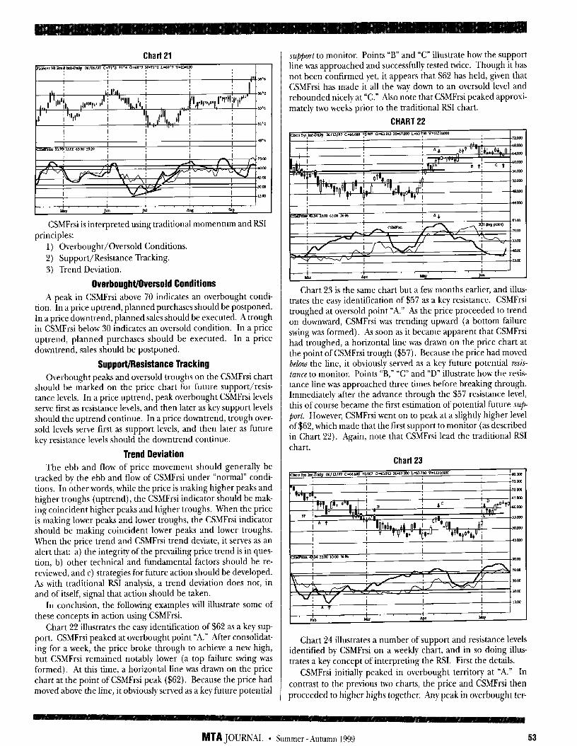
Chart21

CSMFrsi is interpreted using traditional momentum and RSI principles:

1) Overbought/Oversold Conditions. 2) Support/Resistance Tracking. 3) Trend Deviation.

Overbought/Oversold Conditions A peak in CSMFrsi above 70 indicates an overbought condi-

tion. In a price uptrend, planned purchases should be postponed. In a price downtrend, planned sales should be executed. A trough in CSMFrsi below 30 indicates an oversold condition. In a price uptrend, planned purchases should be executed. In a price downtrend, sales should be postponed.

Support/Resistance Tracking Overbought peaks and oversold troughs on the CSMFrsi chart

should be marked on the price chart for future support/resistance levels. In a price uptrend, peak overbought CSMFrsi levels serve first as resistance levels, and then later as key support levels should the uptrend continue. In a price downtrend, trough oversold levels serve first as support levels, and then later as future key resistance levels should the downtrend continue.

Trend Deviation The ebb and flow of price movement should generally be

tracked by the ebb and flow of CSMFrsi under “normal” conditions. In other words, while the price is making higher peaks and higher troughs (uptrend), the CSMFrsi indicator should be making coincident higher peaks and higher troughs. When the price is making lower peaks and lower troughs, the CSMFrsi indicator should be making coincident lower peaks and lower troughs. When the price trend and CSMFrsi trend deviate, it serves as an alert that: a) the integrity of the prevailing price trend is in question, b) other technical and fundamental factors should be re- reviewed, and c) strategies for future action should be developed. As with traditional RSI analysis, a trend deviation does not, in and of itself, signal that action should be taken.

In conclusion, the following examples will illustrate some of these concepts in action using CSMFrsi.

Chart 22 illustrates the easy identification of $62 as a key support. CSMFrsi peaked at overbought point “A.” After consolidating for a week, the price broke through to achieve a new high, but CSMFrsi remained notably lower (a top failure swing was formed). At this time, a horizontal line was drawn on the price chart at the point of CSMFrsi peak ($62). Because the price had moved above the line, it obviously served as a key future potential

support to monitor. Points “B” and “C” illustrate how the support line was approached and successfully tested twice. Though it has not been confirmed yet, it appears that $62 has held, given that CSMFrsi has made it all the way down to an oversold level and rebounded nicely at “C.” Also note that CSMFrsi peaked approximately two weeks prior to the traditional RSI chart.

CHART22

Chart 23 is the same chart but a few months earlier, and illustrates the easy identification of $57 as a key resistance. CSMFrsi troughed at oversold point “A.” As the price proceeded to trend on downward, CSMFrsi was trending upward (a bottom failure swing was formed). As soon as it became apparent that CSMFrsi had troughed, a horizontal line was drawn on the price chart at the point of CSMFrsi trough ($57). Because the price had moved below the line, it obviously served as a key future potential resistance to monitor. Points “B,” “C” and “D” illustrate how the resistance line was approached three times before breaking through. Immediately after the advance through the S57 resistance level, this of course became the first estimation of potential future su$- port. However, CSMFrsi went on to peak at a slightly higher level of $62, which made that the first support to monitor (as described in Chart 22). Again, note that C%MFrsi lead the traditional RSI chart.

Chart23

Chart 24 illustrates a number of support and resistance levels identified by CSMFrsi on a weekly chart, and in so doing illustrates a key concept of interpreting the RX First the details.

CSMFrsi initially peaked in overbought territory at “A.” In contrast to the previous two charts, the price and CSMFrsi then proceeded to higher highs together. Any peak in overbought ter-


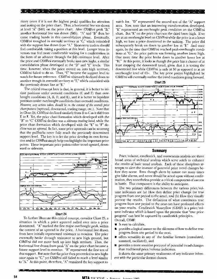
ritory (even if it is not the highest peak) qualifies for attention and noting on the price chart. Thus, a horizontal line was drawn at level “A” ($40) on the price chart. After CSMFrsi peak “B,” another horizontal line was drawn ($45). “A” and “B” then became trading bands in this consolidation phase. Eventually, CSMFrsi troughed in oversold territory at “C,” which coincided with the support line drawn from “A.” Short-term traders should feel comfortable taking a position at this level. Longer term investors may feel more comfortable waiting for a confirmation in the form of an advance through the $45 resistance level. After the price and CSMFrsi eventually broke into new highs, a similar consolidation phase developed at the “D” and “E” levels. This time, however, when the price moved on into high territory, CSMFrsi failed to do so. Thus, “E” became the support level to watch for future reference. CSMFrsi ultimately declined down to another trough in oversold territory at “F,” which coincided with the previously drawn line at “E.”

The critical concept here is that, in general, it is better to ini- tiate positions under oversold conditions (C and F) than overbought conditions (A, B, D, and E), and it is better to liquidate positions under overbought conditions than oversold conditions. Howeuer~ any action taken should be in the context of the overall price chartpattern (uptrend, downtrend, trading range, etc.). Note that in Chart 24, CSMFrsi declined similarly from B to C as it did from E to E Yet, the price chart formation which developed with the “B” to “C” CSMFrsi decline was a sideways trading band, while the price chart formation which developed with the “E” to “F” decline was an upend. In fact, some price uptrends can be so strong that the pullbacks never fully reach the previously determined support level. The key is to let the price develop its own formation and let CSMFrsi simply help you highlight the important price points. These important price points either trend upward, downward or sideways.

Chart24 To further illustrate this critical concept, consider Chart 25, a

situation in which a price uptrend rolled over into a price downtrend. “A” marked the first major overbought peak, within the context of an uptrend in the price. A horizontal line drawn from here initially represented resistance to monitor. The price eventually broke through resistance to new high ground, but CSMFrsi did not move back up into high territory. Thus, the horizontal line drawn from peak “A” on the price chart became a future support level to monitor. “B” represented the first test of that support. But note that the price then proceeded to new highs once again to “C,” yet CSMFrsi still failed to reach a level similar to “A.” At this point, therefore, “A” remained the key support to

watch for. “D” represented the second test of the “A” support area. Now, note that an interesting transformation developed. “E” represented an overbought peak condition on the CSMFrsi chart. But “E” on the price chart was the third lower high. If we are at an overbought level on CSMFrsi while the price is at a lower high, we have a price downtrend in the making. The price did subsequently break on down to another low at “F.” And once again, by the time that CSMFrsi reached peak-overbought conditions at “G,” the price pattern was forming another lower high. One more time the price broke down to another lower low at “H.” At this point, it looks as though the price has a chance of at least stopping the downward trend, given that it is testing the downtrend line while CSMFrsi is only at 50 as opposed to at an overbought level of 65t. The key price points highlighted by CSMFrsi will eventually outline the trend condition going forward.

Chart25

Summary Price/volume, candlestick, and momentum analysis are three

broad areas of technical analysis which serve solely to enhance the results of basic trend analysis. Each of these disciplines attempts to alert the investor of potential price trend changes before they occur. Even though alerts by nature can many times give false alarms, and never should be acted upon without confirmation, they nonetheless provide a critical component of success in battle. That component is the ability to anticipate.

The two primary differences between the various price/volume indicators are (a) How they define price change (or true progress from one period to the next), and (b) How they visually portray the results. The definition of what constitutes true progress from one period to the next can have profound effects on your results. Candlestick Moneyflow (CSMF) is a price/volume indicator which is based upon the premise that “true price progress” can best be captured by candlestick principles. Overall, CSMF:

Is easy to calculate, provides a logical answer to the dilemma of how to define true progress from one period to the next, offers versatility in any of the familiar formats (cumulated, summed, oscillated), and provides a more sensitive portrayal of potential trend changes than traditional price/volume indicators. It shares the same primary weaknesses of any indicator inher-

ent with the particular format chosen.


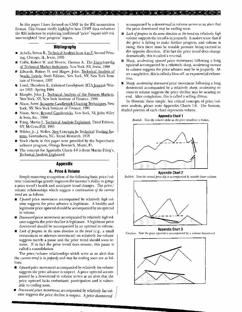
In this paper I have focused on CSMF in the RSI momentum format. This format vividly highlights how CSMF data enhances the RSI indicator by replacing traditional “price” inputs with volume-weighted “true progress” inputs.

Bibliography Achelis, Steven B., Technical Analvsis from A to Z, Second Print- ing, Chicago, IL, Irwin, 1995 Colby, Robert m7. and Meyers, Thomas A., The Encvclooedia of Technical Market Indicators, New York, NY, Irwin, 1988 Edwards, Robert D. and Magee, John, Technical Analvsis of Stocks Trends, Sixth Edition, New York, rUY, New York Insti- tute of Finance, 1992 Loud, Theodore E., Enhanced Candlepower, MTA Iournal/Win- ter 1993 - Spring 1994 Murphy, John J., Technical Analvsis of the Futures Markets, New York, NY, New York Institute of Finance, 1986 Nison, Steve,JaDanese Candlestick Charting Techniaues, New York, W, New York Institute of Finance, 1991 Nison, Steve, Bevond Candlesticks, New York, NY, John Wiley & Sons, Inc., 1994 Pring, Martin J., Technical Analvsis Exnlained, Third Edition, NY, McGraw-Hill, 1991 Wilder, Jr., J. Welles, New Concents In Technical Trading Svs- terns Greensboro, XC, Trend Research, 1978 -, Stock charts in this paper were provided by the Supercharts software program, Omega Research, Miami, FL The concept for Appendix Charts 1-8 is from Martin Pring’s, Technical Analvsis ExDlained

Appendix

A. Price 81 Volume Simply mastering recognition of the following basic price/vol-

ume relationships greatly improves the investor’s ability to gauge a price trend’s health and anticipate trend changes. The price/ volume relationships which suggest a continuation of the current trend are as follows:

CTpward price movement accompanied by relatively high volume suggests the price advance is legitimate. A healthy and legtimate price uptrend should be accompanied by an uptrend in volume. Downward price movement accompanied by relatively high volume suggests the price decline is legitimate. A legitimate price downtrend should be accompanied by an uptrend in volume. Lack of progress in the same direction as the trend (e.g., a small retracement or sideways movement) on relatively low volume suggests merely a pause and the prior trend should soon resume. If in fact the prior trend does resume, this pause is called a consolidation. The price/volume relationships which serve as an alert that

the current trend is in jeopardy and may be ending soon are as fol- ws:

Upward price movement accompanied by relatively low volume suggests the price advance is suspect. A price uptrend accompanied by a downtrend in volume serves as an alert that the price uptrend lacks enthusiastic participation and is vulner- able to ending soon.

m Downward price movement accompanied by relatively low ~01~ “me %FS~ the price decline is suspect. A price doh,ntrend 1

accompanied by a downtrend in volume serves as an alert that the price downtrend may be ending soon. Lack of popess in the same direction as the trend on relatively high volume suggests the trend is in jeopardy. It makes sense that if the price is failing to make further progress, and volume is rising, then there must be notable pressure being exerted in the opposite direction. If in fact the price trend does change dramatically, this is called a reversal. Sharp, accelerating upward price movement following a long uptrend accompanied by a relatively sharp, accelerating increase in volume suggests the price advance may be in jeopardy. Af- ter completion, this is called a blow-off, or exponential exhaustion. Sharp, accelerating downward price movement following a long downtrend accompanied by a relatively sharp, accelerating increase in volume suggests the price decline may be nearing an end. After completion, this is called a selling climax. To illustrate these simple, but critical concepts of price/vol-

ume analysis, please note Appendix Charts 1-8. The bottom, shaded portion of each chart represents volume.

Appendix Chart 1 Bearish. Note the volume spike as the price trendline is broken.

Appendix Chart 2 Bullish. Note the second price dip is accompanied bJ notab{y lower volume.

L Appendix Chart 3

Caution. Note the price uptrend is accompanied bJ a uolume downtrend.

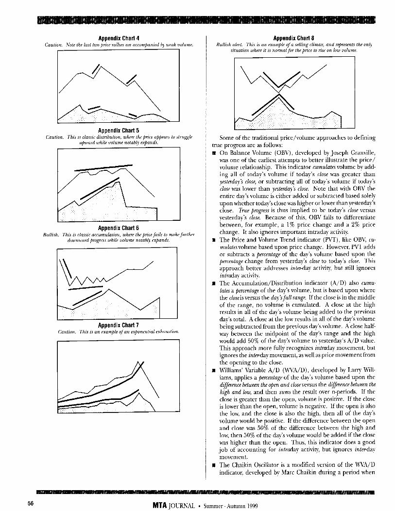
Appendix Chart 4 Caution. Note the last two price rallies are acrompanied by weak volume.

Appendix Chart 5 Caution. This is classic distribution, where theprice appears to struggle

upward while volume notably expands.

Appendix Chart 6 Bullish. This is classic accumulation, where the price fails to make further

downward progress while volume notably expands.

s J Appendix Chart 7

Caution. This is an example of an exponential exhaustion.

Appendix Chart 8 Bullish alert. This is an example of a selling climax, and rqtmwnts the only

situation where it is nmmalfor the price to rise on low volume.

Some of the traditional price/volume approaches to defining true progress are as follows:

On Balance Volume (OBV), developed by Joseph Granville, was one of the earliest attempts to better illustrate the price/ volume relationship. This indicator cumulates volume by adding all of today’s volume if today’s close was greater than ~esterda~‘s close, or subtracting all of today’s volume if today’s close was lower than pesterday’s close. Note that with OBV the entire day’s volume is either added or subtracted based solely upon whether today’s close was higher or lower than yesterday’s close. True progress is thus implied to be today’s close versus yesterday’s close. Because of this, OBV fails to differentiate between, for example, a 1% price change and a 2% price change. It also ignores important intraday activity. The Price and Volume Trend indicator (PVT), like OBV, cumulates volume based upon price change. However, PVT adds or subtracts a percentage of the day’s volume based upon the percentage change from yesterday’s close to today’s close. This approach better addresses inter-day activity, but still ignores in&day activity. The Accumulation/Distribution indicator (A/D) also cumulates a percentage of the day’s volume, but is based upon where the closeis versus the daJ ‘sfull range. If the close is in the middle of the range, no volume is cumulated. A close at the high results in all of the day’s volume being added to the previous day’s total. A close at the low results in all of the day’s volume being subtracted from the previous day’s volume. A close halfway between the midpoint of the day’s range and the high would add 50% of the day’s volume to yesterday’s A/D value. This approach more fully recognizes intraday movement, but ignores the in&day movement, as well as price movement from the opening to the close. Williams’ Variable A/D (WVA/D) , developed by Larry Will- iams, applies a percentage of the day’s volume based upon the difference between the open and closeversus the dijjfmence between the high and low, and then sums the result over n-periods. If the close is greater than the open, volume is positive. If the close is lower than the open, volume is negative. If the open is also the low, and the close is also the high, then all of the day’s volume would be positive. If the difference between the open and close was 50% of the difference between the high and low, then 50% of the day’s volume would be added if the close was higher than the open. Thus, this indicator does a good job of accounting for intraday activity, but ignores inter-day movement. The Chaikin Oscillator is a modified version of the M’VA/D indicator, developed by Marc Chaikin during a period when


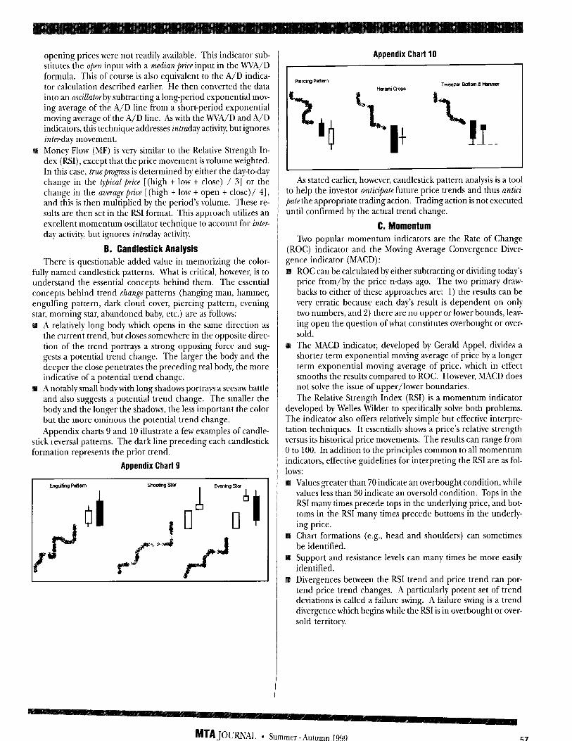
opening prices were not readily available. This indicator sul stitutes the open input with a median pice input in the WVA/ formula. This of course is also equivalent to the A/D indic tor calculation described earlier. He then converted the da1 into an oscillatorby subtracting a long-period exponential mo ing average of the A/D line from a short-period exponenti; moving average of the A/D line. As with the WVA/D and A/ indicators, this technique addresses intruday activity, but ignore inter-day movement. Money Flow (MF) is very similar to the Relative Strength Ii dex (RSI), except that the price movement is volume weightec In this case, trwfwogress is determined by either the day-to-d: change in the typical price [(high t low t close) / 31 or th change in the average price [(high t low t open t close)/ 4 and this is then multiplied by the period’s volume. These t-l sults are then set in the RSI format. This approach utilizes a excellent momentum oscillator technique to account for into day activity, but ignores intraday activity.

B. Candlestick Analysis There is questionable added value in memorizing the co10

fully named candlestick patterns. What is critical, however, is t understand the essential concepts behind them. The essenti; concepts behind trend change patterns (hanging man, hamme engulfing pattern, dark cloud cover, piercing pattern, evenin star, morning star, abandoned baby, etc.) are as follows:

A relatively long body which opens in the same direction 2 the current trend, but closes somewhere in the opposite dire1 tion of the trend portrays a strong opposing force and sul gests a potential trend change. The larger the body and th deeper the close penetrates the preceding real body, the mor indicative of a potential trend change. A notably small body with long shadows portrays a seesaw battl and also suggests a potential trend change. The smaller th body and the longer the shadows, the less important the colt but the more ominous the potential trend change. Appendix charts 9 and 10 illustrate a few examples of candle

stick reversal patterns. The dark line preceding each candlestic formation represents the prior trend.

Appendix Chart 9

b D a- ta. V- al D ‘S

;r

LV

le

I, e- n 7-

e e n- I

Appendix Chart 10

As stated earlier, however, candlestick pattern analysis is a tool to help the investor anticipate future price trends and thus anticipate the appropriate trading action. Trading action is not executed until confirmed by the actual trend change.

C. Momentum Two popular momentum indicators are the Rate of Change

(ROC) indicator and the Moving Average Convergence Diver- gence indicator (MACD) :

ROC can be calculated by either subtracting or dividing today’s price from/by the price n-days ago. The two primary draw- backs to either of these approaches are: 1) the results can be very erratic because each day’s result is dependent on only two numbers, and 2) there are no upper or lower bounds, leaving open the question of what constitutes overbought or oversold. The MACD indicator, developed by Gerald Appel, divides a shorter term exponential moving average of price by a longer term exponential moving average of price, which in effect smooths the results compared to ROC. However, MACD does not solve the issue of upper/lower boundaries. The Relative Strength Index (RSI) is a momentum indicator

developed by Welles Wilder to specifically solve both problems. The indicator also offers relatively simple but effective interpretation techniques. It essentially shows a price’s relative strength versus its historical price movements. The results can range from 0 to 100. In addition to the principles common to all momentum indicators, effective guidelines for interpreting the RSI are as fol-

ws: Values greater than 70 indicate an overbought condition, while values less than 30 indicate an oversold condition. Tops in the RSI many times precede tops in the underlying price, and bottoms in the RSI many times precede bottoms in the underlying price. Chart formations (e.g., head and shoulders) can sometimes be identified. Support and resistance levels can many times be more easily identified. Divergences between the RSI trend and price trend can por- tend price trend changes. A particularly potent set of trend deviations is called a failure swing. A failure swing is a trend divergence which begins while the RN is in overbought or oversold territory.

MTA JOURNAL * Summer -Autumn I999

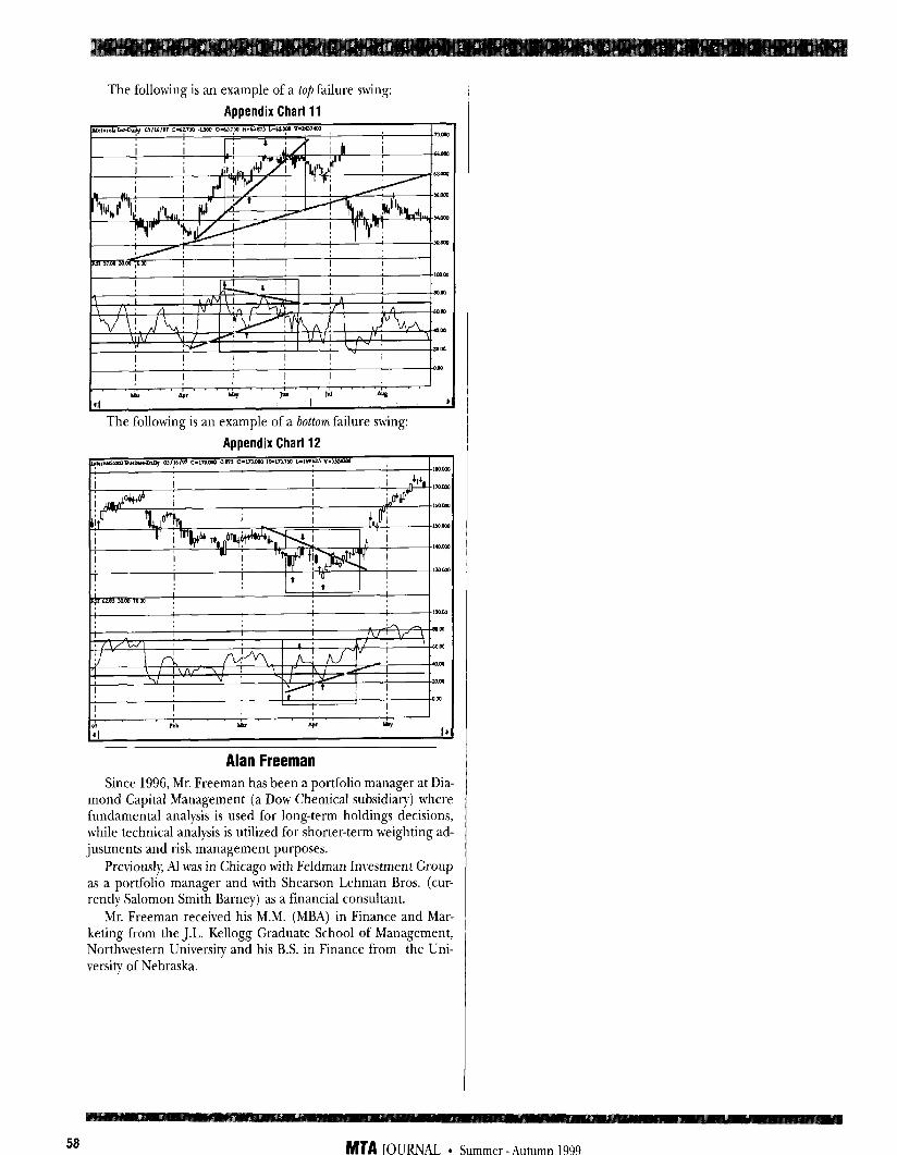
The following is an example of a top failure swing:

Appendix Charlll

m! w m P I p

4 11 ,

The following is an example of a bottom failure swing:

Appendix Chart 12

Alan Freeman Since 1996, Mr. Freeman has been a portfolio manager at Dia-

mond Capital Management (a Dow Chemical subsidiary) where fundamental analysis is used for long-term holdings decisions, while technical analysis is utilized for shorter-term weighting adjustments and risk management purposes.

Preyiously, Al was in Chicago with Feldman Investment Group as a portfolio manager and with Shearson Lehman Bras. (currently Salomon Smith Barney) as a financial consultant.

Mr. Freeman received his M.M. (MBA) in Finance and Mar- keting from the J.L. Kellogg Graduate School of Management, Northwestern University and his B.S. in Finance from the Uni- versity of Nebraska.


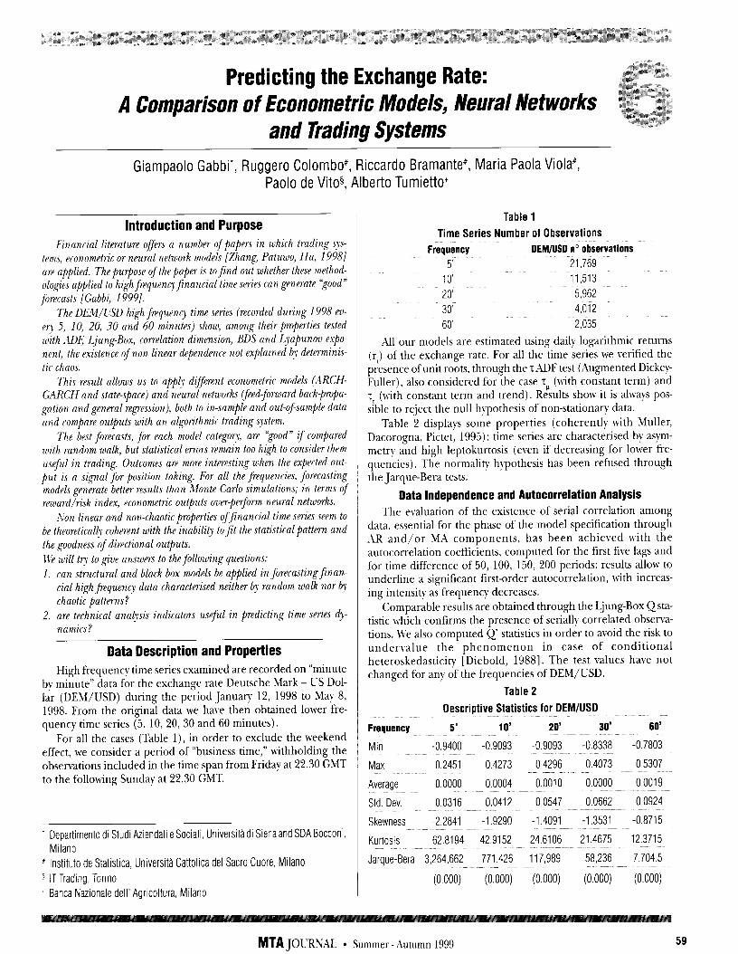
Giampaolo Gabbi’, Ruggero Colombo#, Riccardo Bramante#, Maria Paola Viola”, Paolo de Vitog, Albert0 Tumietto’

Introduction and Purpose Financial literature o&s a number of papers in which trading SJS-

terns, econometric or neural network models [Zhang, Patuwo, Hu, 19981 are applied. The purpose of the paper is to find out whether these method- olog’es applied to high frequeng finanrial time series can generate “‘good”

forecasts [Gabbi, 19991.

The DEM/C!SD high frequency time series (recorded during 1998 pu- cry 5, 10, 20, 30 and 60 minutes) shour, among their properties tested with ADE I,jung-Box, correlation dimension, BDS and Qapunou exponent, the existence of non linear dapendenre not explained ky deterministic chaos.

This result allows us to a$$$~ dijjf erent econometric models (,IRCH- GARCH and state-space) and neural networks (feed-fonuard back$ropa- Ration and general regression), both to in-sample and out-of-sum@ data and compare outputs with an algorithmic trading ytem.

The best forecasts, for each model category, are ‘&ood” if compared with random walk, but statistical errors remain too high to consider them useful in trading. Outcomes are more interesting when the expected output is a signal for position taking. For all the frequencies, forecasting models generate better results than i\lonte Carlo simulations; in terms of reward/lisk index, econometric outputs over-perform neural networks.

Xon linear and non-chaotic properties offinancial time series seem to be theoretically coherent with the inability to fit the statistical pattern and the goodness of directional outputs.

We will t9 to give answers to the following questions:

1. can structural and black box models be applied in forecastingfinan- cial high frequency data charactnised neither 6~ random walk nor by chaotic patterns?

2. are technical analysis indicators useful in predicting time series dJ- namics?

Data Description and Properties High frequency time series examined are recorded on “minute

by minute” data for the exchange rate Deutsche Mark - US Dol- lar (DEM/USD) during the period January 12, 1998 to May 8, 1998. From the original data we have then obtained lower frequency time series (5, 10, 20, 30 and 60 minutes).

For all the cases (Table l), in order to exclude the weekend effect, we consider a period of “business time,” withholding the observations included in the time span from Friday at 22.30 GMT to the following Sunday at 22.30 GMT.

’ Deparhmento di Studi Aziendali e Sociali, Universita di Sienaand SDA Bocconi, Milan0

( lnstituto de Statistica, Universita Cattolica del Sacro Cuore, Milan0

5 IT Trading, Torino

+ Banca Nazionale dell’ Agricoltura, Milan0

Table 1

Time Series Number of Observations Frequency DEM/USD no observations

5’ 21,769

10’ 11,513

20’ 5,962

30’ 4,012

60’ 2,035

All our models are estimated using daily logarithmic returns (r[) of the exchange rate. For all the time series we verified the presence of unit roots, through the TADF test (Augmented Dickey- Fuller), also considered for the case T,, (with constant term) and 7 (with constant term and trend). Results show it is always pos- sfble to reject the null hypothesis of non-stationary data.

Table 2 displays some properties (coherently with Muller, Dacorogna, Pictet, 1995): time series are characterised by asymmetry and high leptokurtosis (even if decreasing for lower frequencies). The normality hypothesis has been refused through the Jarque-Bera tests.

Data Independence and Autocorrelation Analysis The evaluation of the existence of serial correlation among

data, essential for the phase of the model specification through AR and/or MA components, has been achieved with the autocorrelation coefficients, computed for the first five lags and for time difference of 50, 100, 150, 200 periods: results allow to underline a significant first-order autocorrelation, with increasing intensity as frequency decreases.

Comparable results are obtained through the Ljung-Box Qsta- tistic which confirms the presence of serially correlated observations. We also computed Q’ statistics in order to avoid the risk to undervalue the phenomenon in case of conditional heteroskedasticity [Diebold, 19881. The test values have not changed for any of the frequencies of DEM/USD.

Table 2

Descriptive Statistics for DEM/USD

Frequency 5' 10' 20'

Min -0.9400- -0.9093 -0.9093

Max 0.2451 0.4273 0.4296

Average 0.0000 0.0004 0.0010

Std. Dev. 0.0316 0.0412 0.0547

Skewness -2.2841 -- -1.9290 -- -1.4091

Kurtosis 62.8194 42.9152 24.6106

J&ye-Bera 3,264,662 771,426 117,989

(0.000) (0.000) (0.000)

30' 60'

-0.8338 -0.7803

0.4073 0.5307

0.0000 0.0019

0.0662 0.0924

-1.3531 -0.8715

21.4675 12.3715

58,236 7,704.5

(0.000) (0.000)

MTA JOURNAL * Summer - Autumn 1999 59

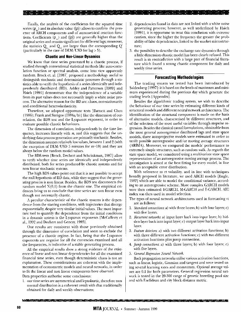
Finally, the analysis of the coefficients for the squared time series (p,) and in absolute value (lpi) allows to confirm the presence of ARCH components and of asymmetrical reaction functions. Coefficients (p,) and ((pi) are generally higher than the original series and remain significant for different lags; moreover, the statistics Q, and Q,*, are larger than the corresponding Q (particularly in the case of DEM/USD for lag > 5).

Chaotic and Non-linear Dynamics We know that time series generated by a chaotic process, if

studied through conventional statistical methods like auto-correlation function or spectral analysis, come into Aew apparently random. Brock et. al. [ 19871 proposed a methodology useful to distinguish stochastic and deterministic processes through a statistics able to verify the hypothesis of a series identically and independently distributed (IID). Ashley and Patterson [1989] and Hsieh [1991] demonstrate that the independence of a variable from its past values does not necessarily imply a white noise process. The alternative reason for the IID are: chaos, non-stationarity and conditional heteroskedasticity.

Therefore, we adopted opportune tests [Barnett and Chen (1986); Frank and Stengos (1988a/b)] like the dimension of correlation, the BDS test and the Lyapunov exponent, in order to evaluate possible chaotic behaliours.

The dimension of correlation, independendy by the time frequency, increases linearly with m, and this suggests that the underlying data process generation are primarily stochastic. Besides, the dimension assumes relatively low\alues, between 1 and 2 (with the exception of DEM/USD 5 minutes for m=lO) and they are always below the random model values.

The BDS tests [Brock, Dechert and Scheinkman, 19871 allow to verify whether time series are identically and independently distributed, both for series produced by chaotic systems and for non linear stochastic systems.

The high BDS values point out that it is not possible to accept the null hypothesis of IID data, while they suggest that the generating process is non linear. Besides, the BDS test disconnects the random model N(O,l) from the chaotic one. The empirical eii- dences bring us to conclude that time series are non linear even though not necessarily chaotic.

A peculiar characteristic of the chaotic systems is the dependence from the starting conditions, with trajectories that diverge exponentially, despite very similar initial values. The most important tool to quantib the dependence from the initial conditions in a dynamic system is the Lyapunov exponents [McCafferty et al., 1992 and Dechert and Gencay, 19931.

Our results are consistent with those previously obtained through the dimension of correlation and seem to exclude the presence of a chaotic regime. In fact, being that the Lyapunol exponents are negative for all the currencies examined and all the frequencies, is indicative of a stable generating process.

All the empirical results show a strong evidence of the existence of linear and non linear dependencies for all the examined financial time series, even though deterministic chaos is not an explanation. These considerations are coherent with the implementation of econometric models and neural networks, in order to fit the linear and non linear components here obsemed. Data properties authorise some conclusions: 1. our time series are asymmetrical and leptokurtic, therefore non

normal distribution is a coherent result with that traditionally obtained for daily and weeklv observations;

2. dependencies found in data are not linked with a white noise generating process; however, as well underlined by Hsieh [ 19911, it is opportune to treat this conclusion with extreme caution, since the higher the frequency the greater the probability of false dependencies, linked to the market microstruc- ture;

3. the possibility to describe the exchange rate dynamics through a little dimension chaotic model has been clearly refused. This result is in contradiction with a large part of financial literature which found a strong chaotic component for daily and weekly time series.

Forecasting Methodologies The trading system we tested has been introduced by

Saidenberg [ 19971: it is based on the levels of maximum and minimum experienced during the prelrious day which generate the trading levels [Appendix].

Besides the algorithmic trading system, we wish to describe the behaliour of our time series by estimating different kinds of structural models and different neural network architectures. The identification of the structural component is made on the basis of alternative models, characterised by different structures, and of the selection of the most useful rariables through stepwise regression. Besides the classical causal formulations, obtainable from the most general autoregressive distributed lags and state space models, three autoprojective models were estimated in order to verify possible autoregressive and/or making ayerage structures (ARIMA). Moreover, we compared the models’ performance to extremely simple structures, such as random walk. As regards the state space model, we considered using a multivariate state space representation of an autoregressire moling average process. The investigation is aimed at the best fitting for every model, in line with an acceptable error distribution.

With reference to rt volatility, and in line with techniques broadly proposed in literature, we used ARCH models [Engle, 19821 which are able to model the conditional variance, according to an autoregressive scheme. More complex GAFXH models were then estimated: I-GARCH, M-GARCH and E-GARCH. AIC index was then used in model selection. The types of neural network architectures used in forecasting rt

are as follows: 1. Standard connections: a) with three layers; b) with four layers; c)

with five layers. 2. Recurrent networlu: a) input layer back into input layer; b) hid-

den layer back into input layer; c) output layer back into input layer.

3. Feature detectors: a) with two different activation functions; b) with three different activation functions; c) with two different actiliation functions plus jump connection.

4. Jump connections: a) with three layers; b) with four layers; c) with five layers.

5. General Regression Neural Network.

Back propagation networks utilise various activation functions, such as linear, logistic, Gaussian and tangent and were tested using several learning rates and momentum. Optimal average values are 0.1 for both parameters. General regression neural network is tested in the 20-300 range of genetic breeding pool size and with Euclidean and city block distance metric.

60 MTA ,JOURNAL * Summer - i\utumn 1999

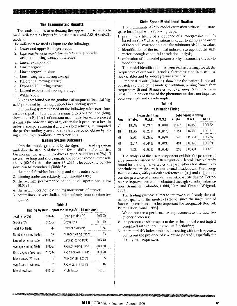
The Econometric Results

The study is aimed at evaluating the opportunity to use technical indicators as inputs into state-space and ARCH-GARCH models. The indicators we used as input are the following:

1. Lower and upper Bollinger Bands 2. Diffuenza fra medie mobili ponderate lineari (Linearly-

weighted maying average difference) 3. Linear extrapolation 4. Linear regression 5. Linear regression slope 6. Linear weighted maying average 7. Differential maying average 8. Exponential maying average 9. Lagged exponential maying average

10. Wilder’s RSI Besides, we found out the goodness of outputs as financial “sig-

nals” produced by the single model in a trading system. Our trading system is based on the following rules: every fore-

cast is a signal and the trader is assumed to take a position (long, short, hold) Pie (-l;tl) of constant magnitude. Forecast is exact if it equals the observed sign of r,, otherwise it produces a loss. In order to compare structural and black box returns, we computed the perfect trading system, i.e. the result we could obtain by taking all the right positions in every period t.

Trading System Outcomes Empirical results generated by the algorithmic trading system

underline the stability of the model for the different frequencies. On ayerage, the system introduces a good reliability (60.7%). If we analvse long and short signals, the former show a lower reliability (50.5%) than the latter (71.2%). The following conclusions can be formulated (Table 3): 1. the model furnishes both long and short indications; 2. winning trades are relatively high (around 60%); 3. the average performance of the single operations is low

(0.0021);

4. the system does not lose the big movements of market; 5. equity lines are very similar, independently from the time fre-

quency.

Table 3

Trading System Report for DEM/USD (10 minutes)

Total net profit 0.0947 Open position P/L 0.0000

Gross profit 0.2087 Gross loss -0.1140

Total # of trades 47 Percent profitable 51%

Number winning trades 24 Number losing trades 23

Largest winning trade 0.0394 Largest-losing trade -0.0240

Average winning trade 0.0087 Average losing trade -0.0050

Ratio avg win/avg loss 1.7544 Avg trade(win & loss) 0.0020

Max consec. Winners 7 Max consec. Losers 5

Avg # bars in winners 71 Avg # bars in losers 46

Max drawdown -0.0457 Profit factor 1.8307

State-Space Model Identification The multivariate ARMA model estimation written in a state-

space form implies the following steps: 1. preliminary fitting of a sequence of autoregressive models

based on Yule-Walker equations in order to identilj the order of the model corresponding to the minimum AIC index value;

2. identification of the technical indicators as input in the state vector through canonical correlation analysis;

3. estimation of the model parameters by maximising the likelihood function. The model identification has been realised testing, for all the

frequencies of our two currencies, alternative models by explica- tive variables and by autoregressive structure.

Empirical results (Table 4) show how the pattern is not ad- equately captured by the models; in addition, passing from higher frequencies (5 and 10 minutes) to lower ones (30 and 60 minutes), the interpretation of the phenomenon does not improve, both in-sample and out-of-sample.

Table 4

Estimation Fitting

In-sample fitting Out-of-sample fitting Freq. N” obs. M.A.E. M.S.E. No obs. M.A.E. M.S.E.

5’ 19,592 0.02178 0.00101 2,177 0.02058 0.00082

10’ 10,362 0.02814 0.00170 1,151 0.02589 0.00131

20’ 5,366 0.03750 0.00294 596 0.03531 0.00236

30’ 3,611 0.04422 0.00433 401 0.03976 0.00329

60’ 1,832 0.06386 0.00848 203 0.05481 0.00667

The analysis of the error component exhibits the presence of an asymmetry associated with a significant leptokurtosis already found for the original variables; the Jarque-Bera test allows us to conclude that we deal with non normal distributions. The Lyung- Box test values, with particular reference to (pyX) and (lpi), point out the presence of a notable heteroskedasttctty degree. Perfor- mance improvement can be obtained through volatility information [Bramante, Colombo, Gabbi, 1998, and Timmer, Weigend, 19971.

The trading purpose allows to improve significantly the estimation quality of the model (Table 5), since the magnitude of forecasting error becomes less important [Dacorogna, Muller, Jost, Pictet, Olsen, Ward, 19961. 1. We do not see a performance improvement as the time fre-

quency decreases; 2. the percentage with respect to the perfect model is not high if

compared with the trading system functioning; 3. the reward-risk index, which is decreasing with the frequency,

points out the presence of risk premia (spread), especially for the highest frequencies.

MTA JOURNAL * Summer - z~utumn 1999 61

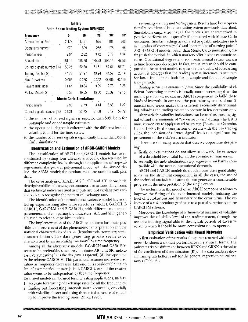
Table 5

State-Space Trading System DEM/USD

Frequency 5' 10' 20' 30' 60

Simulation number 2,177 1,151 596 401 203

Operations number 979 609 266 176 66

Period return 2.94 2.82 3.42 3.79 1.34

Annual return 161.12 138.76 175.78 204.14 48.96

Correct signals number (%) 50.25 52.30 51.51 57.61 57.71

Turning Points (%) 44.73 51.97 40.94 44.57 26.14

Max-Drawdown -0.003 -0.260 -0.342 -0.296 -0.410

Reward Risk Index 11.64 10.84 9.99 12.78 3.28

Perfect Model (%) 6.59 19.55 16.50 23.32 12.15

Monte Carlo Simulations

Period return 2.90 2.79 3.44 3.83 1.32

Correct signals number (%) 51.31 52.75 51.68 57.9 57.72

1. the number of correct signals is superior than 50%, both for in-sample and out-of-sample estimates;

2. the operational degree is coherent with the different level of volatility found for the time series;

3. the number of current signals is significantly higher than Monte Carlo simulations.

Identification and Estimation of ARCH-GARCH Models The identification of ARCH and GARCH models has been

conducted bp testing four alternative models, characterised b) different complexity levels, through the application of stepwise regressions: the general polynomial model with distributed de- lays; the ARMA model; the random walk; the random walk plus drift.

The error analysis of MAE., M.S.E., SIC and =UC, shows little descriptive ability of the single econometric structures. This means that technical indicators used as inputs are not explanatory variables able to recognise the pattern of exchange rate.

The identification of the conditional variance model has been led up experimenting alternative structures (ARCH, GARCH, I- GARCH, GARCH-M and E-GARCH), with different number of parameters, and comparing the indicators (AIC and SIC) generally used to select competitive models.

The implementation of the ARCH component has made possible an improvement of the phenomenon interpretation and the statistical characteristics of errors (leptokurtosis, symmetry, serial autocorrelation). The data generating process seems to be characterised by an increasing “memory” by time frequency.

Among all the alternative models, E-GARCH and GARCH-M seem to be preferable, since they minimise XC and SIC indicators. Ve? meaningful is the risk premia (spread) (d) incorporated in the scheme GARCH-M. This parameter assumes more elevated values as frequency decreases. Likewise, it is considerable the effect of asymmetrical answer (u in E-GARCH), even if the relative value seems to be independent by the time frequency. Estimated models can be used for interesting applications, such as: 1. accurate forecasting of exchange rates for all the frequencies; 2. finding out forecasting intervals more accurately, especially

with volatility cluster and using theoretical measure of volatility to improve the trading rules [Zhou, 19961.

Forecasting accurat7; and tradingsytem. Results have been opera- tionally experienced-into the trading system previously described. Simulations emphasize that all the models are characterised b! positive performance, especially if compared with Monte Carlo outcomes. Similar findings are offered by quality indicators such as ‘number of correct signals” and “percentage of turning point.” ARCH-GARCH models, better than hlonte Carlo simulations, distinguish the periods in which markets offer higher economic returns. Operational degree and economic annual return worsen as time frequency decreases. In fact, annual return should be compared to the perfect model, to quantify the quality of forecasting activity it emerges that the trading system increases its accurac!- for lower frequencies, both for in-sample and for out-of-sample time periods.

T,ading sytem and operationalfilters. Since the availability of efficient forecasting intervals is usually more interesting than the instant prediction, we can use ARCH component to build these kinds of intervals. In our case, the particular drnamics of our financial time series makes this criterion excessively discriminat- ing, allowing the trading system to operate in few occasions only.

,%lternatively, volatility indications can be used as tracking signal to find the moments of “excessive noise,” during which it is more convenient to apply a stand-by strategy [Bramante, Colombo, Gabbi, 19981. By the comparison of results with the two trading rules, the inclusion of a “trace signal” leads to a significant improvement of the risk/return indicator.

There are still many aspects that deseme opportune deepen- ing: a. firstly, our estimations do not allow us to verify the existence

of a threshold level valid for all the considered time series; b. secondly, the individualisation step requires terms hardly com-

patible with the normal operational demands. ARCH and GARCH models do not demonstrate a good ability

to define the structural component; in all the cases, the use of the technical analysis indicators do not generate a considerable progress in the interpretation of the single events.

The inclusion in the model of an ARCH component allows to improve the fitting of the experimented models, reducing the level of leptokurtosis and a.s!;mmetry of the error terms. The existence of a risk premium guides us to a partial superiority of the GARCH-M scheme.

Moreover, the knowledge of a theoretical measure of volatility improves the reliability level of the trading system, through the use of a tracking signal able to distinguish periods of excessive volatility when it should be more convenient not to operate.

Empirical Verification with Neural Networks A first evaluation of the results altogether reached with neural

networks shows a modest performance in statistical terms. The only remarkable difference between BPSN and GRNN is the value of the coefficient of determination (R’). The data analyses show a meaningfully better result for the general regression neural networks (Table 6).

MTA JOURNAL 0 Summer - .Autumn 1999

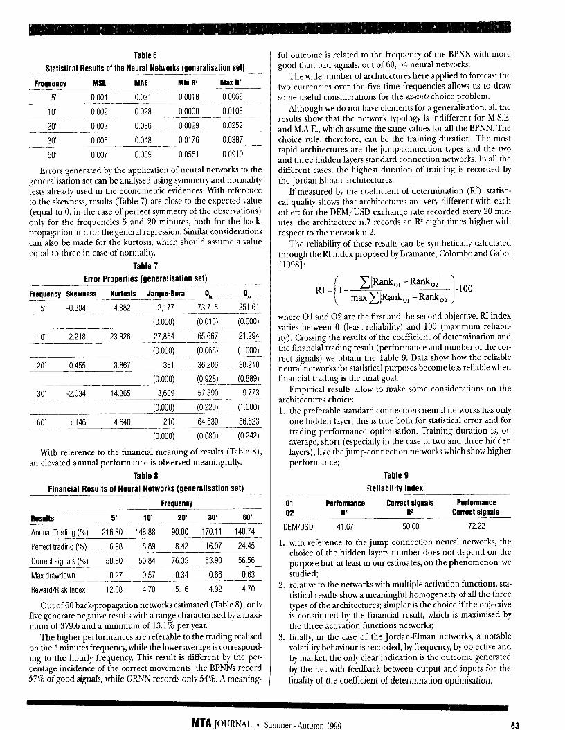
Table 6

Statistical Results of the Neural Networks (generalisation set)

Frequency MSE MAE Min R2 Max II2

5’ 0.001 0.021 0.0018 0.0069

10’ 0.002 0.028 0.0000 0.0103

20’ 0.002 0.036 0.0029 0.0252

30’ 0.005 0.048 0.0176 0.0387

60’ 0.007 0.059 0.0561 0.0910

Errors generated by the application of neural networks to the generalisation set can be analysed using symmetry and normality tests already used in the econometric evidences. With reference to the skewness, results (Table 7) are close to the expected value (equal to 0, in the case of perfect symmetry of the observations) only for the frequencies 5 and 20 minutes, both for the back- propagation and for the general regression. Similar considerations can also be made for the kurtosis, which should assume a value equal to three in case of normality.

Table 7

Error Properties (generalisation set) - Frequency Skewness Kurtosis Jarque-Bera 0, h-

5’ -0.304 4.882 2,177 73.715 251.61 -- (0.000) (0.016) (0.000)

10’ -2.218 23.826 27,864 65.667 21.294

(0.000) (0.068) (1.000)

20’ 0.455 3.867 381 36.206 38.210

(0.000) (0.928) (0.889)

30’ -2.034 14.365 3,609 57.390 9.773

(0.000) (0.220) (1.000)

60’ 1.146 4.640 210 64.630 56.623

(0.000) (0.080) (0.242)

With reference to the financial meaning of results (Table 8)) an elevated annual performance is observed meaningfully.

Table 8

Financial Results of Neural Networks (generalisation set) - Frequency

RlSUltS 5’ 10’ 20’ 30 50’

Annual Trading (%) 216.30 148.88 90.00 170.11 140.74

Perfect trading (%) 6.98 8.89 8.42 16.97 24.45

Correct signals (%) 50.80 50.84 76.35 53.90 56.56

Max drawdown 0.27 0.57 0.34 0.66 0.63

Reward/Risk Index 12.08 4.70 5.16 4.92 4.70

Out of 60 back-propagation networks estimated (Table 8)) only five generate negative results with a range characterised by a maximum of 379.6 and a minimum of 13.1% per year.

The higher performances are referable to the trading realised on the 5 minutes frequency, while the lower average is corresponding to the hourly frequency. This result is different by the percentage incidence of the correct movements: the BPNNs record 57% of good signals, while GRNN records only 54%. A meaning-

ful outcome is related to the frequency of the BPNN with more good than bad signals: out of 60,54 neural networks.

The wide number of architectures here applied to forecast the two currencies over the five time frequencies allows us to draw some useful considerations for the ex-ante choice problem.

Although we do not have elements for a generalisation, all the results show that the network typology is indifferent for M.S.E. and MAE., which assume the same values for all the BPNN. The choice rule, therefore, can be the training duration. The most rapid architectures are the jump-connection types and the two and three hidden layers standard connection networks. In all the different cases, the highest duration of training is recorded by the Jordan-Elman architectures.

If measured by the coefficient of determination (R2), statistical quality shows that architectures are very different with each other: for the DEM/USD exchange rate recorded every 20 minutes, the architecture n.7 records an R* eight times higher with respect to the network n.2.

The reliability of these results can be synthetically calculated through the RI index proposed by Bramante, Colombo and Gabbi [1998]:

where 01 and 02 are the first and the second objective. RI index varies between 0 (least reliability) and 100 (maximum reliability). Crossing the results of the coefficient of determination and the financial trading result (performance and number of the correct signals) we obtain the Table 9. Data show how the reliable neural networks for statistical purposes become less reliable when financial trading is the final goal.

Empirical results allow to make some considerations on the architectures choice: 1. the preferable standard connections neural networks has only

one hidden layer; this is true both for statistical error and for trading performance optimisation. Training duration is, on average, short (especially in the case of two and three hidden layers), like the jump-connection networks which show higher performance;

Table 9

Reliability Index

01 Performance Correct signals Performance 02 II2 II2 Correct signals

DEMIUSD 41.67 50.00 72.22

1. with reference to the jump connection neural networks, the choice of the hidden layers number does not depend on the purpose but, at least in our estimates, on the phenomenon we studied;

2. relative to the networks with multiple activation functions, statistical results show a meaningful homogeneity of all the three types of the architectures; simpler is the choice if the objective is constituted by the financial result, which is maximised by the three activation functions networks;

3. finally, in the case of the Jordan-Elman networks, a notable volatility behaviour is recorded, by frequency, by objective and by market; the only clear indication is the outcome generated by the net with feedback between output and inputs for the finality of the coefficient of determination optimisation.

MTA JOCRhN * Summer - Autumn 1999 63

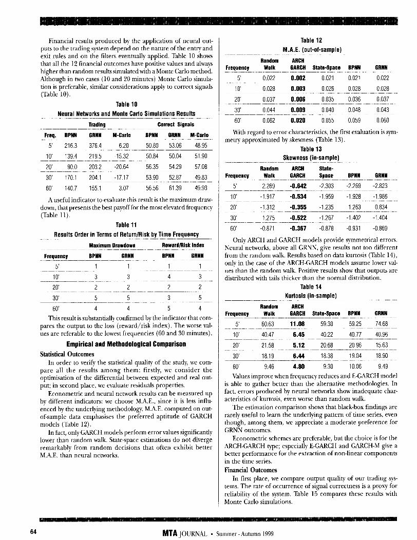
Financial results produced by the application of neural outputs to the trading system depend on the nature of the entry and exit rules and on the filters eventually applied. Table 10 shows that all the 12 financial outcomes have positive values and always higher than random results simulated with a Monte Carlo method. Although in two cases (10 and 20 minutes) Monte Carlo simulation is preferable, similar considerations apply to correct signals (Table 10).

Table 10

Neural Networks and Monte Carlo Simulations Results

Trading Correct Signals

Freq. BPNN GRNN M-Carlo BPNN GRNN M-Carlo

5’ 216.3 376.4 6.20 50.80 53.06 48.95

10' 139.4 219.5 -15.32 50.84 50.04 51.90

20' 90.0 203.2 -20.64 56.35 54.29 57.08

30' 170.1 204.1 -17.17 53.90 52.87 49.83

60' 140.7 155.1 3.07 56.56 61.39 49.93

A useful indicator to evaluate this result is the maximum drawdown, that presents the best payoff for the most elevated frequency (Table 11).

Table 11

Results Order in Terms of Return/Risk by Time Frequency

Maximum llrawdown Reward/Risk index

Frequency BPNN GRNN BPNN GRNN I__--

5' 1 1 1 1

10' 3 3 4 3 __-- 20' 2 2 2 2

30' 5 5 3 5

60' 4 4 5 4

This result is substantially confirmed by the indicator that compares the output to the loss (reward/risk index). The worse values are referable to the lowest frequencies (60 and 30 minutes).

Empirical and Methodological Comparison

Statistical Outcomes In order to verify the statistical quality of the study, we com-

pare all the results among them: firstly, we consider the optimisation of the differential between expected and real output; in second place, we evaluate residuals properties.

Econometric and neural network results can be measured up by different indicators: we choose M.A.E., since it is less influ- enced by the underlying methodology. M.A.E. computed on out- of-sample data emphasises the preferred aptitude of GARCH models (Table 12).

In fact, only GARCH models perform error values significantly lower than random walk. State-space estimations do not diverge remarkably from random decisions that often exhibit better M.A.E. than neural networks.

Table 12

M.A.E. (out-of-sample)

Random ARCH Frequency Walk GARCH State-Space BPNN GRNN

5' 0.022 0.002 0.021 0.021 0.022

10' 0.028 0.003 0.026 0.028 0.028

20' 0.037 0.006 0.035 0.036 0.037

30' 0.044 0.009 0.040 0.048 0.043

60' 0.062 0.020 0.055 0.059 0.060

With regard to error characteristics, the first evaluation is symmetry approximated by skewness (Table 13).

Table 13 Skewness (in-sample)

Random ARCH State- Frequency Walk GARCH Space BPNN GRNN

5' -2.269 -0.642 -2.303 -2.269 -2.823

10' -1.917 -0.534 -1.959 -1.928 -1.986 --

20' -1.312 -0.355 -1.235 -1.263 -0.834 ._____

30' -1.275 -0.522 -1.267 -1.402 -1.404

60' -0.871 -0.367 -0.878 -0.931 -0.869

Only ARCH and GARCH models provide symmetrical errors. Neural networks, above all GRNN, give results not too different from the random walk. Results based on data kurtosis (Table 14)) only in the case of the ARCH-GARCH models assume lower values than the random walk. Positive results show that outputs are distributed with tails thicker than the normal distribution.

Table 14 Kurtosis (in-sample)

Random ARCH Frequency Walk GARCH State-Space BPNN GRNN ~______

5' 60.63 11.06 59.30 59.25 74.68

10' 40.47 6.45 40.22 40.77 40.96

20' 21.58 5.12 20.68 20.96 15.63

30' 18.19 6.44 18.38 19.04 18.90

60' 9.46 4.80 9.30 10.06 9.49

Values improve when frequency reduces and E-GARCH model is able to gather better than the alternative methodologies. In fact, errors produced by neural networks show inadequate characteristics of kurtosis, even worse than random walk.

The estimation comparison shows that black-box findings are rarely useful to learn the underlying pattern of time series, even though, among them, we appreciate a moderate preference for GRNN outcomes.

Econometric schemes are preferable, but the choice is for the ARCH-GARCH type; especially E-GARCH and GARCH-M give a better performance for the extraction of non-linear components in the time series. Fiicial Outcomes

In first place, we compare output quality of our trading systems. The rate of occurrence of signal correctness is a proxy for reliability of the system. Table 15 compares these results with Monte Carlo simulations.

64 MTA JOURNAL l Summer -Autumn 19%

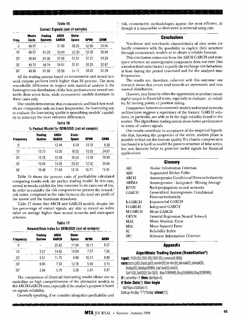
Table 15

Correct Signals (out-of-sample) ..--- - - Monte Trading ARCH State-

Freq. Carlo Systems GARCH Space BPNN GRNN -- ______-

5’ 48.97 - 51.99 50.25 52.66 53.06

ii' 49.57 61.29 53.64 52.30 52.26 50.04

20' 49.84 61.96 52.06 51.51 57.31 54.29

30' 49.75 58.24 54.81 57.61 55.25 52.87

60' 49.99 61.80 55.56 57.71 58.42 61.39

All the trading systems based on econometric and neural network outputs perform levels higher than 50 percent. The most remarkable difference in respect with statistical analysis is the heterogeneous distribution of the best performances: neural networks show seven bests, while econometric models dominate in three cases only.

Our results demonstrate that econometric and black box models are competitive only on lower frequencies. An interesting way to evaluate the forecasting quality is quantifying models’ capabil- ity to intercept the most extensive differences.

Table 16

% Perfect Model for DEMNSD (out-of-sample)

Trading ARCH State- Frequency System GARCH Space BPNN GRNN

5' 12.44 6.59 10.75 a.38

10' 13.23 12.20 19.55 10.55 24.87

20' 13.78 15.49 16.50 13.39 20.99

30' 19.04 14.25 23.32 12.32 29.66

60' la.48 21.64 12.15 18.71 15.45

Table 16 shows the percent ratio of profitability calculated comparing results with the perfect trading model. In this case, neural networks exhibit the best outcome in six cases out of ten. In order to consider the risk component we present the reward/ risk index, computed as the ratio between the total net profit of the system and the maximum drawdown.

Table 17 shows that ARCH and GARCH models, despite the low percentage of correct signals, are able to record an index value on average higher than neural networks and state-space schemes.

Table 17

Reward/Risk Index for DEM/USD (out-of-sample)

Trading ARCH State- Frequency System GARCH Space BPNN GRNN

5' 25.82 11.64 18.11 a.27

10' 3.57 14.45 10.84 7.37 7.92

20' 3.51 11.75 9.99 10.31 a.89

30' 9.06 7.33 12.78 5.90 9.13

60' 3.04 5.76 3.28 5.41 8.87

The comparison of financial forecasting results allows one to underline an high competitiveness of the alternative models to the ARCH-GARCH ones, especially if the analyst’s purpose is based on signals reliability.

Generally speaking, if we consider altogether profitability and

risk, econometric methodologies appear the most efficient, although it is impossible to determine a universal using rule.

Conclusions Non-linear and not-chaotic characteristics of time series are

hardly consistent with the possibility to explicit their structure through econometric models so to obtain a reliable forecast.

This conclusion comes out from the ARCH-GARCH and state- space schemes: an autoregressive component does not exist (but a modest third order factor) tojustify the exchange rate behaviour, at least during the period examined and for the analysed time frequencies.

The results are, therefore, coherent with this outcome: our research shows that errors tend towards an asymmetric and non normal distribution.

However, non linearity offers the opportunity to produce meaningful output in financial terms, especially to evaluate: a) volatility; b) turning points; c) position taking.

Comparison between econometric models and neural networks architectures suggests a supremacy of the former: GARCH solu- tions, in particular, are able to fit the high volatility found in the market. The algorithmic trading system shows better performance in terms of correct signals.

Our results contribute to acceptance of the empirical hypothesis that, knowing the properties of the series, analysis phase is possible to find out the forecast quality. If a chaotic component is not found it is hard to model the pattern structure of time series, but non linearity helps to generate useful signals for financial applications.

Glossary AIC Akaike Information Criterion ADF Augmented Dickey Fuller ARCH Autoregressive Conditional Heteroschedasticity ARM4 Autoregressive - Integrated - Moving Average BPNN Back-propagation neural networks GARCH Generalized Autoregressive Conditional

Heteroschedasticity E-GARCH Exponential GARCH I-GARCH Integrated GARCH M-GARCH Mean GARCH GRTVN General Regression Neural Network

Mean Absolute Error MSE Mean Squared Error RI Reliability Index SIC Schwarze Information Criterion

Appendix

Algorithmic Trading System (TradeStation@) input: fl(O.05),f2(0.35),f3(0.55),reverse(0.006); vars:ssetup(O),bsetup(O),senter(O),benter(O),bbreak(O),sbreak(O),

Itoday(O),htoday(9999),startsys(O),div(O), Selll(O),Sell2(0),Sell3(0), Buy1(99999),Buy2(99999),Buy3(99999);

if currentbar=l then startsys=O; if DateAtate[l I then begin startsys=startsystl ;

bsetup=ltoday-fl*(htoday-close[ll);

MTA JOURNAL * Summer - &rtumn 1999 65

ssetup=htodaytfl *(close[l I-ltoday); senter=((ltf2)/2)*(htodaytclose[ll)-(f2)*ltoday; benter=((l -tf2)/2)*(ltodaytclose[ll)-(f2)*htoday; bbreak=ssetuptf3*(ssetup-bsetup); sbreak=bsetup-f3*(ssetup-bsetup); htoday=h;ltoday=l;

end; if high>htoday then htoday=high; if low<ltoday then Itoday=low; Selll=O;Sell2=O;Sell3=0; Buyl=99999;Buy2=99999;Buy3=99999; if startsys>=2 and Date>entrydate(l) then begin

if marketposition=-l then Buyl=entryprice-treverse; {BUY LEVEL STOP AND REVERSE) if marketposition= 1 then Selll=entryprice-reverse; {SELL LEVEL STOP AND REVERSE)

(BUY REVERSAL LEVEL) if Itodayc=bsetup and marketpositiono 1 then Buy2=benter-(bsetup- Itoday)/3;

(SELL REVERSAL LEVEL1 if htoday>=ssetup and marketpositiono-l then Sell2=sentert(htoday- ssetup)/3; if marketposition=O then BuyS=bbreak; {BREAKOUT BUY LEVEL1 if marketposition=O then Sell3=sbreak; {BREAKOUT SELL LEVEL]

end; IF (Selll>=Sell2 AND Selll>=Sell3) THEN SELL at Sell1 stop ELSE IF Sell2>=Sell3 THEN SELL at Sell2 stop ELSE SELL at Sell3 stop; IF (Buyl<=Buy2 AND Buyl<=BuyS) THEN BUY at Buy1 stop ELSE IF Buy2<=Buy3 THEN BUY at Buy2 stop ELSE BUY at Buy3 stop;

References Ashley R.A., Patterson D.M., 1989, Linear uersus NonlinearMac- roeconomics: A Statistical Test International Economic Review, 30 (3)) 685-704. Bamett W., Chen, P., 1986, The Aggregation-Theoretic Monetary Aggregates are Chaotic and Haue Strange Attractions, in W. Barnett, E. Bemdt and H. R White (eds), Dynamic Econometric Mod- elling. Cambridge: Cambridge University Press.

q Bramante R., Colombo R., Gabbi G., 1998, Are Neural Network and Econometric Forecasts Good for Trading? Stochastic Variance MO&~ as a Filter Rule, in A.-P. N. Refenes - A. N. Burgess -J. E. Moody (eds), Decision Technologies for Computational Man- agement Science, Kluwer Academic Publishers, Boston.

m Brock W.A., Dechert W.D., Scheinkman J.A., 1987, A Test for Independence Based on the Correlation Dimension, Working Paper, University of Houston and University of Chicago. Dacorogna M.M., Muller U.A., Jost C., Pictet O.V., Olsen R.B., Ward J.R., 1996, Heterogeneous Real-time Trading Strategies in the Fn-eign Exchange Market, in C. Dunis (eds.) Forecasting Finan- cial Markets, John Wiley, New York.

IB Dechert W.D., Gencay R., 1993, Lyapunov Exponents as a Non- parametric Diagnostic for Stability Analysis, Journal of Applied Econometrics, 7, S41-S61. Diebold F.X., 1988, Lecture Notes in Economics and Mathematical System, Springer-Verlag, New York.

RI Engle R.F., 1982, Autoregressive Conditional Heteroskedasticity with

Estimates of the Variance of United Kingdom Inflation, Econometrica, 50, 987-1008. Frank M.Z., Stengos T., 1988a, ChaoticQnamics in Economic Time Series, Journal of Economic Surveys 2,103133. Frank M.Z. Stengos T., 1988b, Some Evidence Concerning Macro- economic Chaos, Journal of Monetary Economics 22, 423-438.

m Hsieh D. A., 1991, Chaos and NonlinearL+amics: Application to Financial Market, The Journal of Finance, No.5. McCafferty D.F., Ellner S. Gallant A.R., Nychka D.W., 1992, Estimating the Lyapunov Exponent of a Chaotic System with Non- parametric Regression, Journal of American Statistical Associa- tion, 87. Muller U.A., Dacorogna M.M., Embrechts P., Samorodnitsky G., 1995, How Heavy are the Tails of a Stationary HARCH Process? A Study of the Moments, Internal document O&A Research Group. Saidenberg R., 1997, Trading with a 100% Mechanical Approach, Workshop Proceedings, Milan.

q Timmer J., Weigend A.S., 1997, Modelling Volatility Using State Space Models, in International Journal of Neural Systems, Vol. 8, No. 5. Zhang G., Patuwo B. E., Hu M. Y, 1998, Forecasting with Artiji- cial Neural Networks: The State of the Art, International Journal of Forecasting, vol. 14. Zhou B., 1996, Forecasting Foreign Exchange Rates Subject to De- volatilization, in C. Dunis (ed), Forecasting Financial Markets -Exchange Rates, Interest Rates and Assets Management, John Wiley & Sons, Chickester, England.

Giampaolo Gabbi

The Authors

Graduated in Economics at University of Parma, Ph.D. in Financial Economics at Bocconi University Milan, Associate Professor of Banking and Management Department, Univer- sity of Siena, Italy and in the Credit Area, SDA Bocconi, Milan

Ruggero Colombo Graduated in Economics at Catholic University of Milan, Pro- fessor of Statistics at Institute of Statistics, Catholic Univer- sity, Milan

Riccardo Bramante Graduated in Economics at Catholic University of Milan, Pro- fessor of Statistics at Institute of Statistics, Catholic Univer- sity, Milan

Maria Paola Viola Graduated in Economics at Catholic University of Milan, Risk Manager at RAS, Milan

Paolo De Vito Graduated in Information Technology at University of Turin, CEO of IT Trading, Turin

Albert0 Tumietto Graduated in Economics at Bocconi University, Milan; Pri- vate Banking Manager at Banca Nazionale dell’Agricoltura, Milan; President of SIAT, Italian Technical Analysts Associa- tion

66 MTA JOURhNL * Summer -Autumn 1999

journal of technical analysis (jota). issue 52 (1999, summer)

Economy & Finance

cmt kirkpatrick

cmt dorsey

cmt teladvisor

cmt aerodynamicinvestmentsinc

cfa john

mta journal staff summer

cmt ustsecurities princeton

cmt lake quivira