Journal of Computational Physics 231 (2012) 4836–4847

Contents lists available at SciVerse ScienceDirect

Journal of Computational Physics

journal homepage: www.elsevier .com/locate / jcp

Fast iterative interior eigensolver for millions of atoms

Gerald Jordan ⇑, Martijn Marsman, Yoon-Suk Kim, Georg KresseUniversity of Vienna, Faculty of Physics, Department for Computational Materials Physics, Vienna, Austria

a r t i c l e i n f o

Article history:Received 28 July 2011Received in revised form 29 March 2012Accepted 2 April 2012Available online 17 April 2012

Keywords:Electronic structure calculationsDavidson methodHarmonic Ritz valuesInterior eigenvalue problem

0021-9991/$ - see front matter � 2012 Elsevier Inchttp://dx.doi.org/10.1016/j.jcp.2012.04.010

⇑ Corresponding author.E-mail address: gerald.jordan@univie.ac.at (G. Jo

a b s t r a c t

We show that a combination of the Generalized Davidson method and harmonic Ritz val-ues (called harmonic Davidson) is well-suited for solving large interior eigenvalue prob-lems using a plane wave basis. The algorithm enables us to calculate impurity and bandedge states for systems of 100,000 atoms in about one day on 32 cores. We demonstratethe capabilities of the method by calculating the electronic states of a large GaAs quantumdot embedded in an AlAs matrix.

� 2012 Elsevier Inc. All rights reserved.

1. Introduction

Electronic structure calculations on large systems face a computational bottleneck because conventional methods scalewith the third power of the system size. In these calculations, one determines all N occupied eigenstates of a given single-particle Hamiltonian. Cubic scaling is then a consequence of keeping the N eigenvectors of size / N orthogonal to eachother. There are two principal methods to overcome the scaling problem. (i) The most common approach assumes rapiddecay of the density matrix, which allows to truncate the density matrix at some finite distance resulting in linear scalingwith system size [1]. Linear scaling electronic structure methods have been implemented in many density functional the-ory codes such as CONQUEST [2,3], SIESTA [4], and ONETEP [5]. Although calculations for up to millions of atoms havebeen demonstrated to be feasible with such codes [6] calculations for more than 10,000 atoms are very time consuming.(ii) For many applications, however, it is sufficient to determine a few selected eigenstates in the interior of the spectrum.For instance, the electronic and optical properties of semiconductor nanostructures are often mainly determined by statesclose to the valence and conduction band edges. This approach has been pioneered by the group of Wang and Zunger [7–9] and is nowadays easily applicable to a million atoms, although it has the drawback that it needs to be combined withsuitable semi-empirical pseudopotentials, since the traditional density functional theory self-consistency cycle is notapplicable. In this work we will concentrate on this approach, specifically on the efficient numerical calculation of selectedstates close to the valence and conduction band edges. Although calculating only selected states reduces the computa-tional effort in principle, the associated interior eigenproblem turns out to be much more difficult to cope with numeri-cally than the now almost routine task of finding the smallest eigenvalues and corresponding eigenvectors of a givenHamiltonian matrix H.

In the interior eigenproblem, one searches for eigenpairs, i.e. eigenvectors /a and associated eigenvalues �a,

Hj/ai ¼ �aj/ai; ð1Þ

. All rights reserved.

rdan).

G. Jordan et al. / Journal of Computational Physics 231 (2012) 4836–4847 4837

with �a close to some reference energy �ref in the interior of the spectrum of H. The band index a takes on values from 1 to Nb,the number of bands included in the calculation. Non-norm conserving pseudopotentials are often used to reduce the size ofthe plane wave basis [10–12]. This leads to a generalized eigenproblem

Hj/ai ¼ �aSj/ai; ð2Þ

with the overlap matrix S.In large-scale ab-initio calculations, H is of a size that prevents it from ever being formed and stored explicitly. Further-

more, for a plane wave basis set, the matrix–vector product Hj/i can be evaluated in O(N logN) operations (N being the size ofthe plane wave basis set) using fast Fourier transforms (FFTs), much faster than by straightforward matrix–vector multipli-cation, which requires O(N2) operations. For these reasons, one is practically limited to iterative subspace methods, which –in one way or another – construct a subspace V. V is usually of the Krylov type KnðA;/Þ ¼ spanfj/i;Aj/i; . . . ; An�1j/ig, whicharises from repeated application of an operator A onto a vector /. In the very simplest case, A is chosen to be H, but in generalthis is modified because of the presence of the overlap matrix S and the use of preconditioners K. From the subspace V, oneextracts an approximation to the eigenvalues and eigenvectors that are optimal in some specified sense. This is commonlydone by calculating the Ritz vectors and values, i.e. by solving the eigenproblem within the subspace V (see next section). Ifone seeks the eigenvector whose eigenvalue is closest to some reference energy �ref, one faces the problem of selecting thebest approximating Ritz vector.

It is known that the extremal Ritz values are usually meaningful approximations to exterior eigenvalues, and the associ-ated Ritz vectors can be expected to have significant overlap with the corresponding eigenvectors [13,14]. For Ritz values inthe interior of the spectrum, the relationship between the Ritz vectors and true eigenvectors with nearby eigenvalues is lessclear. In general, the interior Ritz values do not qualify as useful approximations for the interior eigenvalues because theymay result from averaging over larger and smaller eigenvalues than desired by �ref. Thus the associated Ritz vector may actu-ally contain only a small contribution from eigenvectors whose eigenvalues are closest to the Ritz value.

The issue is particularly problematic when one restarts the Krylov space iteration, since when restarting from an unsuit-able vector one loses all information acquired so far. Restarts are usually unavoidable because, as the dimension of the Krylovsubspace increases, the memory requirements and the Ritz diagonalization will eventually become too expensive. To cir-cumvent this problem, one strives to map the desired interior eigenvalues to extremal ones by means of a spectraltransformation.

One such method that has been successfully applied to electronic structure problems is the ‘‘folded spectrum method’’developed by Wang and Zunger [15]. Here the transformation consists in squaring the shifted Hamiltonian, i.e. solving

ðH � �ref Þ2j/ai ¼ ð�a � �ref Þ2j/ai; ð3Þ

such that the original eigenvalues closest to �ref are mapped onto the smallest eigenvalues of the folded operator. However,squaring the Hamiltonian also squares the condition number of the problem, degrading the overall convergence rate. More-over, extending the folded spectrum method to generalized eigenproblems leads to [16]

ðH � �ref SÞS�1ðH � �ref SÞj/ai ¼ ð�a � �ref Þ2Sj/ai; ð4Þ

which further aggravates the difficulty of the problem, since it requires solving linear equations with the overlap matrix S. AsS has the same dimension as H and cannot be inverted straightforwardly, this would in practice imply a second inner iter-ation process.

Another suitable and well-known spectral transformation is shift-and-invert [17]

ðH � �ref SÞ�1Sj/ai ¼1

�a � �refj/ai; ð5Þ

which maps the eigenvalues closest to �ref to the lowest or highest part of the transformed spectrum. However, this againrequires the costly solution of linear systems with H � �refS at each step.

2. The algorithm

It turns out that one can benefit from the shift-and-invert transformation without ever solving a linear system via the so-called harmonic Ritz values. While first applied to interior eigenproblems already in [18], the harmonic Ritz values were for-mally introduced under this term and theoretically investigated in [19].

For practical applications, harmonic Ritz values have been combined with different ways of constructing the search sub-space. The Jacobi–Davidson algorithm [20,21] solves the Jacobi correction equation for this purpose. This scheme was usedfor electronic structure problems in [16], but it was applied to small- and medium-size systems only. The conventionalDavidson approach for constructing the subspace leads to the harmonic Davidson method introduced in [14], which has beenapplied to calculation of excited states in molecules of medium size [22].

We implemented the harmonic Davidson method in VASP, the Vienna ab-initio Simulation Package [23] and demonstratethe successful application of this method to very large systems of up to 100,000 atoms. Our algorithm handles generalized

4838 G. Jordan et al. / Journal of Computational Physics 231 (2012) 4836–4847

eigenvalue problems and avoids the iterative solution of an inner linear problem, and it is significantly simpler to implementthan the one suggested in [16].

As mentioned above, iterative eigensolvers seek the best approximation to the eigenpairs within some search subspaceand basically comprise two steps: 1. subspace extraction, and 2. subspace expansion. We will consider these two steps of ouralgorithm separately.

We first describe the optimization of a single band and afterwards point out the differences in the blocked version, whereseveral bands are optimized simultaneously.

2.1. Subspace extraction – harmonic Ritz values

Given a search subspace Vk ¼ rangeðVkÞ, with Vk = [jv1i, jv2i, . . . , jvki] (abbreviated by V), we want to extract a linear com-bination jvai ¼

Pkj¼1ca;jjv ji ¼ Vca and a scalar ha that best approximate the eigenvector j/ai and the corresponding eigen-

value �a,

jvai � j/ai; ha � �a: ð6Þ

One possibility to do this is to minimize the residual [24,25]. Another possibility is to introduce a second subspace, the testsubspace Wk ¼ rangeðWkÞ; Wk ¼ ½jw1i; jw2i; � � � ; jwki� (abbreviated by W), and impose a condition of Galerkin type, i.e. de-mand that the eigenvalue equation be orthogonal to W. This projects the original high-dimensional eigenproblem onto alower-dimensional one.

Following [16], we define the shifted eigenproblem,

eHj/ai ¼ ~�aSj/ai ð7Þ

with eH ¼ H � �ref S and ~�a ¼ �a � �ref , and the corresponding approximate eigenvalue eha � ~�a.In most methods, one takes W = V (the so-called orthogonal projection method [26]) and solves

V y eHVca ¼ ehaV ySVca ð8Þ

to calculate the Ritz values eha and Ritz vectors jvai = Vca in the search subspace.Choosing V and W differently leads to an oblique projection method [26]. In particular, setting W ¼ eHV , we arrive at har-

monic Ritz values. The resulting equation is

Wy eHVca ¼ ehaWySVca: ð9Þ

By the simple replacement V ¼ eH�1W , one sees that this equation is actually equivalent to

WySeH�1Wca ¼1eha

WyWca; ð10Þ

i.e. to an orthogonal projection of the shift-inverted problem (see Eq. (5)). The approximate eigenvalues eha obtained from Eq.(9) are called harmonic Ritz values. Since the original eigenvalues �a closest to �ref correspond to the eha closest to zero andthus to extremal Ritz values 1=eha of Eq. (10), we expect the harmonic formulation to provide good approximations preciselyfor them. Hence the vector jvai with smallest jehaj is chosen as the optimal solution for this subspace.

Note, however, that in contrast to Eq. (8), the projection subspace of Eq. (10) is not the (Krylov-like) subspace built withthe shift-inverted operator SeH�1, but still the space associated with eH.

Furthermore, we point out that the obliquely projected generalized eigenproblems in Eqs. (9) and (10) involve thenon-hermitian matrices W�S V and WySeH�1W , respectively. Thus, they may, and in practice do, have complex eigenvalues– notwithstanding that the underlying unprojected problem Eq. (7) is hermitian. If we encounter complex eigenvalues inour calculation, we replace them by their absolute value. This causes no difficulty since the converged solutions correspondto real eigenvalues anyway.

2.2. Subspace expansion – Generalized Davidson, orthogonalization

The subspace extraction provides a candidate eigenpair (jvai,ha) from the search subspace Vk. After that, the question ishow to expand the set Vk ´ Vk+1 = [Vk, jvk+1i] to increase the subspace such that the solution improves.

To assess the error in the approximate solution and find corrections to it, an important quantity is the residual vector

jrai :¼ ðH � qaSÞjvai; ð11Þ

where

qa :¼ hvajHjvaihvajSjvai

ð12Þ

is the Rayleigh quotient of jvai.

G. Jordan et al. / Journal of Computational Physics 231 (2012) 4836–4847 4839

The Jacobi–Davidson method obtains the expansion vector jvk+1i by solving a linear system. This is prohibitively expen-sive for the huge and dense matrices that arise in our plane wave code. Instead, we found that a conventional GeneralizedDavidson (GD) approach leads to fast and stable convergence.

In the GD method, the search space is expanded by

jvkþ1i � Kjrai; ð13Þ

where K is a preconditioner approximating the inverse of H � �aS. In the original Davidson prescription, K was chosen as theinverse of the diagonal of H � qaI. In our algorithm, we adopted the preconditioning function proposed by Teter et al. [27],

K ¼X

q

2jqihqj32 Ekin

27þ 18xþ 12x2 þ 8x3

27þ 18xþ 12x2 þ 8x3 þ 16x4 with x ¼ �h2

2me

q2

32 Ekin

; ð14Þ

Ekin ¼X

q

�h2q2

2mehv1jqihqjv1i; ð15Þ

where q runs over all plane waves included in the basis set. Ekin is the kinetic energy of the electronic state and is calculatedwith the initial solution jv1i, i.e. the preconditioner stays constant throughout the subspace optimization. This precondition-er has already proven reliable when using conjugate gradient algorithms [27] or the Davidson method for conventional elec-tronic structure calculations [23].

Our subspace optimization starts with V1 = [jv1i], where jv1i is a first guess for the eigenvector a. At step k = 1, the solutionthat we extract is therefore jvai = jv1i.

At step k, the search space basis is expanded to Vk+1 = [Vk, jvk+1i] and a new optimized solution jv1i is calculated from Vkþ1

using Eq. (9). The new expansion vector is given by

jvkþ1i ¼ PVkPXKjrai: ð16Þ

Apart from the preconditioner, this equation contains two projection operators:

1. PX ¼ 1�PNb

b¼1jvbihvbjS projects onto the orthogonal complement of the current set of all calculated bands, and2. PVk

¼ 1�Pk

j¼1jv jihv jjS projects onto the orthogonal complement of the current search space Vk.

Note the inclusion of the overlap matrix S in the definition of the projectors.Ad 1. The application of PX ensures that the search space basis Vk+1 for the band a remains orthogonal to all other bands

jvbi, b – a. (For the time being, these other bands can be considered to be fixed.) This automatically guarantees orthogonalityof all bands at each step. (Note: PX also includes the band a itself, with its initial value jv1i. This does not have any effect, sincethe jvji are orthogonalized anyway, see below.)

Ad 2. The projector PVkensures that the search space basis Vk+1 is always an orthogonal set. This property is found to

substantially increase the numerical stability of the algorithm. It allows us to go to sufficiently high subspace dimensionskmax = Niter (in practice we usually stop at Niter = 40), which we found to be crucial for robust convergence. Without orthog-onalization, the vectors jvji, generated by repeated application of eH and PXK, will become increasingly linearly dependent as kgrows, leading to loss of significance and cancellation errors. Orthogonalization at each step helps to reduce numerical can-cellation errors. In fact, when the iteration number is increased significantly beyond Niter = 40, it becomes necessary to applyPVk

twice in order to avoid loss of significance.As to the computation of the residual vector Eq. (11), observe that one can obtain the residual from eHjvai by using a pro-

jection operator Pva¼ 1� jvaihvajS, via

jrai ¼ PyvaeHjvai ¼ ð1� SjvaihvajÞeHjvai ¼ ðH � qaSÞjvai; ð17Þ

assuming that jvai is normalized, i.e. h vajSjvai = 1. This formula offers the advantage that it involves the Hamiltonian only inthe form eH , so that for eHjvai ¼

Pkj¼1cj

eHjv ji one can use the quantities eHjv ji, which are already computed and stored at everystep to solve Eq. (9).

2.3. Blocked version

For reasons of computational performance it may sometimes be expedient to perform a blocked subspace iteration for Nsim

bands jvai, a = 1, . . . ,Nsim, simultaneously, since this allows for more efficient parallelization in our code, in particular forcomputing vector–vector and matrix–vector products. Since the cost of solving the projected generalized eigenproblemEq. (9) increases cubically with the size of the subspace, the benefit of this approach for large Nsim is limited. In addition,we observed no significant improvement in terms of convergence rate as one might have expected from treating severalstates together.

4840 G. Jordan et al. / Journal of Computational Physics 231 (2012) 4836–4847

2.3.1. Subspace extractionIn the case of multiple bands, the search subspace at step k, Vk, has dimension Nsim � k since its basis contains Nsim vectors

for each iteration:

Vk ¼ vaj

��� E; j ¼ 1; . . . ; k; a ¼ 1; . . . ;Nsim

h i; ð18Þ

¼ v11

�� �; . . . ; vNsim

1

��� E;

hð19Þ

. . . ; ð20Þ

v1k

�� �; . . . ; vNsim

k

��� Ei: ð21Þ

At each iteration, we extract the Nsim solutions ca of Eq. (9) whose harmonic Ritz values eha are closest to zero to obtain thepreliminary approximate eigenvectors

jv̂1i; . . . ; jv̂Nsimi

� �¼ Vk c1; . . . ; cNsim

� �: ð22Þ

They are preliminary because, as Eq. (9) is a generalized non-hermitian eigenproblem, the eigenvectors are not necessar-ily mutually orthogonal. Furthermore, we want to calculate the residual vectors which requires an estimate of the eigen-value. In the case of a single band, the Rayleigh quotient represents the best estimate of the eigenvalue for a givenapproximate eigenvector. For multiple bands, the best guess for the eigenvalues are the Ritz values. Thus we are motivatedto perform a second, low-dimensional Rayleigh–Ritz procedure diagonalizing Eq. (2) within the subspace spanned by½jv̂1i; . . . ; jv̂Nsim

i�, which yields new approximate eigenvectors ½jv1i; . . . ; jvNsimi�. The corresponding Ritz values are equal to

the Rayleigh quotients of these new approximate eigenvectors.

2.3.2. Subspace expansionIn the blocked algorithm, the search space basis is expanded at step k to Vkþ1 ¼ Vk; v1

kþ1

�� �; . . . ; vNsim

kþ1

��� Eh i, the new expan-

sion vectors being given by

vakþ1

�� �¼ PVk

PXKajrai; a ¼ 1; . . . ;Nsim: ð23Þ

Since the approximate eigenvectors jvai are Ritz diagonalized, we can use the same expression to calculate the residual vec-tors as in the single-band case:

jrai ¼ PyvaeHjvai ¼ ð1� SjvaihvajÞeHjvai ¼ ðH � qaSÞjvai: ð24Þ

The preconditioner Ka is the preconditioner for the state a as in Eq. (15), the kinetic energy being calculated with va1

�� �. The

projectors

PVk¼ 1�

Xk

j¼1

XNsim

a¼1

vaj

��� Eva

j

D ���S ð25Þ

and

PX ¼ 1�XNb

b¼1

jvbihvbjS ð26Þ

are defined and used in an analogous manner as in the non-blocked version.

2.4. Restarting and termination

The subspace optimization described (consisting of extraction and expansion) has to be stopped and restarted at somesubspace dimension k, as the memory required to store Vk grows linearly and the cost of solving the generalized eigenprob-lem Eq. (9) increases cubically with k. On the other hand, it is desirable to achieve a sufficiently large subspace dimension toavoid losing information upon restart and to overcome stagnation in the first few iterations when the preconditioned resid-ual vector is a bad estimate for the accurate correction vector. We found that kmax = Niter = 40 is optimal in the sense that it isthe smallest number of iterations that still leads to reliable convergence and avoids stagnation for all test systems, as dem-onstrated in Fig. 1. After Niter iterations, we always restart the subspace optimization with a single initial vector jv1i (or Nsim

initial vectors va1

�� �in the blocked version). We did not find any advantage in keeping more than one harmonic Ritz vector

from the last iteration for restarts [28], nor in keeping the best harmonic Ritz vectors from previous iterations in the spirit ofthe CG recurrence [29,30].

Convergence is determined by monitoring the norm of the residual vector krak/kvak (where k � k is the 2-norm). The resid-ual is chosen rather than e.g. the variation of the harmonic Ritz values or Rayleigh quotients since the latter may stagnateeven though one is not yet close to an eigenstate. In [31], it is shown that krak/kvak provides a bound on the difference be-tween the Rayleigh quotient and the exact eigenvalue,

-5

-4.5

-4

-3.5

-3

-2.5

-2

-1.5

-1

0 5 10 15 20 25 30 35 40

log 1

0||r|

|Inner iteration

Outer iteration6789

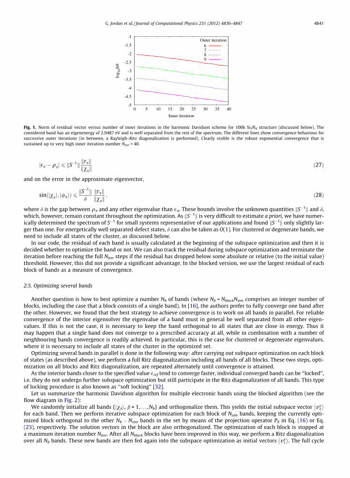
Fig. 1. Norm of residual vector versus number of inner iterations in the harmonic Davidson scheme for 100k Si3N4 structure (discussed below). Theconsidered band has an eigenenergy of 2.9487 eV and is well separated from the rest of the spectrum. The different lines show convergence behaviour forsuccessive outer iterations (in between, a Rayleigh–Ritz diagonalization is performed). Clearly visible is the robust exponential convergence that issustained up to very high inner iteration number Niter = 40.

G. Jordan et al. / Journal of Computational Physics 231 (2012) 4836–4847 4841

j�a � qaj 6 kS�1k krakkvak

ð27Þ

and on the error in the approximate eigenvector,

sinðjvai; j/aiÞ 6kS�1k

dkrakkvak

; ð28Þ

where d is the gap between qa and any other eigenvalue than �a. These bounds involve the unknown quantities kS�1k and d,which, however, remain constant throughout the optimization. As kS�1k is very difficult to estimate a priori, we have numer-ically determined the spectrum of S�1 for small systems representative of our applications and found kS�1k only slightly lar-ger than one. For energetically well separated defect states, d can also be taken as O(1). For clustered or degenerate bands, weneed to include all states of the cluster, as discussed below.

In our code, the residual of each band is usually calculated at the beginning of the subspace optimization and then it isdecided whether to optimize the band or not. We can also track the residual during subspace optimization and terminate theiteration before reaching the full Niter steps if the residual has dropped below some absolute or relative (to the initial value)threshold. However, this did not provide a significant advantage. In the blocked version, we use the largest residual of eachblock of bands as a measure of convergence.

2.5. Optimizing several bands

Another question is how to best optimize a number Nb of bands (where Nb = NblockNsim comprises an integer number ofblocks, including the case that a block consists of a single band). In [16], the authors prefer to fully converge one band afterthe other. However, we found that the best strategy to achieve convergence is to work on all bands in parallel. For reliableconvergence of the interior eigensolver the eigenvalue of a band must in general be well separated from all other eigen-values. If this is not the case, it is necessary to keep the band orthogonal to all states that are close in energy. Thus itmay happen that a single band does not converge to a prescribed accuracy at all, while in combination with a number ofneighbouring bands convergence is readily achieved. In particular, this is the case for clustered or degenerate eigenvalues,where it is necessary to include all states of the cluster in the optimized set.

Optimizing several bands in parallel is done in the following way: after carrying out subspace optimization on each blockof states (as described above), we perform a full Ritz diagonalization including all bands of all blocks. These two steps, opti-mization on all blocks and Ritz diagonalization, are repeated alternately until convergence is attained.

As the interior bands closer to the specified value �ref tend to converge faster, individual converged bands can be ‘‘locked’’,i.e. they do not undergo further subspace optimization but still participate in the Ritz diagonalization of all bands. This typeof locking procedure is also known as ‘‘soft locking’’ [32].

Let us summarize the harmonic Davidson algorithm for multiple electronic bands using the blocked algorithm (see theflow diagram in Fig. 2):

We randomly initialize all bands {jvbi, b = 1, . . . ,Nb} and orthogonalize them. This yields the initial subspace vector va1

�� �for each band. Then we perform iterative subspace optimization for each block of Nsim bands, keeping the currently opti-mized block orthogonal to the other Nb � Nsim bands in the set by means of the projection operator PX in Eq. (16) or Eq.(23), respectively. The solution vectors in the block are also orthogonalized. The optimization of each block is stopped ata maximum iteration number Niter. After all Nblock blocks have been improved in this way, we perform a Ritz diagonalizationover all Nb bands. These new bands are then fed again into the subspace optimization as initial vectors va

1

�� �. The full cycle

Fig. 2. Flow diagram of our implementation of the harmonic Davidson algorithm.

4842 G. Jordan et al. / Journal of Computational Physics 231 (2012) 4836–4847

subspace optimization/Ritz diagonalization is continued until a specified threshold for the residual has been reached (or upto a given maximum number of Nelm repetitions).

3. Examples

As the benchmark in accuracy and speed of the newly implemented harmonic Davidson algorithm we choose the conven-tional Davidson method, which is the default algorithm used in VASP. The main difference to the harmonic version is that con-ventional Davidson uses the standard orthogonal projection method Eq. (8). For a detailed explanation we refer to [23]. Thus,for the reasons explained in the introduction, the conventional Davidson approach is in general not suited for interior eigen-problems. To compute selected bands around some energy �ref, one needs to include all bands below �ref and a considerablenumber of excess bands above this energy in the calculation. But the Rayleigh–Ritz diagonalization over all bands, which isrequired after subspace optimization of each individual band both in harmonic and conventional Davidson, scales like N3

b . As aconsequence, for small systems and small Nb, conventional Davidson still outperforms the harmonic one because inclusion ofall bands improves the conditioning of the eigenproblem. However, for large system sizes, the cubic scaling of Rayleigh–Ritzdiagonalization dominates compute time and hence conventional Davidson calculations are practically unfeasible beyond a

G. Jordan et al. / Journal of Computational Physics 231 (2012) 4836–4847 4843

few thousand atoms. The reduction of Nb that the harmonic Davidson makes possible is crucial in this case. A second impor-tant issue is the huge memory size that would be required to store all bands.

VASP is written in FORTRAN, and uses BLAS/LAPACK for linear algebra operations, FFTW for fast Fourier transforms andMPI for parallelization. In parallel execution, we switch between distribution of electron bands and distribution of planewave coefficients depending on which is more efficient. Computations were run on a local cluster equipped with 4 nodesof 8 Intel Xeon CPUs with 2.67 GHz and 4 GB RAM per CPU.

3.1. Si3N4 with vacancies – isolated eigenvalues

For our first test system we chose a randomized Si3N4 sample with two geometric defects. It was produced by randomlyshifting atomic positions of an a-Si3N4 supercell, with a maximum displacement of 0.05 Å, and creating one Si and one Nvacancy.

The electronic structure is determined non-selfconsistently. The fixed, non-selfconsistent charge density is obtained byfitting atom centered densities to the charge density of a self-consistent reference calculation for amorphous Si3N4. Our fit-ting functions are two Gaussians for each atomic species, Si and N. Details of this procedure will be described in a separatepublication [33]. In general, the procedure yields band structures within a few percent of full self-consistent DFT calculationsfor all polymorphs of bulk Si3N4, and even the densities of states of amorphous model structures are well reproduced. For thepurpose of this test, the defect structures were not relaxed, and spin polarization was not taken into account, since our focalpoint here is whether the iterative matrix diagonalization works reliably for states close to the valence band maximum(VBM) and conduction band minimum (CBM).

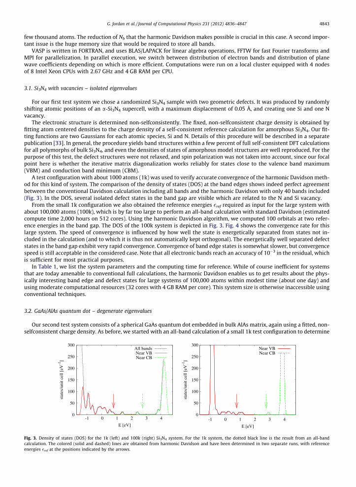
A test configuration with about 1000 atoms (1k) was used to verify accurate convergence of the harmonic Davidson meth-od for this kind of system. The comparison of the density of states (DOS) at the band edges shows indeed perfect agreementbetween the conventional Davidson calculation including all bands and the harmonic Davidson with only 40 bands included(Fig. 3). In the DOS, several isolated defect states in the band gap are visible which are related to the N and Si vacancy.

From the small 1k configuration we also obtained the reference energies �ref required as input for the large system withabout 100,000 atoms (100k), which is by far too large to perform an all-band calculation with standard Davidson (estimatedcompute time 2,000 hours on 512 cores). Using the harmonic Davidson algorithm, we computed 100 orbitals at two refer-ence energies in the band gap. The DOS of the 100k system is depicted in Fig. 3. Fig. 4 shows the convergence rate for thislarge system. The speed of convergence is influenced by how well the state is energetically separated from states not in-cluded in the calculation (and to which it is thus not automatically kept orthogonal). The energetically well separated defectstates in the band gap exhibit very rapid convergence. Convergence of band edge states is somewhat slower, but convergencespeed is still acceptable in the considered case. Note that all electronic bands reach an accuracy of 10�3 in the residual, whichis sufficient for most practical purposes.

In Table 1, we list the system parameters and the computing time for reference. While of course inefficient for systemsthat are today amenable to conventional full calculations, the harmonic Davidson enables us to get results about the phys-ically interesting band edge and defect states for large systems of 100,000 atoms within modest time (about one day) andusing moderate computational resources (32 cores with 4 GB RAM per core). This system size is otherwise inaccessible usingconventional techniques.

3.2. GaAs/AlAs quantum dot – degenerate eigenvalues

Our second test system consists of a spherical GaAs quantum dot embedded in bulk AlAs matrix, again using a fitted, non-selfconsistent charge density. As before, we started with an all-band calculation of a small 1k test configuration to determine

0

50

100

150

200

250

300

-1 0 1 2 3 4

stat

es/u

nit c

ell [

eV-1

]

E [eV]

All bandsNear VBNear CB

0

50

100

150

200

250

300

-1 0 1 2 3 4

stat

es/u

nit c

ell [

eV-1

]

E [eV]

Near VBNear CB

Fig. 3. Density of states (DOS) for the 1k (left) and 100k (right) Si3N4 system. For the 1k system, the dotted black line is the result from an all-bandcalculation. The colored (solid and dashed) lines are obtained from harmonic Davidson and have been determined in two separate runs, with referenceenergies �ref at the positions indicated by the arrows.

-4

-2

0

2

4

6

0 5 10 15 20

log 1

0||r|

|

log 1

0||r|

|

Iteration

2.9487 eV3.8384 eV3.8388 eV3.8549 eV3.8553 eV3.8555 eV3.8561 eV3.8564 eV3.8571 eV3.8579 eV

-4

-2

0

2

4

6

0 5 10 15 20Iteration

-0.8347 eV-0.6049 eV-0.5691 eV-0.2131 eV-0.0425 eV 0.1728 eV 0.3032 eV 0.5565 eV 0.9612 eV 1.1527 eV

Fig. 4. Convergence of the norm of the residual vector versus the number of outer iterations for the 100k Si3N4 system. Left: VBM (�ref = 0.78). Right: CBM(�ref = 2.78). In each outer iteration, each vector in the set is optimized 40 times. The calculations included 100 bands for each reference energy, and weshow the residual only for the ten highest (VBM) and lowest (CBM) bands, respectively. Robust convergence is achieved for these bands. A residual of 10�3 isufficient for most practical purposes.

Table 1System parameters (number of atoms) for the small (1k) and large (100k) Si3N4 configurations. The atompositions have been slightly randomized and one Si and one N atom have been replaced by vacancies.

System (Si3N4) units Total atoms Electrons

1k 144 1006 4599100k 14,112 98,782 451,575

Table 2Computation times for the Si3N4 system for the conventional Davidson and the harmonic Davidson algorithm. The number of plane waves is equal to tdimension of the Hamiltonian matrix H, although this matrix is never formed explicitly in the code. The number of inner iterations corresponds to the numbof matrix–vector products Hjvi. For the harmonic Davidson algorithm, the number of inner iterations is Niter = 40 per band, and after 20 outer iterationsbands are well converged.

System Algorithm Plane waves No. of bands Cores Cpu time (excl. setup) Total no. of inner iterations

1k Davidson 22,000 2804 24 4 min 52,0001k Harmonic Davidson 22,000 40 16 7 min 32,000100k Harmonic Davidson 2.1 mio. 100 32 30 h 80,000

Table 3System parameters (number of atoms) for the spherical GaAs quantum dot embedded in a cubic AlAs supercell.

System Ga Al As Total atoms Electrons

1k 135 365 500 1000 4000100k 13,811 41,485 55,296 110,592 442,368

4844 G. Jordan et al. / Journal of Computational Physics 231 (2012) 4836–4847

s

heerall

the approximate position of the valence and conduction band edge, and use this in the harmonic Davidson calculation of a100k system. System parameters are given in Table 3. The larger GaAs nanodot has a radius of about 53 Å.

For the 1k system, we find the valence band maximum (VBM) at �0.47 eV, and the conduction band minimum (CBM) at1.04 eV. Since GaAs has a smaller band gap than AlAs, the GaAs quantum dot creates many states that are spatially localizedon the GaAs quantum dot. Our goal is the calculation of these states, which behave essentially like electronic states in aspherical confinement potential. In this case the main problem is that these confined impurity states form a fairly densespectrum. Because of the high symmetry of the problem many states belong to degenerate doublets or triplets, and evensix times degenerate states are observed. Such degeneracies are expected to pose increased difficulties to an inner eigen-problem solver.

In Fig. 5 we show the convergence for the 1k system for the ten states closest to VBM and CBM, both with respect to theenergy and the norm of the residual krk, confirming reliable convergence to the correct result for all bands. This example alsoclearly demonstrates that energy convergence is usually faster than convergence of the residual. For comparison, we deter-mined one valence band and conduction band edge state using a single band calculation and �ref = 0.02 and �ref = 0.52, respec-tively, (marked by ‘‘1 band’’ in the legend). In this case, convergence speed is considerably reduced.

Convergence rates for the large 100k system are shown in Fig. 6. Since there is a high density of states at the valence bandedge, we have included more bands (200 instead of 100) to accelerate convergence. System parameters and the computingtimes for the GaAs/AlAs quantum dot are listed in Table 4.

-4

-3

-2

-1

0

1

2

0 5 10 15 20

log 1

0|ε

- ε t

rue|

Iteration

1 band: -0.4741 eV40 bands: -0.4741 eV

-0.4741 eV-0.4741 eV-0.5801 eV-0.5801 eV-0.5802 eV-0.6175 eV-0.6175 eV-0.6802 eV-0.6802 eV

-4

-3

-2

-1

0

1

2

0 5 10 15 20

log 1

0|ε

- ε t

rue|

Iteration

1 band: 1.0467 eV40 bands: 1.0467 eV

1.1987 eV1.1987 eV1.1987 eV1.4048 eV1.4049 eV1.4049 eV1.4049 eV1.4049 eV1.4137 eV

-4

-2

0

2

4

6

0 5 10 15 20

log 1

0||r|

|

Iteration

1 band: -0.4741 eV40 bands: -0.4741 eV

-0.4741 eV-0.4741 eV-0.5801 eV-0.5801 eV-0.5802 eV-0.6175 eV-0.6175 eV-0.6802 eV-0.6802 eV

-5

-4

-3

-2

-1

0

1

2

0 5 10 15 20

log 1

0||r|

|

Iteration

1 band: 1.0467 eV40 bands: 1.0467 eV

1.1987 eV1.1987 eV1.1987 eV1.4048 eV1.4049 eV1.4049 eV1.4049 eV1.4049 eV1.4137 eV

Fig. 5. Convergence of the eigenenergy (top row) and norm of the residual vector (bottom row) versus the number of outer iterations for a small 1k GaAs/AlAs quantum dot using harmonic Davidson algorithm. Left column: VB maximum, Right column: CB minimum. In each outer iteration, each vector in theset consisting of 40 vectors is optimized 40 times. For the 1 band calculations, a single band was calculated with �ref = 0.02 (VBM) or �ref = 0.52 (CBM). Forthe 40 band calculation, a single reference energy �ref = 0.52 was used.

-4

-2

0

2

4

6

0 5 10 15 20

log 10

||r||

Iteration

0.7205 eV0.8561 eV0.8561 eV0.8561 eV0.9875 eV0.9875 eV0.9875 eV0.9958 eV0.9958 eV1.0519 eV

-4

-2

0

2

4

6

0 5 10 15 20

log 10

||r||

Iteration

-0.1346 eV -0.1320 eV -0.1320 eV -0.1319 eV -0.1266 eV -0.1266 eV -0.1266 eV -0.1180 eV -0.1180 eV -0.1180 eV

Fig. 6. Convergence of the norm of the residual vector versus the number of outer iterations for the large 100k GaAs/AlAs quantum dot. Left: VB maximum(�ref = �0.08), Right: CB minimum (�ref = 0.72).

Table 4Computation times for the GaAs/AlAs quantum dot. Parameters as in Table 2. Comparison with Table 2 shows that the harmonic Davidson algorithm scalesroughly linearly both with the number of plane waves and the number of bands. The calculation for the 100k quantum dot was repeated with 200 bands toimprove convergence of the dense states at the VBM.

System Algorithm Plane waves No. of bands Cores Cpu time (excl. setup) Total no. of inner iterations

1k Davidson 42,000 2504 16 26 min 65,0001k Harmonic Davidson 42,000 40 16 20 min 32,000100k Harmonic Davidson 4.7 mio. 200/100 32 122/55 h 160,000/80,000

G. Jordan et al. / Journal of Computational Physics 231 (2012) 4836–4847 4845

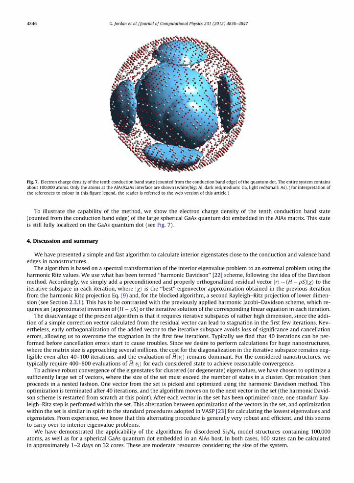
Fig. 7. Electron charge density of the tenth conduction band state (counted from the conduction band edge) of the quantum dot. The entire system containsabout 100,000 atoms. Only the atoms at the AlAs/GaAs interface are shown (white/big: Al, dark red/medium: Ga, light red/small: As). (For interpretation ofthe references to colour in this figure legend, the reader is referred to the web version of this article.)

4846 G. Jordan et al. / Journal of Computational Physics 231 (2012) 4836–4847

To illustrate the capability of the method, we show the electron charge density of the tenth conduction band state(counted from the conduction band edge) of the large spherical GaAs quantum dot embedded in the AlAs matrix. This stateis still fully localized on the GaAs quantum dot (see Fig. 7).

4. Discussion and summary

We have presented a simple and fast algorithm to calculate interior eigenstates close to the conduction and valence bandedges in nanostructures.

The algorithm is based on a spectral transformation of the interior eigenvalue problem to an extremal problem using theharmonic Ritz values. We use what has been termed ‘‘harmonic Davidson’’ [22] scheme, following the idea of the Davidsonmethod. Accordingly, we simply add a preconditioned and properly orthogonalized residual vector jri � (H � qS)jvi to theiterative subspace in each iteration, where jvi is the ‘‘best’’ eigenvector approximation obtained in the previous iterationfrom the harmonic Ritz projection Eq. (9) and, for the blocked algorithm, a second Rayleigh–Ritz projection of lower dimen-sion (see Section 2.3.1). This has to be contrasted with the previously applied harmonic Jacobi–Davidson scheme, which re-quires an (approximate) inversion of (H � qS) or the iterative solution of the corresponding linear equation in each iteration.

The disadvantage of the present algorithm is that it requires iterative subspaces of rather high dimension, since the addi-tion of a simple correction vector calculated from the residual vector can lead to stagnation in the first few iterations. Nev-ertheless, early orthogonalization of the added vector to the iterative subspace avoids loss of significance and cancellationerrors, allowing us to overcome the stagnation in the first few iterations. Typically we find that 40 iterations can be per-formed before cancellation errors start to cause troubles. Since we desire to perform calculations for huge nanostructures,where the matrix size is approaching several millions, the cost for the diagonalization in the iterative subspace remains neg-ligible even after 40–100 iterations, and the evaluation of eHjv ji remains dominant. For the considered nanostructures, wetypically require 400–800 evaluations of eHjv ji for each considered state to achieve reasonable convergence.

To achieve robust convergence of the eigenstates for clustered (or degenerate) eigenvalues, we have chosen to optimize asufficiently large set of vectors, where the size of the set must exceed the number of states in a cluster. Optimization thenproceeds in a nested fashion. One vector from the set is picked and optimized using the harmonic Davidson method. Thisoptimization is terminated after 40 iterations, and the algorithm moves on to the next vector in the set (the harmonic David-son scheme is restarted from scratch at this point). After each vector in the set has been optimized once, one standard Ray-leigh–Ritz step is performed within the set. This alternation between optimization of the vectors in the set, and optimizationwithin the set is similar in spirit to the standard procedures adopted in VASP [23] for calculating the lowest eigenvalues andeigenstates. From experience, we know that this alternating procedure is generally very robust and efficient, and this seemsto carry over to interior eigenvalue problems.

We have demonstrated the applicability of the algorithms for disordered Si3N4 model structures containing 100,000atoms, as well as for a spherical GaAs quantum dot embedded in an AlAs host. In both cases, 100 states can be calculatedin approximately 1–2 days on 32 cores. These are moderate resources considering the size of the system.

G. Jordan et al. / Journal of Computational Physics 231 (2012) 4836–4847 4847

The design of an efficient matrix diagonalization scheme for interior eigenvalue problems is only one issue that needs tobe addressed in order to calculate the electronic properties of large nanostructures. Because the present scheme can onlycalculate few selected states close the conduction and valence band edges, the standard selfconsistent density functionaltheory procedure cannot be applied. This procedure requires the calculation of all occupied states, a task not routinely pos-sible for systems containing more than 10,000 atoms. To circumvent this problem, we have constructed effective screenedpotentials that allow to calculate the band structure of Si3N4, GaAs and AlAs with few percent accuracy without the need forselfconsistency. The construction of the screened potentials proceeds via fitting Gaussian atom centered charge densities tothe selfconsistent charge density of amorphous model structures [33]. Open issues concern local relaxations and stress andstrain effects, which will be addressed in later work.

Acknowledgements

The research leading to these results has received funding from the European Community’s 7th Framework Programmeunder grant agreement no. 228513 (HiperSol) and from the Austrian Science Fund (FWF) within the SFB IRON.

References

[1] Stefan Goedecker, Linear scaling electronic structure methods, Reviews of Modern Physics 71 (4) (1999) 1085.[2] E. Hernández, M.J. Gillan, C.M. Goringe, Linear-scaling density-functional-theory technique: the density-matrix approach, Physical Review B 53 (11)

(1996) 7147.[3] M.J. Gillan, D.R. Bowler, A.S. Torralba, T. Miyazaki, Order-N first-principles calculations with the conquest code, Computer Physics Communications 177

(1–2) (2007) 14–18.[4] José M. Soler, Emilio Artacho, Julian D. Gale, Alberto García, Javier Junquera, Pablo Ordejón, Daniel Sánchez-Portal, The SIESTA method for ab initio

order-n materials simulation, Journal of Physics: Condensed Matter 14 (11) (2002) 2745–2779.[5] Chris-Kriton Skylaris, Peter D. Haynes, Arash A. Mostofi, Mike C. Payne, Introducing ONETEP: linear-scaling density functional simulations on parallel

computers, The Journal of Chemical Physics 122 (8) (2005) 084119.[6] D.R. Bowler, T. Miyazaki, Calculations for millions of atoms with density functional theory: linear scaling shows its potential, Journal of Physics:

Condensed Matter 22 (7) (2010) 074207.[7] Lin-Wang Wang, Alex Zunger, Electronic structure pseudopotential calculations of large (apprx. 1000 atoms) Si quantum dots, The Journal of Physical

Chemistry 98 (8) (1994) 2158–2165.[8] Lin-Wang Wang, Alex Zunger, Local-density-derived semiempirical pseudopotentials, Physical Review B 51 (24) (1995) 17398.[9] Lin-Wang Wang, Alex Zunger, Linear combination of bulk bands method for large-scale electronic structure calculations on strained nanostructures,

Physical Review B 59 (24) (1999) 15806.[10] David Vanderbilt, Soft self-consistent pseudopotentials in a generalized eigenvalue formalism, Physical Review B 41 (11) (1990) 7892.[11] P.E. Blöchl, Projector augmented-wave method, Physical Review B 50 (24) (1994) 17953.[12] G. Kresse, D. Joubert, From ultrasoft pseudopotentials to the projector augmented-wave method, Physical Review B 59 (3) (1999) 1758.[13] Y. Saad, Basic ideas, in: Z. Bai, J. Demmel, J. Dongarra, A. Ruhe, H. van der Vorst (Eds.), Templates for the Solution of Algebraic Eigenvalue Problems: A

Practical Guide, SIAM, Philadelphia, 2000.[14] Ronald B. Morgan, Min Zeng, Harmonic projection methods for large non-symmetric eigenvalue problems, Numerical Linear Algebra with Applications

5 (1) (1998) 33–55.[15] Lin-Wang Wang, Alex Zunger, Solving Schrödinger’s equation around a desired energy: application to silicon quantum dots, The Journal of Chemical

Physics 100 (3) (1994) 2394.[16] Alan R. Tackett, Massimiliano Di Ventra, Targeting specific eigenvectors and eigenvalues of a given Hamiltonian using arbitrary selection criteria,

Physical Review B 66 (24) (2002) 245104.[17] R. Lehoucq, D. Sorensen, Spectral transformations, in: Z. Bai, J. Demmel, J. Dongarra, A. Ruhe, H. van der Vorst (Eds.), Templates for the Solution of

Algebraic Eigenvalue Problems: A Practical Guide, SIAM, Philadelphia, 2000.[18] Ronald B. Morgan, Computing interior eigenvalues of large matrices, Linear Algebra and its Applications 154-156 (1991) 289–309.[19] Chris C. Paige, Beresford N. Parlett, Henk A. van der Vorst, Approximate solutions and eigenvalue bounds from Krylov subspaces, Numerical Linear

Algebra with Applications 2 (2) (1995) 115–133.[20] Gerard L.G. Sleijpen, Henk A. van der Vorst, A Jacobi–Davidson iteration method for linear eigenvalue problems, SIAM Journal on Matrix Analysis and

Applications 17 (2) (1996) 401.[21] Diederik R. Fokkema, Gerard L.G. Sleijpen, Henk A. van der Vorst, Jacobi–Davidson style QR and QZ algorithms for the reduction of matrix pencils, SIAM

Journal on Scientific Computing 20 (1) (1998) 94.[22] Jonathan J. Dorando, Johannes Hachmann, Garnet Kin-Lic Chan, Targeted excited state algorithms, The Journal of Chemical Physics 127 (8) (2007)

084109.[23] G. Kresse, J. Furthmüller, Efficiency of ab-initio total energy calculations for metals and semiconductors using a plane-wave basis set, Computational

Materials Science 6 (1) (1996) 15–50.[24] D.M. Wood, A. Zunger, A new method for diagonalising large matrices, Journal of Physics A Mathematical General 18 (1985) 1343–1359.[25] Péter Pulay, Convergence acceleration of iterative sequences: the case of SCF iteration, Chemical Physics Letters 73 (2) (1980) 393–398.[26] Y. Saad, Numerical Methods for Large Eigenvalue Problems, Manchester University Press, 1991.[27] Michael P. Teter, Michael C. Payne, Douglas C. Allan, Solution of Schrödinger’s equation for large systems, Physical Review B 40 (18) (1989) 12255.[28] Andreas Stathopoulos, Yousef Saad, Kesheng Wu, Dynamic thick restarting of the Davidson and the implicitly restarted Arnoldi methods, SIAM Journal

on Scientific Computing 19 (1996) 227–245.[29] Christopher W. Murray, Stephen C. Racine, Ernest R. Davidson, Improved algorithms for the lowest few eigenvalues and associated eigenvectors of

large matrices, Journal of Computational Physics 103 (2) (1992) 382–389.[30] Andreas Stathopoulos, Yousef Saad, Restarting techniques for the (Jacobi–)Davidson symmetric eigenvalue methods, Electronic Transactions on

Numerical Analysis 7 (1998) 163–181.[31] Z. Bai, R. Li, Stability and accuracy assessments, in: Z. Bai, J. Demmel, J. Dongarra, A. Ruhe, H. van der Vorst (Eds.), Templates for the Solution of

Algebraic Eigenvalue Problems: A Practical Guide, S IAM, Philadelphia, 2000.[32] A.V. Knyazev, M.E. Argentati, I. Lashuk, E.E. Ovtchinnikov, Block locally optimal preconditioned eigenvalue xolvers (BLOPEX) in hypre and PETSc, SIAM

Journal on Scientific Computing 29 (5) (2007) 2224.[33] M. Marsman, G. Jordan, L.-E. Hintzsche, Y.-S. Kim, G. Kresse, Gaussian charge-transfer charge distributions for non-self-consistent electronic structure

calculations, Physical Review B 85 (11) (2012) 115122.