WHEN WORK MOVES:

JOB SUBURBANIZATION AND BLACK EMPLOYMENT

Conrad Miller∗

This Version: May 2021

Abstract

This paper examines whether job suburbanization caused declines in black employment

rates from 1970 to 2000. I find that black workers are less likely than white workers to work

in observably similar jobs that are located further from the central city. Using evidence from

establishment relocations, I find that this relationship at least in part reflects the causal effect of

job location. At the local labor market level, I find that job suburbanization is associated with

substantial declines in black employment rates relative to white employment rates. Evidence

from nationally planned highway infrastructure corroborates a causal interpretation.

∗Haas School of Business and Department of Economics, University of California, Berkeley (email:ccmiller@berkeley.edu). I thank David Autor, Will Dobbie, Ben Feigenberg, Amy Finkelstein, Heidi Williams, SethZimmerman, and seminar participants at Princeton, Chicago Harris, Ohio State, Upjohn Institute, the 2015 EALE-SOLE conference, the 2012 AEA Summer Pipeline Conference, and MIT labor lunch for comments. I thank NathanielBaum-Snow for providing access to highway data compiled for Baum-Snow (2007). I also thank Ron Edwards, BlissCartwright, and Georgianna Hawkins of the Equal Employment Opportunity Commission for facilitating access to theEEO-1 form data and providing helpful feedback.

1

1 Introduction

Over the last 60 years in the United States, the unemployment rate among black working-age adults

has roughly doubled the national unemployment rate (Fairlie and Sundstrom, 1999).1 The spatial

mismatch hypothesis, introduced by Kain (1968) and further popularized by Wilson (1987) and

Wilson (1996), attributes racial disparities in employment rates in part to spatial frictions in the

labor and housing markets. Under this theory, black households tend to live relatively far from

work opportunities, reducing their access to gainful employment. This distance increased after

World War II, as firms and white households began relocating from central cities to suburban rings

at an accelerated pace.2 Black households, who faced discrimination in housing and mortgage

markets (Yinger, 1995; Rothstein, 2017), remained concentrated in central cities.3 As a result,

black households tend to live further away from the portions of metropolitan areas experiencing

substantial job growth, depressing their labor market outcomes. For example, between 1970 and

2000 in the sample of metropolitan areas studied here, the employment rate for black men declined

by about 10% more than the employment rate for white men.4

It remains unclear whether job suburbanization and the decline of black employment over this

period are causally linked, however. Though researchers have posited several explanations for why

work has decentralized, including improvements in transportation technology and infrastructure,

land costs, and worker suburbanization (Glaeser and Kahn, 2001), the process of job suburbaniza-

tion is not well understood. Job suburbanization may be associated with changes in labor demand

and supply that would generate changes in the racial composition of the workforce even in the ab-

sence of suburbanization. Moreover, even if firms began to locate in the suburbs due to exogenous

1Large disparities remain conditional on education and Armed Forces Qualification Test (AFQT) scores, a commonproxy for labor market skills (Ritter and Taylor, 2011).

2In 1960, 61% of metropolitan area jobs were in the central city; by 2000, the central city share declined to 34%(Baum-Snow, forthcoming).

3In 1940, in 14 of the largest metropolitan areas, 78.5% and 61.9% of black and white residents lived in thecentral city. By 2000, these shares declined to 66.5% and 26.6%. The 14 metropolitan areas are the following:Baltimore, Boston, Buffalo-Niagara Falls, Chicago, Detroit, Houston, Los Angeles-Long Beach, Minneapolis-St.Paul, New York, Philadelphia, Pittsburgh, St. Louis, San Francisco-Oakland, and Washington, DC. I limit to these 14metropolitan areas because they are consistently identified in census and Current Population Survey microdata.

4Among women, the employment rate for white women increased by about 34% more than the employment ratefor black women.

2

factors, it is not clear what implications this would have for the racial composition of the work-

force. While the segregation of black households in the central city has been a persistent feature

of U.S. metropolitan areas (Cutler et al., 1999), workers may respond to the changing geography

of work by changing jobs, altering their commute, or moving to a different neighborhood. These

response margins may be sufficient for job suburbanization to have little effect on labor market

outcomes by race.

In this paper I examine whether job suburbanization caused significant declines in black em-

ployment from 1970 to 2000. I provide both job-level and local labor market-level evidence. At

the job level, I find that black workers are less likely than white workers to work in observably

similar jobs located further from the central city. Using evidence from establishment relocations,

I find that this relationship at least in part reflects the causal effect of job location. At the local

labor market level, I find that job suburbanization is associated with substantial declines in black

employment rates relative to white employment rates. Evidence from nationally planned highway

infrastructure corroborates a causal interpretation. My findings imply that job suburbanization can

explain the majority of the relative decline in black men’s employment over this period.

After I introduce the data and how I measure job suburbanization (Section 2), the analysis is

divided into two sections. In the job-level analysis (Section 3), I use establishment-level adminis-

trative data from the Equal Employment Opportunity Commission to show that black workers are

substantially less likely than white workers to work in jobs located further from the central city. In

particular, conditional on job characteristics, the black share of employees in metropolitan area es-

tablishments is decreasing in an establishment’s distance from the central business district (CBD).

Remarkably, this spatial segregation is stable over time despite widespread movement of popula-

tion and jobs to the suburbs. I also provide additional evidence that this spatial segregation reflects

at least in part the causal effect of job location on racial composition. I show that the relationship

between job location and racial composition holds within firms that operate multiple establish-

ments within a metropolitan area. I also find that establishments that relocate from the central city

to the suburbs experience sharp coincident declines in the black share of their employees despite

3

no significant changes in their occupational composition.

This persistent spatial segregation suggests job suburbanization may have reduced black em-

ployment rates. Effect size estimates from establishment relocations suggest that job suburbaniza-

tion decreased the black share of the workforce by 2.3% each decade. However, suburbanization

may be offset in the aggregate by worker re-sorting across workplaces. This motivates the second

portion of the analysis (Section 4), which examines the relationship between job suburbanization

and black employment across local labor markets.

Using census data and a synthetic panel, differences-in-differences research design, I find that

job suburbanization is associated with substantial declines in black employment rates relative to

white employment rates. For every 10% decline in the fraction of metropolitan statistical area

(MSA) jobs located in the central city over this period, black relative employment rates declined

by 1.6% to 2.3%, while white employment rates increased by a (statistically insignificant) 0.3%

to 0.4%. This relationship holds within observable skill groups, and estimates are similar for men

and women. Relative earnings declined by 1.2% to 2.3%, though these estimates are less stable

across specifications.

To address the potential endogeneity of job suburbanization—in particular, changes in the spa-

tial distribution of work driven by unobserved labor supply shocks that are unevenly distributed

across black and white working-age adults—I instrument for job suburbanization using variation

in nationally planned interstate highway construction across MSAs as identified in Baum-Snow

(2007). These highways were planned in the 1940s and 1950s and were primarily designed to

link faraway places rather than to facilitate local commuting or economic development. Hence,

their assignment across MSAs should be exogenous to residual labor supply shocks from 1970 to

2000. While highways have a variety of effects on the labor market that may potentially violate

the exclusion restriction, I argue that they are unrelated to labor demand and supply shocks that

would disproportionately affect black workers, the most concerning omitted variables. In particu-

lar, suburbanization induced by highway construction is not related to changes in local industry or

occupation mix that would portend changes in black relative employment rates.

4

Consistent with Baum-Snow (forthcoming), I find that each highway ray emanating from the

central city leads to a 7%–10% decline in the fraction of MSA jobs located in the central city

from 1970 to 2000. In turn, interstate highways caused declines in black relative employment

rates, with highway-based instrumental variable (IV) estimates for the relationship between job

suburbanization and black employment rates that are comparable to the ordinary least squares

(OLS) estimates. I conclude that job suburbanization was an important determinant of black-white

labor market inequality from 1970 to 2000. The estimates imply that job suburbanization can

explain over half of the relative decline in black men’s employment rates and 15%–20% of the

increase in white women’s employment rates relative to black women’s over this period.

While this paper provides novel evidence on spatial segregation in the labor market and the

causal effect of workplace location on the racial composition of employees, it is largely silent

on why space matters. I discuss potential mechanisms in Section 5. Black adults may be less

likely to work in the suburbs due to commuting costs, job search costs, or employer preferences.

A key implication of this paper is that the relationship between job suburbanization and black

employment is not driven by changes in firm demand for worker skills. Interestingly, the labor

market is substantially less spatially segregated than the housing market, so commuting flows do

offset residential segregation to some degree. However, while black households are residentially

less concentrated in central city neighborhoods then they were in 1970, this movement has not

been sufficient to noticeably alter the spatial segregation of the labor market.

This paper contributes to an extensive literature testing the spatial mismatch hypothesis. Prior

work typically relates labor market outcomes to measures of job accessibility in a cross-section

(see Ihlanfeldt and Sjoquist, 1998 for a review of the older literature).5 Most recent work in this

literature finds some support for spatial mismatch, though there has been considerable debate about

its empirical importance (Ellwood, 1986). The results tend to be sensitive to how job accessibility

5Three exceptions are Mouw (2000), Weinberg et al. (2004), and Stoll (2006). Mouw (2000) estimates the rela-tionship between changes in job density and neighborhood-level employment rates in Chicago and Detroit from 1980to 1990. Weinberg et al. (2004) exploit individual moves across neighborhoods using the 1979 National LongitudinalSurvey of Youth. Both papers find evidence of spatial mismatch. Stoll (2006) relates changes in job sprawl to changesin spatial mismatch between where black households reside and employers are located across MSAs from 1990 to2000 and finds no detectable relationship.

5

is measured (Raphael, 1998).6 More importantly, results from this literature are made difficult to

interpret by the endogeneity of household and firm location. Residents who are less productive

may sort into neighborhoods farther from work opportunities, where rents are typically lower.7

Similarly, firms may choose to locate in neighborhoods with residents who are more productive.

In this paper, I take a more “reduced-form” approach—rather than attempt to estimate the effects

of work proximity per se, I estimate the effects of job suburbanization at the local labor market

level.8

This paper also contributes to a smaller literature that studies how a work establishment’s lo-

cation influences the racial composition of its employees. This research has found that location

appears to be an important determinant of employee composition. However, prior work has been

limited to relatively small samples—cross-sectional studies of a few thousand firms in a handful of

metropolitan areas (Holzer and Ihlanfeldt, 1996) or case studies of individual plant relocations (Zax

and Kain, 1996; Fernandez, 2008). By contrast, the administrative data used here cover hundreds

of thousands of establishments for several decades, including thousands of relocation episodes.

2 Data and Measurement

In this paper I use three data sources: establishment-level data from EEO-1 forms, individual-level

and city-level census data, and MSA-level data on the interstate highway system from Baum-Snow

(2007). In this section I describe each data source and introduce my MSA-level measure of job

suburbanization.6For example, previous researchers have used the local job density, local job growth, and the average commuting

times of local workers as measures of job accessibility. Hellerstein et al. (2008) argue that accessibility measuresshould be race specific; for example, the density of jobs into which black workers are hired is a more relevant acces-sibility metric for black jobseekers than job density per se.

7Alternatively, if spatial frictions are relevant, residents who find it difficult to obtain work may sort into neighbor-hoods with higher employment density.

8Andersson et al. (2018) is an important and recent contribution to this literature. The authors use matchedemployer-employee data to study the relationship between job accessibility and jobless duration among workers dis-placed in mass layoffs. They find that, among similar job searchers, search duration is decreasing in job accessibility.However, Andersson et al. do not study how job accessibility contributes to racial differences in labor market out-comes or the effects of job suburbanization more generally. I view the approaches of Andersson et al. (2018) and thecurrent paper as complimentary.

6

2.1 EEO-1 Form Data

For the job-level analysis, I use a unique set of establishment-level panel data. These data, known

as EEO-1 form data, are collected by the U.S. Equal Employment Opportunity Commission (EEOC)

and cover the years 1971–2000. As part of the Civil Rights Act of 1964, firms meeting certain size

requirements are required to complete EEO-1 forms annually and submit them to the EEOC. Firms

are required to report their overall racial, ethnic, and gender composition and the racial, ethnic, and

gender composition of each of their establishments meeting size requirements, disaggregated by

nine major occupation groups.9 Employers are instructed to base demographic classifications on

worker self-identification or visual inspection, where the former is the preferred method.10

Before 1982, all firms with 50 or more employees were required to submit EEO-1 forms. In

1982, the firm size cutoff was adjusted up to 100. For the analysis, I drop all establishments that

would not meet the post-1982 criteria. Firms are required to file a separate report for each establish-

ment with at least 50 employees and the company headquarters. Establishments are consistently

identified with firm and establishment identifiers, and I observe each establishment’s location and

industry. Online Appendix Table A3 presents summary statistics for the EEO-1 data covering the

same 58 MSAs. For most of the analysis using EEO-1 data, I restrict to establishments that I

can geocode using street address, zip code, or city.11 The results are very similar if I restrict to

establishments that I can geocode using street address.12

9The nine occupation categories consist of the following: officials and managers, professionals, technicians, salesworkers, administrative support workers, craft workers, operatives, laborers/helpers, and service workers.

10There is no distinction between race and ethnicity in the data; in particular, Hispanic workers are classified as adistinct, non-overlapping group.

11For establishments that I can only geocode using zip code or city, I assign the coordinates of the centroid for thatzip code or city.

12Due to the size requirements, establishments in the EEO-1 data are not representative of all U.S. establishments.Unsurprisingly, industries that tend to have large establishments (e.g., manufacturing) are overrepresented, while in-dustries that tend to have small establishments (e.g., services) are underrepresented. Overall, the EEO-1 data accountfor about 40% of total employment (Robinson et al., 2005). Black workers are overrepresented at large establishmentsand firms, but this overrepresentation appears to be stable over this period (Carrington et al., 2000). In the 1988 MarchCurrent Population Survey, 68% of white non-Hispanic workers are employed by firms with at least 100 employees,while 80% of non-Hispanic black workers are employed by such firms. In the 2000 March Current Population Survey,70% of white non-Hispanic workers are employed by firms with at least 100 employees, while 81% of non-Hispanicblack workers are employed by such firms.

7

2.2 Census Data

For the local labor market-level analysis, I use data from the decennial census. I use census data

from 1970, 1980, 1990, and 2000 to measure various labor market characteristics and job subur-

banization. I focus on these census years for two reasons. First, the second wave of the Great

Migration, a period when a substantial share of Southern black households moved to other regions

of the country, ends around 1970. Analysis of census data from earlier than 1970 would be com-

plicated by the large and potentially endogenous black migration flows over this period. Second,

MSA is not identified in the publicly available 1960 census microdata.

To measure labor market characteristics, I use Integrated Public Use Microdata (IPUMS) cen-

sus data (Ruggles et al., 2010). The 1970 census data are a 2% national sample, while the remaining

years are 5% national samples. I restrict the analysis to the 58 consistently identified MSAs with

the largest black populations as defined in 1970.13 These cities are listed in Online Appendix Table

A1.

To measure job suburbanization, I use various census data products. Measuring the spatial

distribution of work consistently across years is complicated by the fact that central city definitions

change significantly with the 1990 census. In particular, many cities defined as suburbs in 1980 are

classified as central cities in 1990. These changes make it difficult to construct consistent measures

of job suburbanization after 1980 using only IPUMS census data. Instead, I combine IPUMS data

with tabulations from the Census Transportation Planning Package (CTPP) to measure the spatial

distribution of work in 1990 and 2000.14 The CTPP data include tabulations reporting the total

number of individuals working at various levels of geography. I divide those totals into central

cities and suburbs using 1970 census definitions for central cities. For 1970 and 1980, I use the

IPUMS census data. In the census microdata, I measure the spatial distribution of work using

13Unfortunately, after 1970, many MSAs are only partially identified in the IPUMS census data. That is, some MSAresidents are not identified as MSA residents in the data. These residents tend to live in (suburban) areas that straddleMSA boundaries, so the representativeness of the black population (who tend to reside in central cities) should be lessaffected. Nevertheless, I restrict to MSAs where no more than 15% of the estimated MSA population is omitted in1980, 1990, or 2000.

14This follows Baum-Snow (forthcoming), who uses the CTPP from 2000 to measure commuting flows betweensuburbs and central cities.

8

the census indicator for whether an individual works in the central city or outside the central city

(suburbs) of an MSA. Note that while I hold the set of municipalities defined as central cities

constant, I follow census definitions of central city and MSA geographies, which evolve over time

in some cases.

2.3 Interstate Highway Data

I use data on the number of interstate highway rays emanating from MSA central cities in 1970

and the radius of the central city as measured in 1950. These data are collected in Baum-Snow

(2007). I use data on MSA exposure to the interstate highway system as a source of variation in

job suburbanization.

2.4 Measuring Job Suburbanization

To analyze the effects of job suburbanization using variation across MSAs, I need a measure of

job suburbanization that can be applied consistently across MSAs with differing initial spatial

distributions of work. I also need a measure that can be calculated using available census data. I

focus on the proportional change in the number of central city jobs due to the change in the spatial

distribution of work, what I term the share effect. The number of central city jobs may change

because the whole MSA is growing or shrinking—the scale effect—or via the share effect. More

concretely, let Tt denote the number of jobs in an MSA at time t (t = 70, 80, 90, 00), let πcct denote

the fraction of MSA jobs located in the central city, and let T cct denote the number of central city

jobs. The change in the log of the number of central city jobs can be decomposed as follows:

log T cct1 − log T cct0 = log(πcct1Tt1) − log(πcct0Tt0)

= [log πcct1 − log πcct0 ]︸ ︷︷ ︸share effect

+ [log Tt1 − log Tt0 ]︸ ︷︷ ︸scale effect

.

Hence, I measure job suburbanization using ∆t1,t0 log πcc = log πcct1 − log πcct0 . In each decade,

the fraction of work in the central city (πcc) decreases by an average of about 10% across MSAs.

9

However, this average masks substantial heterogeneity across MSAs; the standard deviation is

about 10% over each decade. I report job suburbanization for all MSAs included in the analysis in

Online Appendix Tables A1 and A2.

3 Job Location and Racial Composition

In this section I assess whether, conditional on job characteristics, black workers are less likely to

work in the suburbs than white workers and how the relationship between job location and racial

composition has changed over time. I use establishment relocations to isolate the causal effect of

job location on racial composition.

I use EEO-1 data to measure how the racial composition of workplaces varies with workplace

location. The granularity of the EEO-1 data allow for a finer measure of location than an indicator

for central city status. Ideally, I would measure location effects on racial composition for very

disaggregated areas within metropolitan areas (e.g., census tracts), adjusting for establishment

characteristics. Unfortunately, there are not enough establishments in the EEO-1 data to do this

effectively. Instead, I parameterize the effect of location, focusing on an establishment’s distance

from the corresponding CBD of the central city.15

To facilitate comparisons across MSAs, I first normalize each establishment’s black share of

employees by the black share of employees for all establishments in the MSA that year. I refer to

this measure as an establishment’s normalized black share. Hence, in an MSA where 15% of the

workforce is black, an increase of 0.10 in an establishment’s normalized black share maps to a 1.5

percentage point increase in the establishment’s black share of employees.

Panel A of Figure 1 plots the relationship between an establishment’s distance from the CBD

and normalized black share from 1971–1975 and 1996–2000. I plot local linear fits and confidence

bands, where establishments are weighted by their number of employees.16 In both periods, there

15The Census Bureau defines a CBD as “an area of very high land valuation characterized by a high concentrationof retail businesses, service businesses, offices, theaters, and hotels, and by a very high traffic flow.” I use the latitudeand longitude of each CBD as measured in Holian and Kahn (2012).

16I use the Stata package binsreg developed by Cattaneo et al. (2019) to compute the local linear fits and confi-

10

is a distinct negative relationship between distance from the CBD and normalized black share.

For every 10-mile increase in the distance from the CBD, an establishment’s normalized black

share decreases by 0.25. Remarkably, this relationship has changed little from 1971 to 2000. By

contrast, the analogous slope for the racial makeup of residential neighborhoods (as measured by

census tracts), depicted in Panel B of Figure 1, is substantially steeper but flattens significantly over

this period.17 Hence, while worker commuting patterns generally mute the translation of residen-

tial segregation into workplace segregation, the spatial segregation of the labor market remained

roughly constant over this period despite significant residential desegregation.

The negative relationship between an establishment’s distance from the CBD and its black

share of employees suggests that, within an MSA, job location is an important determinant of

racial composition. However, it may also reflect the fact that location is correlated with other

important determinants of racial composition, including industry, occupation, and establishment

size. To adjust for these job characteristics, I estimate the following model:

norm. black sharejt = τm(j)i(j)t + βdistanceCBDjt + γ log(est. size)jt + εjt, (1)

where j indexes establishments, i(·) indexes industries, m(·) indexes MSAs, and τm(j),i(j),t are

MSA-by-industry-by-year fixed effects. In one specification I replace the MSA-by-industry-by-

year fixed effects with MSA-by-firm by year fixed effects. Under this specification, β is identified

from variation in establishment location in the same MSA and year within the same firm. I weight

observations by establishment size. I also estimate analogous models where the observations are

at the job level (establishment-by-occupation), where I include MSA-by-industry-by-occupation-

by-year fixed effects (or firm-by-occupation-by-year fixed effects) and weight observations by job

cell size. In all models, I cluster standard errors at the establishment level.

Table 1 presents slope estimates. Panel A presents establishment-level estimates, and Panel B

presents job-level estimates. In column (1) I pool all years of data and include MSA-by-industry-

dence bands.17Census tracts are weighted by population. This pattern is consistent with Cutler et al. (1999), who document

significant declines in residential segregation from 1970 to 2000 as measured by the dissimilarity and isolation indices.

11

FIGURE 1: Distance from CBD and Black Share of Employees and Residents

(A) Establishments

(B) Neighborhoods

Notes: Panel A plots the non-parametric relationship between an establishment’s normalized black share of employeesand its distance from the central business district, weighting by establishment size. Panel B plots non-parametricallythe relationship between a neighborhood’s (as measured by census tracts) normalized black share of residents and itsdistance from the central business district, weighting by tract population. I plot local linear fits and confidence bandsusing the Stata package binsreg developed by Cattaneo et al. (2019).

12

by-year fixed effects. The estimated coefficient, –0.0251, implies that for every 10-mile increase

in its distance from the CBD, an establishment’s normalized black share decreases by 0.251. To

put this magnitude in perspective, note that in the EEO-1 data, the average distance from the CBD

is 6 miles for central city establishments and 18 miles for suburban establishments, a difference of

12 miles. Column (2) includes MSA-by-firm-by-year fixed effects, and the coefficient increases

in magnitude to –0.0283. In columns (3)–(5) I estimate equation (1) by decade, including MSA-

by-industry-by-year fixed effects. The estimates are stable across time periods. The analogous

within-occupation estimates in Panel B are similar, though they are slightly larger in magnitude.

Controlling for fine job characteristics, black workers are less likely to work in the suburbs than

white workers, and this relationship between location and racial composition is stable over time.

The cross-sectional relationship between distance from the CBD and normalized black share

suggests that spatial frictions play a significant role in determining where people work. However,

it may be the case that jobs located further from the CBD differ in important unobserved ways so

that, independent of location, those jobs would be less likely to be filled by black workers. These

may include characteristics of the work itself or establishment-level preferences over workers.18

To provide additional evidence that spatial frictions play a significant role in the racial composition

of an establishment’s workforce, I estimate the effect of an establishment’s relocation on its black

share of employees. The advantage of studying establishment relocations is that job characteristics

and local labor market conditions are (approximately) fixed before and after the relocation. As

long as relocations are not associated with other types of restructuring that alters the racial mix of

employees—an assumption I revisit below—any change in the racial composition of employees

following the move should be due to the establishment’s location.

This empirical strategy follows the work of Zax and Kain (1996) and Fernandez (2008). Both

papers are case studies of single manufacturing plants that relocate from central cities (Detroit in

Zax and Kain, 1996; Milwaukee in Fernandez, 2008) to neighboring suburbs and study how plant

employees respond to those relocations. In both papers, the authors use worker-level personnel data

18For example, suburban employers may be more racially discriminatory (though see Raphel et al., 2000).

13

TABLE 1: Distance from CBD and Black Share of Employees

Outcome: Normalized Black SharePanel A: Establishment All By Decade

1970’s 1980’s 1990’s(1) (2) (3) (4) (5)

Distance from CBD (Miles) -0.0251** -0.0283** -0.0250** -0.0252** -0.0250**(0.0004) (0.0007) (0.0006) (0.0005) (0.0004)

log Establishment Size X X X X XIndustry × MSA × Year FEs X X X XFirm × MSA × Year FEs X# Establishments 418,906 418,906 193,401 187,369 210,097

Panel B: Within-Occupation All By Decade

1970’s 1980’s 1990’s(6) (7) (8) (9) (10)

Distance from CBD (Miles) -0.0271** -0.0324** -0.0274** -0.0273** -0.0267**(0.0004) (0.0007) (0.0005) (0.0004) (0.0004)

log Establishment Size X X X X XInd. × Occ. × MSA × Year FEs X X X XFirm × Occ. × MSA × Year FEs X# Establishments 418,906 418,906 193,401 187,369 210,097

Notes: This table refers to estimates of equation (1). All models include log establishment size as a control. PanelA models are estimated at the establishment level. Panel B models are estimated at the job level (establishmentby occupation). Standard errors are in parentheses, clustered at the establishment level. Regression is weighted byestablishment size (Panel A) or job cell size (Panel B). ˜ Denotes statistical significance at the p < 0.10 level. *Denotes statistical significance at the p < 0.05 level. ** Denotes statistical significance at the p < 0.01 level.

14

and estimate models for the decision to quit the job and the decision to move to a new address. My

approach here differs from prior work in several important ways. First, I have data on about 1,500

establishment relocations spanning 1972 to 2000. With data on significantly more relocations, I

can make more general statements about the effects of relocation. Moreover, while prior work

has relied on before and after snapshots, I use yearly panel data, allowing for a more credible

event study research design. Unfortunately, while Zax and Kain (1996) and Fernandez (2008) use

worker-level data, I only have access to establishment-level data on workforce composition. Hence,

I cannot measure how worker decisions depend on worker-specific changes in commuting time.

Instead, I will look at how the composition of the entire establishment changes with relocation.

I restrict the analysis to establishments that (1) move from a central city to a suburb within

a given MSA and whose distance from the central city’s CBD increases by at least 5 miles or

(2) remain in the same central city. I identify 1,501 establishments meeting these criteria, with

an average increase in distance from the CBD of 12.5 miles.19 This is similar to the difference

in average distance from the CBD between central city and suburban establishments. In Online

Appendix Table A3 I present descriptive statistics for the establishments in the estimation sample.

I estimate event study regression models of the following form, using data from both relocating

establishments and central city establishments that do not relocate from the central city:

(norm. black share)jt = αj + λd(j),i(j),t + γ log(est. size)jt +b∑

k=a

θkDkjt + εjt, (2)

where αj and λd(j),i(j),t are establishment and census division by industry by year fixed effects. Dkjt

are leads and lags for the relocation of establishment j. Let τj denote the year that establishment j

18Zax and Kain (1996) find that white employees whose commutes lengthened due to the relocation were morelikely to move, but no more likely to quit, than white employees whose commute shortened. By contrast, blackemployees whose commutes lengthened were more likely to both move and quit. Fernandez (2008) finds that blackemployees were less responsive on the move margin than white employees and were similarly responsive on the quitmargin.

19By contrast, I identify only 44 establishments that relocate from a suburb to the central city where the distancefrom the CBD decreases by at least 5 miles.

15

relocates. Then Dkjt are defined as

Dkjt =

1(t ≤ τj + a) for k = a

1(t = τj + j) for a < k < b

1(t ≥ τj + b) for k = b

.

I normalize the value of θ−1 = 0. The sequence of θj can be interpreted as the difference in

establishment black share from the year prior to relocation and j periods thereafter, relative to non-

relocating establishments. Note that in this baseline specification, the end points pool the end point

years (a or b) and years further from relocation (< a or > b). For estimation, I set a = −6 and b =

6. For non-relocating establishments, all theDkjt are set to zero. The identifying assumption is that,

if not for relocation, the normalized black shares of relocating and non-relocating establishments

would be on parallel trends. Below I assess the plausibility of this assumption by examining the

relative trends of relocating establishments prior to relocation.

I plot the θ coefficients in Figure 2, and the pattern is stark. Prior to relocation, establishments

exhibit little evidence of pre-trends, though their normalized black share drops by about 0.03 from

three years prior to the move to one year prior. This slight drop may reflect a trend that would con-

tinue even in the absence of relocation if, for example, relocating employers are already shedding

black employees. It may also reflect workers anticipating the future move. In the year of reloca-

tion, normalized black share drops sharply by 0.12. Hence, even if relocating employers would

have reduced their number of black employees if they had not relocated, this pattern indicates that

relocation alone causes a decline in the black share of employees. This decrease continues follow-

ing the move so that six years after the move, the normalized black share has dropped by about

0.23. On average, movers had a normalized black share of 0.85 in the year prior to the move.

Given suggestive evidence that relocating and non-relocating establishments are on differential

trends, and this differential trend is approximately linear, I estimate an alternative specification that

16

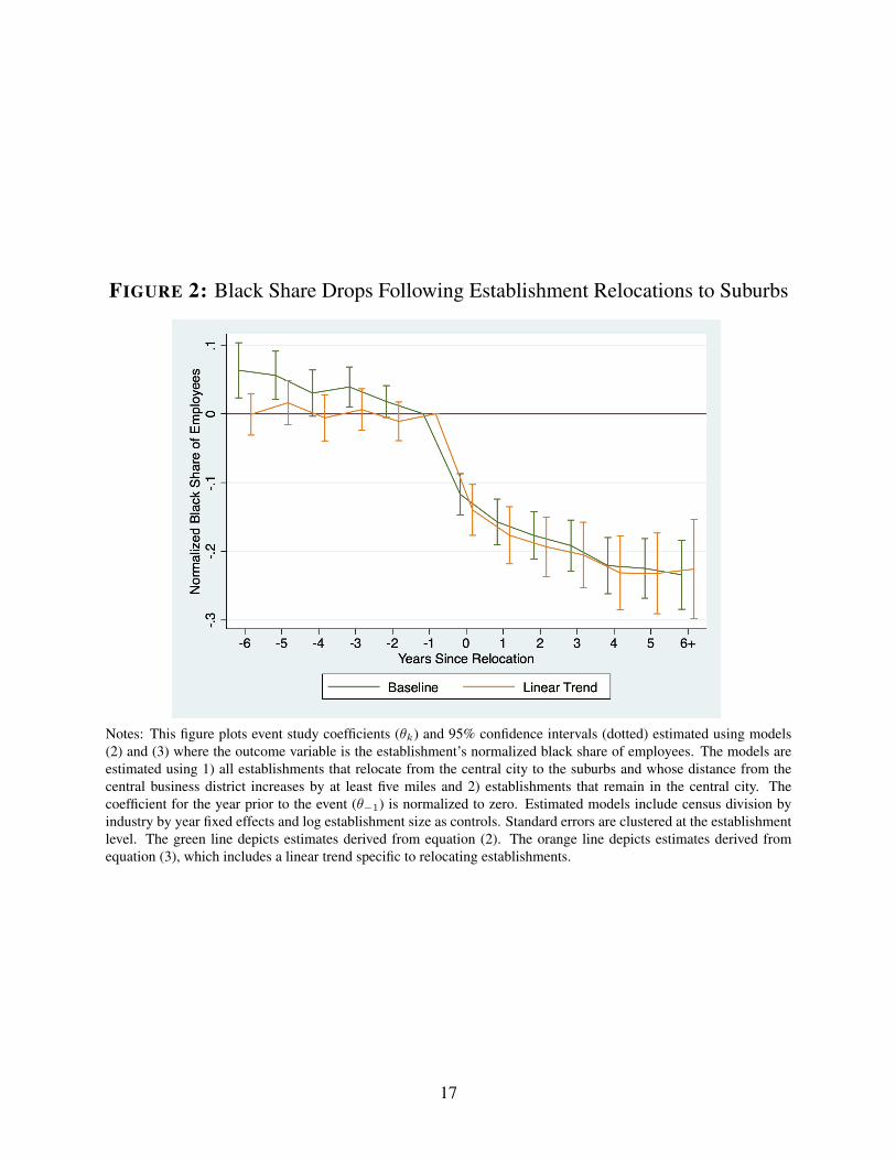
FIGURE 2: Black Share Drops Following Establishment Relocations to Suburbs

Notes: This figure plots event study coefficients (θk) and 95% confidence intervals (dotted) estimated using models(2) and (3) where the outcome variable is the establishment’s normalized black share of employees. The models areestimated using 1) all establishments that relocate from the central city to the suburbs and whose distance from thecentral business district increases by at least five miles and 2) establishments that remain in the central city. Thecoefficient for the year prior to the event (θ−1) is normalized to zero. Estimated models include census division byindustry by year fixed effects and log establishment size as controls. Standard errors are clustered at the establishmentlevel. The green line depicts estimates derived from equation (2). The orange line depicts estimates derived fromequation (3), which includes a linear trend specific to relocating establishments.

17

allows for a linear trend specific to relocating establishments. In particular, I estimate

(norm. black share)jt = αj+λd(j),i(j),t+δ(ever relocatej)×t+γ log(est. size)jt+b∑

k=a

θkDkjt+εjt,

(3)

where (ever relocate)j is an indicator for whether establishment j ever relocates from the central

city and (ever relocate)j × t is a differential time trend for relocating establishments. In this spec-

ification I adjust the definition of D−6jt , the endpoint lead for relocation, to D−6

jt = 1(t = τj − 6).

In words, I no longer pool six years prior to the relocation with earlier years so that D−6jt is now an

indicator for exactly six years prior to relocation.

Figure 2 presents the θ coefficients from this alternative specification. The θ coefficients are

now consistently near zero prior to relocation, yet the post-relocation θ coefficients are near iden-

tical to the corresponding estimates from the baseline model. Hence, I conclude that differential

pre-trends cannot account for the sharp drop in establishment black share following relocation,

either qualitatively or quantitatively.

In Online Appendix A, I also show that the change in the racial composition of employees at

relocating establishments is not driven by coincident changes in the occupational composition of

employees at those establishments. Black workers are substantially less likely to work the same

job following its relocation to the suburbs.

While an establishment’s drop in normalized black share following relocation is large, the aver-

age drop one would have predicted for these establishments using the cross-sectional relationship

between establishment location and normalized black share is about 50% larger at 0.35.20 This

discrepancy may reflect some combination of the following: (1) the causal effect of location is

heterogeneous, and relocating establishments are atypical21; (2) the β coefficients from equation

(1) are not the causal effect of establishment location; and (3) the effect of an establishment loca-20In particular, I estimate a variant of equation (1), allowing the β coefficient to vary by MSA, and then use the

estimated model to predict the normalized black share for all establishments in the data based on the MSA and distancefrom the CBD alone. I then calculate the average change in predicted normalized black share following relocation,averaging across relocating establishments.

21Note that relocating establishments have relatively low black shares even prior to relocation.

18

tion is not the same as the effect of an establishment relocation. The effects may not coincide if,

for example, central city residents are more aware of job opportunities at establishments that have

relocated to the suburbs than establishments that are already located in the suburbs. Nonetheless,

the effect of relocation is substantial. Given that, as documented in Section 4, the share of MSA

jobs located in the central city declines by 10% per decade from 1970 to 2000, the estimated causal

effect of establishment relocations suggests that job suburbanization will reduce the black share of

the workforce by about 2.3% each decade.

4 Job Suburbanization and Racial Inequality across Labor Mar-

kets

I have shown that conditional on job characteristics, black workers are less likely than white work-

ers to work in suburbs, and this segregation persists despite widespread job suburbanization over

time. This finding suggests that job suburbanization may reduce black labor market opportunities

and increase racial labor market inequality. However, suburbanization may be offset by worker

re-sorting across workplaces so that, at the market level, the effect of suburbanization on racial

inequality is muted. In this section, I exploit variation across MSAs to estimate the local labor

market-level relationship between job suburbanization and black employment rates and earnings

using census data.

In analyzing labor market outcomes, I restrict attention to men and women between the ages

of 24 and 63 who are non-Hispanic white or black. To measure employment, I use an indicator

for whether an individual is currently labor market “active,” meaning employed or in school.22

In practice, this measure reflects employment because only a small fraction of individuals in my

sample report being in school, and this does not differ significantly by race. For this reason, I use

“active” and “employed” interchangeably.

Combining data from each census, I construct a synthetic panel by collapsing individuals into

22The results are similar if I use weeks worked as the employment measure.

19

cells and merging cells across years. I group individuals by MSA of residence, gender, race,

education, and cohort. These groups are indexed by g. I exclude those who are institutionalized

because individuals in that population may not be residing in their relevant labor market. This may

attenuate the relevant estimates below given that incarceration rates began to increase substantially

in the mid-1970s and a large share of black adults was incarcerated, though the cohorts I focus on

will have largely “aged-out” of criminal activity by 1980 (Western and Pettit, 2000). Patterns for

women should be less susceptible to this issue given their relatively low incarceration rates. I divide

the sample into three education groups: less than high school graduate, high school graduate, and

college graduate. I also divide the sample into cohorts, those who are the following ages in 1970:

24–33, 34–43, and 44–53.23 I group by cohort rather than age because the intention is to follow

the same group of individuals from decade to decade.24 Of course, the composition of cells may

change from decade to decade due to migration; I explore the role migration plays in the analysis

in Online Appendix A. I restrict the analysis to cells with at least 25 observations and weight cells

by their size. This leaves 1,607 cells in 1970 over 58 MSAs.

Table 2 presents summary statistics on the demographics and labor market outcomes for the

synthetic cohorts. Black men are employed at lower rates than white men in 1970 and experience

larger proportional declines in employment in the short run and long run. By contrast, black women

are employed at higher rates than white women in 1970, though white women experience larger

increases in employment rates over time. From 1970 to 2000, the share of the black population

living in the central city declines by 22%, while the share of the white population living in the

central city declines by 31%. The share of MSA jobs located in the central city declines by 9%–

10% each decade.23This corresponds to individuals born in 1917–1926, 1927–1936, and 1937–1946.24Moreover, there are important changes in the educational opportunities children face over this period, and these

changes vary across MSAs and by race. In particular, following the Brown v. Board of Education Supreme Courtdecision of 1954, many large urban school districts were mandated to desegregate under federal court order. Thesecourt orders had substantial effects on school segregation and black educational attainment (Guryan, 2004). In addi-tion, while many black individuals in older cohorts residing outside of the South were educated in the South, this isless true for younger cohorts. Hence, even within a given MSA, educational experience across cohorts varies widely,particularly for black adults.

20

TABLE 2: Sample Descriptive Statistics, Cell Level

Black White1970 1980 1990 2000 1970 1980 1990 2000

Share 0.132 0.138 0.126 0.143 0.868 0.862 0.874 0.857

Female 0.563 0.565 0.574 0.576 0.515 0.517 0.517 0.518

1917-1926 0.287 0.285 — — 0.341 0.343 — —1927-1936 0.335 0.317 0.455 —- 0.313 0.310 0.478 —1937-1946 0.378 0.398 0.545 1.000 0.346 0.346 0.522 1.000

<HS Grad 0.559 0.487 0.410 0.329 0.289 0.241 0.173 0.125HS Grad 0.402 0.452 0.501 0.569 0.541 0.556 0.565 0.568College Grad 0.038 0.060 0.089 0.102 0.170 0.203 0.262 0.307

Active, Male 0.868 0.747 0.693 0.546 0.947 0.869 0.819 0.714(0.059) (0.121) (0.144) (0.113) (0.030) (0.106) (0.127) (0.090)

Active, Female 0.568 0.594 0.616 0.489 0.479 0.554 0.623 0.565(0.117) (0.155) (0.173) (0.123) (0.080) (0.122) (0.156) (0.100)

πcc 0.529 0.489 0.460 0.423 0.525 0.489 0.459 0.422(0.111) (0.125) (0.156) (0.169) (0.112) (0.120) (0.146) (0.160)

∆ log(πcc) — -0.094 -0.094 -0.110 — -0.089 -0.089 -0.107— (0.110) (0.137) (0.079) — (0.104) (0.126) (0.073)

Share Living in 0.795 0.734 0.678 0.617 0.393 0.324 0.292 0.270Central City (0.131) (0.155) (0.181) (0.207) (0.157) (0.150) (0.153) (0.155)

Notes: This table includes 58 consistently identified MSAs with the largest black populations in 1970 and onlycells with at least 25 individuals. Statistics are weighted by cell size. See Section 4 for further details on cellconstruction. “Active” refers to the share of a cell employed or in school. πcc refers to the fraction of MSA jobslocated in the central city. “Share Living in Central City” refers to the share of an entire racial group living inthe central city of each cell’s MSA, not the share of cell living in the central city. The latter cannot be identifiedin all years of the census data.

21

4.1 Empirical Strategy

I test the spatial mismatch hypothesis by estimating the relationship between job suburbanization

and black-white inequality in employment rates and earnings, exploiting variation across MSAs. In

particular, I test whether black cohorts experience larger declines in employment rates and earnings

relative to comparable white cohorts in MSAs that experience more job suburbanization. I estimate

linear differences-in-differences models of the form

∆Ymg =αg + β∆ log(πccm) + f(Y t0mg)γ

+ blackg ×(βB∆ log(πccm) + f(Y t0

mg)γB)

+ εmg,

(4)

where g indexes groups, m indexes markets, αg are group fixed effects, and blackg is an indicator

for a cell of black individuals. Yg is either the log employment rate or log average annual earnings

corresponding to a cell g.25 In some specifications I do not condition on baseline employment

rates (earnings), but in others I specify f(·) as a quadratic function. I include a control for a

polynomial in baseline Y because employment or earnings growth may depend nonlinearly on

baseline employment or earnings.26 In some specifications I include MSA-by-education category

fixed effects (and omit the collinear ∆ log(πccm) term) to isolate within-skill group racial differences

in outcomes. The coefficient β has the following elasticity interpretation: a 1% decline in the

fraction of MSA jobs located in the central city is associated with a β% decline in cell employment.

The coefficient βB reflects the relative decline for black cells. I cluster standard errors at the MSA

level.

Before describing the baseline results, I explore how job suburbanization relates to other base-

line cell-level and MSA-level characteristics. One concern with the empirical strategy described

here is that job suburbanization may occur in areas where employment is already declining, partic-

ularly for black workers. Though the 1960 census does not identify MSAs, for half the respondents

in the 1970 census, I can observe their employment status in 1965. To measure pre-trends by cell,

25The results are similar if I use the employment rate rather than log employment rate as the outcome of interest.26For example, because the cell employment rate is capped at 1, cells with high baseline employment rates have

very little potential for growth relative to cells with lower baseline employment.

22

I use the change in employment rates by cell, assigning individuals to MSAs using their residence

in 1970. I estimate models of the form

∆PRE log (Emp. Rate)mg = αg + β∆ log(πccm) + βBblackg × ∆ log(πccm) + εmg. (5)

I estimate separate models for job suburbanization occurring over the short run (1970 to 1980) and

long run (1970 to 2000). Table 3, Panel A provides the results. I find that cells that experienced

more job suburbanization from 1970 to 1980 had somewhat lower employment growth from 1965

to 1970. For suburbanization occurring from 1970 to 2000, the magnitude is even smaller and

statistically insignificant. Importantly, the differences in trends between black and white cells is

statistically insignificant in both cases and have opposite signs. Hence, black employment does

not appear to be on a differential trend in suburbanizing MSAs.

A second concern is that job suburbanization is associated with other covariates that may in-

fluence labor market outcomes differently for black and white workers. Table 3, Panel B provides

coefficient estimates for models in the form

∆ log(πccm) = αg +Wmgδ + blackg ×WmgδB + εmg, (6)

where Wm is a vector of cell-level and MSA-level covariates. I relate these correlates to short

run and long run subsequent job suburbanization. I relate job suburbanization to the following

baseline cell-level characteristics: log employment rate active, log average earnings. I also include

the following baseline MSA-level characteristics: fraction of jobs in the central city, black share

of population, racial residential segregation, violent crime rate, and property crime rate. To mea-

sure residential segregation I use the dissimilarity index constructed in Cutler et al. (1999). Data

on reported crimes come from the FBI’s Uniform Crime Reports. The UCR reports crimes per

100,000 for seven types of offenses: murder, rape, robbery, aggravated assault, burglary, larceny,

and motor vehicle theft. I divide these seven offenses into two categories, violent and property

crimes, and sum within these categories. I standardize the MSA-level covariates to have mean zero

23

TABLE 3: Job Suburbanization and Baseline Cell and MSA Characteristics

Panel A: Employment (1965 to 1970) 1970-1980 1970-2000Outcome: ∆PRE log (Emp. Rate)

∆ log(πcc) 0.083˜ 0.034(0.049) (0.060)

∆ log(πcc) × black 0.058 -0.040(0.040) (0.027)

Group FEs Yes YesN Cells 1607 563N MSAs 58 58

Panel B: 1970 Characteristics 1970-1980 1970-2000Outcome: ∆ log(πcc) δ δB δ δB

Log Fraction Active (Group) 0.318˜ -0.018 0.246 -0.088(0.160) (0.095) (0.300) (0.209)

Log Earnings (Group) -0.168 -0.056 -0.045 -0.281(0.098) (0.071) (0.229) (0.196)

Fraction of Work in Central City (MSA), -0.008 -0.002 0.072* 0.019Standardized (0.017) (0.010) (0.031) (0.021)Fraction Black (MSA), -0.022 -0.020 -0.114** -0.058˜Standardized (0.019) (0.014) (0.039) (0.033)Dissimilarity Index (MSA), -0.036** -0.009 -0.098** -0.016Standardized (0.012) (0.011) (0.026) (0.018)Violent Crime Rate (MSA), -0.004 0.012 0.110 0.011Standardized (0.019) (0.011) (0.052) (0.026)Property Crime Rate (MSA), -0.005 -0.003 -0.089* 0.006Standardized (0.017) (0.012) (0.036) (0.025)

Group FEs Yes YesN Cells 1564 547N MSAs 56 56

Notes: Panel A displays estimates of equation (5). In Panel A, the outcome is cell-level changes in em-ployment rates from 1965 to 1970. Panel B displays estimates of equation (6). In this panel, the outcomeis MSA job centralization. Columns (1) and (2) refer to centralization from 1970 to 1980; columns (3) and(4) refer to centralization from 1970 to 2000. The odd columns display the estimated δ coefficients fromequation (6), the “main effects”; the even columns display the estimated δB coefficients, the black cellinteractions. All models include group fixed effects (fixed effects for all combinations of cohort, education,sex, and race). Dissimilarity segregation indices are taken from Cutler et al. (1999). Standard errors are inparentheses, clustered at the MSA level. Regression models are weighted by cell size. ˜ Denotes statisticalsignificance at the p < 0.10 level. * Denotes statistical significance at the p < 0.05 level. ** Denotesstatistical significance at the p < 0.01 level.

24

and standard deviation of one across MSAs.

From 1970 to 1980, I find residential segregation to be a significant predictor of job subur-

banization across cells. Baseline employment rates are a marginal predictor. Notably, these re-

lationships do not differ significantly for black cells. From 1970 to 2000, baseline residential

segregation and the black share of the population are significant predictors of job suburbanization.

This is consistent with research suggesting that black in-migration to central cities was a major

cause of “white flight” (Boustan, 2010). The baseline fraction of jobs located in the central city is

a marginal predictor.

4.2 Baseline Estimates

I estimate variants of equation (4) for three periods: 1970 to 1980, 1970 to 1990, and 1970 to 2000.

Table 4 provides these baseline estimates. In the top panel, the outcome is log employment rate.

In the bottom panel, the outcome is log average earnings. In columns (1)–(3) the period is 1970

to 1980, in columns (4)–(6) the period is 1970–1990, and in columns (7)–(9) the period is 1970

to 2000. All columns include group fixed effects. All columns except (1), (4), and (7) include

controls for a quadratic in baseline employment rates or log average earnings interacted with race.

Columns (3), (6), and (9) include MSA-by-education fixed effects.

Across specifications and periods, changes in the spatial distribution of work have little as-

sociation with white employment rates. The coefficient is generally small in magnitude and is

statistically indistinguishable from zero at the 10% level. By contrast, job suburbanization is asso-

ciated with declines in black employment, and the relationship is statistically significant at the 1%

level across specifications. I first focus on specifications that do not include MSA-by-education

fixed effects (all but columns (3), (6), and (9)). Over the 1970s, the βB coefficient of 0.25 to

0.29 implies that a 10% decline in the fraction of MSA jobs located in the central city—about the

mean level experienced over this period—is associated with a 2.5% to 2.9% decline in the black

employment rate, relative to the white employment rate. The estimates for annual earnings have

the same sign, but the coefficients are more dependent on the inclusion of baseline earnings and

25

TAB

LE

4:Jo

bSu

burb

aniz

atio

nan

dL

abor

Mar

ketO

utco

mes

1970

-198

019

70-1

990

1970

-200

0

Out

com

e:∆

log

(Em

p.R

ate)

(1)

(2)

(3)

(4)

(5)

(6)

(7)

(8)

(9)

∆lo

g(π

cc)

-0.0

30-0

.020

-0.0

23-0

.006

-0.0

39-0

.029

(0.0

51)

(0.0

57)

(0.0

71)

(0.0

49)

(0.0

48)

(0.0

37)

∆lo

g(π

cc)×

blac

k0.

247*

*0.

286*

*0.

229*

*0.

233*

*0.

181*

*0.

141*

*0.

232*

*0.

163*

*0.

121*

*(0

.065

)(0

.075

)(0

.057

)(0

.054

)(0

.057

)(0

.051

)(0

.041

)(0

.038

)(0

.044

)

Out

com

e:∆

log

(Avg

.Ear

ning

s)

∆lo

g(π

cc)

-0.0

30-0

.050

0.08

00.

093

0.02

70.

036

(0.0

66)

(0.0

75)

(0.1

01)

(0.1

05)

(0.0

62)

(0.0

66)

∆lo

g(π

cc)×

blac

k0.

365*

*0.

160

0.14

0˜0.

230*

0.14

30.

016

0.23

3**

0.12

4*0.

030

(0.0

97)

(0.0

94)

(0.0

80)

(0.0

76)

(0.0

79)

(0.0

73)

(0.0

72)

(0.0

57)

(0.0

57)

Gro

upFE

sY

esY

esY

esY

esY

esY

esY

esY

esY

esM

SA×

Edu

catio

nFE

sN

oN

oY

esN

oN

oY

esN

oN

oY

esB

asel

ine

Con

trol

sN

oY

esY

esN

oY

esY

esN

oY

esY

esN

Cel

ls16

0716

0716

0710

9910

9910

9956

356

356

3N

MSA

s58

5858

5858

5858

5858

Not

es:

The

tabl

edi

spla

yses

timat

esof

equa

tion

(4).

Col

umns

(1)–

(3)

refe

rto

mod

els

cove

ring

1970

–198

0,co

lum

ns(4

)–(6

)re

fer

tom

odel

sco

veri

ng19

70–1

990,

and

colu

mns

(7)–

(9)

refe

rto

mod

els

cove

ring

1970

–200

0.A

llm

odel

sin

clud

egr

oup

fixed

effe

cts

(fixe

def

fect

sfo

ral

lco

mbi

natio

nsof

coho

rt,e

duca

tion,

sex,

and

race

).C

olum

ns(2

),(3

),(5

),(6

),(8

),an

d(9

)in

clud

ea

quad

ratic

inlo

gba

selin

eem

ploy

men

trat

es(P

anel

A)

orlo

gav

erag

eea

rnin

gs(P

anel

B)i

nter

acte

dw

ithra

ce.C

olum

ns(3

),(6

),an

d(9

)inc

lude

MSA

-by-

educ

atio

nca

tego

ryfix

edef

fect

s.In

Pane

lA,t

heou

tcom

eis

chan

ges

inlo

gem

ploy

men

trat

es;i

nPa

nelB

,the

outc

ome

isch

ange

sin

log

aver

age

earn

ings

.A

llm

odel

sar

ees

timat

edat

the

cell

leve

l.St

anda

rder

rors

are

inpa

rent

hese

s,cl

uste

red

atth

eM

SAle

vel.

Reg

ress

ion

mod

els

are

wei

ghte

dby

cell

size

.˜D

enot

esst

atis

tical

sign

ifica

nce

atth

ep<

0.10

leve

l.*

Den

otes

stat

istic

alsi

gnifi

canc

eat

thep<

0.05

leve

l.**

Den

otes

stat

istic

alsi

gnifi

canc

eat

thep<

0.01

leve

l.

26

MSA-by-education fixed effects as controls.

From 1970 to 1990, a 10% decline in the fraction of jobs located in the central city is associated

with a 1.8% to 2.3% decrease in black relative employment. Over the full period, a 10% decline in

the fraction of jobs located in the central city is associated with a 1.6% to 2.3% decrease in black

relative employment. The latter relationship is estimated using a single cohort of workers: those

who were ages 24–33 in 1970 and 54–63 in 2000. Figure 3 displays this relationship graphically,

plotting ∆m log(πcc) against changes in log black and white employment rates for all individuals

in these cohorts pooled by MSAs. For black workers, there is a clear, positive relationship; for

white workers, there is no clear relationship.

A potential explanation for the negative relationship between job suburbanization and black

labor market outcomes is that it reflects racial differences in skill. Columns (3), (6), and (9)

include MSA-by-education fixed effects so that βB is identified by within-skill group variation.

βB decreases slightly in magnitude with the inclusion of these fixed effects, but the differences are

not statistically significant. The relationship between job suburbanization and racial labor market

inequality is a within-skill group phenomenon.

In Online Appendix Table A4, I examine heterogeneity in the baseline estimates by education

and gender. I focus on the 1970–2000 long difference. All models include a quadratic in baseline

employment or earnings. For employment, the βB coefficient is largest for high school dropouts

but is also present for high school and college graduates. The coefficient is somewhat larger for

women than men, though the difference is not statistically significant. This is striking given that

men and women tend to work in very different industries and occupations over this period. For

earnings, the relationship is present for women but not men.

Given that the average value for ∆ log(πcc) is about –0.1 for each decade, the observed job sub-

urbanization predicts a 1.6% to 2.3% relative decrease in black employment rates. This decrease is

comparable in magnitude to the decline in black share of the workforce implied by the establish-

ment relocation event study estimates as described in Section 3, and it suggests that the re-sorting

of black workers across workplaces did not significantly offset the effects of job suburbanization.

27

FIGURE 3: Job Suburbanization and Changes in Employment Rates, 1970–2000

(A) Synthetic Panel, BlackSlope = 0.172

Slope = 0.172

Slope = 0.172(0.042)

(0.042)

(0.042)-.6

-.6

-.6-.4

-.4

-.4-.2

-.2

-.20

0

0Change in Log(Black Employment Rate)

Chan

ge in

Log

(Bla

ck E

mpl

oym

ent

Rate

)

Change in Log(Black Employment Rate)-.8

-.8

-.8-.6

-.6

-.6-.4

-.4

-.4-.2

-.2

-.20

0

0.2

.2

.2Change in Log(Fraction of MSA Jobs in Central City)

Change in Log(Fraction of MSA Jobs in Central City)

Change in Log(Fraction of MSA Jobs in Central City)

(B) Synthetic Panel, WhiteSlope = - 0.012

Slope = - 0.012

Slope = - 0.012(0.035)

(0.035)

(0.035)-.3

-.3

-.3-.2

-.2

-.2-.1

-.1

-.10

0

0Change in Log(White Employment Rate)

Chan

ge in

Log

(Whi

te E

mpl

oym

ent

Rate

)

Change in Log(White Employment Rate)-.8

-.8

-.8-.6

-.6

-.6-.4

-.4

-.4-.2

-.2

-.20

0

0.2

.2

.2Change in Log(Fraction of MSA Jobs in Central City)

Change in Log(Fraction of MSA Jobs in Central City)

Change in Log(Fraction of MSA Jobs in Central City)

Notes: This figure plots changes in black and white employment rates against job centralization across 58 MSAs from1970 to 2000 for those born between 1937 and 1946 (ages 24—33 in 1970 and 54-63 in 2000). See Section 4.2 fordetails on the construction of synthetic cohorts.

28

To put this magnitude in perspective, note that from 1970 to 2000, the proportion of black men

ages 24–63 living in the MSAs analyzed here that were employed or in school decreased from 85

percentage points (p.p.) to 72 p.p. For white men, the proportion decreased from 92 p.p. to 87

p.p. Among women, the proportion employed or in school increased from 56 p.p. to 68 p.p. for

black women and from 47 p.p. to 73 p.p. for white women. Hence, the employment rate for black

men declined by about 10% more than the employment rate for white men, and the employment

rate for white women increased by about 34% more than the employment rate for black women.

βB estimates imply that job suburbanization can explain about 50%–70% of the relative decline in

black men’s employment rates and 15–20% of the relative increase in white women’s employment

rates.

The evidence presented in Table 4 and Figure 3 suggests that job suburbanization caused sub-

stantial declines in black employment rates relative to white employment rates. However, there

are three reasons to be cautious in assigning a causal interpretation. First, job suburbanization

may be an endogenous response to unobserved, racially distinct labor supply shocks. In particular,

job suburbanization may be concentrated in markets where black workers become relatively less

productive so that black employment rates would have declined in those markets even if jobs had

not moved to the suburbs. Second, suburbanization may be related to other changes in the local

industry or occupation mix that would have otherwise portend reductions in black relative employ-

ment rates. Third, job suburbanization may be associated with migration patterns in a way that

contaminates the synthetic panel design. I address each of these concerns below.

4.3 Highways as a Source of Variation

Unobserved shocks to the productivity of black workers could induce firms to migrate and produce

black employment declines, even in the absence of a spatial mismatch mechanism. For example,

the emergence of crack cocaine markets in the 1980s and 1990s could potentially explain both the

deterioration of black labor supply and the relocation of employers from the central city (Evans et

al., 2016).

29

To test whether the observed relationship between job suburbanization and declines in black

relative employment is driven entirely by such productivity shocks, I require an instrument for job

suburbanization that is plausibly orthogonal to such shocks. More generally, the ideal instrument

would satisfy an exclusion restriction: it would only (potentially) affect black employment by

changing the spatial distribution of work.

To instrument for job suburbanization, I exploit a previously used source of variation in sub-

urbanization: the interstate highway system (Baum-Snow, 2007; Michaels, 2008). Highways can

potentially increase suburbanization through several mechanisms. First, they decrease transporta-

tion costs for both firms and households. For firms, highways make physical proximity to other

transportation hubs (e.g., ports and rail stations) and upstream or downstream firms less important,

allowing them to take advantage of cheaper land and other suburban amenities. Michaels (2008)

argues that as highway construction was nearing completion, trucks became the primary mode of

shipping goods within the United States. For households, highways reduce the costs of commut-

ing to central work and access to other central city amenities from a suburban residence. These

direct effects on transportation costs may also have feedback effects. By increasing the number

of firms and households in the suburbs, they make these areas more attractive for other firms and

households. Firms may then follow workers moving to the suburbs and achieve agglomeration

economies there.

Baum-Snow (2007) documents that the U.S. interstate highway system played an important

role in post-war residential suburbanization. With nearly all construction occurring between 1956

and 1980, the interstate highway system would ultimately span over 40,000 miles. The highway

system was originally designed to connect major metropolitan areas, serve U.S. national defense,

and connect major routes in Canada and Mexico. Using plausibly exogenous variation in highway

construction across MSAs, Baum-Snow (2007) finds that one new highway passing through a cen-

tral city reduces its population from 1950 to 1990 by about 18%. These effects are substantial: they

imply that the interstate highway system accounts for about one-third of the decline in central city

population relative to total MSA growth over this period. Using a similar identification strategy,

30

Baum-Snow (forthcoming) finds that highways also caused substantial job suburbanization.

Highways are an imperfect instrument for job suburbanization: research has documented that

highways have a variety of effects on the labor market, and it is possible that they affect black

relative employment through channels other than the spatial distribution of work.27 However, in

Online Appendix A I provide evidence that highways do not appear to affect labor demand for

worker skills in a way that would disproportionately affect black workers.

Highways also affect residential neighborhoods. In Online Appendix A I show that, in the

sample of MSAs examined here, highway rays predict the suburbanization of white households at

a magnitude consistent with Baum-Snow (2007) but not the location of black households. This

disparity is consistent with a central premise of the spatial mismatch hypothesis: black households

faced significant additional barriers to suburban residence over this period. Accordingly, highway

rays also increase subsequent segregation, with each ray predicting a 0.01, 0.045, and 0.053 unit

increase in a city’s dissimilarity index by 1980, 1990, and 2000.

Building the interstate highway system also forced the destruction of neighborhoods and dis-

placement of households, particularly in central cities. There is evidence that black households

faced a disproportionate share of displacements and that local planners exploited interstate con-

struction as an opportunity to eliminate poor, “blighted,” and often black communities (Rose and

Mohl, 2012). This suggests another channel through which the interstate highways system may

affect black relative employment rates, potentially violating the exclusion restriction. However,

more than 90% of interstate-central city intersections in the MSAs I study were already built by

1970. Hence, the effects of neighborhood clearances would likely already be reflected in baseline

labor market outcomes. For the analysis below, my measure of MSA highway exposure is the

stock of interstate highway rays emanating from the central city in 1970.

27Michaels (2008) finds that highways increased trade for exposed rural counties and raised the relative demandfor skilled manufacturing workers in skill-abundant rural counties while reducing it elsewhere. Duranton et al. (2014)find that highways lead cities to increase the weight of their exports and specialize in sectors producing heavy goods.Duraton and Turner (2012) find that interstate highways increased MSA growth from 1983 to 2003.

31

4.3.1 Are Highways Endogenous to Labor Supply Shocks?

A potential concern with exploiting variation derived from the interstate highway system is that

highway assignment may be determined endogenously. As Baum-Snow (2007) notes, the interstate

highway system was likely in part designed to facilitate local commuting and local economic

development in particular regions. Though less plausible, the highway system might have also

been designed accounting for productivity shocks particular to black workers in the 1970s. To deal

with this, I instrument for realized highway construction using the 1947 federal interstate highway

plan as in Baum-Snow (2007).

In 1937, the Franklin D. Roosevelt administration began to plan an interstate highway system.

In their recommended highway plan, the National Interregional Highway Committee considered

the distribution of population, manufacturing activity, agricultural production, the location of post-

World War II employment, a strategic highway network drawn up by the War Department in 1941,

military and naval establishment locations, and interregional traffic demand, in that order. This

led to the Federal Highway Act of 1944, which instructed the roads commissioner to develop an

initial plan for a national interstate highway system. As specified by the legislation, the highways

in the planned system were to be “so located as to connect by routes as direct as practicable, the

principal metropolitan areas, cities, and industrial centers, to serve the national defense, and to

connect at suitable border points with routes of continental importance in the Dominion of Canada

and the Republic of Mexico...” (as cited in Baum-Snow, 2007). Importantly, the legislation makes

no mention of local commuting or local economic development. The final plan produced under

this act, approved in 1947, is presented in Online Appendix Figure A2.

Major funding for the interstate highway system began with the Federal Aid Highway Act of

1956. The 1956 Federal Aid Highway Act expanded the 1947 plan and committed the federal gov-

ernment to pay 90% of the cost of construction. In particular, the 1956 plan incorporated additional

highways that were designed for local purposes like commuting and development. Therefore, in

some specifications I instrument for actual highway rays using highway rays planned in 1947. The

first-stage t-statistic is in excess of 5.

32

4.3.2 Empirical Strategy and Results

I explore the relationship between highways, job suburbanization, and employment rates by race.

In all subsequent analyses, my measure of highway exposure is the number of interstate highway

rays emanating from the central city in 1970. I estimate specifications of the form

∆Ymg =αg + γ1rays1970m + γ2radiusm + f(emp1970)mg +Xmγ3

+ blackg ×(γB1 rays

1970m + γB2 radiusm + +Xmγ

B3

)+ εmg,

(7)

where rays1970m denotes the number highway rays emanating from the central city of MSA m

in 1970 and radiusm is the radius of the central city, a key control in the analysis of Baum-

Snow (2007). Intuitively, one must control for the central city radius because it determines the

extent to which sprawl is reflected in suburbanization measures, and highways are more likely to

travel through central cities that are physically larger. Note that the average number of central city

highway rays in 1970, weighted by the sample population size, is 3.9; the unweighted average is

3.28

As in Table 3, I begin by relating highways to pre-period changes in employment rates and

baseline cell and MSA characteristics. The results are presented in Online Appendix Table A5.

There is no relationship between an MSA’s highway stock in 1970 and cell-level changes in em-

ployment rates from 1965 to 1970. Notably, highway assignment has little relationship with an

MSA’s racial composition in 1970. Similarly, Baum-Snow (2007) finds that planned and actual

highway construction has little relationship with an MSA’s racial composition in 1950.

Table 5, Panel A presents estimates of equation (7) where the outcome is ∆m log(πcc). I find

that the stock of highways in 1970 predicts job suburbanization thereafter. In odd specifications

I use actual interstate highway rays constructed as the explanatory variable of interest; in even

specifications I instrument for highways constructed using highway rays included in the 1947 plan.

In all columns, t0 is 1970, while t1 is 1980 in columns (1) and (2), 1990 in columns (4) and (5),

and 2000 in columns (7) and (8). In the baseline OLS specification, one highway ray emanating28Note that if a highway passes through a central city, this counts as two rays.

33

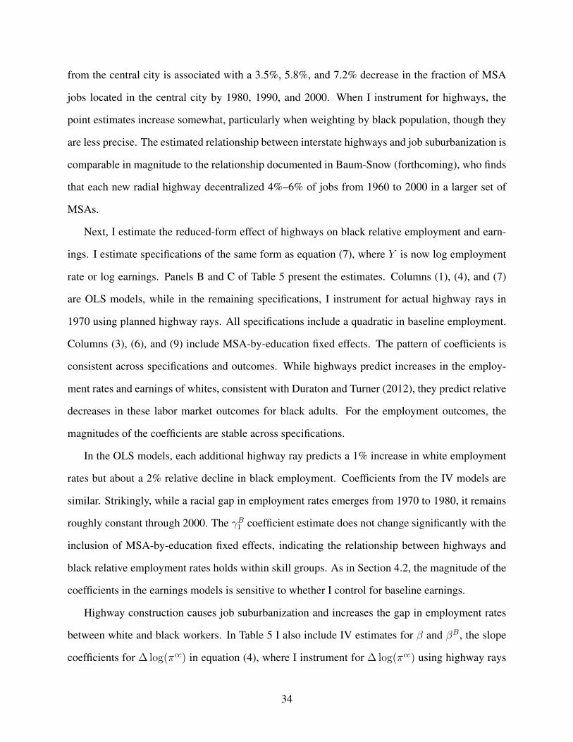
from the central city is associated with a 3.5%, 5.8%, and 7.2% decrease in the fraction of MSA

jobs located in the central city by 1980, 1990, and 2000. When I instrument for highways, the

point estimates increase somewhat, particularly when weighting by black population, though they

are less precise. The estimated relationship between interstate highways and job suburbanization is

comparable in magnitude to the relationship documented in Baum-Snow (forthcoming), who finds

that each new radial highway decentralized 4%–6% of jobs from 1960 to 2000 in a larger set of

MSAs.

Next, I estimate the reduced-form effect of highways on black relative employment and earn-

ings. I estimate specifications of the same form as equation (7), where Y is now log employment

rate or log earnings. Panels B and C of Table 5 present the estimates. Columns (1), (4), and (7)

are OLS models, while in the remaining specifications, I instrument for actual highway rays in

1970 using planned highway rays. All specifications include a quadratic in baseline employment.

Columns (3), (6), and (9) include MSA-by-education fixed effects. The pattern of coefficients is

consistent across specifications and outcomes. While highways predict increases in the employ-

ment rates and earnings of whites, consistent with Duraton and Turner (2012), they predict relative

decreases in these labor market outcomes for black adults. For the employment outcomes, the

magnitudes of the coefficients are stable across specifications.

In the OLS models, each additional highway ray predicts a 1% increase in white employment

rates but about a 2% relative decline in black employment. Coefficients from the IV models are

similar. Strikingly, while a racial gap in employment rates emerges from 1970 to 1980, it remains

roughly constant through 2000. The γB1 coefficient estimate does not change significantly with the

inclusion of MSA-by-education fixed effects, indicating the relationship between highways and

black relative employment rates holds within skill groups. As in Section 4.2, the magnitude of the

coefficients in the earnings models is sensitive to whether I control for baseline earnings.

Highway construction causes job suburbanization and increases the gap in employment rates

between white and black workers. In Table 5 I also include IV estimates for β and βB, the slope

coefficients for ∆ log(πcc) in equation (4), where I instrument for ∆ log(πcc) using highway rays

34

TABLE 5: Highways, Job Suburbanization, and Labor Market Outcomes

1970-1980 1970-1990 1970-2000

OLS IV IV OLS IV IV OLS IV IVOutcome: ∆ log(πcc) (1) (2) (3) (4) (5) (6) (7) (8) (9)

Rays1970 -0.035** -0.037* -0.058** -0.079** -0.072** -0.110**(0.010) (0.017) (0.015) (0.024) (0.020) (0.030)

Rays1970 × black -0.005 -0.016 -0.005 -0.024 -0.007 -0.027(0.006) (0.009) (0.007) (0.013) (0.009) (0.018)

Outcome: ∆ log (Emp. Rate)

Rays1970 0.008* 0.0110* 0.009* 0.015* 0.012** 0.020*(0.004) (0.005) (0.004) (0.006) (0.004) (0.008)

Rays1970 -0.022** -0.021* -0.015* -0.018* -0.018 -0.012 -0.019** -0.028** -0.021**× black (0.005) (0.009) (0.007) (0.007) (0.011) (0.009) (0.007) (0.010) (0.008)

β, IV -0.235˜ -0.295 -0.156˜ -0.188˜ -0.156˜ -0.180˜(0.132) (0.229) (0.079) (0.106) (0.80) (0.096)

βB , IV 0.575** 0.486* 0.288* 0.220* 0.249** 0.242**(0.198) (0.224) (0.121) (0.105) (0.094) (0.087)

Outcome: ∆ log (Earnings)

Rays1970 0.009˜ 0.021** 0.011 0.006 0.021* 0.015(0.005) (0.007) (0.007) (0.012) (0.010) (0.014)

Rays1970 -0.020** -0.022* -0.021* -0.020 -0.015 0.003 -0.016 -0.022 -0.008× black (0.006) (0.011) (0.009) (0.011) (0.015) (0.013) (0.011) (0.018) (0.012)

β, IV -0.285 -0.616 -0.192 -0.074 -0.222˜ -0.143(0.195) (0.394) (0.147) (0.166) (0.127) (0.150)

βB , IV 0.586** 0.630 0.364 0.172 0.239 0.192(0.221) (0.393) (0.233) (0.172) (0.173) (0.150)

Group FEs Yes Yes Yes Yes Yes Yes Yes Yes YesMSA × Education FEs No No Yes No No Yes No No YesBaseline Controls Yes Yes Yes Yes Yes Yes Yes Yes YesCC Radius Control Yes Yes Yes Yes Yes Yes Yes Yes YesN Cells 1559 1559 1559 1066 1066 1066 545 545 545N MSAs 56 56 56 56 56 56 56 56 56

Notes: The table displays estimates of equation (7). Columns (1)–(3) refer to models covering 1970–1980, columns (4)–(6) refer to modelscovering 1970–1990, and columns (7)–(9) refer to models covering 1970–2000. In columns (2), (3), (5), (6), (8), and (9), actual highwayrays in 1970 are instrumented with planned highways. All models include group fixed effects (fixed effects for all combinations of cohort,education, sex, and race), a quadratic in log baseline employment (Panels A and B) or log average earnings (Panel C) interacted with race,and central city radius interacted with race. Columns (3), (6), and (9) include MSA-by-education fixed effects. In Panel A, the outcome ischanges in log fraction of MSA jobs located in the central city; in Panel B, the outcome is changes in log employment rates; in Panel C, theoutcome is changes in log earnings. “β, IV” and “βB , IV” are the implied IV estimates for β and βB , where highway rays or planned raysare instrumented for ∆ log(πcc). All models are estimated at the cell level. Two MSAs are not included in the highway data (Baum-Snow,2007): Jackson, MS and West Palm Beach, FL. Standard errors are in parentheses, clustered at the MSA level. Regression models areweighted by cell size. ˜ Denotes statistical significance at the p < 0.10 level. * Denotes statistical significance at the p < 0.05 level. **Denotes statistical significance at the p < 0.01 level.

35

or planned rays.29 In specifications corresponding to columns (1), (3), (5), and (6), the first-stage

(Panel A of Table 5) Angrist-Pischke F-statistics exceed 10, allaying concerns over weak identifi-

cation in these models (Angrist and Pischke, 2009).30 Columns (5) and (6) indicate that for every

10% decrease in the fraction of jobs located in the central city induced by highways from 1970 to

2000, black employment rates decline by 2.4% to 2.5% relative to white employment rates. While

job suburbanization might not be the only mechanism through which highways affect relative em-

ployment rates, labor supply shocks are unlikely to be an alternative, and changes in labor demand

are also unlikely to be a significant channel. Yet the relationship between job suburbanization

and black employment implied here is comparable to the baseline estimates from Section 4.2,31

corroborating a causal interpretation of the relationship between job suburbanization and black

employment.

4.4 Additional Robustness Checks

In Online Appendix A, I consider and rule out two alternative interpretations for the relationship

between job suburbanization and black-white differences in employment rates documented above.

First, I explore whether job suburbanization, including interstate highway-induced suburbaniza-

tion, is associated with changes in the types of work performed in the labor market. Specifically, I

test whether MSAs that experience greater job suburbanization also experience relative growth in

industries or occupations that disproportionately employed white workers in 1970. I conclude that

the causal effect of interstate highways on racial differences in employment rates is not driven by

changes in sector composition.

Second, I test whether the relationship between job suburbanization and black-white differ-

ences in employment rates is driven by the endogenous migration of households. Due to data

29More specifically, I estimate variants of equation (7) where I replace rays1970m with ∆ log(πcc) and instrument for∆ log(πcc

m) and blackg × ∆ log(πccm) using rays1970m and blackg × rays1970m . β and βB correspond to the coefficients

on ∆ log(πccm) and blackg × ∆ log(πcc

m).30In the specification corresponding to column (4), the Angrist-Pischke F-statistics associated with Rays1970 and

Rays1970× black are 8.63 and 13.2. In the specification corresponding to column (2), both are below 10.31The IV estimates are generally larger in magnitude but also less precise, and so they are statistically indistinguish-

able from baseline estimates.

36

limitations, I conduct the main analysis using a synthetic panel rather than a true panel of individ-

uals. For the same reason that residential sorting is a concern for any cross-sectional analysis, the

endogenous migration of households to and from MSAs may introduce a compositional bias in the

synthetic panel analysis. The productivity of migrants to and from an MSA may vary systemat-

ically with job suburbanization so that the correlation between job suburbanization and employ-

ment rate changes may in part reflect the changing composition of cells rather than within-person

changes. Using true panel of individuals from 1975 to 1980, I find that endogenous migration is

not a first order concern and the relationship between job suburbanization and racial differences in

employment rates are similar whether I use a true panel or a synthetic panel.

5 Mechanisms of Spatial Mismatch

This paper shows that, consistent with the spatial mismatch hypothesis, relocating a job to the sub-

urbs reduces the likelihood that the worker holding that job is black, and that job suburbanization

reduced black employment rates from 1970 to 2000. These findings raise a natural question: why?

For example, why don’t black workers follow jobs to the suburbs? And why don’t more firms

locate in the central city to employ displaced black workers? While a complete exploration of the

mechanisms that generate a link between job suburbanization and racial inequality in the labor

market is beyond the scope of this paper, this section summarizes potential mechanisms and the

necessary ingredients for the spatial mismatch hypothesis to hold.

The spatial mismatch hypothesis predicts that the suburbanization of work reduces black rel-

ative employment via spatial frictions in the labor and housing markets. Coulson et al. (2001)

develop a general equilibrium spatial search model that identifies the conditions necessary to gen-

erate higher unemployment rates in the central city due to spatial frictions. The model can be easily

adapted to identify the conditions under which job suburbanization reduces black employment.

In the Coulson et al. (2001) framework, the following conditions are sufficient for spatial mis-

match to emerge in equilibrium (Johnson, 2006):

37

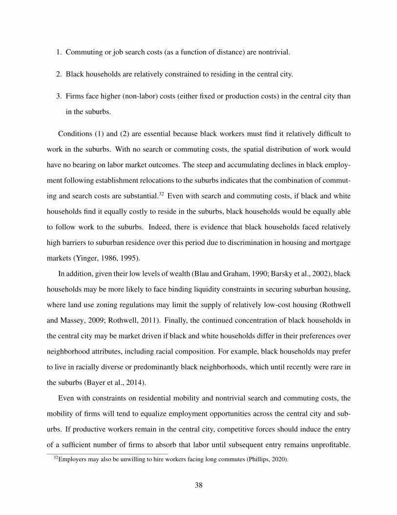
1. Commuting or job search costs (as a function of distance) are nontrivial.

2. Black households are relatively constrained to residing in the central city.

3. Firms face higher (non-labor) costs (either fixed or production costs) in the central city than

in the suburbs.

Conditions (1) and (2) are essential because black workers must find it relatively difficult to

work in the suburbs. With no search or commuting costs, the spatial distribution of work would

have no bearing on labor market outcomes. The steep and accumulating declines in black employ-

ment following establishment relocations to the suburbs indicates that the combination of commut-

ing and search costs are substantial.32 Even with search and commuting costs, if black and white

households find it equally costly to reside in the suburbs, black households would be equally able

to follow work to the suburbs. Indeed, there is evidence that black households faced relatively

high barriers to suburban residence over this period due to discrimination in housing and mortgage

markets (Yinger, 1986, 1995).

In addition, given their low levels of wealth (Blau and Graham, 1990; Barsky et al., 2002), black

households may be more likely to face binding liquidity constraints in securing suburban housing,

where land use zoning regulations may limit the supply of relatively low-cost housing (Rothwell

and Massey, 2009; Rothwell, 2011). Finally, the continued concentration of black households in

the central city may be market driven if black and white households differ in their preferences over

neighborhood attributes, including racial composition. For example, black households may prefer

to live in racially diverse or predominantly black neighborhoods, which until recently were rare in

the suburbs (Bayer et al., 2014).

Even with constraints on residential mobility and nontrivial search and commuting costs, the

mobility of firms will tend to equalize employment opportunities across the central city and sub-

urbs. If productive workers remain in the central city, competitive forces should induce the entry

of a sufficient number of firms to absorb that labor until subsequent entry remains unprofitable.

32Employers may also be unwilling to hire workers facing long commutes (Phillips, 2020).

38

For the predictions of the spatial mismatch hypothesis to hold, it is critical that job suburbanization

be in part driven by declines in the relative costs of operating in the suburbs faced by firms. This

makes suburban entry more attractive, even ignoring concerns about labor accessibility. Holding

central city labor productivity constant, central city entry becomes relatively less profitable, in-

creasing the relative unemployment rate in the central city. Indeed, there is evidence that a number

of non-labor factors induced firm entry in the suburbs by reducing the relative fixed and production

costs associated with operating there. These include innovations in transportation and transporta-

tion infrastructure, lower suburban land costs, and the formation of agglomeration economies in

the suburbs (Glaeser and Kahn, 2001).

In addition, labor suburbanization can also reduce the effective productivity of workers who

remain in the central city if complementarities exist between types of labor in the production func-

tion, production exhibits increasing returns to scale, or product demand is local. For example, if

the presence of skilled managers in a plant increases the productivity of unskilled workers, then

the migration of skilled labor out of the central city may reduce the effective productivity of the

unskilled workers who remain.

6 Discussion

For several decades, spatial mismatch has been a commonly cited cause of persistently high black

unemployment. In this paper I describe the process of job suburbanization and estimate its effects

on racial labor market inequality from 1970 to 2000. I find that, conditional on job characteristics,

black workers are less likely than white workers to work in suburbs, and this segregation persists

despite widespread job suburbanization. Exploiting variation in suburbanization across local labor

markets, I find that for every 10% decrease in the fraction of MSA jobs located in the central city,

black relative employment rates declined by 1.6%–2.5%, with IV estimates derived from nation-

ally planned highways at the high end of this range. This relationship holds within observable skill

groups and for both men and women. Relative earnings declined by up to 2.4%, though these esti-

39

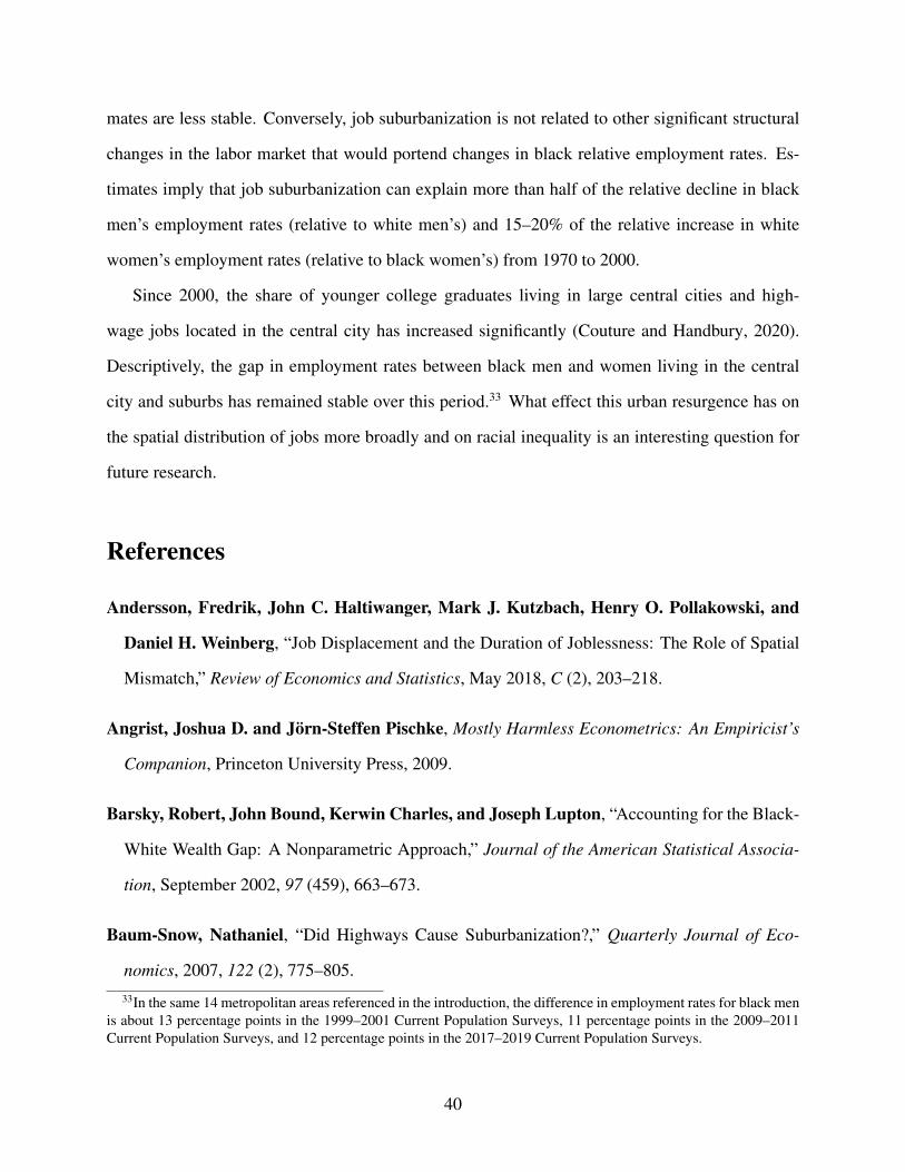
mates are less stable. Conversely, job suburbanization is not related to other significant structural

changes in the labor market that would portend changes in black relative employment rates. Es-

timates imply that job suburbanization can explain more than half of the relative decline in black

men’s employment rates (relative to white men’s) and 15–20% of the relative increase in white

women’s employment rates (relative to black women’s) from 1970 to 2000.

Since 2000, the share of younger college graduates living in large central cities and high-

wage jobs located in the central city has increased significantly (Couture and Handbury, 2020).

Descriptively, the gap in employment rates between black men and women living in the central

city and suburbs has remained stable over this period.33 What effect this urban resurgence has on

the spatial distribution of jobs more broadly and on racial inequality is an interesting question for

future research.

References

Andersson, Fredrik, John C. Haltiwanger, Mark J. Kutzbach, Henry O. Pollakowski, and

Daniel H. Weinberg, “Job Displacement and the Duration of Joblessness: The Role of Spatial

Mismatch,” Review of Economics and Statistics, May 2018, C (2), 203–218.

Angrist, Joshua D. and Jorn-Steffen Pischke, Mostly Harmless Econometrics: An Empiricist’s

Companion, Princeton University Press, 2009.

Barsky, Robert, John Bound, Kerwin Charles, and Joseph Lupton, “Accounting for the Black-

White Wealth Gap: A Nonparametric Approach,” Journal of the American Statistical Associa-

tion, September 2002, 97 (459), 663–673.

Baum-Snow, Nathaniel, “Did Highways Cause Suburbanization?,” Quarterly Journal of Eco-

nomics, 2007, 122 (2), 775–805.33In the same 14 metropolitan areas referenced in the introduction, the difference in employment rates for black men

is about 13 percentage points in the 1999–2001 Current Population Surveys, 11 percentage points in the 2009–2011Current Population Surveys, and 12 percentage points in the 2017–2019 Current Population Surveys.

40

, “Urban Transport Expansions and Changes in the Spatial Structure of US Cities: Implications

for Productivity and Welfare,” Review of Economics and Statistics, forthcoming. Unpublished

manuscript.

Bayer, Patrick, Hanming Fang, and Robert McMillan, “Separate when equal? Racial inequality

and residential segregation,” Journal of Urban Economics, July 2014, 82, 32–48.

Blau, Francine D. and John W. Graham, “Black-White Differences in Wealth and Asset Com-

position,” Quarterly Journal of Economics, 1990, 105 (2), 321–339.

Boustan, Leah, “Was Postwar Suburbanization ”White Flight”? Evidence from the Black Migra-

tion,” Quarterly Journal, February 2010, 125 (1), 417–443.

Carrington, William J., Kristin McCue, and Brooks Pierce, “Using Establishment Size to Mea-

sure the Impact of Title VII and Affirmative Action,” Journal of Human Resources, Summer

2000, 35 (3), 503–523.

Cattaneo, Matias, Richard Crump, Max Farrell, and Yingjie Feng, “On Binscatter,” 2019.

Unpublished manuscript.

Coulson, Edward, Derek Laing, and Paul Wang, “Spatial Mismatch in Search Equilibrium,”

Journal of Labor Economics, October 2001, 19 (4), 949–972.

Couture, Victor and Jessie Handbury, “Urban Revival in America,” Journal of Urban Eco-

nomics, September 2020, 119. Unpublished manuscript.

Cutler, David M., Edward L. Glaeser, and Jacob L. Vigdor, “The Rise and Decline of the

American Ghetto,” Journal of Political Economy, June 1999, 107 (3), 455–506.

Duranton, Giles, Peter M. Morrow, and Matthew A. Turner, “Roads and Trade: Evidence from

the US,” Review of Economic Studies, April 2014, 81 (2), 681–724.

Duraton, Giles and Matt Turner, “Urban Growth and Transformation,” Review of Economic

Studies, October 2012, 79 (4), 1407–1440.

41

Ellwood, David T., “The spatial mismatch hypothesis: Are there teenage jobs missing in the

ghetto?,” in Richard B. Freeman and Harry J. Holzer, eds., The black youth employment crisis,

Chicago: University of Chicago Press, 1986.

Evans, William N., Craig Garthwaite, and Timothy J. Moore, “The White/Black Educational

Gap, Stalled Progress, and the Long-Term Consequences of the Emergence of Crack Cocaine

Markets,” Review of Economics and Statistics, December 2016, 98 (5), 832–847.

Fairlie, Robert W. and William A. Sundstrom, “The Emergence, Persistence, and Recent

Widening of the Racial Unemployment Gap,” Industrial and Labor Relations Review, January

1999, 52 (2), 252–270.

Fernandez, Roberto M., “Race, spatial mismatch, and job accessibility: Evidence from a plant

relocation,” Social Science Research, September 2008, 37 (3), 953–975.

Glaeser, Ed and Matthew Kahn, “Decentralized Employment and the Transformation of the

American City,” Brookings-Wharton Papers on Urban Affairs, 2001, 2.

Guryan, Jonathan, “Desegregation and Black Dropout Rates,” American Economic Review,

September 2004, 94 (4), 919–943.

Hellerstein, Judith K., David Neumark, and Melissa McInerney, “Spatial mismatch or racial

mismatch?,” Journal of Urban Economics, 2008, 64, 464–479.

Holian, Matthew J. and Matthew E. Kahn, The Impact of Center City Economic and Cultural

Vibrancy on Greenhouse Gas Emissions from Transportation, San Jose, CA: MTI Publications,

2012.

Holzer, Harry J. and Keith R. Ihlanfeldt, “Spatial factors and the employment of blacks at the

firm level,” New England Economic Review, May/June 1996, 65.

42

Ihlanfeldt, Keith R. and David L. Sjoquist, “The Spatial Mismatch Hypothesis: A Review of

Recent Studies and Their Implications for Welfare Reform,” Housing Policy Debate, 1998, 9

(4), 849–892.

Johnson, Rucker, “Landing a Job in Urban Space: the Extent and Effects of Spatial Mismatch,”

Regional Science and Urban Economics, 2006, 36, 331–372.

Kain, John F., “Housing Segregation, Negro Employment and Metropolitan Decentralization,”

Quarterly Journal of Economics, 1968, 82 (3), 175–197.

Michaels, Guy, “The Effect of Trade on the Demand for Skill: Evidence from the Interstate

Highway System,” Review of Economics and Statistics, 2008, 90 (4), 683–701.

Mouw, Ted, “Job Relocation and the Racial Gap in Unemployment in Detroit and Chicago 1980-

1990: a Fixed-Effects Estimate of the Spatial Mismatch Hypothesis,” American Sociological

Review, 2000, 65, 730–753.

Phillips, David C., “Do Low-Wage Employers Discriminate Against Applicants with Long Com-

mutes?: Evidence from a Correspondence Experiment,” Journal of Human Resources, Summer

2020, 55 (3), 864–901.

Raphael, Steven, “The Spatial Mismatch Hypothesis and Black Youth Joblessness: Evidence from

the San Francisco Bay Area,” Journal of Urban Economics, 1998, 43, 79–111.

Raphel, Steven, Michael A. Stoll, and Harry J. Holzer, “Are Suburban Firms More Likely to

Discriminate against African-Americans?,” Journal of Urban Economics, November 2000, 48

(3), 485–508.

Ritter, Joseph A. and Lowell J. Taylor, “Racial Disparity in Unemployment,” Review of Eco-

nomics and Statistics, February 2011, 93 (1), 30–42.

Robinson, Corre L., Tiffany Taylor, Donald Tomaskovic-Devey, Catherine Zimmer, and

Matthew W. Irvin, “Studying Race or Ethnic and Sex Segregation at the Establishment Level:

43

Methodological Issues and Substantive Opportunities Using EEO-1 Reports,” Work and Occu-

pations, February 2005, 32 (1), 5–38.

Rose, Mark H. and Raymond A. Mohl, Interstate: Highway Politics and Policy since 1939,

Knoxville: The University of Tennessee Press, 2012.

Rothstein, Richard, The Color of Law: A Forgotten History of How Our Government Segregated

America, first ed., London: Liveright Publishing Corporation, 2017.

Rothwell, Jonathan T., “Racial Enclaves and Density Zoning: The Institutionalized Segregation

of Racial Minorities in the United States,” American Law and Economics Review, Spring 2011,

13 (1), 290–358.

and Douglas S. Massey, “The Effect of Density Zoning on Racial Segregation in U.S. Urban

Areas,” Urban Affairs Review, 2009, 44 (6), 779–806.

Ruggles, Steven, J. Trent Alexander, Katie Genadek, Ronald Goeken, Matthew B. Schroeder,

and Matthew Sobek, “Integrated Public Use Microdata Series: Version 5.0 [Machine-readable

database],” Minneapolis: University of Minnesota 2010.

Stoll, Michael A., “Job Sprawl, Spatial Mismatch, and Black Employment Disadvantage,” Journal

of Policy Analysis and Management, 2006, 25 (4), 827–854.

Weinberg, Bruce A., Patricia B. Reagan, and Jeffrey J. Yankow, “Do Neighborhoods Affect

Hours Worked? Evidence from Longitudinal Data,” Journal of Labor Economics, October 2004,

22 (4), 891–924.

Western, Bruce and Becky Pettit, “Incaraceration and Racial Inequality in Men’s Employment,”

Industrial and Labor Relations Review, October 2000, 54 (1), 3–16.

Wilson, William Julius, The Truly Disadvantaged: The Inner City, the Underclass and Public

Policy, Chicago, IL: University of Chicago Press, 1987.

44

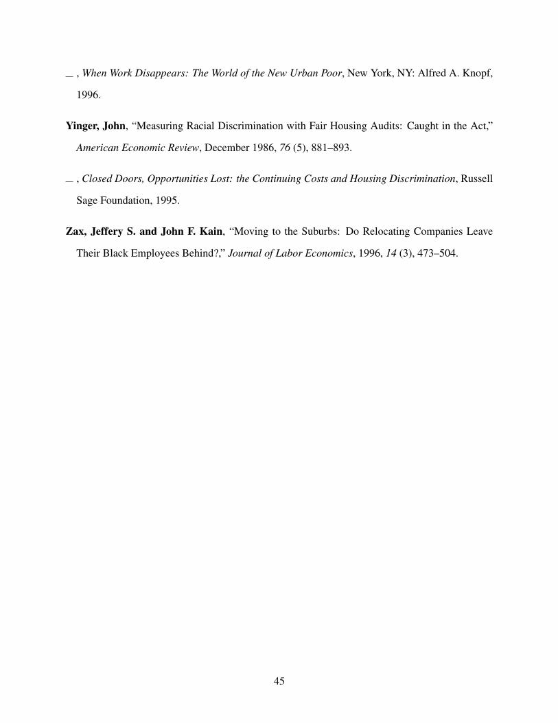
, When Work Disappears: The World of the New Urban Poor, New York, NY: Alfred A. Knopf,

1996.

Yinger, John, “Measuring Racial Discrimination with Fair Housing Audits: Caught in the Act,”

American Economic Review, December 1986, 76 (5), 881–893.

, Closed Doors, Opportunities Lost: the Continuing Costs and Housing Discrimination, Russell

Sage Foundation, 1995.

Zax, Jeffery S. and John F. Kain, “Moving to the Suburbs: Do Relocating Companies Leave

Their Black Employees Behind?,” Journal of Labor Economics, 1996, 14 (3), 473–504.

45

A Appendix (For Online Publication)

A.1 Establishment Relocations and Occupational Composition

While the sharp pattern in Figure 2 suggests that relocation causes a decline in the black shareof employees, it is possible that change in the racial composition of employees are driven bycoincident changes within the establishment rather than the relocation per se. In particular, thetypes of work performed at an establishment may change following relocation in a way that wouldaffect the racial composition of employees. In this section I apply an event study research designanalogous to (2) where the outcome is an establishment’s predicted black share of employees givenits industry, occupation mix, and Census division. To predict black share, I take each establishmentby occupation pair and calculate the black share of employees in that industry, occupation, andCensus division in a given year, excluding the establishment itself. I plot the θ coefficients inFigure A1.

A.2 Highways and Residential Suburbanization

To determine the relationship between highways and residential suburbanization and segregation,I estimate MSA-level regressions rather than group-level regressions. I do this because I cannotobserve whether individuals live in the central city in the 1970 Census. Instead, I use populationdata from the County and City Data Books (CCDB), which report decennial Census data aggre-gated to counties and cities of at least 25000 inhabitants. For the household suburbanization andsegregation analysis, I estimate specifications of the following form:

∆Ym = δ1rays1970m + δ2radius

ccm + εm (A.8)

where Y denotes either log πccres, where πccres is the fraction of an MSA’s population living in thecentral city, or the dissimilarity index. I estimate this model for the whole population and separatelyby race when the outcome is household suburbanization.

I present estimates in Table A6. Again, actual interstate highway rays constructed is the ex-planatory variable in odd columns, while highway rays are instrumented using planned rays in evencolumns. Highway rays predict the suburbanization of white households, but not black households.This disparity is consistent with a central premise of the spatial mismatch hypothesis: black house-holds faced significant additional barriers to suburban residence over this period. Each ray predictsa 4.7%, 8.2%, and 10.2% decline in the central city share of the white population by 1980, 1990,and 2000. By contrast, highways predict only a negligible decline in the black population. Theeffects are more negative when I instrument for highway construction, though the effect on the

46

black central city population remains statistically insignificant. This is consistent with the premisethat black households faced significant additional barriers to suburban residence. The IV coeffi-cients are consistent with Baum-Snow (forthcoming) who finds that that each new radial highwaydecentralized 14-16% of central city working residents from 1960 to 2000 in a larger set of MSAs.Highway rays increase subsequent segregation, with each ray predicting an increase of 0.010,0.045, and 0.053 point increase in a city’s dissimilarity index.

A.3 Job Suburbanization and Sector Composition

The spatial distribution of jobs shifted towards the suburban ring while the structure of the USlabor market was changing in other important ways. From World War II to the late 1970s, therelative supply of college-educated workers rose substantially (Autor et al., 2008). The manufac-turing share of employment has declined consistently since World War II. Since 1980, there hasbeen a pronounced increase in wage inequality and job polarization–employment and wage gainsin low and high skilled occupations relative to middle skill occupations–both of which have beenattributed by many researchers to technological change (Acemoglu and Autor, 2011). Job subur-banization may have occurred as part of a joint process with these and other fundamental changesin the labor market, which would complicate teasing out the causal implications of suburbaniza-tion. In this section, I explore whether job suburbanization is associated with changes in the typesof work performed in the labor market.

To evaluate the importance of sector shifts associated with job suburbanization, I test whetherMSAs with greater exposure to the interstate highway system or that experience greater job sub-urbanization also experience relative growth in the sectors that disproportionately employed whiteor black workers in 1970. Specifically, for each cell mg I measure the share of workers in 1970that are employed in major sector s, ωsmg, where sectors are defined by major industry.34 Let πsmtdenote the share of employment in market m at time t that is in sector s. For each cell I constructa weighted average of sector growth,

growthtmg =∑s

ωsmg (log πsmt′ − log πsm70) . (A.9)

In words, growthtmg captures the extent to which sectors in which cell mg disproportionatelyworked in 1970 grow relative to other sectors. I first estimate equation (7) replacing the outcome

34The major industry categories I use are: (1) agriculture, forestry, and fisheries; (2) mining; (3) construction; (4)nondurable goods manufacturing; (5) durable goods manufacturing; (6) transportation, communications, and otherpublic utilities; (7) wholesale trade; (8) retail trade; (9) finance, insurance, and real estate; (10) business and repairservices; (11) personal, entertainment, and recreation services; (12) profession services, health; (13) professionalservices, education; (14) professional services, other; and (15) public administration.

47

with growthtmg to evaluate whether interstate highways cause changes in sector composition thatfavor sectors where black or white workers are concentrated at baseline. I also repeat this exerciseclassifying sectors by major occupation rather than industry.35

Table A7 presents the results. As above, columns (1), (4), and (7) are OLS models, in remainingspecifications I instrument for actual highway rays using planned highway rays, and columns (3),(6), and (9) include MSA-by-education fixed effects. In the top panel, growthtmg is industry-based;in the bottom panel, growthtmg is occupation-based.

For the industry-based measure, all β and βB coefficients are statistically insignificant andsmall in magnitude. Hence, highways do not predict changes in relative growth or declines inindustries where black workers were concentrated in 1970.

For the occupation-based measure, β is statistically insignificant in all specifications. βB isstatistically insignificant for the 1970-1980 period, when the relationship between highways andblack relative employment rates emerges in Table 5. By contrast the βB is statistically significantin columns (4) and (5) for the 1970-1990 period and columns (7) and (8) for the 1970-2000 period,ranging from -0.013 to -0.017. This indicates that highways predict relative declines in occupationswhere black workers were concentrated in 1970. Yet this relationship merges after the relationshipbetween highways and black relative employment rates emerges. Moreover, this coefficient be-comes statistically insignificant with the inclusion of MSA-by-education fixed effects in columns(6) and (9). Hence, the relationship between highway rays and occupation-based sector growthfor black workers appears to be driven by educational differences. On the other hand, as shown inTable 5, the relationship between highway rays and black relative employment rates holds within

education groups. I conclude that the causal effect of interstate highways on racial differences inemployment rates is not driven by changes in sector composition.

Next, I repeat the exercise but look at job suburbanization more broadly rather than subur-banization induced by interstate highways. I estimate equation (4) replacing the outcome withgrowthtmg to evaluate whether job suburbanization is associated with changes in sector composi-tion that favor sectors where black or white workers are concentrated at baseline.

Table A9 presents the results, replicating Table 4 in structure. In columns (1)-(3) the periodis 1970 to 1980, in columns (4)-(6) the period is 1970-1990, and in columns (7)-(9) the periodis 1970 to 2000. All columns include group fixed effects. Columns excluding (1), (4), and (7)include controls for a quadratic in baseline employment rates or log average earnings interactedwith race. Columns (3), (6), and (9) include MSA-by-education fixed effects. In the top panel,

35The major occupation categories I use are: (1) executive, administrative, and managerial occupations; (2) profes-sional specialty occupations; (3) technicians and related support occupations; (4) sales occupations; (5) administrativesupport occupations, including clerical; (6) service occupations; (7) farming, forestry, and fishing occupations; (8)precision production, craft, and repair occupations (9) operators, fabricators, and laborers; and (10) military occupa-tions.

48

growthtmg is industry-based; in the bottom panel, growthtmg is occupation-based. For the industry-based measure, βB is negative and marginally significant at the 10% level for the 1970-1980 periodin each specification. This indicates that job suburbanization is associated with relative growth

in industries where black workers were concentrated in 1970, when in fact suburbanization isassociated with relative declines in black employment rates. For the 1970-1990 and 1970-2000periods, βB coefficients are statistically insignificant.

For the occupation-based measure, βB is statistically significant and positive in columns (4)and (5) for the 1970-1990 period. This coefficient becomes statistically insignificant in column(6) with the inclusion of MSA-by-education fixed effects. For the remaining specifications βB

is statistically insignificant. I conclude that job suburbanization is generally not associated withchanges in sector composition that would portend declines in black employment rates.

A.4 Endogenous Migration

Due to data limitations, I conduct the main analysis using a synthetic panel rather than a true panelof individuals. For the same reason that residential sorting is a concern for any cross-sectionalanalysis, the endogenous migration of households to and from MSAs may introduce a composi-tional bias in the synthetic panel analysis. The productivity of migrants to and from an MSA mayvary systematically with job suburbanization, so that the correlation between job suburbanizationand employment growth may in part reflect the changing composition of cells rather than within-person changes. For example, productive black households may move out of an MSA followingwidespread suburbanization, leaving less productive black households behind. While this typeof endogenous migration would suggest that the spatial distribution of work is relevant for labormarket outcomes, it complicates the interpretation of the coefficient estimates.

In assessing the role of migration, I focus on the 1970-1980 period, where job suburbanizationappears to have its largest effect.36 I utilize the fact that the 1980 Census identifies an individual’splace of residence and employment status in 1975 for half the sample. Hence, I observe a truepanel of a large subsample of individuals over this 5-year period. I estimate models analogous to(4), except over a 5-year period, and compare the results when using a synthetic panel to resultsusing a true panel. I construct the synthetic panel by assigning individuals to MSAs separately bywhere they live in 1975 and where they live in 1980. To form the true panel, I assign individualsto MSAs based only on where they live in 1975.

Unfortunately, I cannot observe the spatial distribution of work in 1975. Instead, I halve thesame measure of job suburbanization from over the 10-year period. Note that, even under randommigration, the coefficients in the true panel analysis may be attenuated for the same reason that

36While data limitations prevent me from studying migration at the same level of detail over the full period, I dofind that changes in cell size from 1970 to 2000 are unrelated to job suburbanization.

49

attrition attenuates coefficient estimates. Households that move are mechanically less ‘exposed’to job suburbanization in their assigned MSA than households that do not move. Under randommigration, given that about 15% of individuals change MSAs over this period, and assuming coef-ficients of zero for moving households, this attrition would predict that the coefficients in the truepanel analysis is about 85% as large as the coefficients in the synthetic panel analysis.

I present estimates from the 5-year analysis in Table A8. In columns (1) and (2) the outcomeis ∆ log (Fraction Employed). In column (1) the analysis is conducted using a true panel; column(2) is estimated using a synthetic panel. In general, the coefficients do not differ substantially. Aswould roughly be predicted by random migration, the coefficient on ∆ log(πccm) × black is about15% smaller in magnitude under the true panel, and statistically significant using either the true orsynthetic panel.

In addition, I test directly for selective migration by examining whether job suburbanizationpredicts migration flows and the composition of migrants. For migration flows I look at the fractionof a cell that emigrates out of the original MSA. Column (3) presents coefficient estimates fromthis exercise. To examine the composition of emigrants, I look at how the 1975 employment rateof a cell would change if the eventual migrants were excluded (I label this as ∆M(emp)). Column(4) presents coefficient estimates from this exercise. While job suburbanization predicts a small,marginally significant decrease in emigration for white cells, it is uncorrelated with changes in thecomposition of cells due to emigration.

50

FIGURE A1: Establishment Relocations and Occupation Composition

Notes: These figures plot event study coefficients and 95% confidence intervals (dotted) estimated using model (2)where the outcome is an establishment’s predicted black share of employees given industry, occupation mix, andCensus division. The models are estimated using all establishments that relocate from the central city to the suburbsand whose distance from the central business district increases by at least 5 miles and establishments that remain inthe central city. The coefficient for the year prior to the event (θ−1) is normalized to zero. Estimated models includeCensus division by year fixed effects and log establishment size as controls. Standard errors are clustered at theestablishment level.

51

FIG

UR

EI

The

Pro

ject

edSy

stem

ofIn

ters

tate

Hig

hway

sin

1947

780 QUARTERLY JOURNAL OF ECONOMICS

at MIT Libraries on February 2, 2012

http://qje.oxfordjournals.org/D

ownloaded from

FIG

UR

EA

2:19

47In

ters

tate

Hig

hway

Plan

Not

es:T

his

figur

eis

take

nfr

omB

aum

-Sno

w(2

007)

.

52

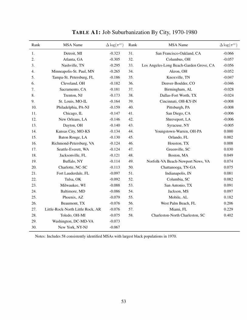
TABLE A1: Job Suburbanization By City, 1970-1980

Rank MSA Name ∆ log(πcc) Rank MSA Name ∆ log(πcc)

1. Detroit, MI -0.323 31. San Francisco-Oakland, CA -0.0662. Atlanta, GA -0.305 32. Columbus, OH -0.0573. Nashville, TN -0.295 33. Los Angeles-Long Beach-Garden Grove, CA -0.0564. Minneapolis-St. Paul, MN -0.265 34. Akron, OH -0.0525. Tampa-St. Petersburg, FL -0.186 35. Knoxville, TN -0.0476. Cleveland, OH -0.182 36. Denver-Boulder, CO -0.0467. Sacramento, CA -0.181 37. Birmingham, AL -0.0288. Trenton, NJ -0.173 38. Dallas-Fort Worth, TX -0.0249. St. Louis, MO-IL -0.164 39. Cincinnati, OH-KY-IN -0.00810. Philadelphia, PA-NJ -0.159 40. Pittsburgh, PA -0.00811. Chicago, IL -0.147 41. San Diego, CA -0.00612. New Orleans, LA -0.146 42. Shreveport, LA -0.00613. Dayton, OH -0.140 43. Syracuse, NY -0.00514. Kansas City, MO-KS -0.134 44. Youngstown-Warren, OH-PA 0.00015. Baton Rouge, LA -0.130 45. Orlando, FL 0.00216. Richmond-Petersburg, VA -0.124 46. Houston, TX 0.00817. Seattle-Everett, WA -0.124 47. Greenville, SC 0.03018. Jacksonville, FL -0.121 48. Boston, MA 0.04919. Buffalo, NY -0.114 49. Norfolk-VA Beach-Newport News, VA 0.07420. Charlotte, NC-SC -0.113 50. Chattanooga, TN-GA 0.07521. Fort Lauderdale, FL -0.097 51. Indianapolis, IN 0.08122. Tulsa, OK -0.092 52. Columbia, SC 0.08223. Milwaukee, WI -0.088 53. San Antonio, TX 0.09124. Baltimore, MD -0.086 54. Jackson, MS 0.09725. Phoenix, AZ -0.079 55. Mobile, AL 0.18226. Beaumont, TX -0.076 56. West Palm Beach, FL 0.20627. Little-Rock-North Little Rock, AR -0.076 57. Miami, FL 0.22928. Toledo, OH-MI -0.075 58. Charleston-North Charleston, SC 0.40229. Washington, DC-MD-VA -0.07330. New York, NY-NJ -0.067

Notes: Includes 58 consistently identified MSAs with largest black populations in 1970.

53

TABLE A2: Job Suburbanization By City, 1970-2000

Rank MSA Name ∆ log(πcc) Rank MSA Name ∆ log(πcc)

1. Detroit, MI -0.804 31. San Francisco-Oakland, CA -0.2702. Atlanta, GA -0.742 32. Kansas City, MO-KS -0.2173. Richmond-Petersburg, VA -0.709 33. Pittsburgh, PA -0.1974. St. Louis, MO-IL -0.645 34. Orlando, FL -0.1905. Minneapolis-St. Paul, MN -0.567 35. Beaumont, TX -0.1696. Dayton, OH -0.560 36. Charleston-North Charleston, SC -0.1677. Cleveland, OH -0.502 37. Houston, TX -0.1678. Denver-Boulder, CO -0.493 38. Mobile, AL -0.1659. Baltimore, MD -0.487 39. Boston, MA -0.16510. Philadelphia, PA-NJ -0.439 40. Knoxville, TN -0.14811. Sacramento, CA -0.439 41. Los Angeles-Long Beach-Garden Grove, CA -0.14112. Trenton, NJ -0.432 42. Jackson, MS -0.13013. Cincinnati, OH-KY-IN -0.432 43. Little Rock-North Little Rock, AR -0.07714. Fort Lauderdale, FL -0.428 44. Nashville, TN -0.07715. Washington, DC-MD-VA -0.419 45. Columbus, OH -0.07216. Chicago, IL -0.407 46. San Diego, CA -0.06317. Seattle-Everett, WA -0.396 47. Columbia, SC -0.05418. Milwaukee, WI -0.393 48. Tulsa, OK -0.05019. Buffalo, NY -0.378 49. Indianapolis, IN -0.02820. Dallas-Fort Worth, TX -0.358 50. Baton Rouge, LA -0.02621. Birmingham, AL -0.349 51. Jacksonville, FL -0.01222. Youngstown-Warren, OH-PA -0.349 52. Shreveport, LA -0.00923. New Orleans, LA -0.338 53. Charlotte, NC-SC 0.00624. Syracuse, NY -0.329 54. New York, NY-NJ 0.01825. Tampa, FL -0.323 55. San Antonio, TX 0.03626. Miami, FL -0.322 56. Norfolk-VA Beach-Newport News, VA 0.10027. Greenville, SC -0.314 57. Chattanooga, TN-GA 0.10128. Toledo, OH-MI -0.311 58. West Palm Beach, FL 0.10629. Akron, OH -0.28830. Phoenix, AZ -0.285

Notes: Includes 58 consistently identified MSAs with largest black populations in 1970.

54

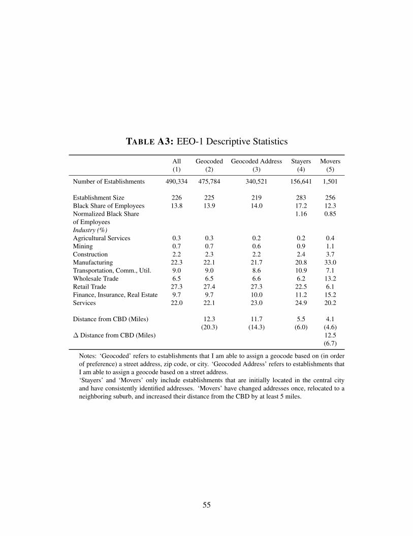
TABLE A3: EEO-1 Descriptive Statistics

All Geocoded Geocoded Address Stayers Movers(1) (2) (3) (4) (5)

Number of Establishments 490,334 475,784 340,521 156,641 1,501

Establishment Size 226 225 219 283 256Black Share of Employees 13.8 13.9 14.0 17.2 12.3Normalized Black Share 1.16 0.85of EmployeesIndustry (%)Agricultural Services 0.3 0.3 0.2 0.2 0.4Mining 0.7 0.7 0.6 0.9 1.1Construction 2.2 2.3 2.2 2.4 3.7Manufacturing 22.3 22.1 21.7 20.8 33.0Transportation, Comm., Util. 9.0 9.0 8.6 10.9 7.1Wholesale Trade 6.5 6.5 6.6 6.2 13.2Retail Trade 27.3 27.4 27.3 22.5 6.1Finance, Insurance, Real Estate 9.7 9.7 10.0 11.2 15.2Services 22.0 22.1 23.0 24.9 20.2

Distance from CBD (Miles) 12.3 11.7 5.5 4.1(20.3) (14.3) (6.0) (4.6)

∆ Distance from CBD (Miles) 12.5(6.7)

Notes: ‘Geocoded’ refers to establishments that I am able to assign a geocode based on (in orderof preference) a street address, zip code, or city. ‘Geocoded Address’ refers to establishments thatI am able to assign a geocode based on a street address.‘Stayers’ and ‘Movers’ only include establishments that are initially located in the central cityand have consistently identified addresses. ‘Movers’ have changed addresses once, relocated to aneighboring suburb, and increased their distance from the CBD by at least 5 miles.

55

TABLE A4: Heterogeneous Effects of Job Suburbanization

1970-2000HS Dropout HS Grad College Grad Men Women

Y: ∆ log (Emp. Rate) (1) (2) (3) (4) (5)

∆ log(πcc) 0.017 -0.029 -0.039 -0.008 -0.036(0.070) (0.039) (0.035) (0.029) (0.050)

∆ log(πcc) × black 0.216** 0.098** 0.083* 0.118** 0.169**(0.062) (0.035) (0.040) (0.036) (0.047)

Y: ∆ log (Avg. Earnings)

∆ log(πcc) 0.077 0.023 0.016 0.065 0.004(0.101) (0.071) (0.066) (0.057) (0.088)

∆ log(πcc) × black 0.144 0.107˜ 0.125 -0.008 0.233*(0.093) (0.062) (0.096) (0.077) (0.090)

Group FEs Yes Yes Yes Yes YesBaseline Controls Yes Yes Yes Yes YesN Cells 206 218 139 275 287N MSAs 58 58 58 58 58

Notes: Table displays estimates of equation (4) covering 1970-2000. Column (1) restricts to cells withless than high school degree, column (2) restricts to high school graduates, column (3) restricts to collegegraduates, column (4) restricts to men, and column (5) restricts to women. All models include groupfixed effects (fixed effects for all combinations of cohort, education, sex, and race) and a quadratic in logbaseline employment (Panel A) or log average earnings (Panel B) interacted with race. In Panel A, theoutcome is changes in log employment rates; in Panel B, the outcome is changes in log earnings. Allmodels are estimated at the cell level.˜ Denotes statistical significance at the p < 0.10 level. * Denotes statistical significance at p < 0.05

level. ** Denotes statistical significance at p < 0.01 level.Standard errors in parentheses, clustered at the MSA level. Regression weighted by cell size.

56

TABLE A5: Highways and Baseline Cell and MSACharacteristics

Panel A: Highways and Employment (1965-1970)Outcome: ∆PRE log (Employment Rate) (1) (2)

Rays -0.000(.003)

Rays × black -0.004(.003)

N Cells 2016N MSAs 56

Panel B: Highways and 1970 Characteristics δ δB

Outcome: Rays

Log Fraction Active (Group) -4.310** .879(1.536) (1.194)

Log Earnings (Group) 3.377* -0.905(1.291) (0.718)

Fraction of Work in Central City (MSA), -0.013 0.133Standardized (0.273) (0.154)Fraction Black (MSA), 0.064 0.157Standardized (0.262) (0.166)Dissimilarity Index (MSA), 0.383 0.206˜Standardized (0.294) (0.114)Violent Crime Rate (MSA), 0.196 -0.128Standardized (0.321) (0.129)Property Crime Rate (MSA), -0.441 -0.076Standardized (0.270) (0.130)

N Cells 1516N MSAs 54

Notes: Panel A displays estimates of equation (5) with ∆ log(πcc) re-placed by highway rays in 1970. In Panel A, the outcome is cell-levelchanges in employment rates from 1965 to 1970. Panel B displays esti-mates of equation (6) ∆ log(πcc) replaced by highway rays in 1970. Inthis panel, the outcome is highway rays in 1970. Column (1) displaythe estimated δ coefficients from equation (6), the ‘main effects’; col-umn (2) display the estimated δB coefficients, the black cell interactions.All models include group fixed effects (fixed effects for all combinationsof cohort, education, sex, and race) and a control for central city radius.Dissimilarity segregation indices are taken from Cutler et al. (1999). TwoMSAs are not included in the highway data (Baum-Snow, 2007): Jack-son, MS and West Palm Beach, FL. Dissimilarity segregation indices aretaken from (Cutler et al., 1999). Standard errors in parentheses, clusteredat the MSA level. Regression weighted by cell size. ˜ Denotes statisticalsignificance at the p < 0.10 level. * Denotes statistical significance atp < 0.05 level. ** Denotes statistical significance at p < 0.01 level.

57

TABLE A6: Highways, Residential Suburbanization, and Segregation,1970-2000

1970-1980 1970-1990 1970-2000OLS IV OLS IV OLS IV

Outcome: ∆ log(πccres), White (1) (2) (3) (4) (5) (6)

Rays -0.047** -0.077** -0.082** -0.137** -0.102* -0.180**(0.014) (0.023) (0.028) (0.041) (0.039) (0.058)

CC Radius Control Yes Yes Yes Yes Yes YesN MSAs 56 56 56 56 56 56

Outcome: ∆ log(πccres), Black

Rays 0.006 -0.006 0.003 -0.022 -0.005 -0.050(0.011) (0.018) (0.021) (0.033) (0.036) (0.054)

CC Radius Control Yes Yes Yes Yes Yes YesN MSAs 56 56 56 56 56 56

Outcome: ∆ log(Dissimilarity)

Rays 0.010 0.026 0.045** 0.048* 0.053** 0.056*(0.013) (0.014) (0.011) (0.021) (0.016) (0.026)

CC Radius Control Yes Yes Yes Yes Yes YesN MSAs 56 56 56 56 56 56

Notes: Table displays estimates of equation (A.8). All models include controls for central city radius.Even columns instrument for actual highway rays in 1970 with planned highways. Dissimilarity seg-regation indices are taken from Cutler et al. (1999). Two MSAs are not included in the highway data(Baum-Snow, 2007): Jackson, MS and West Palm Beach, FL. Standard errors in parentheses, clusteredat the MSA level. Regression weighted by MSA population. Data from County and City Data Books. ˜Denotes statistical significance at the p < 0.10 level. * Denotes statistical significance at p < 0.05 level.** Denotes statistical significance at p < 0.01 level.

58

TABLE A7: Highways and Sector Composition, 1970-2000

1970-1980 1970-1990 1970-2000

Outcome: Industry-Based Sector Growth OLS IV IV OLS IV IV OLS IV IV(1) (2) (3) (4) (5) (6) (7) (8) (9)

Rays1970 -0.000 0.001 -0.002 -0.003 0.001 -0.005(0.001) (0.001) (0.002) (0.003) (0.003) (0.004)

Rays1970 0.007 0.006 0.008 0.002 -0.002 0.003 -0.002 -0.007 0.001× black (0.004) (0.005) (0.006) (0.005) (0.006) (0.008) (0.005) (0.007) (0.008)

Outcome: Occupation-Based Sector Growth

Rays1970 -0.002 -0.002 0.001 -0.001 0.002 -0.000(0.002) (0.003) (0.003) (0.004) (0.004) (0.005)

Rays1970 -0.003 -0.003 0.002 -0.013** -0.014* -0.004 -0.015** -0.017* -0.006× black (0.004) (0.006) (0.004) (0.004) (0.011) (0.005) (0.004) (0.007) (0.007)

Group FEs Yes Yes Yes Yes Yes Yes Yes Yes YesMSA × Education FEs No No Yes No No Yes No No YesBaseline Controls Yes Yes Yes Yes Yes Yes Yes Yes YesCC Radius Control Yes Yes Yes Yes Yes Yes Yes Yes YesN Cells 1559 1559 1559 1066 1066 1066 545 545 545N MSAs 56 56 56 56 56 56 56 56 56

Notes: Table displays estimates of equation (7) where the outcome is growthtmg , a weighted average of sector growthwith cell-specific weights. This measure captures the extent to which sectors in which cell mg disproportionatelyworked in 1970 grow relative to other sectors. In the top panel, sectors are industry-based; in the bottom panel, sectorsare occupation-based. See section A.3 for further details. All models include controls for central city radius. Two MSAsare not included in the highway data (Baum-Snow, 2007): Jackson, MS and West Palm Beach, FL. Standard errors inparentheses, clustered at the MSA level. Regression weighted by MSA population. ˜ Denotes statistical significance atthe p < 0.10 level. * Denotes statistical significance at p < 0.05 level. ** Denotes statistical significance at p < 0.01

level.

59

TABLE A8: Job Suburbanization, Employment, and Migration,1975-1980

∆ log (Emp. Rate) Fraction ∆ log (Emp. Rate)True Synthetic Emigrate Baseline(1) (2) (3) (4)

∆ log(πcc) 0.078 0.017 0.112* 0.012(0.065) (0.086) (0.056) (0.010)

∆ log(πcc) × black 0.291* 0.368* -0.060 0.003(0.116) (0.158) (0.059) (0.009)

Group FEs Yes Yes Yes YesBaseline Controls Yes Yes Yes YesN Cells 1682 1682 1682 1682N MSAs 58 58 58 58

Notes: Table displays estimates of equation (4) covering 1975-1980. In columns (1)and (2), the outcome is changes in log employment rates, measured using a ‘true’ panelin column (1) and using a ‘synthetic’ panel in column (2). In column (3) the outcomeis the fraction emigrating from their initial MSA. In column (4) the outcome is thedifference between the 1975 employment rate excluding eventual migrants and the 1975employment including eventual migrants. See section A.4 for further details on howthese outcomes are constructed.Notes: ˜ Denotes statistical significance at the p < 0.10 level. * Denotes statisticalsignificance at p < 0.05 level. ** Denotes statistical significance at p < 0.01 level.Standard errors in parentheses, clustered at the MSA level. Regression weighted by cellsize.

60

TAB

LE

A9:

Job

Subu

rban

izat

ion

and

Sect

orC

ompo

sitio

n

1970

-198

019

70-1

990

1970

-200

0

Out

com

e:In

dust

ry-B

ased

Sect

orG

row

th(1

)(2

)(3

)(4

)(5

)(6

)(7

)(8

)(9

)

∆lo

g(π

cc)

0.00

00.

003

0.00

40.

007

0.00

50.

007

(0.0

12)

(0.0

12)

(0.0

11)

(0.0

10)

(0.0

17)

(0.0

16)

∆lo

g(π

cc)×

blac

k-0

.095

˜-0

.081

˜-0

.089

˜0.

052

0.03

90.

026

0.05

50.

032

0.02

7(0

.049

)(0

.044

)(0

.052

)(0

.052

)(0

.042

)(0

.059

)(0

.033

)(0

.030

)(0

.051

)

Out

com

e:In

dust

ry-B

ased

Sect

orG

row

th

∆lo

g(π

cc)

-0.0

270.

037˜

0.00

40.

007

-0.0

08-0

.005

(0.0

47)

(0.0

21)

(0.0

20)

(0.0

20)

(0.0

21)

(0.0

19)

∆lo

g(π

cc)×

blac

k0.

034

-0.0

26-0

.050

0.06

1*0.

060˜

0.03

40.

043

0.04

40.

026

(0.0

23)

(0.0

45)

(0.0

41)

(0.0

30)

(0.0

32)

(0.0

27)

(0.0

34)

(0.0

33)

(0.0

28)

Gro

upFE

sY

esY

esY

esY

esY

esY

esY

esY

esY

esM

SA×

Edu

catio

nFE

sN

oN

oY

esN

oN

oY

esN

oN

oY

esB

asel

ine

Con

trol

sN

oY

esY

esN

oY

esY

esN

oY

esY

esN

Cel

ls16

0716

0716

0710

9910

9910

9956

356

356

3N

MSA

s58

5858

5858

5858

5858

Not

es:T

able

disp

lays

estim

ates

ofeq

uatio

n(4

)whe

reth

eou

tcom

eis

grow

tht m

g,a

wei

ghte

dav

erag

eof

sect

orgr

owth

with

cell-

spec

ific

wei

ghts

.Thi

sm

easu

reca

ptur

esth

eex

tent

tow

hich

sect

ors

inw

hich

cellmg

disp

ropo

rtio

nate

lyw

orke

din

1970

grow

rela

tive

toot

her

sect

ors.

Inth

eto

ppa

nel,

sect

ors

are

indu

stry

-bas

ed;

inth

ebo

ttom

pane

l,se

ctor

sar

eoc

cupa

tion-

base

d.Se

ese

ctio

nA

.3fo

rfu

rthe

rde

tails

.C

olum

ns(1

)-(3

)re

fer

tom

odel

sco

veri

ng19

70-1

980,

colu

mns

(4)-

(6)

refe

rto

mod

els

cove

ring

1970

-199

0,an

dco

lum

ns(7

)-(9

)re

fer

tom

odel

sco

veri

ng19

70-2

000.

All

mod

els

incl

ude

grou

pfix

edef

fect

s(fi

xed

effe

cts

for

all

com

bina

tions

ofco

hort

,ed

ucat

ion,

sex,

and

race

).C

olum

ns(2

),(3

),(5

),(6

),(8

),an

d(9

)inc

lude

aqu

adra

ticin

log

base

line

empl

oym

entr

ates

inte

ract

edw

ithra

ce.

Col

umns

(3),

(6),

and

(9)

incl

ude

MSA

-by-

educ

atio

nca

tego

ryfix

edef

fect

s.St

anda

rder

rors

inpa

rent

hese

s,cl

uste

red

atth

eM

SAle

vel.

Reg

ress

ion

wei

ghte

dby

MSA

popu

latio

n.˜

Den

otes

stat

istic

alsi

gnifi

canc

eat

thep<

0.1

0le

vel.

*D

enot

esst

atis

tical

sign

ifica

nce

atp<

0.05

leve

l.**

Den

otes

stat

istic

alsi

gnifi

canc

eatp<

0.01

leve

l.

61

Appendix References

Acemoglu, Daron and David Autor, “Skills, Tasks and Technologies: Implications for Employ-ment and Earnings,” in Orley Ashenfelter and David Card, eds., Handbook of Labor Economics,Vol. 4, Amsterdam: Elsevier-North Holland, 2011, pp. 1043–1171.

Autor, David H., Lawrence F. Katz, and Melissa S. Kearney, “Trends in U.S. Wage Inequality:Revising the Revisionists,” Review of Economics and Statistics, May 2008, 90 (2), 300–323.

Baum-Snow, Nathaniel, “Did Highways Cause Suburbanization?,” Quarterly Journal of Eco-

nomics, 2007, 122 (2), 775–805.

, “Urban Transport Expansions and Changes in the Spatial Structure of US Cities: Implicationsfor Productivity and Welfare,” Review of Economics and Statistics, forthcoming. Unpublishedmanuscript.

Cutler, David M., Edward L. Glaeser, and Jacob L. Vigdor, “The Rise and Decline of theAmerican Ghetto,” Journal of Political Economy, June 1999, 107 (3), 455–506.

62