1

CONTINUOUS MANEUVERS FOR SPACECRAFT FORMATION FLYING RECONFIGURATION USING RELATIVE ORBIT

ELEMENTS

G. Di Mauro,* R. Bevilacqua,† D. Spiller‡, J. Sullivan§ and S. D’Amico**

This paper presents the solutions to the spacecraft relative trajectory reconfigu-

ration problem when a continuous thrust profile is used, and the reference orbit

is circular. Given a continuous on/off thrust profile, the proposed approach ena-

bles the computation of the control solution by inverting the linearized equations

of relative motion parameterized using the mean relative orbit elements. The use

of mean relative orbit elements facilitates the inclusion of the Earth’s oblateness

effects and offers an immediate insight into the relative motion geometry. Sev-

eral reconfiguration maneuvers are presented to show the effectiveness of the

obtained control scheme.

INTRODUCTION

Spacecraft formation flying concepts have become a topic of interest in recent years given the

associated benefits in terms of cost, mission flexibility/robustness, and enhanced performance1,2.

Replacing a complex, monolithic spacecraft with an array of simpler and highly coordinated sat-

ellites increases the performance of interferometric instruments through the aperture synthesis.

The configuration of formations can also be adjusted to compensate for malfunctioning vehicles

without forcing a mission abort or be reconfigured to accomplish new tasks.

Among the various technical challenges involved in spacecraft formation flying, the reconfig-

uration problem represents a key aspect that has been intensively studied over the last years2.

Formation reconfiguration pertains to the achievement of a specific relative orbit in a defined

time interval given an initial formation configuration. So far, many methods have been proposed

to solve the aforementioned problem, ranging from impulsive to continuous control techniques.

Impulsive strategies have been widely investigated since they provide a closed-form solution to

the relative motion control problem. Such solutions are generally based on 1) the use of the Gauss

variational equations (GVE) to determine the control influence matrix, and 2) on the inversion of

* PostDoc Associate, Department of Mechanical & Aerospace Engineering, ADAMUS Laboratory, University of Flori-

da, 939 Sweetwater Dr., Gainesville, FL 32611 – 6250. † Associate Professor, Department of Mechanical & Aerospace Engineering, ADAMUS Laboratory, University of Flor-

ida, 939 Sweetwater Dr., Gainesville, FL 32611 – 6250. AIAA Senior Member. ‡ PhD candidate, Department of Aerospace and Mechanical Engineering, Sapienza University of Rome, via Eudossiana

18, 00100. § PhD Candidate, Stanford University, Department of Aeronautics and Astronautics, Space Rendezvous Laboratory,

Durand Building, 496 Lomita Mall, Stanford, CA 94305-4035. ** Assistant Professor, Department of Aeronautics and Astronautics Engineering, Stanford’s Space Rendezvous Lab,

Stanford University, 496 Lomita Mall, Stanford, CA 94305-4035.

IWSCFF 17-76

2

the state transition matrix (STM) associated with a set of linear equations of relative motion. In

(Reference 1) the authors addressed the issues of establishing and reconfiguring a multi-

spacecraft formation consisting of a central chief satellite surrounded by four deputy spacecraft

using impulsive control under the assumption of two-body orbital mechanics. They proposed an

analytical two-impulse control scheme for transferring a deputy spacecraft from a given location

in the initial configuration to any given final configuration using the GVE. Ichimura and Ichika-

wa developed an analytical open-time minimum fuel impulsive strategy associated with the Hill-

Clohessy-Wiltshire equations of relative motion. The approach involves three in-plane impulses

to achieve the optimal in-plane reconfiguration2. Chernick et al. addressed the computation of

fuel-optimal control solutions for formation reconfiguration using impulsive maneuvers. They

developed semi-analytical solutions for in-plane and out-of-plane reconfigurations in near-

circular ��-perturbed and eccentric unperturbed orbits, using the relative orbit elements (ROE) to

parameterize the equations of relative motion3. More recently, Lawn et al. proposed a continuous

low-thrust strategy based on the input-shaping technique for the short-distance planar spacecraft

rephasing and rendezvous maneuvering problems. The analytical solution was obtained by ex-

ploiting the Schweighart and Sedwick (SS) linear dynamics model4. A continuous low-thrust con-

trol strategy for formations operating in perturbed orbits of arbitrary eccentricity was also pro-

posed by Steindorf et al. They derived a control law for the mean ROE based on the Lyapunov

theory and implemented guidance algorithms based on potential fields. This approach allowed

time constraints, thrust level constraints, wall constraints, and passive collision avoidance con-

straints to be included in the guidance strategy5.

Additionally, the growing use of small spacecraft for formation flying missions poses new

challenges for reconfiguration maneuvering. Due to the vehicles’ limited size and on-board pow-

er, small spacecraft are typically equipped with small thrusters which only operate in on/off con-

figurations to deliver low thrust. Additionally, these platforms often have limited computing ca-

pabilities which necessitate analytical formation control algorithms that are designed to avoid

computationally burdensome numerical methods while computing maneuvers that are compliant

with the thrust profile constraints.

In light of the above challenges, the main contributions of this work are:

• the development of a linearized relative dynamics model which accounts for the ��

perturbation and control accelerations in circular reference orbits. The corresponding

closed-form solution developed in this work extends the results previously published

in (Reference 6) by computing the input matrix and the corresponding convolution

matrix;

• the derivation of the analytical and semi-analytical solutions for the in-plane and out-

of-plane formation reconfiguration maneuvering problems using an on/off continuous

thrust profile. In further details, the impulsive maneuver strategy presented in (Refer-

ence 3) is reformulated to include the effects of a finite duration thrust profile, in order

to enhance the maneuver accuracy.

The rest of the paper is organized as follows. In the first section, the differential equations

(and their associated linearization) describing the relative motion of two Earth orbiting spacecraft

under the effects of �� and continuous external accelerations are presented. A closed-form solu-

tion for the linearized relative motion is determined for near-circular ��-perturbed orbit cases, i.e.

for very small or zero eccentricity. The subsequent section is dedicated to the derivation of solu-

tions for the in-plane, out-of-plane and full spacecraft formation reconfiguration problems. The

final section shows the relative trajectories obtained using the developed control solutions, point-

ing out their performances in terms of maneuver cost and accuracy. Having fixed the total number

3

of maneuvers, the derived analytical and semi-analytical solutions are compared with the numeri-

cal ones obtained using a Matlab optimizer.

RELATIVE DYNAMICS MODEL

In this section the dynamics model used to describe the relative motion between two space-

craft orbiting the Earth is presented. The model is formalized by using the ROE state as defined

by D’Amico in (Reference 7), and allows for the inclusion of Earth oblateness �� and external

constant acceleration effects.

Relative Orbit Elements

The absolute orbit of a satellite can be expressed by the set of classical Keplerian orbit ele-

ments, � = ��, �, , , �, � �.The relative motion of a deputy spacecraft with respect to another

one, referred to as chief, can be parameterized using the dimensionless relative orbit elements de-

fined in (Reference 7) and here recalled for completeness,

�� =������� ���� − 1��� − ��� + �� − �� + ��� − ���c����� − ������ − ���� − ���� − ���s�� !

!!!!"

=������ ���#���������� !

!!!" (1)

In Eq. (1) the subscripts “c” and “d” label the chief and deputy satellites respectively, where-

as %�.� = %' �) and (�.� = ()% ��. Moreover, ���∙� = ��∙�c+�∙� and ���∙� = ��∙�s+�∙� are defined as the

components of the eccentricity vector and is the argument of perigee. The first two components

of the relative state, ��, are the relative semi-major axis, ��, and the relative mean longitude �#,

whereas the remaining components constitute the coordinates of the relative eccentricity vector, �,, and relative inclination vector, �-. It is worth remarking that the use of the ROE parameteri-

zation facilitates the inclusion of perturbing accelerations such as Earth oblateness �� effects or

atmospheric drag into the dynamical model6 and offers an immediate insight into the relative mo-

tion geometry8. In addition, the above relative state is non-singular for circular orbits (�� = 0),

whereas it is still singular for strictly equatorial orbits (� = 0).

Non-linear Equations of Relative Motion

The averaged variations of mean ROE (i.e. without short- and long-periodic terms) caused by

the Earth’s oblateness �� effects can be derived from the differentiation of chief and deputy mean

classical elements (see Reference 6 and 11), �� = ��� , �� , � , � , �� , �� � and �� =��� , �� , � , � , �� , �� � respectively,

�/ �,0� =������� �/��/�1/�/ �Ω/ ��/ � !!

!!!"

= 3� 4 56789�−2cos ���<�=�> �/ �,0� =

������� �/��/�1/�/ �Ω/ ��/ � !!

!!!"

= 3� 4 56789�−2cos ���<�=�>, (2)

where

4

3? = @'?�?�<?A <? = B1 − �?� '? = C D�?E9? = 5 cosG?H� − 1 =? = 3 cosG?H� − 1 @ = 34 ��KL�

(3)

In Eq. (3) the subscript “M” stands for “(” and “N”. �� indicates the second spherical harmonic

of the Earth’s geopotential, KL the Earth’s equatorial radius and D the Earth gravitational parame-

ter. Computing the time derivative of mean ROE as defined in Eq. (1) and substituting Eq. (2)

yields

��/ 0� =������� 0��/ − ��/ − �/ � − / �� + G�/ � − �/ �H(��−��%+O/ � + ��%+�/ �+��(+O/ � − ��(+�/ �0G�/ � − �/ �H%�� !!

!!!"

= PQR��� , ��� (4)

with

PQR��� , ��� =������� 0�<�=�3� − <�=�3�� + �3�9� − 3�9�� − 2G3�c�O − 3�c��Hc��−���3�9� + ���3�9����3�9� − ���3�9�0−2G3�c�O − 3�c��Hs�� !!

!!!" (5)

In this study only the deputy is assumed to be maneuverable and capable of providing contin-

uous thrust along S, T, and U directions of its own Local Vertical Local Horizontal (LVLH) refer-

ence frame. The LVLH frame consists of orthogonal basis vectors with S pointing along the dep-

uty absolute radius vector, U pointing along the angular momentum vector of the deputy absolute

orbit, and T = U V S completing the triad and pointing in the along-track direction. The change

of mean ROE caused by a continuous control acceleration vector W can be determined through the

well-known Gauss variational equations (GVE)9,10. In fact, as widely discussed in (Reference 10),

the mean orbit elements can be reasonably approximated by the corresponding osculating ele-

ments since the Jacobian of the osculating-to-mean transformation is approximately a 6x6 identi-

ty matrix, with the off-diagonal terms being of order �� or smaller. In other words, the variations

of osculating elements are directly reflected in corresponding mean orbit elements changes. In

light of the above, the variation of mean ROE induced by the external force is

��/ Z =�������� �/ N�(��N/ � + �/ N� + ��/ N�((�/N(N − �N%N/ N�/N%N + �N(N/ N/N��/ N�%( !

!!!!!"

= PW���, W� = [W����W, (6)

5

where the control acceleration vector W is expressed in the spacecraft LVLH frame compo-

nents as W = \]�, ]� , ]̂ _�. The individual terms of the control influence matrix [W are reported in

Appendix A.

The relative motion between the deputy and chief satellites is given by adding the contribu-

tions from Keplerian gravity, the �� perturbation, and the external force vector W. The final set of

nonlinear differential equations is ��/ = �0, '� − '�, 0,0,0,0 � + PQR���, ��� + PW���, W� = `��� , ����� , ���, W� (7)

Note that the function `��� , ����� , ���, W� can be reformulated in terms of �� and �� using the fol-

lowing identities,

�� = ���� + �� Ω� = Ω� + ��%�� �� = BG��(+� + ���H� + G��%+� + ���H� � = � + �� � = tande f��%+� + �����(+� + ���g �� = �� + �# − �� − �� − ��� − ���c��

(8)

such that ��/ = `��� , ��, W�.

Linearized Equations of Relative Motion

In order to obtain the linearized equations of relative motion, ��/ in Eq. (7) can be expanded

about the chief orbit (i.e., �� = 5 and W = 5) to first order using a Taylor expansion,

��/ �h� = i`i��jk�l5Wl5 ���h� + i`iWjk�l5Wl5 W = m����h�� ���h� + n����h��W. (9)

The matrices m and n represent the plant and input matrices, respectively. Under the assumption of

near-circular chief orbit (i.e., �� → 0), these matrices are given by

mpq =������� 0 0 0 0 0 0−Λ� 0 0 0 −3�s�t� 00 0 0 −3�9� 0 00 0 3�9� 0 0 00 0 0 0 0 073�t�2 0 0 0 23�v� 0 !!

!!!"

npq = 1'���������� 0 2 0−2 0 0%w� 2(w� 0−(w� 2%w� 00 0 %w�0 0 (w� !!

!!!", (10)

where x� = � + �� and the following substitutions are applied for clarity

s� = 4 + 3<� y� = 1 + <� t� = sin�2�� v� = sin���� � = 32 '� + 72 y�3�=� . (11)

Analytical Solution for Near-circular Linear Dynamics Model

The solution of the linear system (9), ���h�, can be expressed as a function of the initial ROE

state vector, ���h{�, and the constant forcing vector, W, i.e. as ���h� = |�h, h{����h{� + }�h, h{�W (12)

where |�h, h{� and }�h, h{� indicate the STM and the convolution matrix, respectively. As

widely discussed in (Reference 6,11), Floquet theory can be exploited to derive the STM. The

6

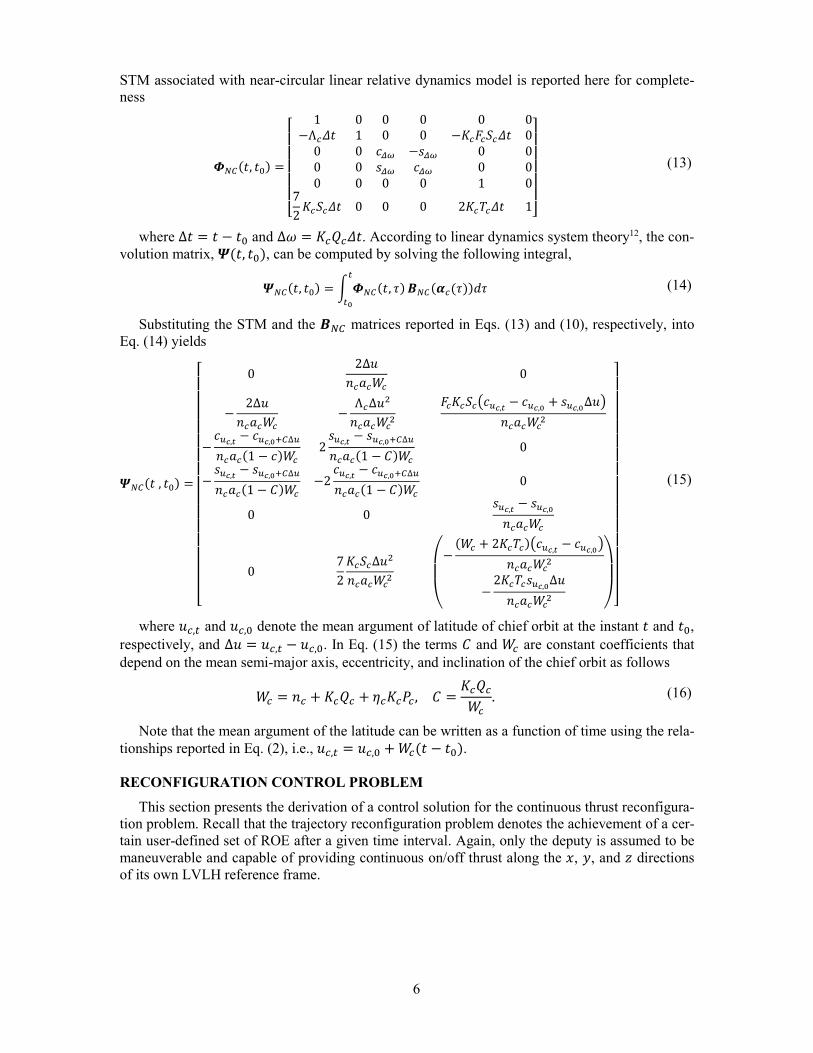
STM associated with near-circular linear relative dynamics model is reported here for complete-

ness

|pq�h, h{� =������� 1 0 0 0 0 0−Λ�~h 1 0 0 −3�s�t�~h 00 0 (�+ −%�+ 0 00 0 %�+ (�+ 0 00 0 0 0 1 072 3�t�~h 0 0 0 23�v�~h 1 !!

!!!" (13)

where Δh = h − h{ and Δ = 3�9�~h. According to linear dynamics system theory12, the con-

volution matrix, }�h, h{�, can be computed by solving the following integral,

}pq�h, h{� = � |pq�h, ����� npq�������N� (14)

Substituting the STM and the npq matrices reported in Eqs. (13) and (10), respectively, into

Eq. (14) yields

}pq�h , h{� =

����������������� 0 2∆x'����� 0

− 2∆x'����� − Λ�∆x�'������ s�3�t�G(w�,� − (w�,� + %w�,�∆xH'������− (w�,� − (w�,��q∆w'����1 − (��� 2 %w�,� − %w�,��q∆w'����1 − ���� 0− %w�,� − %w�,��q∆w'����1 − ���� −2 (w�,� − (w�,��q∆w'����1 − ���� 0

0 0 %w�,� − %w�,�'�����0 72 3�t�∆x�'������

���− ��� + 23�v��G(w�,� − (w�,�H'������

− 23�v�%w�,�∆x'������ ��� !

!!!!!!!!!!!!!!"

(15)

where x�,� and x�,{ denote the mean argument of latitude of chief orbit at the instant h and h{,

respectively, and ∆x = x�,� − x�,{. In Eq. (15) the terms � and �� are constant coefficients that

depend on the mean semi-major axis, eccentricity, and inclination of the chief orbit as follows

�� = '� + 3�9� + <�3�=� , � = 3�9��� . (16)

Note that the mean argument of the latitude can be written as a function of time using the rela-

tionships reported in Eq. (2), i.e., x�,� = x�,{ + ���h − h{�.

RECONFIGURATION CONTROL PROBLEM

This section presents the derivation of a control solution for the continuous thrust reconfigura-

tion problem. Recall that the trajectory reconfiguration problem denotes the achievement of a cer-

tain user-defined set of ROE after a given time interval. Again, only the deputy is assumed to be

maneuverable and capable of providing continuous on/off thrust along the S, T, and U directions

of its own LVLH reference frame.

7

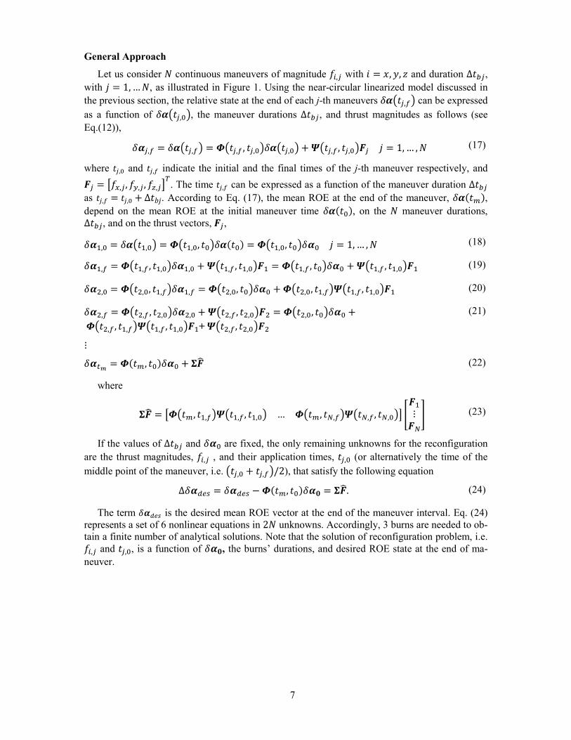
General Approach

Let us consider � continuous maneuvers of magnitude ]�,? with = S, T, U and duration ∆h�?,

with M = 1, … �, as illustrated in Figure 1. Using the near-circular linearized model discussed in

the previous section, the relative state at the end of each j-th maneuvers ��Gh?,�H can be expressed

as a function of ��Gh?,{H, the maneuver durations ∆h�?, and thrust magnitudes as follows (see

Eq.(12)), ��?,� = ��Gh?,�H = |Gh?,� , h?,{H��Gh?,{H + }Gh?,� , h?,{HW? M = 1, … , � (17)

where h?,{ and h?,� indicate the initial and the final times of the j-th maneuver respectively, and W? = \]�,?, ]�,? , ]̂ ,?_�. The time h?,� can be expressed as a function of the maneuver duration ∆h�?

as h?,� = h?,{ + ∆h�M. According to Eq. (17), the mean ROE at the end of the maneuver, ���h��,

depend on the mean ROE at the initial maneuver time ���h{�, on the � maneuver durations, ∆h�?, and on the thrust vectors, W?, ��e,{ = ��Ghe,{H = |Ghe,{, h{H���h{� = |Ghe,{, h{H��{ M = 1, … , � (18)

��e,� = |Ghe,� , he,{H��e,{ + }Ghe,� , he,{HWe = |Ghe,� , h{H��{ + }Ghe,� , he,{HWe (19)

���,{ = |Gh�,{, he,�H��e,� = |Gh�,{, h{H��{ + |Gh�,{, he,�H}Ghe,� , he,{HWe (20)

���,� = |Gh�,� , h�,{H���,{ + }Gh�,� , h�,{HW� = |Gh�,{, h{H��{ + |Gh�,� , he,�H}Ghe,� , he,{HWe+ }Gh�,�, h�,{HW� ⋮ (21)

���� = |�h�, h{���{ + �W� (22)

where

�W� = \|Gh�, he,�H}Ghe,� , he,{H … |Gh�, hp,�H}Ghp,� , hp,{H_ �We⋮Wp� (23)

If the values of ∆h�? and ��{ are fixed, the only remaining unknowns for the reconfiguration

are the thrust magnitudes, ]�,? , and their application times, h?,{ (or alternatively the time of the

middle point of the maneuver, i.e. Gh?,{ + h?,�H/2), that satisfy the following equation ∆����� = ����� − |�h�, h{���5 = �W�. (24)

The term ����� is the desired mean ROE vector at the end of the maneuver interval. Eq. (24)

represents a set of 6 nonlinear equations in 2� unknowns. Accordingly, 3 burns are needed to ob-

tain a finite number of analytical solutions. Note that the solution of reconfiguration problem, i.e. ]�,? and h?,{, is a function of ��5, the burns’ durations, and desired ROE state at the end of ma-

neuver.

8

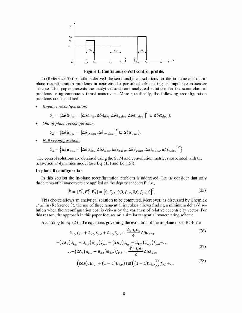
Figure 1. Continuous on/off control profile.

In (Reference 3) the authors derived the semi-analytical solutions for the in-plane and out-of

plane reconfiguration problems in near-circular perturbed orbits using an impulsive maneuver

scheme. This paper presents the analytical and semi-analytical solutions for the same class of

problems using continuous thrust maneuvers. More specifically, the following reconfiguration

problems are considered:

• In-plane reconfiguration: te = �∆�� ��� = \∆����� , ∆�#���, ∆���,���, ∆���,��� _� ⊆ ∆����� ¢; • Out-of-plane reconfiguration: t� = �∆�� ��� = \∆��,���, ∆��,��� _� ⊆ ∆����� ¢;

• Full reconfiguration: tE = £∆�� ��� = \∆�����, ∆�#���, ∆���,���, ∆���,���, ∆��,���, ∆��,���_�¤ The control solutions are obtained using the STM and convolution matrices associated with the

near-circular dynamics model (see Eq. (13) and Eq.(15)).

In-plane Reconfiguration

In this section the in-plane reconfiguration problem is addressed. Let us consider that only

three tangential maneuvers are applied on the deputy spacecraft, i.e., W� = �We� , W�� , WE� = \0, ]�,e, 0,0, ]�,�, 0,0, ]�,E, 0_� . (25)

This choice allows an analytical solution to be computed. Moreover, as discussed by Chernick

et al. in (Reference 3), the use of three tangential impulses allows finding a minimum delta-V so-

lution when the reconfiguration cost is driven by the variation of relative eccentricity vector. For

this reason, the approach in this paper focuses on a similar tangential maneuvering scheme.

According to Eq. (23), the equations governing the evolution of the in-plane mean ROE are

x¥e,�]�,e + x¥�,�]�,� + x¥E,�]�,E = ��'���4 ∆����� (26)

−G2Λ�Gx�� − x¦e,�Hx¥e,�H]�,e − G2Λ�Gx�� − x¦e,�Hx¥�,�H]�,�−. . . . . . −G2Λ�Gx�� − x¦E,�Hx¥E,�H]�,E = ���'���2 ∆�#���

(27)

§cosG�x�� + �1 − ��x¦e,�H sin §�1 − ��x¥e,�¨¨ ]�,e+. . . (28)

9

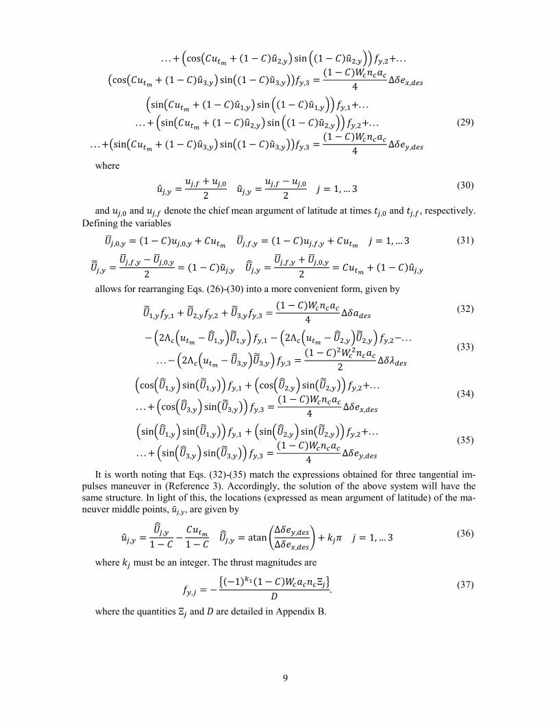
. . . + §cosG�x�� + �1 − ��x¦�,�H sin §�1 − ��x¥�,�¨¨ ]�,�+. . . GcosG�x�� + �1 − ��x¦E,�H sinG�1 − ��x¥E,�HH]�,E = �1 − ����'���4 ∆���,���

§sinG�x�� + �1 − ��x¦e,�H sin §�1 − ��x¥e,�¨¨ ]�,e+. . . . . . + §sinG�x�� + �1 − ��x¦�,�H sin §�1 − ��x¥�,�¨¨ ]�,�+. . . . . . +GsinG�x�� + �1 − ��x¦E,�H sinG�1 − ��x¥E,�HH]�,E = �1 − ����'���4 ∆���,���

(29)

where

x¦?,� = x?,� + x?,{2 x¥?,� = x?,� − x?,{2 M = 1, … 3 (30)

and x?,{ and x?,� denote the chief mean argument of latitude at times h?,{ and h?,�, respectively.

Defining the variables ©ª?,{,� = �1 − ��x?,{,� + �x�� ©ª?,�,� = �1 − ��x?,�,� + �x�� M = 1, … 3

©ª«?,� = ©ª?,�,� − ©ª?,{,�2 = �1 − ��x¥?,� ©ª�?,� = ©ª?,�,� + ©ª?,{,�2 = �x�� + �1 − ��x¦?,�

(31)

allows for rearranging Eqs. (26)-(30) into a more convenient form, given by

©ª«e,�]�,e + ©ª«�,�]�,� + ©ª«E,�]�,E = �1 − ����'���4 ∆����� (32)

− §2Λ�§x�� − ©ª�e,�¨©ª«e,�¨ ]�,e − §2Λ�§x�� − ©ª��,�¨©ª«�,�¨ ]�,�−. . . . . . − §2Λ�§x�� − ©ª�E,�¨©ª«E,�¨ ]�,E = �1 − ������'���2 ∆�#���

(33)

§cos§©ª�e,�¨ sinG©ª«e,�H¨ ]�,e + §cos§©ª��,�¨ sinG©ª«�,�H¨ ]�,�+. . . . . . + §cos§©ª�E,�¨ sinG©ª«E,�H¨ ]�,E = �1 − ����'���4 ∆���,���

(34)

§sin§©ª�e,�¨ sinG©ª«e,�H¨ ]�,e + §sin§©ª��,�¨ sinG©ª«�,�H¨ ]�,�+. . . . . . + §sin§©ª�E,�¨ sinG©ª«E,�H¨ ]�,E = �1 − ����'���4 ∆���,���

(35)

It is worth noting that Eqs. (32)-(35) match the expressions obtained for three tangential im-

pulses maneuver in (Reference 3). Accordingly, the solution of the above system will have the

same structure. In light of this, the locations (expressed as mean argument of latitude) of the ma-

neuver middle points, x¦?,�, are given by

x¦?,� = ©ª�?,�1 − � − �x��1 − � ©ª�?,� = atan f∆���,���∆���,���g + ¬?­ M = 1, … 3 (36)

where ¬? must be an integer. The thrust magnitudes are

]�,? = − ®�−1�¯°�1 − ������'�Ξ?²³ . (37)

where the quantities Ξ? and ³ are detailed in Appendix B.

10

Out-of-plane Reconfiguration

In this section the out-of-plane control solution is presented. In order to achieve the desired x

and y components of the relative inclination vector at the end of the maneuver, the control solu-

tion must include a component in the cross-track (z) direction. In fact, the only way to modify the

difference in chief and deputy orbit inclination (i.e., ��) is to provide a control action along the

z-axis of deputy LVLH frame. This is immediately evident from inspection of the linearized

equations of relative motion (see Eq. (10)). More specifically, if a single cross-track maneuver is

performed by the deputy satellite, i.e. We = \0,0, ]̂ ,e_�, the equations governing the change of in-

clination vector are (see Eq. (23))

cosGx¦e,^H sinGx¥e,^H ]̂ ,e = ��'���2 ∆��,��� (38)

´23�v�Gx�� − x¦e,^ − x¥e,^H cosGx¦e,^H sinGx¥e,^H +��� + 23�v�� sinGx¦e,^H sinGx¥e,^H−23�v� sinGx¦e,^ − x¥e,^Hx¥e,^µ ]̂ ,e = ���'���2 ∆��,��� (39)

The magnitude of the maneuver can be computed by inverting Eq. (38),

]̂ ,e = ��'���2\cosGx¦e,^H sinGx¥e,^H_ ∆��,��� (40)

The location of the maneuver, x¦e,^, can be found by substituting Eq. (40) into Eq. (39) to ob-

tain the following transcendental expression,

´23�v�Gx�� − x¦e,^ − x¥e,^H + ��� + 23�v�� tgGx¦e,^H− 23�v� sinGx¦e,^ − x¥e,^Hx¥e,^cosGx¦e,^H sinGx¥e,^H µ = �� ∆��,���∆��,��� . (41)

Eq. (41) can be numerically solved by using an iterative algorithm. The single out-of-plane

maneuver solution for unperturbed orbits provides useful insight into choosing a good initial

guess for quick convergence of the iterative approach. In this case, the location given by x¦e,^ =atan �∆��,���/∆��,���� is used.

Full Reconfiguration

In this section the solution of the full reconfiguration problem is presented. It is assumed that

no radial maneuvers are performed and that only a single maneuver is performed for the control

of the mean relative inclination vector, i.e., W� = �We� , W�� , WE� , WA� = \0, ]�,e, 0,0, ]�,�, 0,0, ]�,E, 0,0,0, ]̂ ,e_�. (42)

Then, the following set of six equations must be solved with respect to the unknowns magni-

tudes and locations, ]�,?, ]̂ ,e x¦?,� and x¦e,^ (M = 1, … 3), respectively

x¥e,�]�,e + x¥�,�]�,� + x¥E,�]�,E = ��'���4 ∆����� (43)

−G2Λ�Gx�� − x¦e,�Hx¥e,�H]�,e − G2Λ�Gx�� − x¦e,�Hx¥�,�H]�,�−. . . . . . −G2Λ�Gx�� − x¦E,�Hx¥E,�H]�,E+. . . . . . +s�3�t� f−sinGx¦e,^H sinGx¥e,^H + sinGx¦e,^ − x¥e,^Hx¥e,^ +. . .. . . +Gx�� − x¦e,^ − x¥e,^H cosGx¦e,^H sinGx¥e,^H g ]̂ ,e = ���'���2 ∆�#���

(44)

11

§cosG�x�� + �1 − ��x¦e,�H sin §�1 − ��x¥e,�¨¨ ]�,e+. . . . . . + §cosG�x�� + �1 − ��x¦�,�H sin §�1 − ��x¥�,�¨¨ ]�,�+. . . . . . +GcosG�x�� + �1 − ��x¦E,�H sinG�1 − ��x¥E,�HH]�,E = �1 − ����'���4 ∆���,���

(45)

§sinG�x�� + �1 − ��x¦e,�H sin §�1 − ��x¥e,�¨¨ ]�,e+. . . . . . + §sinG�x�� + �1 − ��x¦�,�H sin §�1 − ��x¥�,�¨¨ ]�,�+. . . . . . +GsinG�x�� + �1 − ��x¦E,�H sinG�1 − ��x¥E,�HH]�,E = �1 − ����'���4 ∆���,���

(46)

cosGx¦e,^H sinGx¥e,^H ]̂ ,e = ��'���2 ∆��,��� (47)

G73�t�Gx�� − x¦e,�Hx¥e,�H]�,e + G73�t�Gx�� − x¦�,�Hx¥�,�H]�,�+. . . … + G73�t�Gx�� − x¦E,�Hx¥E,�H]�,E+. . . . . . + ´23�v�Gx�� − x¦e,^ − x¥e,^H cosGx¦e,^H sinGx¥e,^H +. . .. . . +��� + 23�v�� sinGx¦e,^H sinGx¥e,^H +. . .. . . −23�v� sinGx¦e,^ − x¥e,^Hx¥e,^

µ ]̂ ,e = ���'���2 ∆��,���

(48)

The system (43)-(48) can be solved numerically through an iterative algorithm. The solution

results are presented in the following section. The use of analytical and semi-analytical solutions,

obtained for in-plane and out-of-plane maneuvers, as initial guess (see Eqs. (36)-(37) and Eqs.

(40)-(41)), guarantees the algorithm’s convergence in less than four iterations.

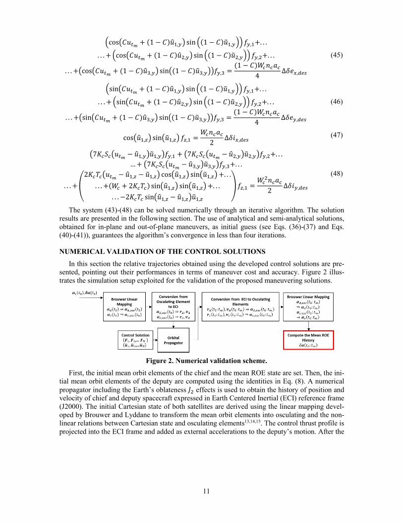
NUMERICAL VALIDATION OF THE CONTROL SOLUTIONS

In this section the relative trajectories obtained using the developed control solutions are pre-

sented, pointing out their performances in terms of maneuver cost and accuracy. Figure 2 illus-

trates the simulation setup exploited for the validation of the proposed maneuvering solutions.

Figure 2. Numerical validation scheme.

First, the initial mean orbit elements of the chief and the mean ROE state are set. Then, the ini-

tial mean orbit elements of the deputy are computed using the identities in Eq. (8). A numerical

propagator including the Earth’s oblateness �� effects is used to obtain the history of position and

velocity of chief and deputy spacecraft expressed in Earth Centered Inertial (ECI) reference frame

(J2000). The initial Cartesian state of both satellites are derived using the linear mapping devel-

oped by Brouwer and Lyddane to transform the mean orbit elements into osculating and the non-

linear relations between Cartesian state and osculating elements13,14,15. The control thrust profile is

projected into the ECI frame and added as external accelerations to the deputy’s motion. After the

12

simulation, the absolute position and velocity of the spacecraft are converted into the mean orbit

elements to compute the accuracy at the end of the maneuver, defined as ·k¸¹ = º�»¼̄w��h�� − �»¯,���º���h{� ¬ = 1, … ,6. (49)

Ultimately, a numerical optimizer is used to verify the efficiency of the proposed analytical

solutions. It is worth noting that the optimizer is only employed to check the degree to which the

analytical solution can be improved using the maneuver scheme given in Eq. (42). Hence, a de-

tailed study of the optimality of the solution as a function of the number of maneuvers is not car-

ried out in the frame of this work. More specifically, the Matlab built-in MultiStart routine is ex-

ploited to find the values of ]�,?, x¥?,� and x¦?,� with = T, U that minimize the maneuver cost in term

of ∆½ = ∑ 2]�,?x¥M,T/�( + 2]̂ ,?x¥M,U/�(p?le , satisfying the following constraints ∆����� − �W� < 1� − 8 º]�,?º < ]�Á�, x¦?�e,� > x¦?,� , ºx¥M+1,T + x¥M,Tº < ºx¦?�e,� − x¦?,�º. (50)

In the ensuing sections, we refer to the solution given by the Multistart optimizer as the numerical

solution. In order to verify the effectiveness of the designed continuous thrust maneuvers three

test cases are carried out, one for each reconfiguration problem defined in the previous sections.

Moreover, a comparison with the corresponding impulsive control scheme reported in (Reference

3) is presented for in-plane and out-of-plane reconfiguration problems.

In-plane Reconfiguration Control Problem

This section presents the trajectories obtained using the analytical control solution reported in

Eq. (36)-(37) and the numerical solution. The initial conditions used in the simulations are listed

in Table 1 and Table 2 (see first row), along with the desired mean ROE vector at the end of the

maneuver sequence. Note that the values of ��{ and ����� lead to ��∆�� ��� =��\∆�����, ∆�#���, ∆���,���, ∆���,��� _� = �−0.03, 1.9172,0.0403, 0.1198 � km.

Table 1. Initial mean chef orbit.

�� (km) �� (dim) � (deg) � (deg) ΩÄ (deg) ]� (deg)

6578 0 8 0 0 0

Table 2. Relative orbit at the initial and final maneuver time.

����

(m)

���#

(m)

�����

(m)

�����

(m)

����

(m)

����

(m)

Initial relative orbit, ��{ 30 -11e3 0 -50 0 0

Desired relative orbit, ����� 0 -10.5e3 45 70 0 0

The maneuver lasts 5 orbits, i.e. x� = 10­. The analytical solution was obtained using the

values of the maneuver intervals, ∆h�? with M = 1, … 3, and locations, ©ª�?,�, listed in Table 3. The

same table shows the maneuver cost corresponding to the numerical in-plane solution. In addi-

tion, a comparison of the continuous control solutions developed in this paper and the corre-

sponding impulsive control scheme reported in (Reference 3) is presented (see last row of Table

3). It is worth noting that the numerical continuous thrust solution requires a lower total delta-V

than the analytical method by reducing the maneuver intervals and increasing the thrust magni-

tude (see also Figure 4). Moreover, the numerical solution offers the same performance as the

corresponding analytical impulsive control solution. On the contrary, the analytical continuous

13

solution requires a higher delta-V than the impulsive scheme to achieve the desired formation

configuration. This is to be expected due to the generally lower kinematic efficiency of continu-

ous thrust maneuvering as compared with impulsive maneuvering.

Table 3. Comparison between the analytical and numerical control solution for the in-plane ma-

neuver.

Maneuver Loca-

tion, ©ª�?,� (rad)

∆Åe (km/s) / ∆h�e (min)

∆Å� (km/s) / ∆h�� (min)

∆ÅE (km/s) / ∆h�E (min)

TOT

(km/s)

Analytical

Continuous

Solution

[1.245,4.38,20.09] 0.096e-4 /

5.5

-0.466e-4 /

7.34

0.192e-4 /

7.34 7.5595e-5

Numerical

Continuous

Solution

[4.37,20.088,23.32] -0.369e-4 /

1.42

0.285e-4 /

1.80

-0.093e-4 /

0.36 7.486e-5

Analytical

Impulsive

Solution

[1.245,4.38,20.09]

0.092e-4 /

instantaneous

impulse

-0.463e-4 /

instantaneous

impulse

0.194e-4 /

instantaneous

impulse

7.48e-5

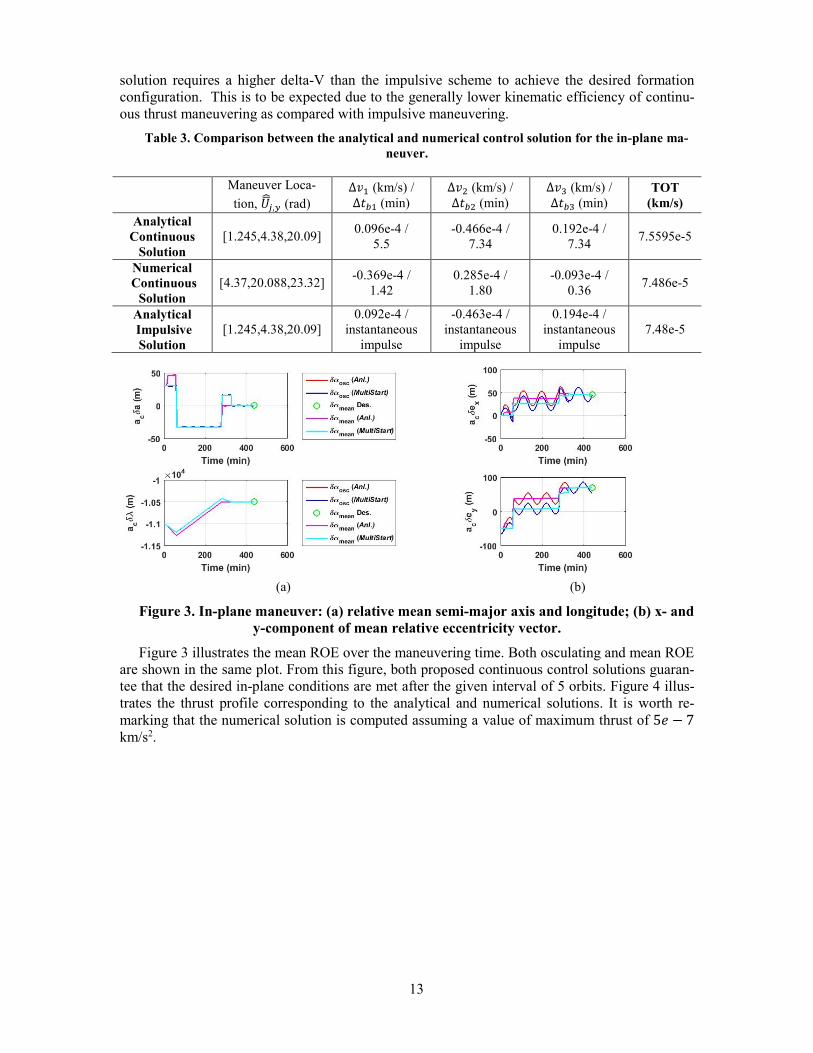
(a) (b)

Figure 3. In-plane maneuver: (a) relative mean semi-major axis and longitude; (b) x- and

y-component of mean relative eccentricity vector.

Figure 3 illustrates the mean ROE over the maneuvering time. Both osculating and mean ROE

are shown in the same plot. From this figure, both proposed continuous control solutions guaran-

tee that the desired in-plane conditions are met after the given interval of 5 orbits. Figure 4 illus-

trates the thrust profile corresponding to the analytical and numerical solutions. It is worth re-

marking that the numerical solution is computed assuming a value of maximum thrust of 5� − 7

km/s2.

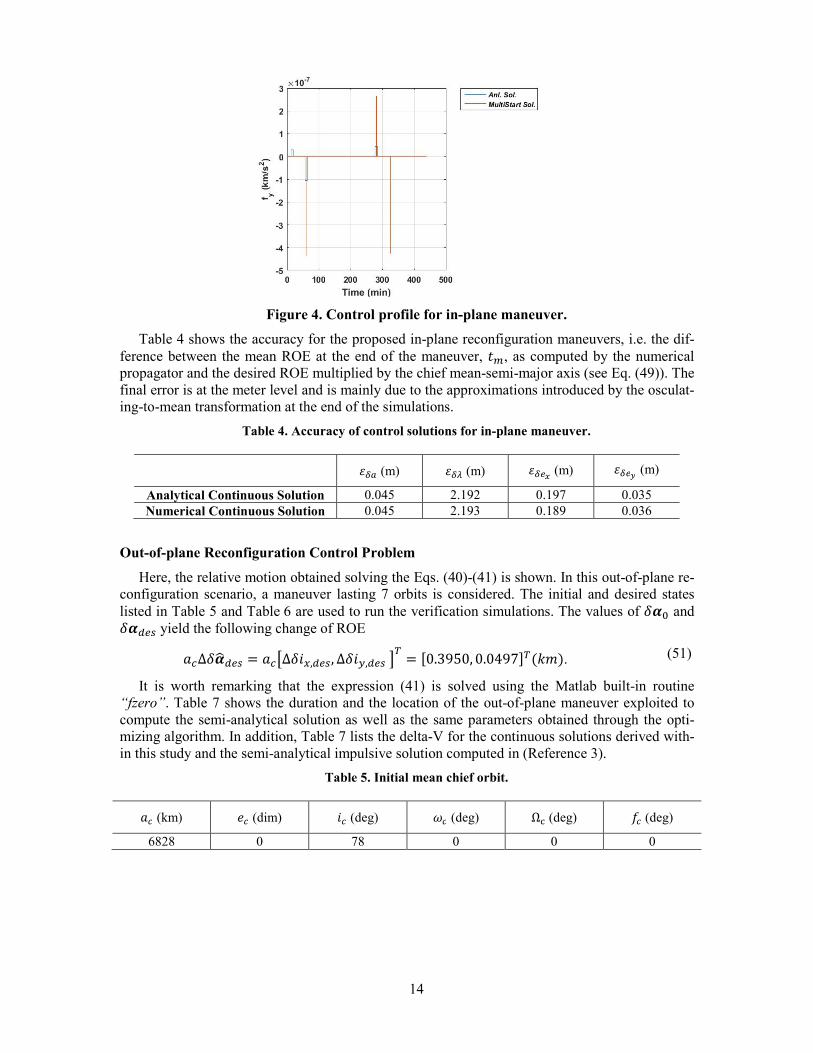
14

Figure 4. Control profile for in-plane maneuver.

Table 4 shows the accuracy for the proposed in-plane reconfiguration maneuvers, i.e. the dif-

ference between the mean ROE at the end of the maneuver, h�, as computed by the numerical

propagator and the desired ROE multiplied by the chief mean-semi-major axis (see Eq. (49)). The

final error is at the meter level and is mainly due to the approximations introduced by the osculat-

ing-to-mean transformation at the end of the simulations.

Table 4. Accuracy of control solutions for in-plane maneuver.

·kÁ (m) ·kÆ (m) ·k�Ç (m) ·k�È (m)

Analytical Continuous Solution 0.045 2.192 0.197 0.035

Numerical Continuous Solution 0.045 2.193 0.189 0.036

Out-of-plane Reconfiguration Control Problem

Here, the relative motion obtained solving the Eqs. (40)-(41) is shown. In this out-of-plane re-

configuration scenario, a maneuver lasting 7 orbits is considered. The initial and desired states

listed in Table 5 and Table 6 are used to run the verification simulations. The values of ��{ and ����� yield the following change of ROE ��∆�� ��� = ��\∆��,���, ∆��,��� _� = �0.3950, 0.0497 ��¬É�. (51)

It is worth remarking that the expression (41) is solved using the Matlab built-in routine

“fzero”. Table 7 shows the duration and the location of the out-of-plane maneuver exploited to

compute the semi-analytical solution as well as the same parameters obtained through the opti-

mizing algorithm. In addition, Table 7 lists the delta-V for the continuous solutions derived with-

in this study and the semi-analytical impulsive solution computed in (Reference 3).

Table 5. Initial mean chief orbit.

�� (km) �� (dim) � (deg) � (deg) ΩÄ (deg) ]� (deg)

6828 0 78 0 0 0

15

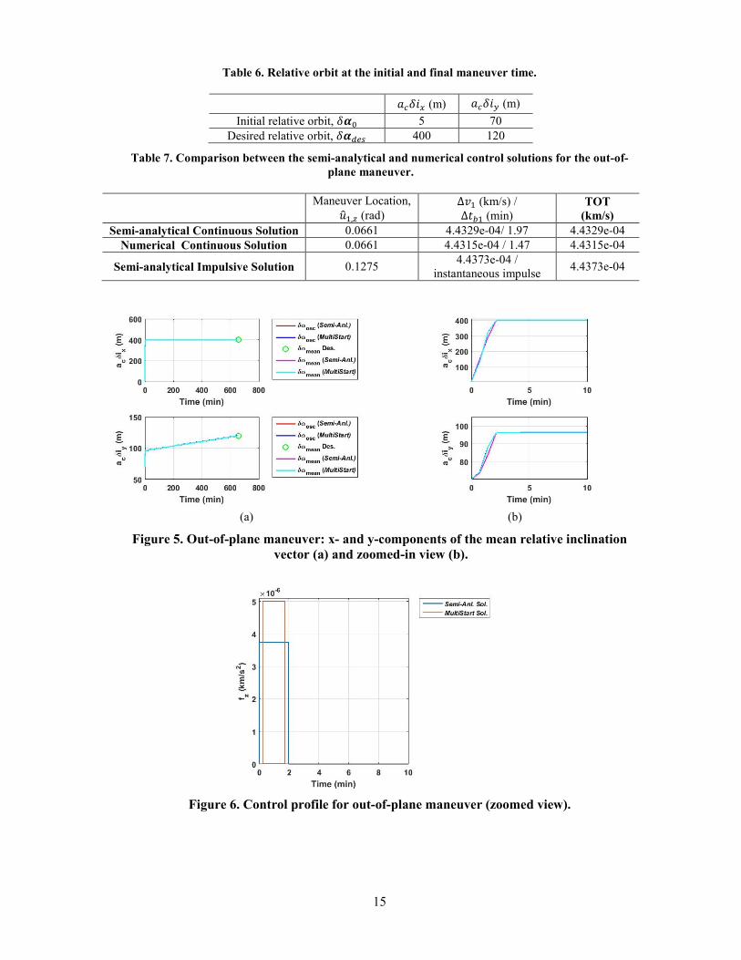
Table 6. Relative orbit at the initial and final maneuver time.

���� (m) ���� (m)

Initial relative orbit, ��{ 5 70

Desired relative orbit, ����� 400 120

Table 7. Comparison between the semi-analytical and numerical control solutions for the out-of-

plane maneuver.

Maneuver Location, x¦e,^ (rad)

∆Åe (km/s) / ∆h�e (min)

TOT

(km/s)

Semi-analytical Continuous Solution 0.0661 4.4329e-04/ 1.97 4.4329e-04

Numerical Continuous Solution 0.0661 4.4315e-04 / 1.47 4.4315e-04

Semi-analytical Impulsive Solution 0.1275 4.4373e-04 /

instantaneous impulse 4.4373e-04

(a) (b)

Figure 5. Out-of-plane maneuver: x- and y-components of the mean relative inclination

vector (a) and zoomed-in view (b).

Figure 6. Control profile for out-of-plane maneuver (zoomed view).

16

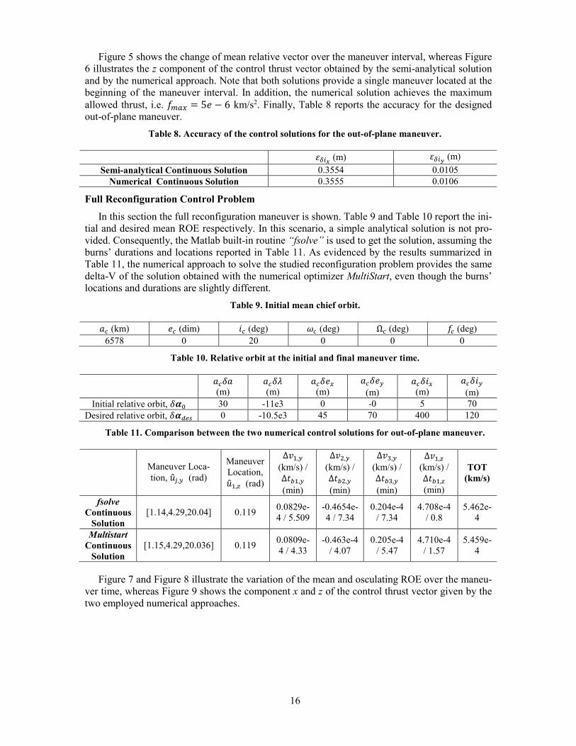
Figure 5 shows the change of mean relative vector over the maneuver interval, whereas Figure

6 illustrates the z component of the control thrust vector obtained by the semi-analytical solution

and by the numerical approach. Note that both solutions provide a single maneuver located at the

beginning of the maneuver interval. In addition, the numerical solution achieves the maximum

allowed thrust, i.e. ]�Á� = 5� − 6 km/s2. Finally, Table 8 reports the accuracy for the designed

out-of-plane maneuver.

Table 8. Accuracy of the control solutions for the out-of-plane maneuver.

·k�Ç (m) ·k�È (m)

Semi-analytical Continuous Solution 0.3554 0.0105

Numerical Continuous Solution 0.3555 0.0106

Full Reconfiguration Control Problem

In this section the full reconfiguration maneuver is shown. Table 9 and Table 10 report the ini-

tial and desired mean ROE respectively. In this scenario, a simple analytical solution is not pro-

vided. Consequently, the Matlab built-in routine “fsolve” is used to get the solution, assuming the

burns’ durations and locations reported in Table 11. As evidenced by the results summarized in

Table 11, the numerical approach to solve the studied reconfiguration problem provides the same

delta-V of the solution obtained with the numerical optimizer MultiStart, even though the burns’

locations and durations are slightly different.

Table 9. Initial mean chief orbit.

�� (km) �� (dim) � (deg) � (deg) ΩÄ (deg) ]� (deg)

6578 0 20 0 0 0

Table 10. Relative orbit at the initial and final maneuver time.

���� (m)

���# (m)

����� (m)

�����

(m)

���� (m)

����

(m)

Initial relative orbit, ��{ 30 -11e3 0 -0 5 70

Desired relative orbit, ����� 0 -10.5e3 45 70 400 120

Table 11. Comparison between the two numerical control solutions for out-of-plane maneuver.

Maneuver Loca-

tion, x¦?,� (rad)

Maneuver

Location, x¦e,^ (rad)

∆Åe,�

(km/s) / ∆h�e,�

(min)

∆Å�,�

(km/s) / ∆h��,�

(min)

∆ÅE,�

(km/s) / ∆h�E,�

(min)

Ɓe,^

(km/s) / ∆h�e,^

(min)

TOT

(km/s)

fsolve

Continuous

Solution

[1.14,4.29,20.04] 0.119 0.0829e-

4 / 5.509

-0.4654e-

4 / 7.34

0.204e-4

/ 7.34

4.708e-4

/ 0.8

5.462e-

4

Multistart

Continuous

Solution

[1.15,4.29,20.036] 0.119 0.0809e-

4 / 4.33

-0.463e-4

/ 4.07

0.205e-4

/ 5.47

4.710e-4

/ 1.57

5.459e-

4

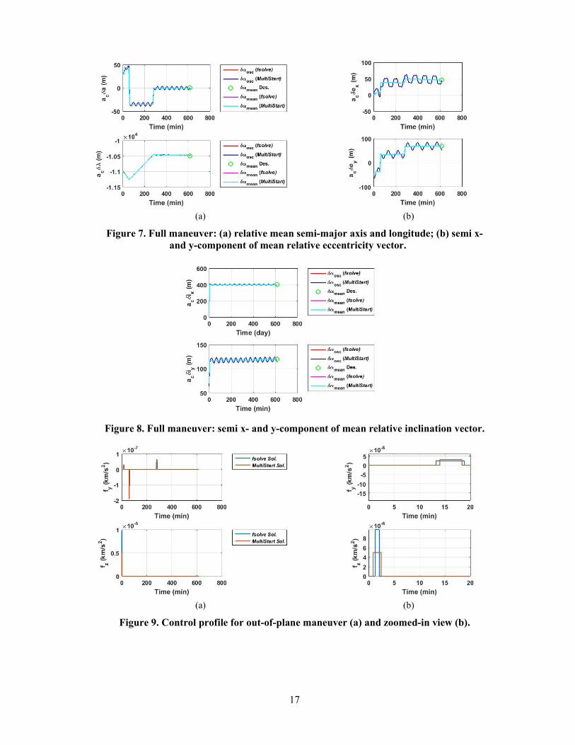
Figure 7 and Figure 8 illustrate the variation of the mean and osculating ROE over the maneu-

ver time, whereas Figure 9 shows the component x and z of the control thrust vector given by the

two employed numerical approaches.

17

(a) (b)

Figure 7. Full maneuver: (a) relative mean semi-major axis and longitude; (b) semi x-

and y-component of mean relative eccentricity vector.

Figure 8. Full maneuver: semi x- and y-component of mean relative inclination vector.

(a) (b)

Figure 9. Control profile for out-of-plane maneuver (a) and zoomed-in view (b).

18

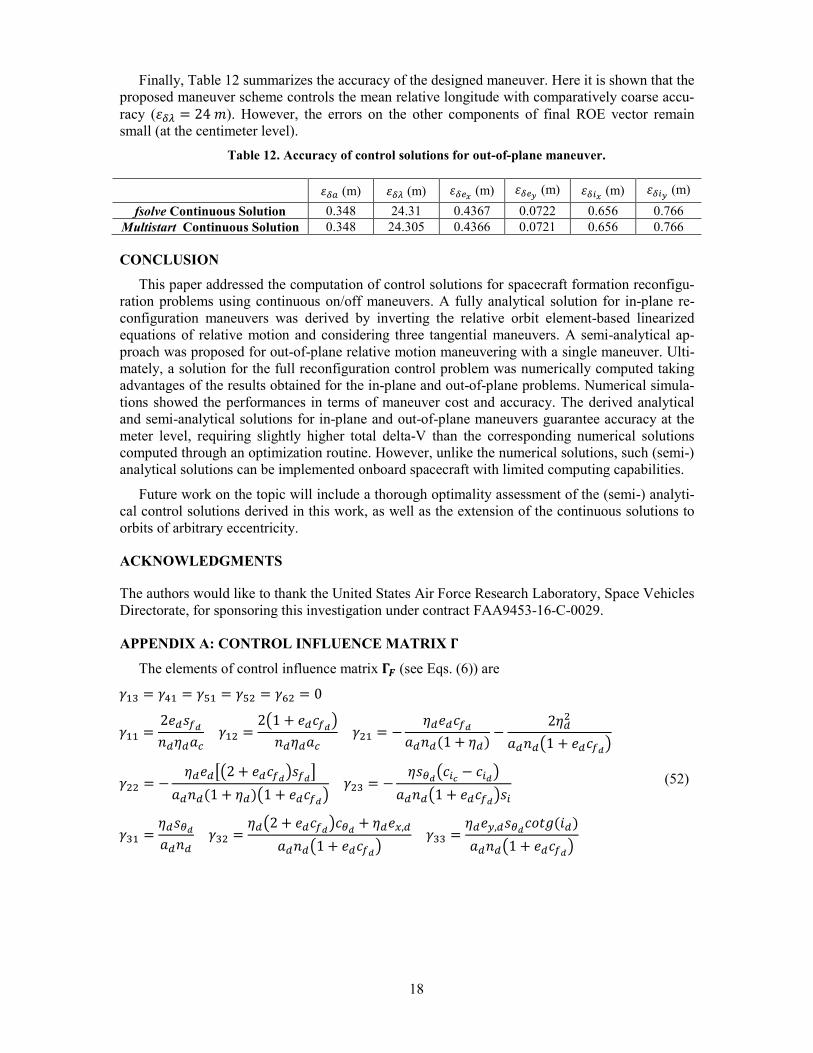
Finally, Table 12 summarizes the accuracy of the designed maneuver. Here it is shown that the

proposed maneuver scheme controls the mean relative longitude with comparatively coarse accu-

racy (·kÆ = 24 É). However, the errors on the other components of final ROE vector remain

small (at the centimeter level).

Table 12. Accuracy of control solutions for out-of-plane maneuver.

·kÁ (m) ·kÆ (m) ·k�Ç (m) ·k�È (m) ·k�Ç (m) ·k�È (m)

fsolve Continuous Solution 0.348 24.31 0.4367 0.0722 0.656 0.766

Multistart Continuous Solution 0.348 24.305 0.4366 0.0721 0.656 0.766

CONCLUSION

This paper addressed the computation of control solutions for spacecraft formation reconfigu-

ration problems using continuous on/off maneuvers. A fully analytical solution for in-plane re-

configuration maneuvers was derived by inverting the relative orbit element-based linearized

equations of relative motion and considering three tangential maneuvers. A semi-analytical ap-

proach was proposed for out-of-plane relative motion maneuvering with a single maneuver. Ulti-

mately, a solution for the full reconfiguration control problem was numerically computed taking

advantages of the results obtained for the in-plane and out-of-plane problems. Numerical simula-

tions showed the performances in terms of maneuver cost and accuracy. The derived analytical

and semi-analytical solutions for in-plane and out-of-plane maneuvers guarantee accuracy at the

meter level, requiring slightly higher total delta-V than the corresponding numerical solutions

computed through an optimization routine. However, unlike the numerical solutions, such (semi-)

analytical solutions can be implemented onboard spacecraft with limited computing capabilities.

Future work on the topic will include a thorough optimality assessment of the (semi-) analyti-

cal control solutions derived in this work, as well as the extension of the continuous solutions to

orbits of arbitrary eccentricity.

ACKNOWLEDGMENTS

The authors would like to thank the United States Air Force Research Laboratory, Space Vehicles

Directorate, for sponsoring this investigation under contract FAA9453-16-C-0029.

APPENDIX A: CONTROL INFLUENCE MATRIX [

The elements of control influence matrix [W (see Eqs. (6)) are @eE = @Ae = @Êe = @Ê� = @Ë� = 0

@ee = 2��%�O'�<��� @e� = 2G1 + ��(�OH'�<��� @�e = − <���(�O��'��1 + <�� − 2<����'�G1 + ��(�OH

@�� = − <���\G2 + ��(�OH%�O_��'��1 + <��G1 + ��(�OH @�E = − <%ÌOG(�� − (�OH��'�G1 + ��(�OH%� @Ee = <�%ÌO��'� @E� = <�G2 + ��(�OH(ÌO + <���,���'�G1 + ��(�OH @EE = <���,�%ÌO()hÍ�����'�G1 + ��(�OH

(52)

19

@Ae = − <�(ÌO��'� , @A� = <�G2 + ��(�OH%ÌO + <���,���'�G1 + ��(�OH

@AE = − <���,�%ÌO()hÍ�����'�G1 + ��(�OH @ÊE = <�%ÌO��'�G1 + ��(�OH @ËE = <�(ÌO%����'�G1 + ��(�OH%�O

where ]� and Î� represent the deputy satellite’s true anomaly and true argument of latitude re-

spectively.

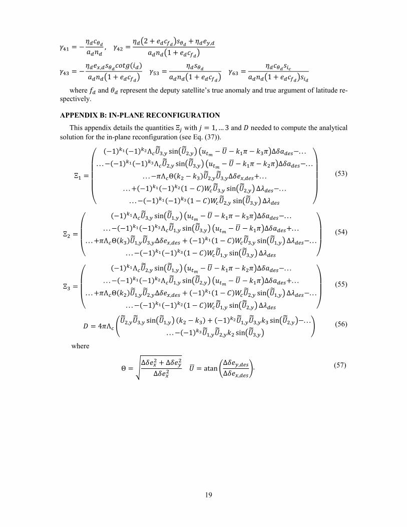
APPENDIX B: IN-PLANE RECONFIGURATION

This appendix details the quantities Ξ? with M = 1, … 3 and ³ needed to compute the analytical

solution for the in-plane reconfiguration (see Eq. (37)).

Ξe =����� �−1�¯°�−1�¯ÏΛ�©ª«E,� sinG©ª«�,�H Gx�� − ©ª − ¬e­ − ¬E­H∆�����−. . .. . . −�−1�¯°�−1�¯ÐΛ�©ª«�,� sinG©ª«E,�H Gx�� − ©ª − ¬e­ − ¬�­H∆�����−. . .. . . −­Λ�Θ�¬� − ¬E�©ª«�,�©ª«E,�∆���,���+. . .. . . +�−1�¯°�−1�¯Ï�1 − ����©ª«E,� sinG©ª«�,�H ∆#���−. . .. . . −�−1�¯°�−1�¯Ð�1 − ����©ª«�,� sinG©ª«E,�H ∆#��� �

����

(53)

� =����

�−1�¯°Λ�©ª«E,� sinG©ª«e,�H Gx�� − ©ª − ¬e­ − ¬E­H∆�����−. . .. . . −�−1�¯°�−1�¯ÐΛ�©ª«e,� sinG©ª«E,�H Gx�� − ©ª − ¬e­H∆�����+. . .. . . +­Λ�Θ�¬E�©ª«e,�©ª«E,�∆���,��� + �−1�¯°�1 − ����©ª«E,� sinG©ª«e,�H ∆#���−. . .. . . −�−1�¯°�−1�¯Ð�1 − ����©ª«e,� sinG©ª«E,�H ∆#��� ���� (54)

ΞE =����

�−1�¯°Λ�©ª«�,� sinG©ª«e,�H Gx�� − ©ª − ¬e­ − ¬�­H∆�����−. . .. . . −�−1�¯°�−1�¯ÏΛ�©ª«e,� sinG©ª«�,�H Gx�� − ©ª − ¬e­H∆�����+. . .. . . +­Λ�Θ�¬��©ª«e,�©ª«�,�∆���,��� + �−1�¯°�1 − ����©ª«�,� sinG©ª«e,�H ∆#���−. . .. . . −�−1�¯°�−1�¯Ï�1 − ����©ª«e,� sinG©ª«�,�H ∆#��� ���� (55)

³ = 4­Λ� Ò©ª«�,�©ª«E,� sinG©ª«e,�H �¬� − ¬E� + �−1�¯Ï©ª«e,�©ª«E,�¬E sinG©ª«�,�H−. . .. . . −�−1�¯Ð©ª«e,�©ª«�,�¬� sinG©ª«E,�H Ó (56)

where

Θ = C∆���� + ∆����∆���� ©ª = atan f∆���,���∆���,���g. (57)

20

REFERENCES

1 S.S. Vaddi, K.T. Alfriend, S.R. Vadali, et al., “Formation establishment and reconfiguration using impulsive control”.

Journal of Guidance, Control, and Dynamics. Vol. 28, No. 2, 2005, pp. 262–268, DOI: 10.2514/1.6687.

2 Y. Ichimura, A. Ichikawa, “Optimal impulsive relative orbit transfer along a circular orbit”. Journal of Guidance,

Control, and Dynamics. Vol. 31, No. 4, 2008, pp. 1014–1027, DOI: 10.2514/1.32820.

3 M. Chernick, S. D’Amico, “New Closed-Form Solutions for Optimal Impulsive Control of Spacecraft Relative Mo-

tion”. AIAA Space and Astronautics Form and Exposition, SPACE 2016, Long Beach Convention Center California,

13-16 September, 2016.

4 M. Lawn, G. Di Mauro and R. Bevilacqua, "Guidance solutions for Spacecraft Planar Rephasing and Rendezvous

using Input Shaping Control". 27th AAS/AIAA Space Flight Mechanics Meeting, San Antonio, 2017.

5L. Steindorf, S. D’Amico, J. Scharnagl, F. Kempf, K. Schilling, “Constrained Low-Thrust Satellite Formation-Flying

using Relative Orbit Elements”. 27th AAS/AIAA Space Flight Mechanics Meeting, San Antonio, Texas, February 5-9,

2017.

6 Koenig, A.W., Guffanti, T. and D'Amico, S., "New State Transition Matrices for Relative Motion of Spacecraft

Formations in Perturbed Orbits," AIAA/AAS Astrodynamics Specialist Conference, SPACE Conference and Exposition,

AIAA, 2016, DOI: 10.2514/6.2016-5635.

7 D'Amico, S., "Autonomous Formation Flying in Low Earth Orbit," Ph.D. Dissertation, University of Delft, Delft,

Netherlands, 2010.

8 S. D'Amico, "Relative Orbital Elements as Integration Constants of Hill’s Equations," DLR-GNSOC TN 05-08,

Oberpfaffenhofen, 2005.

9 Roscoe, C.W. T., Westphal, J.J., Griesbach, J.D., and Schaub H., "Formation Establishment and Reconfiguration Us-

ing Differential Elements in J2-Perturbed Orbits", Journal of Guidance, Control, and Dynamics, Vol. 38, pp. 1725-

1740, 2015, DOI: 10.2514/1.G000999.

10 Schaub, H. and Junkins, J. L., Analytical Mechanics of Space Systems, AIAA, Reston, Virginia (USA), 2014, Chap.

14

11 J. Sullivan, A. W. Koening and S. D'Amico, "Improved MAneuver Free Approach Angles-Only Navigation for

Space Rendezvous," Advances in the Astronautical Sciences Spaceflight Mechanics, vol. 158, 2016.

12 Crassidis and J. L. Junkins, Optimal Estimation of Dynamic Systems, CRC Press, 2004.

13 D. Brouwer, "Solution of the Problem of Artificial Satellite Theory Without Drag," Astronautical Journal, vol. 64,

no. 1274, 1959, pp. 378-397.

14 R. Lyddane, "Small Eccentricities or Inclinations in the Brouwer Theory of the," Astronomical Journal, vol. 68, no.

8, 1963, pp. 555-558.

15 Vallado, D.A., Fundamentals of Astrodynamics and Applications, Springer-Verlag New York, 2007.