itls-wp-07-08 - the university of sydney business school

I T L S

INSTITUTE of TRANSPORT and LOGISTICS STUDIES The Australian Key Centre in Transport and Logistics Management

The University of Sydney Established under the Australian Research Council’s Key Centre Program.

WORKING PAPER ITLS-WP-07-08 Climate Change, Enhanced Greenhouse Gas Emissions and Passenger Transport – What can we do to make a difference? By David A Hensher May 2007 ISSN 1832-570X

NUMBER: Working Paper ITLS-WP-07-08 TITLE: Climate Change, Enhanced Greenhouse Gas Emissions and

Passenger Transport – What can we do to make a difference? ABSTRACT: Climate change, global warming and enhanced greenhouse gas emissions

(GGEs) are hot topics for many reasons, including scientific and speculative. The transportation sector, led by the automobile, has been cited constantly as a major contributor through human intervention to climate change. The media and lobby groups have, for many years escalated the case for finding ways to reduce the impact that people movement has on enhanced GGEs. Governments have ramped up the rhetoric to gain political support. Short of banning car use, the challenge remains one of understanding better what mix of actions might contribute in non-marginal ways to reducing the growth of GGEs (primarily CO2) and even reduce the absolute amount of CO2 produced by automobility. This paper evaluates potentially effective instruments that are aimed at a number of policy objectives linked to the triple bottom line – efficiency, sustainability and equity – focussing on social surplus gains in addition to cost effectiveness; but in particular the ability to reduce CO2. We use TRESIS, an integrated transport, land use and environmental strategy impact simulation program, developed by the author, to assess the influence on CO2 of a number of ‘at source’ and ‘mitigation’ instruments such as improvements in fuel efficiency, a carbon tax, congestion charging, variable user charges, and improvements in public transit. We apply TRESIS to the Sydney metropolitan area with instruments enacted in 2010 up to 2015. There are some instruments that can reduce CO2 in the passenger transport sector by 5 percent over the next 8 years, with some more politically palatable, although requiring a greater amount of investment outlay by government. A mix of technological improvement linked to fuel efficiency and pricing of car use offer the most balanced way forward in terms of impacts on all stakeholders, especially in preserving government revenue sources and the opportunity to re-invest back into the transport sector through improved multi-modal infrastructure.

KEY WORDS: Greenhouse Gas Emissions, Passenger Transport, CO2, Tresis1.4,

Systemwide Impacts, Strategic Prioritization, Variable User Charges, Carbon Tax, Congestion Charges

AUTHOR: David A Hensher CONTACT: Institute of Transport and Logistics Studies (C37) An Australian Key Centre The University of Sydney NSW 2006 Australia Telephone: +61 9351 0071 Facsimile: +61 9351 0088 E-mail: [email protected] Internet: http://www.itls.usyd.edu.au DATE: May 2007 Acknowledgments. The comments by Alastair Stone (Chair ITLS Board of Advice) are greatly appreciated. I also thank John Stanley for encouraging me to bring back TRESIS as a powerful framework within which to investigate policy instruments that are capable of influencing change.

mailto:[email protected]

Climate Change, Enhanced Greenhouse Gas Emissions and Passenger Transport – What can we do to make a difference?

Hensher

1. Introduction Transport accounts for 14 percent of global greenhouse gas emissions, with the vast majority of these emissions produced by the road transport sector, passenger and freight. In the Australian context transport contributed, in 2004, 76.2 Mt CO2-e (megatonnes of carbon dioxide equivalent) or 13.5 percent of Australia’s net emissions. After the stationary energy sector, transport is the second largest growth sector in GGEs over the 1990 to 2004 period, with an increase of 23.4 percent (14.5 Mt CO2-e) (ABS 2007), or about 1.5 percent annually. The strongest period of growth in transport emissions occurred in the early 1990s and since that time the longer term growth rate appears to have slowed. The main driver for the increase in transport emissions is the continuing growth in household incomes and number of vehicles. Passenger cars were the largest transport source, contributing 41.7 Mt. CO2-e, increasing by 18 percent between 1990 and 2004, well above total net emissions growth of 5.2 percent. This represents, in 2004, 7.8 percent of Australia’s GGEs, up from 7.0 percent in 1990. The growth in emissions from passenger cars reflects growth in activity but also the influence of technological change, as the proportion of vehicles fitted with three way catalytic converters has increased in the overall passenger car fleet1. The ECMT (2007) review of progress in ECMT and OECD countries suggests that measures adopted to date in the transport sector (all modes) might cut 700 million tonnes from annual CO2 emissions by 2010, approximately 50 percent of the projected increase in emissions between 1990 and 2010. Road transport is currently the dominant modal sector in contributing to total CO2 emissions, with road passenger modes accounting for close to two-thirds of total emissions in 2030, with the road freight sector growing at a faster rate. With potential substitution of hydrogen for fossil fuels, the possibility that the road transport sector reduces its relative contribution to total CO2 is real, with aviation and maritime growing disproportionately. The UK Stern report (Stern 2006, p. xi) argues that To stabilise at 450ppm CO2e, without overshooting, global emissions would need to peak in the next 10 years and then fall at more than 5% per year, reaching 70% below current levels by 2050. Achieving major reductions in GGEs in the road passenger transport sector is not beyond the realms of possibility, as shown in the assessment of a number of instruments that can make a difference if adopted by government (ECMT 2007). Reducing GGEs however must be assessed in the context of cost effectiveness. There are a number of possible ways of reducing CO2 that deliver equivalent reductions; however some impose greater costs of society than other policy instruments. Examples include variable user charges, congestion charging and a carbon tax (see below), but the change in consumer surplus and total end

1 Catalytic converters, introduced for local air pollution control, reduce all NOx emissions but raise nitrous oxide (N2O) emissions compared with other technologies.

1

Climate Change, Enhanced Greenhouse Gas Emissions and Passenger Transport – What can we do to make a difference? Hensher user money and time costs are likely to be substantially different, as are the revenue implications for government. Importantly, the assessment of the overall impact of any policy instrument or mixes of instruments must be established through a framework that can account for the systemwide responses and not the obvious direct (partial) responses. Although there will be adjustments beyond the transport sector, there is great merit in tracking the ways in which specific policy instruments impact, in direct and indirect ways, on activities that are linked to transportation and location decisions for the population of interest. To understand how a systemwide approach can identify the impact of a specific policy instrument, consider a fuel tax increase. The imposition of an increase in the tax on automobile fuel, via its impact on unit operating cost has an immediate and direct influence on (i) the use of each vehicle for particular trips such as the commuter trip; i.e. mode choice, which includes both a switch to public transport and vehicle-substitution from within the household’s vehicle park, (ii) a change in the timing of the commuter journey to reduce the increased costs associated with traffic congestion, and hence (iii) a change in the overall and non-commuting use of each automobile available to a household. It also directly affects the household’s choice of types of automobiles from the set of conventional and hybrid-fuel vehicles. The indirect impacts include a change in residential location over time via the change in modal and spatial accessibility to work opportunities and a change in the number of vehicles in a household (given the increased operating costs). Changes in residential location may further affect the total use of each automobile, as well as the mix of urban commuting and non-commuting, and non-urban kilometres. The adjustment in commuter travel may also affect non-commuting car use if a vehicle previously used for commuting is released for use by another non-working member of the household. Some adjustment in the loss rate of automobiles will also occur. The response paths are summarised in Figure 1. This paper evaluates potentially effective instruments that are aimed at a number of policy objectives linked to the triple bottom line – efficiency, sustainability and equity; but in particular the ability to reduce CO2. We use TRESIS, an integrated transport, land use and environmental strategy impact simulation program to assess the influence on CO2 of a number of instruments such as a carbon tax, variable user charges, congestion charging, fuel efficiency gains and improvements in public transit. We apply TRESIS to the Sydney metropolitan area with instruments enacted in 2010 up to 2015. The paper is organised as follows. We begin with an overview of TRESIS1.4, an enhanced version of the program (version 1.1) presented in Hensher (2002) and Hensher and Ton (2002), followed by a case study in which we select a number of policy instruments that the literature suggests offer the greatest possibilities of reducing GGEs. The next section presents the key findings in terms of CO2 but also other crucial indicators of performance in terms of efficiency, equity and sustainability such as aggregate consumer surplus. We conclude with suggestions for ongoing research efforts.

2


Hensher

Tracing the Impact of a Fuel Tax

Household ResidentialLocation Choice

Household AutomobileFleet Size Choice

Household AutomobileType Choice

Use of Each HouseholdAutomobile (vkm)

Commuter ModeChoice

Commuter DepartureTime Choice

Workplace LocationChoice

LocationRents(HousePrices)

UsedAutomobilePrices

CommutingTravelTimes

HouseholdNon-CommutingAutomobile Useby Each Vehicle

commutingaccessibilityindex

Unit Fuel Cost(c/vkm)

auto type choiceinclusivevalue

Exogenous Shock:fuel tax increase

1

1

1

Codes: 1 = direct influence via the exogenous variable defining the shock (strategy)2 = indirect traceable impact

1

3 = intervening calculation

32

2

3

13

2

Other linkages in the overall model system

3

2

3

dwelling typechoice inclusivevalue

2

IV

2

2

2

Figure 1: Tracing the Impact of a Policy Instrument

2. Overview of TRESIS TRESIS2 ((Transportation and Environment Strategy Impact Simulator) is designed as a policy advisory tool to evaluate the impact of transport and non-transport policy instruments on urban travel behaviour and the environment with a wide range of performance indicators. As an integrated model TRESIS1.4 offers users the ability to analyse and evaluate a variety of land use, transport, and environmental policy strategies or scenarios for urban areas. The results of a base case scenario are used as references to compare with those of the policies and projects to be tested. The model generates a number of performance indicators to evaluate these effects in terms of economic, social, environmental and energy impacts. Earlier versions of TRESIS (with a 1993 base year) have been developed and applied to six Australian cities, namely Canberra, Sydney, Melbourne, Brisbane, Adelaide and Perth (Hensher et al. 1995, 2005, Hensher 2002). The latest version of TRESIS, modified and enhanced (with a 1998 base year), examines strategic level policy options for the Sydney Metropolitan Area (including the Central Coast). TRESIS1.4 has a high temporal resolution with an annual step-up to a 28-year forecasting horizon (i.e., to 2025). It has integration of land use and transport interaction in each

2 Developed since 1995at the Institute of Transport and Logistics Studies (ITLS), the University of Sydney.

3

Climate Change, Enhanced Greenhouse Gas Emissions and Passenger Transport – What can we do to make a difference? Hensher simulation period. The synthetic nature of the model provides a detailed description of the base year of 1998 to be estimated within the model. TRESIS1.4 is structured around seven key systems (see Figure 2).

Behavioral-Based Demand Specification

System

Policy Specification System

Behavioral-Based Demand Evaluation

System

Supply System

Demand/Supply Interaction System

Reporting System

Simulation Specification System

Figure 2: TRESIS1.4 Structure Behavioural demand specification system. This core system provides the household characteristics data and model formulation for the behavioural demand evaluation system. It contains a module for constructing a synthetic household database as well as a suite of utility expressions representing a behavioural system of choice models for individuals and households. These models are based on mixtures of revealed and stated preference data and estimated as an interlinked set of nested logit models (Table 1 and Figure 3) for residential location choice, dwelling type choice, mode choice, trip timing, work place location, vehicle choice type, fleet size, and automobile use by location. Each synthetic household carries a weight that represents its contribution to the total population of households defined by a set of socioeconomic characteristics of each person in the household and the household as a whole. TRESIS1.4 carries forward in time the base year household weights or, alternatively, modifies the weights to represent the changing composition of households in the population. More detail information on the specification

4


Hensher

and procedure for the generation of synthetic households to represent population data is given in Ton and Hensher (2001). The key matrices used to establish the location and travel demands for the population as a whole (given below) are derived from an accumulation of inter-related impacts across the full set of location, travel and vehicle choices made by synthetic household, each of which represents a particular socio-demographic profile of persons who define households.

, ,1

nh

rLoc dwt h h rLoc h rLoc dwth

DDMatrix weight x pRLC x pDwTC=

=∑

, ,

1,,,,,

1 1 1,

VDMatrix ∑∑∑∑= = = =

=nh

hvshfrLochrLochh

nf

f

ns

s

nv

vhSociorLoc pATCxpFSCxpRLCxweight

, , ,mod , , , , , , , , , ,mod1 1

nh nw

tod rLoc wLoc e hSocio h h rLoc h w rLoc wLoc h w tod rLoc wLoc eh w

TMatrix weight x pRLC x pWLC x pDTCMC= =

=∑∑where:

• DDMatrix rLoc,dwt = estimated number of dwellings of type dwt in zone rLoc • VDMatrixrLoc,hSocio = estimated number of vehicles from residential zone rLoc and

household type hSocio • TMatrix tod,rLoc,wLoc,mode,hSocio = estimated number of passenger trips generated by

household type hSocio at time of day tod from residential zone rLoc to destination zone wLoc by transport mode mode. The matrix of total trips can be estimated by multiplying every TMatrix cell with an expansion factor matrix cell (tod,mode,rLoc,wLoc).

• pRLC h,rLoc = residential location choice probability of household h for zone rLoc • pDwTC h,rLoc,dwt = dwelling type choice probability of household h for zone rLoc and

dwelling type dwt • pRLCh,rLoc = residential location choice probability of household h for zone rLoc • pFSCh,rLoc,f = vehicle fleet size choice probability of household h for zone rLoc and

fleet size f • pATCh,s,v = automobile technology type choice probability of household h for vehicle

size s and vintage v • w = worker (w ranges from 1 to nw) • pRLCh,rLoc = residential location choice probability of household h for zone rLoc • pWLC h,w,rLoc,wLoc = work place location choice probability of worker w in household h

for residential zone rLoc and destination zone wLoc • pDTCMCh,w,tod,rLoc,wLoc,mode = departure time and mode choice probability of worker w

in household h for residential zone rLoc and destination zone wLoc at time of day tod and transport mode mode

• h = household h (h ranges from 1 to nh) • weighth = weight of household h

5

Climate Change, Enhanced Greenhouse Gas Emissions and Passenger Transport – What can we do to make a difference? Hensher

Table 1: Classification of Key Input Data used by Choice Models in TRESIS1.4

Specific Model Choice Set Key Attributes Specific Location

Application

Relevance

Residential Location Choice (RLC)

No. of residential zones

Zone Data (distance to CBD); Accessibility measured by DwTC and WLC models

Origin Spatial, Social, Economic

Dwelling Type Choice (DwTC)

No. of dwelling types

Household Socio-economic Data; (household type, household income, number of workers); Zone Data (distance to CBD, dwelling prices)

Origin Spatial, Social, Economic

Work Place Location Choice (WLC)

No. of work zones

Worker Socio-economic Data (occupation type, income); Zone Data (number of jobs available); Accessibility measured by DTCMC Model

Destination Spatial, Social, Economic

Work Practices Choice (WPC)

No. of work practice modes

Worker Socio-economic Data (occupation type, income); Accessibility measured by DTCMC Model

NA Spatial, Social, Economic

Departure Time and Commuter Mode Choice (DTCMC)

No. of times of day and number of transport modes

Worker Socio-economic Data (person’s income, type of job, etc.); Network Data (time, cost and other service quality of different transport modes at different times of day)

Origin-Destination

Spatial, Social, Economic, Temporal

Automobile/Vehicle Technology Type Choice (ATC)

No. of vehicle classes

Household Socio-economic Data (household income); Vehicle Data (vehicle types, prices, vintage, physical and performance characteristics, e.g. boot size, number of cylinders, acceleration, fuel consumption, etc.)

NA Social, Economic,

Energy, Environment

Fleet Size Choice (FSC) No. of vehicles

Household Socio-economic Data (household type, income, number of workers, probability of using public transport); Zone Data (distance to CBD) Accessibility measured by WLC Model

NA Spatial, Social, Economic

Note: NA indicates ‘not available.’

6


Hensher

((55)) Dwelling Type Choice Model

(DwTC)

((66)) Work Practice Model

(WP)

((22)) Departure Time &

Mode Choice Model (DTCMC)

((33)) Work place Location Choice Model (WLC)

((77)) Residential Location Choice Model (RLC)

((44)) Fleet Size Choice

Model (FSC)

((11)) Automobile

Technology Choice Model (ATC)

((88)) Vehicle Kilometres

Model (VKM)

Worker Level

Household Level

Note: i) Number in brackets indicates the order of evaluating model in a sequence ii) Dashed arrows indicate inter-dependency among related models

Figure 3: TRESIS 1.4 Behavioural Model System

In application, each synthetic household is “introduced” into an urban area, carrying only a bundle of socioeconomic descriptors for each household member and the household as a whole. Through the application of the behavioural model system and given the specification of the transport network, location attributes, and automobile stock and attributes, the simulator calculates a full set of choice probabilities and vehicle use predictions associated with each of the alternatives in each of the travel, location, and vehicle demand models. The probabilities and predictions of use are expanded for each

7

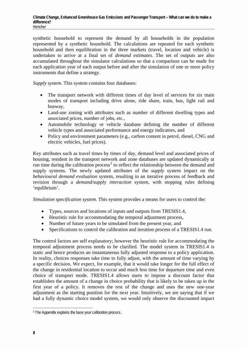
Climate Change, Enhanced Greenhouse Gas Emissions and Passenger Transport – What can we do to make a difference? Hensher synthetic household to represent the demand by all households in the population represented by a synthetic household. The calculations are repeated for each synthetic household and then equilibration in the three markets (travel, location and vehicle) is undertaken to arrive at a final set of demand estimates. The set of outputs are also accumulated throughout the simulator calculations so that a comparison can be made for each application year of each output before and after the simulation of one or more policy instruments that define a strategy. Supply system. This system contains four databases:

• The transport network with different times of day level of services for six main modes of transport including drive alone, ride share, train, bus, light rail and busway,

• Land-use zoning with attributes such as number of different dwelling types and associated prices, number of jobs, etc.,

• Automobile technology or vehicle database defining the number of different vehicle types and associated performance and energy indicators, and

• Policy and environment parameters (e.g., carbon content in petrol, diesel, CNG and electric vehicles, fuel prices).

Key attributes such as travel times by times of day, demand level and associated prices of housing, resident in the transport network and zone databases are updated dynamically at run time during the calibration process3 to reflect the relationship between the demand and supply systems. The newly updated attributes of the supply system impact on the behavioural demand evaluation system, resulting in an iterative process of feedback and revision through a demand/supply interaction system, with stopping rules defining ‘equlibrium’. Simulation specification system. This system provides a means for users to control the:

• Types, sources and locations of inputs and outputs from TRESIS1.4, • Heuristic rule for accommodating the temporal adjustment process, • Number of future years to be simulated from the present year, and • Specifications to control the calibration and iteration process of a TRESIS1.4 run.

The control factors are self explanatory; however the heuristic rule for accommodating the temporal adjustment process needs to be clarified. The model system in TRESIS1.4 is static and hence produces an instantaneous fully adjusted response to a policy application. In reality, choices responses take time to fully adjust, with the amount of time varying by a specific decision. We expect, for example, that it would take longer for the full effect of the change in residential location to occur and much less time for departure time and even choice of transport mode. TRESIS1.4 allows users to impose a discount factor that establishes the amount of a change in choice probability that is likely to be taken up in the first year of a policy. It removes the rest of the change and uses the new one-year adjustment as the starting position for the next year. Intuitively, we are saying that if we had a fully dynamic choice model system, we would only observe the discounted impact

3 The Appendix explains the base year calibration process.

8


Hensher

after each year. Different discount factors can be specified to control the temporal process of change for different choice models in TRESIS1.4. Policy specification system. There is richness in the array of policy instruments supported in TRESIS1.4 (Table 2) such as new public transport, new toll roads, congestion pricing, gas guzzler taxes, changing residential densities, introducing designated bus lanes, implementing fare changes, altering parking policy, introducing more flexible work practices, and the introduction of more fuel efficient vehicles4.

Table 2: Classification of Policy Instruments via Key Input Data in TRESIS1.4

Specific Policy Attributes Specific Location

Application

Times of Day (TOD)

Categories

New/Existing Public Transport

Frequency; Travel Time; Fare; Access; Egress

Origin-Destination

6 Spatial, Economic

New/Existing Roadway Distance; Capacity; Auto Travel Time; Congestion Pricing; Variable User Charges; Toll Cost

Origin-Destination

6 Spatial, Economic

Parking Charges Dollars/hour Destination 6 Spatial, Economic Urban Density 3 categories: Houses; Semi-

detached; Apartment/Flat and Associated Prices

Origin Non Spatial, Economic

Carbon Tax Carbon Tax (cents/kg) Not Location Specific

Non Economic

GST on New Vehicles On New Vehicle (from 2000) Not Location Specific

Non Economic

Automobile Technology Mass (kg); Whole Sale Price ($); Acceleration (secs to 100 km/h); Fuel Efficiency: City (L/100 km); Highway (L/100 km)

Not Location Specific

Non Economic, Energy, Environment

Fuel Excise by Fuel Type Wholesale Price of Petrol (cents/litre); Excise Component of Price of Petrol (cents/litre); Wholesale Price of Diesel (cents/litre); Excise Component of Price of Diesel (cents/litre)



Maximum Ages of Vehicles for Scrapping High Emitters

Maximum Vintage to Remove the High Emitters from Specific Classes of Vehicles (e.g. 16 years)



Vehicle Registration Charges

Dollars/Year for Different Vehicle Classes and Types


Non Economic, Energy

Fuel Efficiency of Current Fleet

Percentage of Fuel Efficiency of Current Fleet


Non Energy

Alternative Fuels-CNG Vehicles

6 Classes (from class 11 to class 16)



Price Rebate/Discounts on Vehicles

Rebate on New Vehicles Not Location Specific


4 The policy specification system employs a graphical and map-based (Map Objects) user interface to translate a single or mixture of policy instruments into changes in the supply systems.

9

Climate Change, Enhanced Greenhouse Gas Emissions and Passenger Transport – What can we do to make a difference? Hensher Behavioural demand evaluation system. Given the inputs from the behavioural demand specification system and the supply system, the characteristics of each synthetic household are used to derive the full set of behavioural choice probabilities for the set of travel, location and vehicle choices and predictions of vehicle use. Demand/Supply interaction system. This system contains three key procedures to control or equilibrate the three different types of interactions between demand and supply. The key mechanism for driving these three procedures is the level of interactions between demand and supply. Details of the underlying procedures is given in Hensher (2002). The three procedures are briefly described as follows (see Figure 4):

• Equilibration in the residential location and dwelling type market. Total demand for different dwelling types in each residential location is calculated at any point in time. Excess demand will result in an increase in location rents and dwelling prices. In TRESIS1.4, dwelling prices for different dwelling types are used to clear the markets for dwelling types and locations, in the absence of data on location rents. Some allowance for unused stock in built in, creating a disequilibrium state.

• Equilibration in the automobile market. A vehicle price relative model is used to determine the demand for new vehicles each year. This model controls the relativities of vehicle prices by vintage via given exogenous new vehicle prices. A vehicle scrappage model is used to identify the loss of used vehicles consequent on vintage and used vehicle prices, where the latter are fixed by new vehicle prices in a given year. The supply of new vehicles is determined as the difference between the total household demand for vehicles and the supply of used vehicles after application of a scrappage model based on used vehicle prices.

• Equilibration in the travel market. Households might adjust their route choices between origin and destination, or trip timing and/or mode choice in response to changes in the transport system, particularly the travel time and cost values between different origins and destinations. In other words, different households can have different choices in responding to changes in different levels of service at different times of day.

Reporting system: This system performs a number of calculations to report the outcome of the interaction between supply and demand at different times of day and a total average annual figure. TRESIS1.4 delivers a comprehensive suite of outputs (Table 3) such as impacts on greenhouse gas emissions, accessibility, equity, air quality and household consumer surplus. The output is in the format of summary tables cross-tabulated by household types, household incomes and residential zones and in more detailed format by origin and destination (OD), by different times of day and by different simulation years.

10


Hensher

Input Specification (who, what policy and how at when and where)

No

Vehicle Scrapping Model

Behavioural Models

All Demand Matrices

Vehicle Equilibration Model

Travel Equilibration Model

Housing Equilibration Model

- Demand status (responses from every households)

- Supply status (responses from Land-use Transpoand Environment)

Calibrate All Models

Output Reporting Calculate All Results

(who would be affected by what policy by how at when and where)

Yes

Calibrated ?

Is base year?

Yes

Yes

No

Figure 4: TRESIS1.4 Simulation Process

11


Table 3: Classification of Key Output Data in TRESIS

Key Output (1) (2) (3) (4) (5) Categories Dwelling Demand by Types and Prices NA NA NA NA Yes Social, Spatial, Economic Vehicle Demand by Vehicle Classes/Vintages NA NA NA NA Yes Spatial, Economic Consumer Surplus NA NA NA NA Yes Spatial, Economic Accessibility NA NA NA NA Yes Spatial, Economic Estimated Travel Time/Traffic Volumes by OD Yes Yes Yes Yes Yes Spatial Total Trips by OD and Modal Shares NA Yes Yes Yes Yes Spatial Commuting Trips by OD NA Yes Yes Yes Yes Spatial Vehicle Kilometres (VKM) NA NA NA NA Yes Spatial, Environment Energy Consumed by 4 Different Types of Vehicles (petrol, diesel, CNG, electric)

NA NA NA NA Yes Energy, Environment

CO2 Produced by 4 Different Types of Vehicles (petrol, diesel, CNG, electric)

NA NA NA NA Yes Energy, Environment

End User Vehicle Cost (operating cost, registration and vehicle annualised cost)

Yes Yes Yes Yes Yes Social, Economic, Energy

End User Cost (both private and public transport cost)

Yes Yes Yes Yes Yes Social, Economic

End User Time (both private and public transport cost)

Yes Yes Yes Yes Yes Social, Economic, Energy

Government Revenue: Parking Charge Yes Yes Yes Yes Yes Spatial, Economic Government Revenue: Road Toll Yes Yes Yes Yes Yes Spatial, Economic Government Revenue: Congestion Charge /Variable user charge

Yes Yes Yes Yes Yes Spatial, Economic

Government Revenue: Vehicle Sale Tax Yes Yes Yes Yes Yes Economic Government Revenue: Fuel Excise Yes Yes Yes Yes Yes Economic, Energy,

Environment Government Revenue: Carbon Tax Yes Yes Yes Yes Yes Economic, Energy,

Environment Government Expenditure: Purchase of Old Vehicles

Yes Yes Yes Yes Yes Economic, Energy, Environment

Government Expenditure: Rebate for New Vehicle

Yes Yes Yes Yes Yes Economic, Energy, Environment

Note 1: (1) By household socio-economic characteristics, (2) By zone, (3) By transport modes, (4) By times of day, (5) By year of simulation Note 2: NA indicates ‘not available.’

3. Applications We have selected a number of policy instruments to investigate the policy-value of an integrated model system, and evaluated each in the context of the Sydney Statistical Division which includes the Sydney Metropolitan area and the Central Coast (Figure 5). Although TRESIS1.4 can evaluate a very large number of instruments (including mixtures of instruments and varying levels of treatment of each instrument), we have focused on three scenarios that show very real promise in reducing CO2 and three scenarios that have little impact, despite being promoted by some sections of society. To place GGE reductions in perspective, we report a range of very relevant performance measures to remind readers that the triple-bottom line approach to policy formulation and implementation must recognize the balance between efficiency, equity and sustainability, and encourage a review of options that results in action that contributes to the achievement of the objectives promoted by the range of stakeholders. One challenge is to identify

12


Hensher

which set of policy instruments can contribute in a non-marginal way to reducing CO2 while enhancing the broader set of efficiency and distributive justice objectives, including the budgetary implications for government. We focus on the impacts over the period from 2010 up to 2015. The year of introduction (i.e. the exogenous shock) starts in January, evaluating a policy annually, summing the impacts over time and reporting the findings for each year. The cost items are calculated in constant dollars (A$1998). We report aggregate outputs (at a city level) herein, although a number of disaggregate output options are available by zone, zone pair, household type, income group etc. (see Table 3). The selection of output indicators of interest is generally determined by the objectives of the study. For example, in an environmental evaluation, greenhouse gas emissions (i.e., CO2) is an appropriate indicator. In a strict economic analysis, vehicle operating cost and government revenue impacts also provide useful indicators. From a transport planning perspective, we may be interested in indicators such as modal share, total vehicle kilometres and trips between each origin-destination pair.

Figure 5 Sydney Case Study

Outer Western Sydney

Outer South Western Sydney

Gosford-Wyong

Blacktown-Baulkham HillsHornsby-Ku-ring-gai

Fairfield-Liverpool

St George-Sutherland

Northern Beaches

Central Wes tern Sydney

Inner SydneyInner Western Sydney

3

9

6

13

117

1

12

14

2

8

We have selected a range of indicators that enable us to consider the impact of each policy on efficiency, equity and sustainability. They are summarized in Table 4.

13


Table 4: List of Selected TRESIS1.4 Output

Performance Indicators

Description Units Note

TCO2 Total annual carbon dioxide Kilograms (kg)

Car (includes all passenger automobiles – sedan, wagons, utilities, panel vans, 4WD), based on 2.35kg CO2 per litre of petrol. The calculation of this output totally independent of the Carbon tax function. The carbon tax calculates total carbon content which is equal to carbon content rate x fuel consumed (litres). Carbon content rate is set at 0.635775 kg Carbon per litre of petrol

TEUC.MC Total annual end-use money cost Dollars ($98) All person trips, includes for car: op cost, car registration charges, annualised vehicle cost, parking, toll, congestion charge; and public transport fares

TEUC.TTC Total annual end-use travel time cost Dollars ($98) All person trips; with travel time for ride-share for each person in car (converted to $’s). This item also includes all components of time of public transport users

TEMUDTMC Total annual expected maximum utility from each model system for each of the model components defined - by departure time and mode choice (DTMC) links

Dollars ($98) Calculation uses full set of 36 (=6modesx6TODs) exp*V functions

TEMURLC Total annual expected maximum utility from each model system for each of the model components defined - by the linkage: residential location choice (RLC) links

Dollars ($98)

TVKM(km) Total annual passenger vehicle kilometers

Kilometres (km)

Car

VehOpCost Total annual auto VKM operating cost Dollars ($98) Car. Fuel prices assumed to increase by 0.05% paTGovtVehReg Total government revenue from auto

ownership Dollars ($98) Car

TGovtExcise Total government revenue from fuel excise

Dollars ($98) Car (petrol and diesel)

TGovtCarbT Total government revenue from carbon tax


TGovtSalesT Total government revenue from sales tax (GST post 2000)


TPark Total revenue from parking strategy Dollars ($98) Car TRCong Total revenue from congestion pricing Dollars ($98) Car TRVuC Total revenue for variable user charge Dollars ($98) Car TPT Total revenue from public transport use Dollars ($98) All PT (all modes, private and public). Fares

assumed to remain at $98 levels over 1999-2025 TDA Modal growth for car drive alone % All person trips TRS Modal growth for ride share % All person trips Ttrain Modal growth for train travel % All person trips Tbus Modal growth for bus travel % All person trips TLrl Modal growth for light rail travel % All person trips Tbwy Modal growth for busway use % All person trips

Note: A trip = a Person Trip (e.g., 2 person’s ride sharing = 2 person trips)

14


Hensher

The Vehicle operating cost variable needs special definition given its constituent parts. It comprises: VehOpCost = [{cityFuel*propCityF + hwyFuel*(1-propCityF)}*0.01] *

[tPricePetrol*(1-propnDiesel) + tPriceDiesel*propnDiesel + carbonTax * {carbLitD*propnDiesel+ carbLitP*(1-propnDiesel)}] + (cTank + carbonTax*carbTAlt) / rangealf + (cCharge + carbonTax* carbTElc) / rangeelc

where: cityFuel = city cycle fuel efficiency (litres/100 km) hwyFuel = highway cycle fuel efficiency (litres/100 km) propCityF = proportion of use which is in the city fuel cycle (default = 0.7) propnDiesel = proportion of conventional-fuelled vehicles using diesel tPricePetrol = wpricepetrol + expricepetrol (cents per litre) wpricepetrol = wholesale price of petrol (cents per litre) expricepetrol = excise component of price of petrol (cents per litre) tpricediesel = wpricediesel + expricediesel (cents per litre) wpricediesel = wholesale price of diesel (cents per litre) expricediesel = excise component of price of diesel (cents per litre) carbonTax = carbon tax (cents per kg) carbLitD = carbon per litre of diesel (kg/litre) carbLitP = carbon per litre of petrol (kg/litre) carbTElc = carbon per full electric recharge (kg) carbTAlt = carbon per tank of alternative fuel (kg) cTank = wctank + extank (cents) wctank = wholesale cost of a tank of alternative fuel (cents) extank = excise component of cost of a tank of alternative fuel (cents) cCharge = wccharge + excharge (cents) wccharge = wholesale cost of a full electric recharge (cents) excharge = excise component of cost of a full electric recharge (cents) rangeelc = range of electric vehicle on a fully charged battery (km) rangealf = range of alternative fuelled vehicle on a full tank (km)

The VehOpCost indicator excludes spatial cost strategies such as toll and congestion charge. It is strictly related to fuel-based strategies (changes in fuel efficiency, carbon tax, fuel excise). All elements are defined in TEUC.MC (Table 4).

TRESIS1.4 provides the results of these selected indicators for the base case and policy case for each application year, defined as:

• Base Case: This is a scenario of “business as usual” in each year. • Policy Case: A policy is implemented and its impact is evaluated by comparing the

output indicators between the base case and policy case (in both absolute and percentage terms).

Although outputs are obtained year by year, we focus on selected indicators in 2015 (Tables 5 and 6) that were first introduced in 2010. Table 5 provides details of the base and scenario absolute impacts and the difference for one specific policy, as a way of

15

Climate Change, Enhanced Greenhouse Gas Emissions and Passenger Transport – What can we do to make a difference? Hensher ensuring clarity in interpretation of the outputs. Table 6 focuses on the difference between the base and scenario for six scenarios. If a carbon tax of 20 cents/kg (referred to as Carbon20) were implemented (Table 5), the average vehicle operating cost after equilibration would increase by 16.61 percent. Total government revenue would increase by 9.34 percent. The total end-user money cost would increase by 4.57 percent while total end-user time cost would be reduced by 1.095 percent. Modal commuter growth for automobile trips would decrease while for public transport it would increase, especially for bus. Total annual vehicle kilometres would reduce by 2.53 percent and total CO2 would reduce by 2.671 percent. The overall expected maximum utility (or consumer surplus) reduction summed across the entire model system is 3.254 percent. When the expected maximum utility for mode and departure time choice is conditioned on location, there is a positive 2.054 percent gain in consumer surplus. This indicates that subsequent adjustments in workplace and or residential location has resulted in a loss of surplus that in the short run was gained through modal and departure time trip adjustments. One can obtain these indicators for each application year in the evaluation period, and calculate the accumulated impact of the policy over a given period.

Table 5: Summary results for 20c/kg carbon tax: 2015

(Policy enacted from 2010) Indicators Base case Carbon tax 20c/kg Difference (%) Automobile operating cost AvOpCost (c/km) 7.175E+00 8.367E+00 16.61% VehOpCost ($) 2.33E+09 2.648E+09 13.66% Government revenue TGovtCarbT ($) 0 3.884E+08 N/A TGovtExcise ($) 1.469E+09 1.43E+09 -2.674% TGovtPark ($) 8.475E+08 8.447E+08 -0.334% TgovtPT ($) 9.508E+08 1.065E+09 12.03% TGovtSales ($) 3.555E+08 3.573E+08 0.489% TGovtVehReg ($) 8.729E+07 8.714E+07 -0.168% Subtotal 3.71E+09 4.17E+09 9.34% Total end user cost TEUC.MoneyC ($) 8.866E+09 9.271E+09 4.565% TEUC.TimeC ($) 3.153E+10 3.119E+10 -1.095% Consumer surplus: Entire model system (TEMURLC) ($) 7.621E+10 7.619E+10

-3.254%

Mode and departure time (TEMUDTMC) ($) -6.661E+14 -6.798E+14

2.054%

Commuter Mode growth TDA 2.034E+09 2.01E+09 -1.441% TRS 9.624E+08 9.508E+08 -1.296% TTain 2.054E+08 2.273E+08 1.067% TBus 1.765E+08 1.901E+08 7.687% Greenhouse gas emissions TCO2 (kg) 8.59E+09 8.36E+09 -2.671% Passenger vehicle kilometres TVKM (km) 3.189E+10 3.108E+10 -2.530%

16

Climate Change, Enhanced Greenhouse Gas Emissions and Passenger Transport – What can we do to make difference?

Hensher

17

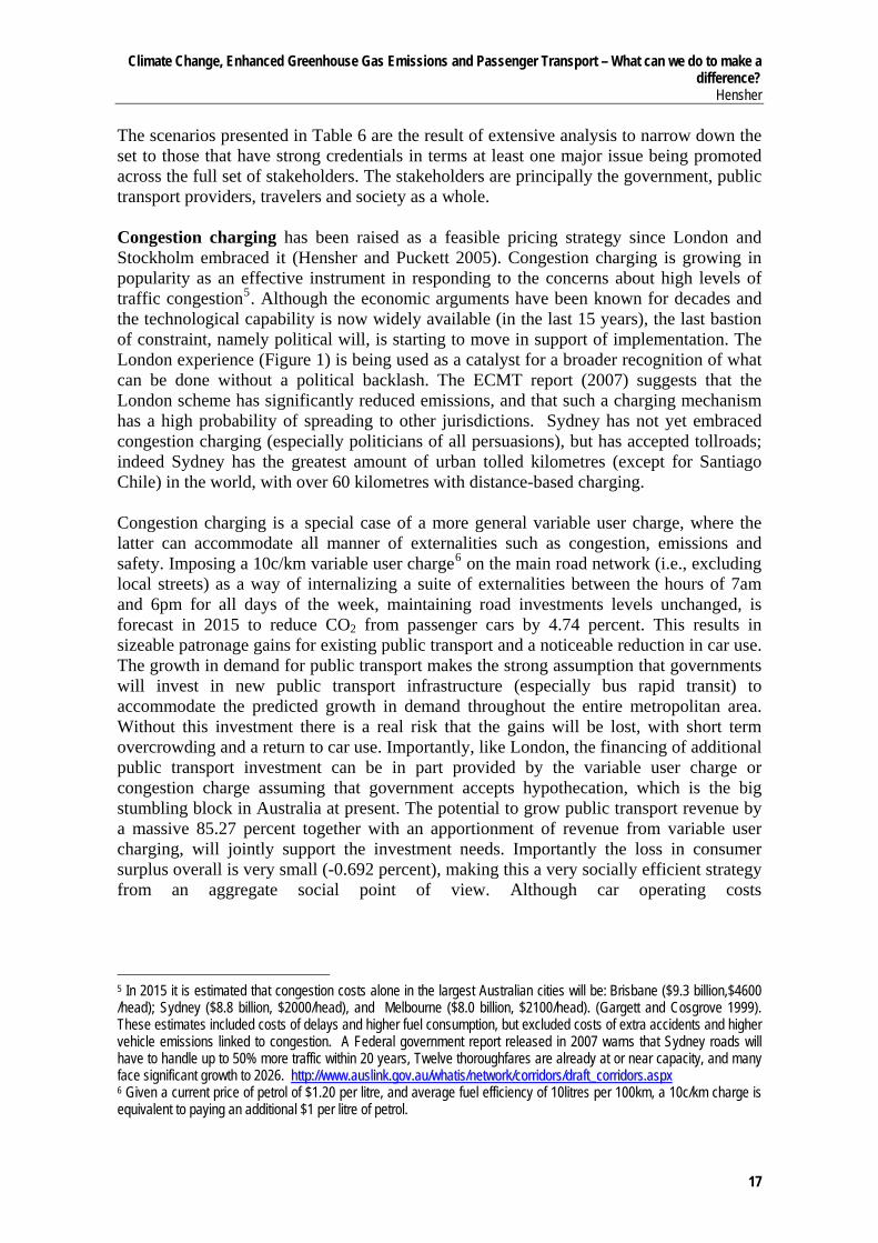
The scenarios presented in Table 6 are the result of extensive analysis to narrow down the set to those that have strong credentials in terms at least one major issue being promoted across the full set of stakeholders. The stakeholders are principally the government, public transport providers, travelers and society as a whole. Congestion charging has been raised as a feasible pricing strategy since London and Stockholm embraced it (Hensher and Puckett 2005). Congestion charging is growing in popularity as an effective instrument in responding to the concerns about high levels of traffic congestion5. Although the economic arguments have been known for decades and the technological capability is now widely available (in the last 15 years), the last bastion of constraint, namely political will, is starting to move in support of implementation. The London experience (Figure 1) is being used as a catalyst for a broader recognition of what can be done without a political backlash. The ECMT report (2007) suggests that the London scheme has significantly reduced emissions, and that such a charging mechanism has a high probability of spreading to other jurisdictions. Sydney has not yet embraced congestion charging (especially politicians of all persuasions), but has accepted tollroads; indeed Sydney has the greatest amount of urban tolled kilometres (except for Santiago Chile) in the world, with over 60 kilometres with distance-based charging. Congestion charging is a special case of a more general variable user charge, where the latter can accommodate all manner of externalities such as congestion, emissions and safety. Imposing a 10c/km variable user charge6 on the main road network (i.e., excluding local streets) as a way of internalizing a suite of externalities between the hours of 7am and 6pm for all days of the week, maintaining road investments levels unchanged, is forecast in 2015 to reduce CO2 from passenger cars by 4.74 percent. This results in sizeable patronage gains for existing public transport and a noticeable reduction in car use. The growth in demand for public transport makes the strong assumption that governments will invest in new public transport infrastructure (especially bus rapid transit) to accommodate the predicted growth in demand throughout the entire metropolitan area. Without this investment there is a real risk that the gains will be lost, with short term overcrowding and a return to car use. Importantly, like London, the financing of additional public transport investment can be in part provided by the variable user charge or congestion charge assuming that government accepts hypothecation, which is the big stumbling block in Australia at present. The potential to grow public transport revenue by a massive 85.27 percent together with an apportionment of revenue from variable user charging, will jointly support the investment needs. Importantly the loss in consumer surplus overall is very small (-0.692 percent), making this a very socially efficient strategy from an aggregate social point of view. Although car operating costs

5 In 2015 it is estimated that congestion costs alone in the largest Australian cities will be: Brisbane ($9.3 billion,$4600 /head); Sydney ($8.8 billion, $2000/head), and Melbourne ($8.0 billion, $2100/head). (Gargett and Cosgrove 1999). These estimates included costs of delays and higher fuel consumption, but excluded costs of extra accidents and higher vehicle emissions linked to congestion. A Federal government report released in 2007 warns that Sydney roads will have to handle up to 50% more traffic within 20 years, Twelve thoroughfares are already at or near capacity, and many face significant growth to 2026. http://www.auslink.gov.au/whatis/network/corridors/draft_corridors.aspxhttp://www.auslink.gov.au/whatis/network/corridors/draft_corridors.aspx 6 Given a current price of petrol of $1.20 per litre, and average fuel efficiency of 10litres per 100km, a 10c/km charge is equivalent to paying an additional $1 per litre of petrol.

a

http://www.auslink.gov.au/whatis/network/corridors/draft_corridors.aspx


































































nge, Enhanced Greenhouse Gas Emissions and Passenger Transport – What can we do to make a difference?

Table 6: Summary results for Various Policy Instruments 2015 (Policy enacted from 2010)

Indicators 10c/km

variable user charge –

metro area 7am – 6pm

25c/km congestion charge in CBD only

7am – 6pm

$16 cordon charge CBD only 7am-

6pm

Double bus frequency (i.e. half

headway)

10c/km Congestion

charge – metro area 7am-6pm;

double bus frequency

Rail and bus fares

reduced by 50%

Fuel efficiency improvement

by 25%

Carbon tax 40c/kg

Auto operating cost VehOpCost -4.73% -0.1261% -0.040% -0.167% -4.624% -0.441% 21.26% 26.95% Government revenue ($) TGovtCarbT ($) - - - - - - - 7.585E+08 TCong, TVuC ($) 2.947E+09 8.418E+07 2.68E+06 - 3.129E+09 - - - TGovtExcise -4.755% -0.126% -0.4036% -0.161% -4.65% -0.425% -21.26% -4.959% TGovtPark -5.12% -13.08% -29.08% -1.84% 7.26% -7.96% 0.2989% 0.673% TgovtPT 85.27% 1.186% 4.048% 58.5% 44.67% 16.1% -12.28% 25.67% TGovtSales 0.436% -0.0012% -0.0036% -0.11% -.0347% -0.322% 0.588% 0.971% TGovtVehReg 3.471% -0.0011% -0.0027 -0.09% -.0272% -0.271% 0.1832% 0.342% Subtotal 79.3% -12.02% -25.71% 56.3% 47.44% 7.12% -32.47% 22.7% Total end user cost TEUC.MoneyC 29.65% -0.754% -0.5033% 5.97% 25.7% -3.86% 6.632% 9.172% TEUC.TimeC 9.24% 0.190% 0.4045% -5.35% 5.455% -3.17% 1.177% -2.298% Consumer surplus: Entire model system TEMURLC -0.692% -0.0007% -0.0017% 0.0359% -0.4469% 0.0538% 0.0753% -0.0072% Mode and departure time (TEMUDTMC) 10.53%

-0.098%

-0.165%

-9.259% 18.91%

-13.34%

-2.963%

4.067%

Commuter Mode growth* TDA -10.58% -0.369% -0.8385% -6.951% -5.527% -7.469% 1.521% -3.027% TRS 11.65% -0.083% -0.1964% -8.444% -5.596% -6.232% 1.40% -2.716% TTrain 73.3% 1.329% 3.091% -2.725% 78.87% 49.71% -11.18% 22.48% TBus 74.0% 2.509% 5.772% 121.1% -19.02% 45.43% -8.293% 16.01% TLight Rail 11.5% 16.59% 38.56% -6.24% 17.57% -10.24% -3.854% 7.537% TBwy 154.8% 0.8199% 1.901% 5.153% 151.9% -9.738% -16.78% 3.83% Greenhouse gas emissions TCO2 (kg) -4.75% -0.126% -0.4036% -0.1609% -4.634% -0.423% -21.26% -4.952% Passenger vehicle kms TVKM (km) -4.686% -0.125% -0.3998% -0.0151% -4.583% -0.397% 4.803% -4.679%

• These percentages are growth in patronage, noting that bus and train is off a very small base of approximately 6% and 4% respectively. • Run times vary from 30 minutes to 1 hour.

Climate ChaHensher


Hensher

will decrease by 4.73 percent on average, when the adjustment in monies outlaid on variable user charges, tolls and public transport fares is added in, the total end user monetary cost increases by 29.65 percent. Added to this will be the increase in total end user travel time cost of 9.24 percent, due in aggregate to increased travel times by public transport despite improved travel times for car users. In contrast to a metropolitan-wide variable user charging scheme, if we were to limit the charge to the Central Business District (CBD) of Sydney, as a congestion charge that has been mooted many times in the Sydney media, and charged at 25 cents/km7, the impact on CO2 is very small indeed, namely 0.126 percent. Likewise the impact on consumer surplus and car use is small, although the switching that occurs benefits light rail in particular (which currently only serves the southern end of the CBD) and results in sizeable revenue reductions for the parking stations in the CDB (-13.08 percent overall). Such a location-specific charging scheme is not recommended since it delivers very small social benefits. It is however relatively easier to implement than a metropolitan-wide scheme in the sense of requiring major investment in public transport, and may have value in demonstrating the merits of a congestion charging scheme that might be rolled out across the entire system in due course. If we were to impose a London-styled charge on the CBD of Sydney, this is equivalent to approximately $16 per day. This raises $84m per annum but does relatively little to reduce CO2 emissions, primarily because of the dominance of travel which does not go to or from the CBD by car. In the peak in Sydney, for example, nearly 80 percent of all trips to the CBD are by public transport. The cars that travel into the CBD are predominantly company cars with permanent parking who are somewhat price insensitive. The substantial reduction in car parking revenue is from casual parkers, not permanents. One of the challenges is to ensure that the revenue raised is in part allocated back to the transport sector to improve public transport (adding to the 4.05 percent increase in public transport revenue from switchers). Table 7 summarises the costs and benefits associated with the Stockholm congestion charging cordon. Eliasson (2007) undertook an initial cost-benefit analysis and found that the system is shown to yield a significant social surplus, well enough to cover both investment and operational costs, provided that it is kept for a reasonable lifetime. Investment costs are recovered (in terms of social benefit) in about four years. An alternative with similar policy outputs to a variable user or congestion charge is a carbon tax imposed on the carbon-based energy sources according to their carbon contents. Carbon taxes are implemented to reduce CO2 emissions emitted into the atmosphere, through their pricing effects on fuel consumptions and energy selection (Zhang and Baranzini 2004). Sweden is the first country that introduced the carbon tax in 1991 with US$30 per tonne of emitted CO2, increasing to US$46 per tonne of emitted CO2 after 1997 (Brännlund and Nordström 2004). Finland, the Netherlands, and Norway also introduced carbon taxes in the 1990s. New Zealand proposed a carbon tax at NZ$15 per tonne of emitted CO2 (Wikipedia 2007). So far, the Australian Government has not developed a carbon tax as part of its greenhouse policies, although there is active dialogue. The carbon content in TRESIS1.4 is set at 0.635775 kg Carbon per litre of petrol. If a carbon tax of 5c per kg is considered for petrol

7 This is a massive $2.50 per litre of fuel equivalent; however the amount of kilometres is relatively small. It is noteworthy than some Sydney travellers pay $3-$4 in tolls for trips as short as 10 kilometres.

19

http://en.wikipedia.org/wiki/Finland

http://en.wikipedia.org/wiki/The_Netherlands

http://en.wikipedia.org/wiki/Norway

Climate Change, Enhanced Greenhouse Gas Emissions and Passenger Transport – What can we do to make a difference? Hensher this would be 3.18 cents per litre, and for diesel it is 3.67 cents per litre. These cost impacts are reflected in modelled vehicle use.

Table 7: The Stockholm Charging Scheme: A CBA Assessment8

million SEK per year Loss/gain Shorter travel times 496 More reliable travel times 78 Loss for evicted car drivers, gain for new car drivers -68 Paid congestion charges -763 Consumer surplus, total -257 Less greenhouse gas emissions 64 Health and environmental effects 22 Increased traffic safety 125 Other effects, total 211 Paid congestion charges 763 Operational costs for charging system (incl. reinvestment and maintenance) -220 Increased public transit revenues 184 Necessary increase in public transport capacity -64 Decreased revenues from fuel taxes -53 Decreased road maintenance costs 1 Public costs and revenues, total 611 Marginal cost of public funds, shadow price of public funds 118 Total socioeconomic surplus, excl. investment costs 683

A 40c/kg carbon charge9 delivers a very similar reduction in CO2 as a metro-wide congestion charge of 10c/km; however while it increases car operating costs by 26.95 percent, it increases overall total end use money costs by 9.17 percent, considerably less that the 29.6 percent for a 10c/km variable user charge. Interestingly the reduction in total car kilometres is very similar (4.679 and 4.686 percent respectively for 40c/kg carbon tax and 10c/km variable user charge). The overall loss in consumer surplus is very small (.0-0.0072 percent) but the gain associated with mode and departure time choice switching is much smaller (4.067 percent) than the 10.5 percent associated with the congestion charge. Likewise the switch to public transport, while impressive, is considerably lower than for a congestion charge; and may well be more sustainable and deliverable in terms of requisite increases in public transport investment. The most important implication of this comparative assessment is that a carbon tax (at the appropriate rate) can deliver many of the major benefits for a smaller investment in public transport and lower impost on all travellers than a congestion charge (at the evaluated costs) for the equivalent reduction in CO2. 8 Table 7 shows that the congestion charges produce a net social benefit of a little less than 700 mSEK/year (around 80 mEuro/year). Consumer surplus is negative, as expected, but the value of the time savings gains is high compared to the paid charges – time gains amount to around 70% of the paid charges, which is very high compared to most theoretical or model-based studies. This is mainly due to “network effects”, i.e. significant amounts of traffic that do not cross the cordon and hence do not pay any charge but still gain from the congestion reduction. “Other” effects – environmental effects and improved traffic safety – is valued to 211 mSEK/year. The total public financial surplus is 611 mSEK/year, of which 542 mSEK is net revenues from the charges and 184 mSEK is increased revenues from public transport fares. The yearly cost of the system (220 mSEK) includes necessary reinvestments and maintenance such as replacement of cameras and other hardware, and also certain additional costs such as moving charging portals when the building of a northern bypass starts in the summer of 2007. 9 A 40c/kg carbon tax on petrol is equivalent to an additional 25.44 cents per litre on fuel, which is currently $1.20 per litre.

20


Hensher

An at source instrument is improved vehicle fuel efficiency (in litres per 100km). We have assumed a capability of improving fuel efficiency by 25 percent. This is directly linked into CO2 with a 21.26 percent reduction by 2015 after accounting for the stimulus to increased vehicle kilometers (4.803 percent increase), in part due to a switch from public transport but also linked to reduced cost of motoring per kilometer. The switch from public transport combined with additional travel increases total end use monetary costs for all trip activity by 6.632 percent and small increase in end use travel time cost of 1.17 percent. Surprisingly this rebalancing of travel activity has a very small positive influence on overall net consumer surplus (0.0753 percent), although a more noticeable loss of net surplus (-2.963 percent) as a result of modal and departure time switching holding residential and workplace location fixed. Government is a financial looser to the tune of -32.47 percent. There are many pundits that still believe that we can harness sustainability gains by focusing strictly on improvements in public transport. This is highly unlikely as mounting evidence suggests10, but politically it seems to have greater appeal, in large measure because one is not flirting with prices except to decrease or freeze them to a consumer price index adjustment. In recognition that ‘frequency, connectivity and visibility’ are key elements of a strategy to grow public transport patronage, we investigated improved frequency, doubling it (i.e., halving headways) throughout the entire metropolitan bus network, public sand private. We did not change the train services given the difficulty in achieving such changes.11 We also looked at reducing rail and bus fares, since this is a regular recommendation by some stakeholders. Doubling bus frequencies does very little to reduce CO2, but given that buses share roads with cars, it adds to the overall money cost of road use (attributable to increased payment of public transport fares) but a significant improvement in time costs (due to modal substitution) of -5.35 percent. Clearly this is a potential winner for bus operators (58.5 percent growth in fare revenue); however this has to be contrasted with the cost of extra vehicles and other inputs (labour, fuel, maintenance etc). Reducing bus and train fares by 50 percent does attract patronage, but it does very little to reduce CO2 associated with car kilometres. This is generally well known. It does impact on parking station revenue (given that most of the added rail patronage is to and from CBD where parking is expensive). In our application we have not reduced fares on premium busway services such as those on tollroads and dedicated roads such as Liverpool-Parramatta Transitway, and light rail. The consumer surplus gains overall are very small (0.0538 percent) and indeed there is a reduction of 13.34 percent when focusing on mode and departure time, holding residential and workplace location fixed. What this suggests is that the increased demand adds crowding delays that more than offset any financial gains. Clearly the fare reduction would require substantial investment in service levels to be able to recapture these lost benefits. Finally we combined variable user charging with a doubling of bus frequency, and as might be expected the dominant gains are attributable to the 10c/km variable user charge. The

10 The EMCT (2007) review states that “Modal shift policies are usually weak in terms of the quantity of CO2 abated” (page 18). 11 The NSW Government, in 2006, reduced frequencies in the off peak in order to ensure greater on-time running, but increased frequency on some peak services.

21

Climate Change, Enhanced Greenhouse Gas Emissions and Passenger Transport – What can we do to make a difference? Hensher frequency effect does impact strongly on the gain in consumer surplus for mode and departure time switching, holding location constant.

Conclusions Although the passenger transport sector is a relatively small player in the overall production of CO2 emissions (8 percent of national emissions in Australia in 2006), with the stationary energy sector being the main contributor, the concerning rate of increase (1.5 percent per annum) and high visibility of automobility ensures itself a major place on the reform agendas of many nations working to reduce CO2 emissions and hence contributing to the resolution of the climate change challenge. The policy scenarios assessed herein highlight the most probable extent to which the passenger transport sector can contribute to reducing CO2 through pricing instruments directed explicitly to car use as well as initiatives directly related to public transport to make it more attractive. We believe that these types of instruments can only at best, reduce CO2 by five percent, with the carbon tax offering the most attractive way forward when balancing efficiency, equity and sustainability considerations. Indeed the ECMT (2007) progress reviews states that “Carbon and fuel taxes are the ideal measures for addressing CO2 emissions. They send clear signals and distort the economy less than any other approach.” (page 13). We have not considered the likely impact of alternative (non-fossil) fuels and greater investment in more fuel efficient petrol and diesel fired engine technology; which have promise to reduce the growth in CO2 beyond 5 percent. We ran an across the board 25 percent improvement in fuel efficiency in 2015 which suggests 21.25 percent reduction in CO2. This supports the position of the ECMT (2007) that fuel efficiency delivers most in terms of energy efficiency and is relatively cost effective. What it does do however is attract more cars and hence vehicle kilometres onto the road system, which increases traffic congestion. Overall it appears that a mix of technology (i.e., fuel efficiency improvements) and pricing through a carbon tax or a variable user charge is way forward assuming continuing use of fossil fuels. The carbon tax, in the presence of improved fuel efficiency is likely to be linked to reduced CO2 per vehicle kilometre and hence will not have as great an impact on reduced vehicle kilometres travelled as a variable user charge. On balance we favour the mix of improved fuel efficiency and a variable user charge which should move to meet targets being promoted in many countries. As an example, a 5 c/km variable user charge throughout the Sydney metropolitan area on all main roads, combined with an achieved 15 percent improvement in the fuel efficiency of the car stock, is forecast to deliver in 2015 a 15 percent reduction in CO2. This also produces a desirable financial outcome for government given that fuel efficiency improvement alone will shrink government coffers quite markedly. Finally, it is important to recognize that forecasts based on each policy instrument carry varying degrees of forecast uncertainty, in part linked to the specification of TRESIS1.4 but also markedly influenced by the ability of stakeholders to actually implement the specific policies at the levels assessed. We are of the belief that technological solutions (e.g., those linked to improved vehicle fuel efficiency) are somewhat more feasible to achieve than

22


Hensher

commitments of government to introduce a carbon tax, a variable user charge or a congestion charge, and hence should be given more feasibility weight, despite the revenue losses to government pursuant of a technological focus alone. The comparative advantage of technological change is that it is being invested in globally; whereas non-technological instruments (which may actually speed up the commercialization of technology instruments) are subject to the politics of a jurisdiction, no matter how much groundswell there is globally for specific actions.

References

ABS (2006) Survey of Motor Vehicle Use, Australia, 01 Nov 2004 to 31 Oct 2005, cat. no. 9208.0. Retrieved from AusStats database.

ABS (2007) Greenhouse Gas Emissions, Australian Bureau of Statistics, Canberra.

Australian Greenhouse Office (2006) Reducing greenhouse gas emissions. http://www.greenhouse.gov.au/fuelguide/environment.html

Australian Greenhouse Office (2006a), Transport Sector Greenhouse Gas Emissions Projections 2006, Australian Government, December.

Brännlund, R and Nordström, J. (2004) Carbon tax simulations using a household demand model, European Economic Review, Vol. 48, Iss. 1, pp. 211-233.

Bureau of Transport and Regional Economics (2005), Greenhouse Gas Emissions from Australian Transport: Base Case Projections to 2020, Report to the Australian Greenhouse Gas Office, Department of the Environment and Heritage, August.

ECMT (2007) Cutting Transport CO2 Emission: What Progress?, ECMT, Paris.

Eliasson, J. (2007) Cost-benefit analysis of the Stockholm congestion charging system Transek AB, Stockholm.

Evans, R. (2006) Nine lies about global warming, The Lavoisier Group, Sydney. February.

Gargett, David and Cosgrove, David, Urban Transport – Looking Ahead, Information Sheet 14, Canberra: Commonwealth of Australia, Bureau of Transport Economics, 1999.

Hensher, D.A. (2002) A systematic assessment of the environmental impacts of transport policy: an end use perspective, Environmental and Resource Economics. 22(1-2), pp 185-217

Hensher, D. A. (2003) Integrated Transport Models for Environmental Assessment. In D. A. Hensher, & K. Button (Eds.), Handbooks in Transport, Vol. 4. Oxford: Pergamon Press.

Hensher, D. A., and Greene, W. H. (2001) Choosing between conventional, electric and LPG/CNG vehicles in single-vehicle households. In D. A. Hensher (Ed.), Travel Behaviour Research: The Leading Edge: 725-749. Oxford: Pergamon Press.

Hensher, D. A., Milthorpe, F. W., and McCarthy, M. (1995) Greenhouse Gas Emission and the Demand for Urban Passenger Transport: Behavioural Model Estimation and Inputs into the ITS/BTCE Strategy Simulator: 1-103. Sydney: Institute of Transport Studies, The University of Sydney.

23

http://www.greenhouse.gov.au/fuelguide/environment.html

Climate Change, Enhanced Greenhouse Gas Emissions and Passenger Transport – What can we do to make a difference? Hensher Hensher, D. A., and Ton, T. (2002) TRESIS: A transportation, land use and environmental strategy impact simulator for urban areas. Transportation, 29: 439-457.

Hensher, D.A. and Puckett, S. (2005) Road user charging: the global relevance of recent developments in the United Kingdom, Transport Policy, 12, 377-83.

Hensher, D.A, Ton, T. and Kim, K.S (2005) Review of Tresis as a strategic advisory tool for evaluating land use and transport policies, Road and Transport Research, 14 (3), September, 34-49.

Stern Review (2006), The Economics of Climate Change. http: www.hm-treasury.gov.uk/media/8AC/F7/Executive Summary.pdf. Accessed 11/01/2007.

Ton, T., and Hensher, D. A. (2001) Synthesising Population Data: The Specification and Generation of Synthetic Households in TRESIS. Paper presented at the 9th World Conference on Transport Research, Seoul.

Warren, J. (ed.) (2007) Managing Transport Energy, Oxford University Press, Oxford.

Wikipedia (2007) Carbon tax. Retrieved from http://en.wikipedia.org/wiki/Carbon_tax

Zhang, Z. X. and Baranzini, A. (2004) What do we know about carbon taxes? An inquiry into their impacts on competitiveness and distribution of income, Energy Policy, Vol. 32, Iss. 4; pp. 507-518.

24

http://www.hm-treasury.gov.uk/media/8AC/F7/Executive%20Summary.pdf

http://www.hm-treasury.gov.uk/media/8AC/F7/Executive%20Summary.pdf


Hensher

Appendix A base year for model development and implementation has to be selected (in the case study, we use 1998, with December the actual time point at which to measure all activities and external data such as vehicle registrations and population). The system has to be calibrated for the base year population profiles and then applied annually with summaries of outputs for each year over the range of specified years. Each of the behavioral models has to be calibrated to reproduce the base year shares and total on each alternative. Once the models are calibrated, the parameter set remains unchanged in all applications. New calibration is required when base input data are changed. The data items selected for calibration in the case study are shown in Table A1.

Table A1: Base Year Calibration Criteria

Decision Block Data Criterion Location (per location) dwelling type share

total number of households total number of workers household fleet size distribution (0,1,2,3+)

Vehicle (per vehicle class) vehicle class shares total registered passenger vehicles total passenger vehicle kilometers household fleet size composition

Travel commuter mode share travel time (origin-destination) commuter departure time profile sample spatial and temporal work practice

composition

25

itls-wp-07-08 - the university of sydney business school

Documents