Iterative Learning Control for Accurate Task-Space Tracking withHumanoid Robots

Pranav A. Bhounsule1 and Katsu Yamane2

Abstract— Precise task-space tracking with manipulator-typesystems requires accurate kinematics models. In contrast totraditional manipulators, it is difficult to obtain an accuratekinematic model of humanoid robots due to complex structureand link flexibility. Also, prolonged use of the robot will leadto some parts wearing out or being replaced with a slightlydifferent alignment, thus throwing off the initial calibration.Therefore, there is a need to develop a control algorithm thatcan compensate for the modeling errors and quickly retuneitself, if needed, taking into account the controller bandwidthlimitations and high dimensionality of the system. In this paper,we develop an iterative learning control algorithm that canwork with existing inverse kinematics solver to refine the joint-level control commands to enable precise tracking in the taskspace. We demonstrate the efficacy of the algorithm on a theme-park type humanoid that learns to track the figure eight in 18trials and to serve a drink without spilling in 9 trials.

I. INTRODUCTION

Many applications of manipulator-type systems involveprecise task-space control. For example, industrial manipula-tors that do welding or personal humanoid robots that foldsclothes. Industrial manipulators rely on good CAD modelsand high-gain servo controllers to accomplish precise end-effector motions. However, the techniques that work well forindustrial manipulators may not transfer to humanoid robotsfor the following reasons:

1) Humanoid robots are made light weight due to weightand size constraints leading to flexible links. Thus,traditional CAD models which are based on rigid bodyassumptions are not valid. Additional modeling termsare needed to account for link flexibility, which can behard.

2) Humanoid robots tend to have small actuators forsafety reasons and/or may have a low bandwidthcontroller. This makes it hard to implement a preciseservo.

3) Humanoid robots have large number of joints. Thus,small parameters errors in the CAD model can lead tobig errors at the end-effectors.

4) When Humanoid robots are used long-term (e.g., per-sonal robots), some parts may wear out or be replacedwith a slightly different alignment. Hence the originalCAD model is not valid anymore.

Thus, for accurate task-space control of humanoid robots,one needs a method that can compensate for the modeling

1 Dept. of Mechanical Engineering, University of Texas SanAntonio, One UTSA Circle, San Antonio, TX 78249, USA.pranav.bhounsule@utsa.edu. 2 Disney Research, 4720Forbes Avenue, Lower Level, Suite 110 Pittsburgh, PA 15213, USA.kyamane@disneyresearch.com

errors by modifying the joint-level control commands andto make up for part wear and/or replacement. We presentan iterative learning control algorithm that can address theabove issues.

In this paper, we show that a combination of constrainedoptimization and iterative learning control can enable highfidelity position tracking. We use constrained optimization tosolve the inverse kinematics using the imperfect kinematicmodel. The cost for the constrained optimization is theweighted squared sum of the deviation of the end-effectorfrom the desired pose. The result of the constrained optimiza-tion is the joint motion as a function of time to produce thedesired end-effector motion. However, when the motion isimplemented on the robot, there is substantial tracking errorsbecause of the imperfect kinematic model. So next, we use it-erative learning control to improve the tracking performance.The iterative learning control algorithm modifies the desiredend-effector motion based on end-effector tracking errors toaccount for modeling errors. We try out two example motionson the humanoid: (i) drawing the figure eight, and (ii) servinga drink without spilling.

II. BACKGROUND AND RELATED WORK

The main issue with task-space control is the lack ofaccurate kinematic models due to reasons mentioned earlier.Traditional feedback control methods such as Proportional-Integral-Derivative Control [1] are the preferred methodsto correct for modeling errors because they have a simplestructure and can be relatively easy to hand-tune. However,they are not preferred when the plant is subject to unexpecteddisturbances. In this case, it is common to have an adaptivecontroller that modifies the control parameters to make up forthe varying loads [2], [3]. However, most feedback controltechniques rely on setting high gains which necessitates theuse of high bandwidth feedback control, typically 500 Hz ormore. In our case, the control bandwidth of 120 Hz limitsus to relatively low gains.

Learning based method have also been used to do task-space control. These approaches directly build a inversekinematics model experimental data [4], [5]. One of thebiggest issue with this approach is that the inverse mappingis not unique [6]. To overcome the multiple solution nature ofthe inverse mapping, Oyama et al. [7] used a multiple neuralnetworks to represent the inverse kinematic solutions locallyin different regions of the state space. These individualnetworks are called experts. Next, another neural network,called the gating network, is used to choose an expert toobtain the inverse kinematics solution. One of the problem

X

Y

Z

7

1

2

3

4 5

6

8

9

10

12 13 14 15 1617 18

20212223242526

(a) (b)

1119

A D

CB

E

Head

Left

Hand

Right

Hand

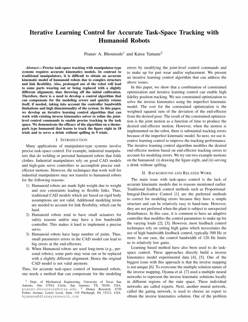
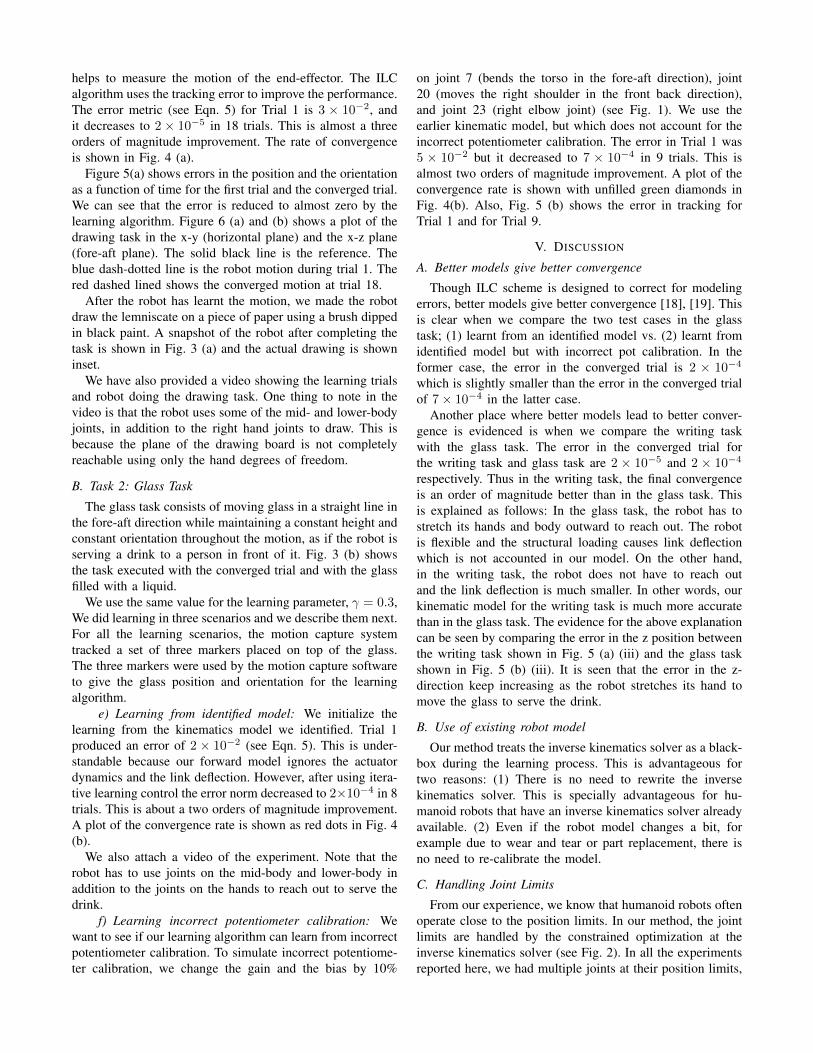
Fig. 1. (a) The kinematic model of the humanoid robot in the zero reference pose. In this pose all the joint angles zero. The robot has a total of 37actuated joints. The figure shows only 26 actuated joints and which are numbered from 1 through 26. The actuated joints not shown here are the 10 fingerjoints and 1 eye-blink joint. The joints A through E are neither sensed nor actuated. In this paper, we only use the following 14 actuated joints for control;1 through 7 in the body, and 19 through 26 in the right hand. (b) A photo of the humanoid robot that we used in this study. Gross robot specifications are:height = 1.8 m (5’11”), body width = 0.28 m (9”), and length of hand = 0.67 m (2’2”). The above pose is our reference pose for the inverse kinematics(see Sec III-C). A plastic glass is glued to the right hand of the robot and is shown inset. We put three markers on the top of the glass which we trackusing Opti-track motion capture system.

with the above method is that the construction of the gatingnetwork becomes difficult in high dimensions.

Iterative Learning Control (ILC) can make up for modelingerrors to enable high fidelity tracking. In its simplest form,ILC modifies the control command in every iteration in thefollowing way: the command at trial i, is the sum of thecommand in trial i−1, and a control gain times the trackingerror in trial i−1 [8]. Because the tracking errors are reducediteratively at every trial, the control gains can be kept small.

Traditionally, in ILC, the learning is at the joint level[10]. However, it is quite straightforward to extend ILC totask level using the appropriate mapping from the task-spaceto the joint space. For example, Arimoto et al. [11], [12]used the linearized mapping, i.e., the Jacobian, to map theincremental change in position from the task level to the jointlevel and showed the efficacy of their algorithm on a fourlink manipulator in simulation. In our ILC algorithm, we usethe non-linear map from task-space to joint space and showthe efficacy of the algorithm experimentally on a humanoid.Specifically, we evaluate the non-linear map by using aninverse kinematics solver which find solutions within thejoint limits. The main improvement over Arimoto’s algorithmis that our algorithm is able to handle joint limits [9].

III. METHODS

A. Robot hardware

We use a 37 degree of freedom, hydraulically powered,fixed-base humanoid robot shown in Fig. 1. Each joint haseither a rotary potentiometer or a linear variable differential

transformer to sense joint position. There are two levels ofcontrol. At the lowest level, there is a single processor perjoint. The processor runs a 1 KHz control loop that doeshigh gain position control using individual position data fromjoint sensor, velocity from differentiated and filtered positiondata from joint sensor and the force sensor in the valve. Thegains on the lowest level controller are pre-set and cannotbe changed. At the highest level, there is a single computerthat communicates with all the low level processors at 120Hz, sending desired joint position commands and receivingmeasured position. We control the robot at the highest levelin all experiments reported here, i.e. the input is a positioncommand and the joint position is the measured variable,both of which occur at a bandwidth of 120 Hz.

B. Marker-based motion capture

We use an 8-camera motion capture system by OptiTrack[13]. The motion capture system outputs the position and theorientation of the end-effector by measuring the position ofthe three retro-reflective markers that we place on the end-effector.

We first use the motion capture system to develop a kine-matic model of the robot. The robot joints are made to movein a random fashion and the joint position from the robotcontrol system and the end-effector position and orientationfrom the motion capture system are simultaneously recorded.Then, a kinematic model is specified and parameters arefit using non-linear least squares. The model has limitedaccuracy due to unmodeled effects such as sensor noise

and link deflection due to load. We provide more detailsin Bhounsule and Yamane [14].

We also use the motion capture system to track the end-effector motion during the task-space experiments. We usethe tracking errors in the position and the orientation in theiterative learning control algorithm which we describe indetail in Sec. III-D.

C. Inverse Kinematics

We need an inverse kinematics solver to map the desiredend-effector motion to joint space for the low level positionservo. The use of optimization based inverse kinematicssolver provides a straight-forward and generalizable methodof creating solutions for redundant robots, such as humanoidrobots [15]. Specifically, by choosing a suitable cost functionone can bias the solution to use certain joints over the otherones.

We use a constrained optimization software SNOPT [16]to develop an inverse kinematics solver. The problem hereis to find the joint angles as a function of time, θ(t),to minimize the cost function g, subject to end-effectorconstraints h1, the lower joint limits h2, and upper jointlimits h3. We define these functions next:

g(θ(t)) =

ndof∑i=1

wi(θi(t)− θrefi (t))2, (1)

h1(θ(t)) = Xdes(t)− f(θ(t)) ≤ |ε|, (2)h2(θ(t)) = θ(t)− θmin ≥ 0, (3)h3(θ(t)) = θ(t)− θmax ≤ 0. (4)

In the above scheme, we specify the desired motion of theend-effector, Xdes(t) (e.g. trajectory of the pen to draw thefigure eight). Further, we define ndof to be the degrees offreedom used by the robot in the experiment. We assumeε = 10−3.

The following are free parameters which the motion de-signer can tune in order to bias the motion.

1) The reference angles for the joints, θrefi (t). We choose,

θrefi (t) = θref

i (constant), and is the joint angles corre-sponding to the robot pose shown in Fig. 1.

2) The joint weighting wi. We intuitively chose a weightof 1 for the joints for the hand degrees of freedomand choose a weight of 10 for the joints in themid- and lower-body. This choice of this particularweight distribution has the effect of finding solutionsthat involve bigger excursions of the hand degrees offreedom than the body degrees of freedom, similar towhat humans would do when doing tasks using theirhands. Alternately, the weights can be chosen usinginverse optimization using motion capture data (e.g.,See Liu et al. [17])

D. Iterative Learning Control (ILC) Algorithm

The joint angle solution θ(t) leads to poor performancewhen we implement it on the robot because of the imperfectkinematic model. So, we implement an iterative learning

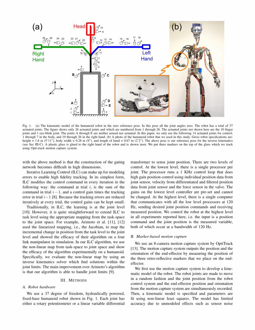
From Memory

Save To Memory

Xides (j)

ei(j)

Memory (All computations offline)

-+

Xiact(j)Xref(j)

Robot

Iterative Learning Control Update Rule

Inverse Kinematics

Xides (j) = Xi

des(j) + γ (j)-1 i -1e

θi(j)

(j)i -1e

Saved errors from i-1 trialafter filtering

Low Level Controller

vi(j)

Cartesian Error

PositionCommand

Valve Command

Fig. 2. Block diagram of our end-effector space iterative learning controlalgorithm. We filter the cartesian space errors ei−1(j) using a zero phasefilter before applying the iterative learning update rule. The super-script idenotes the trial number and j denotes a time instance.

control to improve the tracking performance of the inversekinematics solution. We describe the algorithm next.

Let i represent the trial number and j the time index thatgoes from 1 to nj (end time). Let the reference motion intask-space be defined by Xref(j). Here we have concatenatedthe position and the orientation in the vector X. The inputto the inverse kinematics solver are the desired poses inend-effector space, which we denote by Xi

des(j). Let themeasured position in task-space be defined by Xi

act(j). Letthe error between actual end-effector position and referenceposition be denoted by ei(j) = Xi

ref(j)−Xact(j). Our ILCalgorithm is shown in Fig. 2 and described below:

1) Set the error e0(j) = 0 and initialize the desiredposition in the task-space X0

des(j) = Xref(j).2) For subsequent trials do:

• Command modification in end-effector space: Up-date the feed-forward position command using thetracking error at trial i, Xi

des(j) = Xi−1des (j) +

Γei−1(j). The manually tuned learning gain, Γ, isa 6x6 matrix of the form; Γ = diag{γ1, γ2, ...γ6}.Further, for ILC to converge we need, 0 < γi ≤ 1.

• Command initialization in joint-space: For thedesired position in task-space Xi

des(j), use theinverse kinematics solver to find a desired jointcommand θi(j).

• Command execution on robot: Send the feed-forward commands θi(j) (j = 1, 2, ..., nj) tothe low level controller. Save the resulting track-ing errors in the end-effector space, ei(j) (j =1, 2, ..., nj).

3) Stop when the error metric einorm does not improvebetween trials. The learnt feed-forward command isthen θi(j) (j = 1, 2, ..., nj).

The error metric to check convergence is given as follows

einorm =1

nj

nj∑j=1

neff∑k=1

(eik(j))2, (5)

where eik(j) is the tracking error in the pose element k, atiteration i and at time j, neff = 6 and nj is the total datapoints in the trial.

E. Performance of the algorithma) System equations: The ILC update equation is:

Xides(j) = Xi−1

des (j) + Γei−1(j) (6)

Next, we linearize the output equation which relates theactual joint position, Xi

act with the control equation Xides.

Xiact(j) = f(f−1(Xi

des(j)))

= F(Xides(j))

≈ GXides(j) where G =

∂F

∂Xides

(7)

where f , f are the true model and approximate modelrespectively, F = f(f−1(.)). A first order approximation ofF has to be linearly proportional to Xi

des for the equation tobe dimensionally consistent.

b) Convergence analysis: To do convergence analysis,we need to express the error between successive trials. Thisis done as follows.

ei(j) = Xref(j)−Xiact(j)

= Xref(j)−GXides(j)

= Xref(j)−GXi−1des (j)−GΓei−1(j)

= Xref(j)−Xi−1act (j)−GΓei−1(j)

= ei−1(j)−GΓei−1(j)

= (I−GΓ)ei−1(j)

The condition for convergence is that the |ei−1(j)| < |ei(j)|.This condition is met when the eigenvalues of (I−GΓ) areless than 1.

c) Stability analysis: We simplify the ILC update equa-tion as follows:

Xides(j) = Xi−1

des (j) + Γ(Xref(j)−Xi−1act (j))

= Xi−1des (j) + ΓXref(j)− ΓGXi−1

des (j)

= (I− ΓG)Xi−1des (j) + ΓXref(j)

The condition for stabile learning is that the control com-mand, Xi

des(j) should be bounded. This happens when thewhen the eigenvalues of (I− ΓG) are less than 1.

d) Tuning the learning gain: In the previous two sec-tions, we saw that the learning gains, Γ, affects the stabilityas well as convergence. These are the only parameter thatneeds to be manually tuned in the algorithm. We simplify thisby choosing the same learning parameter for all six degreesof freedom. Thus Γ = γI , where I is 6x6 identity matrixand 0 < γ ≤ 1. The closer this value is to 1, the faster isthe convergence. But the sensor noise limits the use of highgains. A straightforward way to enable high values for γ isto filter the noisy sensor data. This is discussed next.

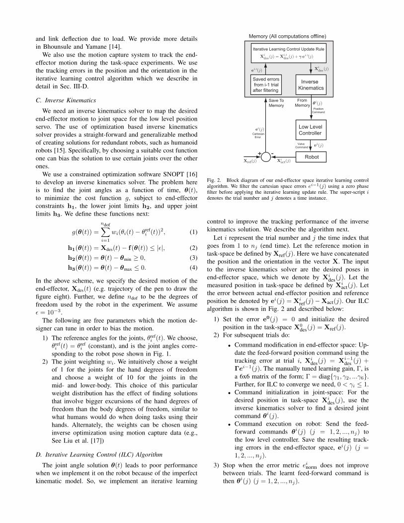
Fig. 3. (a) Robot after completing the writing task after learning. Thefigure “eight” drawn by the robot is shown inset, and (b) Robot doing theglass task after learning.

F. Zero phase filtering

We use a zero phase filter that removes sensor noise andprovides sensor data with zero phase lag. We first filter inthe forward direction using a second order Butterworth filterwith cutoff frequency of 1 Hz. Next, we pad the forwardfiltered signal with about 120 reflected data points at thebeginning and at the end. Then, we reverse the concatenatedsignal and filter again with the same Butterworth filter. Thisprocess of forward filtering followed by reverse filteringproduces a signal with zero delay. The padding of dataremoves unnecessary transients in the beginning and the endof the filtered signal. Note that the zero-phase filtering is anti-causal and it needs the sensor values for the entire trajectoryand is done offline.

IV. EXPERIMENTAL RESULTS

We show implementation of our algorithm on the hu-manoid robot shown in Fig. 1. In order to generate the results,we used the following 14 actuated joints shown in Fig. 1 (a);1 through 7 in the body, and 19 through 26 in the right hand.The joints A through E are neither sensed or actuated butneed to move in order to allow the loop joint in the lowerbody to move.

A. Task 1: Writing Task

The writing task consists drawing the lemniscate, which isthe figure eight or the ∞ symbol. We specify the lemniscateequation in Xdes(t). We use the inverse kinematic solver (seeSee III-C) to compute the joint position command θ(t)). Thejoint command is then played back on the robot. The motionof the end-effector is tracked by three markers placed on theright hand. The kinematic model does not take into accountthe actuator dynamics or the link deflection, and does notproduce error free tracking. Finally, we use the the inverseILC algorithm to improve the tracking performance.

The learning parameter γ was manually tuned to 0.3 byrunning a few trials on the robot. While the robot is learning,the robots draws in the air and the motion capture system

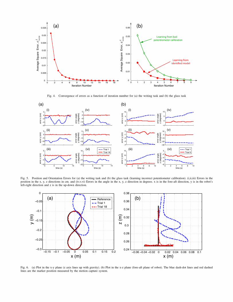
helps to measure the motion of the end-effector. The ILCalgorithm uses the tracking error to improve the performance.The error metric (see Eqn. 5) for Trial 1 is 3 × 10−2, andit decreases to 2× 10−5 in 18 trials. This is almost a threeorders of magnitude improvement. The rate of convergenceis shown in Fig. 4 (a).

Figure 5(a) shows errors in the position and the orientationas a function of time for the first trial and the converged trial.We can see that the error is reduced to almost zero by thelearning algorithm. Figure 6 (a) and (b) shows a plot of thedrawing task in the x-y (horizontal plane) and the x-z plane(fore-aft plane). The solid black line is the reference. Theblue dash-dotted line is the robot motion during trial 1. Thered dashed lined shows the converged motion at trial 18.

After the robot has learnt the motion, we made the robotdraw the lemniscate on a piece of paper using a brush dippedin black paint. A snapshot of the robot after completing thetask is shown in Fig. 3 (a) and the actual drawing is showninset.

We have also provided a video showing the learning trialsand robot doing the drawing task. One thing to note in thevideo is that the robot uses some of the mid- and lower-bodyjoints, in addition to the right hand joints to draw. This isbecause the plane of the drawing board is not completelyreachable using only the hand degrees of freedom.

B. Task 2: Glass Task

The glass task consists of moving glass in a straight line inthe fore-aft direction while maintaining a constant height andconstant orientation throughout the motion, as if the robot isserving a drink to a person in front of it. Fig. 3 (b) showsthe task executed with the converged trial and with the glassfilled with a liquid.

We use the same value for the learning parameter, γ = 0.3,We did learning in three scenarios and we describe them next.For all the learning scenarios, the motion capture systemtracked a set of three markers placed on top of the glass.The three markers were used by the motion capture softwareto give the glass position and orientation for the learningalgorithm.

e) Learning from identified model: We initialize thelearning from the kinematics model we identified. Trial 1produced an error of 2 × 10−2 (see Eqn. 5). This is under-standable because our forward model ignores the actuatordynamics and the link deflection. However, after using itera-tive learning control the error norm decreased to 2×10−4 in 8trials. This is about a two orders of magnitude improvement.A plot of the convergence rate is shown as red dots in Fig. 4(b).

We also attach a video of the experiment. Note that therobot has to use joints on the mid-body and lower-body inaddition to the joints on the hands to reach out to serve thedrink.

f) Learning incorrect potentiometer calibration: Wewant to see if our learning algorithm can learn from incorrectpotentiometer calibration. To simulate incorrect potentiome-ter calibration, we change the gain and the bias by 10%

on joint 7 (bends the torso in the fore-aft direction), joint20 (moves the right shoulder in the front back direction),and joint 23 (right elbow joint) (see Fig. 1). We use theearlier kinematic model, but which does not account for theincorrect potentiometer calibration. The error in Trial 1 was5 × 10−2 but it decreased to 7 × 10−4 in 9 trials. This isalmost two orders of magnitude improvement. A plot of theconvergence rate is shown with unfilled green diamonds inFig. 4(b). Also, Fig. 5 (b) shows the error in tracking forTrial 1 and for Trial 9.

V. DISCUSSION

A. Better models give better convergence

Though ILC scheme is designed to correct for modelingerrors, better models give better convergence [18], [19]. Thisis clear when we compare the two test cases in the glasstask; (1) learnt from an identified model vs. (2) learnt fromidentified model but with incorrect pot calibration. In theformer case, the error in the converged trial is 2 × 10−4

which is slightly smaller than the error in the converged trialof 7× 10−4 in the latter case.

Another place where better models lead to better conver-gence is evidenced is when we compare the writing taskwith the glass task. The error in the converged trial forthe writing task and glass task are 2 × 10−5 and 2 × 10−4

respectively. Thus in the writing task, the final convergenceis an order of magnitude better than in the glass task. Thisis explained as follows: In the glass task, the robot has tostretch its hands and body outward to reach out. The robotis flexible and the structural loading causes link deflectionwhich is not accounted in our model. On the other hand,in the writing task, the robot does not have to reach outand the link deflection is much smaller. In other words, ourkinematic model for the writing task is much more accuratethan in the glass task. The evidence for the above explanationcan be seen by comparing the error in the z position betweenthe writing task shown in Fig. 5 (a) (iii) and the glass taskshown in Fig. 5 (b) (iii). It is seen that the error in the z-direction keep increasing as the robot stretches its hand tomove the glass to serve the drink.

B. Use of existing robot model

Our method treats the inverse kinematics solver as a black-box during the learning process. This is advantageous fortwo reasons: (1) There is no need to rewrite the inversekinematics solver. This is specially advantageous for hu-manoid robots that have an inverse kinematics solver alreadyavailable. (2) Even if the robot model changes a bit, forexample due to wear and tear or part replacement, there isno need to re-calibrate the model.

C. Handling Joint Limits

From our experience, we know that humanoid robots oftenoperate close to the position limits. In our method, the jointlimits are handled by the constrained optimization at theinverse kinematics solver (see Fig. 2). In all the experimentsreported here, we had multiple joints at their position limits,

but the learning proceeded seamlessly, converging to a smalltracking error. We believe that this is a significant advantageof our method over methods that work at the velocity leveland use the Jacobian to map from task-space to joint space.

D. Limitations of our method

Our method has all the limitations of ILC: it is an offlinemethod; it needs manual tuning to work well; and it canonly improve a single trajectory at a time. In addition, ourmethod needs an inverse kinematics solver that is able to findsolutions within joint limits. This can be computationallyexpensive and can lead to issues if the manipulator is insingular configuration.

VI. CONCLUSIONS AND FUTURE WORK

In this paper, we present an Iterative Learning Control al-gorithm for high-fidelity tracking of end-effector motions forhigh degree of freedom manipulator system in the presenceof modeling errors. We create the given end-effector motionusing an inverse kinematics solver based on constrainedoptimization. The cost function in the optimization providesflexibility to select a motion style by appropriate choice ofreference pose and joint weights. To enable high-fidelitytracking in the presence of modeling errors, we iterativelymodifying the end-effector reference motions using the track-ing errors. These are then mapped back into joint space usingthe inverse kinematics solver. We demonstrate the efficacy ofour algorithm on a high degree of freedom humanoid robotthat iteratively learns writing the figure eight in 18 trials andlearns to move a glass in a perfectly level manner in 9 trials.

Future work will be directed towards incorporating veloc-ity limits (note that in the current work we only implementposition limits), which will help to extend this work to fastmotions.

REFERENCES

[1] K.J. Astrom, and T. Hagglund, PID Controller: Theory, Design, andTuning, International Society for measurement and Control Seattle,WA, 1995

[2] T.B.Cunha, C. Semini, E. Guglielmino, V.J. De Negri, Y.Yang, andD.G. Caldwell Gain scheduling control for the hydraulic actuationof the HyQ robot leg. Proceedings of the International Congress ofMechanical Engineering, Gramado, Brazil. 2009.

[3] D. Sun, and J.K. Mills, High-accuracy trajectory tracking of industrialrobot manipulator using adaptive-learning schemes, American ControlConference, 1999,

[4] A. Guez and Z. Ahmad. Solution to the inverse kinematics problem inrobotics by neural networks. In Neural Networks, IEEE InternationalConference on, pages 617–624. 1988.

[5] R. Koker, C. Oz, T. Cakar and H. Ekiz. A study of neural networkbased inverse kinematics solution for a three-joint robot. Robotics andAutonomous Systems, 49(3):227–234, 2004.

[6] M. I. Jordan and D. E. Rumelhart. Forward models: Supervisedlearning with a distal teacher. Cognitive science, 16(3):307–354, 1992.

[7] E. Oyama, N. Y. Chong, A. Agah, and T. Maeda. Inverse kinematicslearning by modular architecture neural networks with performanceprediction networks. In Robotics and Automation, IEEE InternationalConference on, volume 1, pages 1006–1012. IEEE, 2001.

[8] S.Arimoto, S.Kawamura, and F.Miyazaki. Bettering operation ofrobots by learning. Journal of Robotic 1(2):123-140, 1984.

[9] P. A. Bhounsule, K. Yamane and A. A. Bapat A task-level it-erative learning control algorithm for redundant manipulators withjoint position limits IEEE–International Conference on Robotics andAutomation (submitted) , 2016

[10] D. Bristow, M. Tharayil, and A. G. Alleyne, A survey of iterativelearning control Control Systems, IEEE, 26(3):96–114, 2006.

[11] S. Arimoto, M. Sekimoto and S. Kawamura. Iterative learning ofspecified motions in task-space for redundant multi-joint hand-armrobots. In Robotics and Automation, IEEE International Conferenceon, pages 2867–2873. IEEE, 2007.

[12] S. Arimoto, M. Sekimoto, and S. Kawamura. Task-space iterativelearning for redundant robotic systems: existence of a task-spacecontrol and convergence of learning. SICE Journal of Control,Measurement, and System Integration, 1:312–319, 2008.

[13] OptiTrack - ARENA - Body motion capture software for 3D char-acter animation and more. http://www.naturalpoint.com/optitrack/products/arena/, [Online; accessed 26 November2013].

[14] P. A Bhounsule and K. Yamane. Full-Pose Calibration of a HighDegree of Freedom Humanoid Robot using Marker-Based MotionCapture System. Industrial Robot: An International Journal 2015(submitted).

[15] L. T. Wang and C. C. Chen, A combined optimization method forsolving the inverse kinematics problems of mechanical manipulatorsIEEE Transaction on Robotics, vol=7, no=4, pp. 489–499, 1991.

[16] P. E. Gill, W. Murray and M. A. Saunders. Snopt: An SQP algorithmfor large-scale constrained optimization. SIAM journal on optimiza-tion, 12(4):979–1006, 2002.

[17] K. C. Liu, and A. Hertzmann, and Z. Popovic Learning physics-basedmotion style with nonlinear inverse optimization ACM Transactionson Graphics (TOG), 24(3):1071–1081, 2005.

[18] P. A. Bhounsule, and K. Yamane. Iterative Learning Control for High-Fidelity Tracking of Fast Motions on Entertainment Humanoid Robots.IEEE-RAS International Conference on Humanoid Robots, Atlanta,GA, USA, 2013.

[19] C. G. Atkeson and J. McIntyre. Robot trajectory learning throughpractice. In IEEE International Conference on Robotics and Automa-tion, volume 3, pp. 1737–1742, 1986.

0 2 4 6 8 10 12 14 16 180

0.005

0.01

0.015

0.02

0.025

0.03

0.035

Iteration Number

Aver

age

Squa

re E

rror,e

i norm Learning from bad

potentiometer calibration

Learning from identi�ed model

0 1 2 3 4 5 6 7 8 90

0.01

0.02

0.03

0.04

0.05

0.06

Iteration Number

Aver

age

Squa

re E

rror,e

i norm

(a) (b)

Fig. 4. Convergence of errors as a function of iteration number for (a) the writing task and (b) the glass task

−6

−4

−2

0

2

erro

r x (c

m)

−15

−10

−5

0

5

erro

r y (c

m)

0 5 10 15−10

−5

0

5

erro

r z (c

m)

time (s)

−15

−10

−5

0

5

−15

−10

−5

0

5

0 5 10 15−20

−10

0

10

erro

r ang

lez

(deg

rees

)

time (s)

erro

r ang

ley

(deg

rees

)er

ror a

ngle

z (d

egre

es)

Trial 1Trial 18

(i) (iv)

(ii)

(iii)

(v)

(vi)

(a) (b)

−5

0

5

10

−4

−3

−2

−1

0

0 2 4 6 8 100

5

10

15

−5

0

5

10

−30

−20

−10

0

10

0 2 4 6 8 10−8

−6

−4

−2

0

erro

r x (c

m)

erro

r y (c

m)

erro

r z (c

m)

time (s)

erro

r ang

lez

(deg

rees

)

time (s)

erro

r ang

ley

(deg

rees

)er

ror a

ngle

z (d

egre

es)

Trial 1Trial 9

(i) (iv)

(ii)

(iii)

(v)

(vi)

Fig. 5. Position and Orientation Errors for (a) the writing task and (b) the glass task (learning incorrect potentiometer calibration). (i,ii,iii) Errors in theposition in the x, y, z directions in cm. and (iv,v,vi) Errors in the angle in the x, y, z direction in degrees. x is in the fore-aft direction, y is in the robot’sleft-right direction and z is in the up-down direction.

−0.15 −0.1 −0.05 0 0.05 0.1 0.15 0.2−0.3

−0.25

−0.2

−0.15

−0.1

−0.05

x (m)

y (m

)

0

−0.06 −0.04 −0.02 0 0.02 0.04 0.06 0.08 0.10.24

0.26

0.28

0.3

0.32

0.34

0.36

0.38

x (m)

z (m

)

(a) (b)ReferenceTrial 1Trial 18

Fig. 6. (a) Plot in the x-y plane (z axis lines up with gravity). (b) Plot in the x-z plane (fore-aft plane of robot). The blue dash-dot lines and red dashedlines are the marker position measured by the motion capture system.