Contents lists available at ScienceDirect

Applied Energy

journal homepage: www.elsevier.com/locate/apenergy

Iterative multi-task learning for time-series modeling of solar panel PVoutputs

Tahasin Shireena, Chenhui Shaob, Hui Wanga,⁎, Jingjing Lic, Xi Zhangd, Mingyang Lie

a Department of Industrial and Manufacturing Engineering, Florida State University, 2525 Pottsdamer St., Tallahassee, FL 32310, USAbDepartment of Mechanical Science and Engineering, University of Illinois at Urbana-Champaign, 1206 W. Green St., Urbana, IL 61801, USAc Department of Industrial and Manufacturing Engineering, Pennsylvania State University, 310 Leonhard Building, University Park, PA 16802, USAd Department of Industrial Engineering and Management, Peking University, 298 Chengfu Rd., Beijing 100871, Chinae Department of Industrial and Management Systems Engineering, University of South Florida, Tampa, FL 33620, USA

H I G H L I G H T S

• An improved method for solar panel PV generation prediction is developed.

• Fusion of PV data from similar solar panels can significantly improve PV prediction.

• The multi-task learning algorithm is improved and generalized for time-series data.

• Systematic discussions and guidelines for implementation of the method are provided.

A R T I C L E I N F O

Keywords:Multi-task learningTime seriesSolar panelsPredictionForecasting

A B S T R A C T

Time-series modeling of PV output for solar panels can help solar panel owners understand the power systems’time-varying behavior and be prepared for the load demand. The time-series forecast/prediction can becomechallenging due to many missing observations or a lack of historical records that are not sufficient to establishstatistical models. Increasing PV measurement frequency over a longer period increases the cost in the detectionof the PV fluctuation. This paper proposes an efficient approach to iterative multi-task learning for time series(MTL-GP-TS) that improves prediction of the PV output without increasing measurement efforts by sharing theinformation among PV data from multiple similar solar panels. The proposed iterative MTL-GP-TS model learns/imputes unobserved or missing values in a dataset of time series associated with the solar panel of interest topredict the PV trend. Additionally, the method improves and generalizes the traditional multi-task learning forGaussian Process to the learning of both global trend and local irregular components in time series. A real-worldcase study demonstrated that the proposed method could result in substantial improvement of predictions overconventional approaches. The paper also discusses the selection of parameters and data sources when im-plementing the proposed algorithm.

1. Introduction

Photovoltaic (PV) output is one of the most critical performanceindicators for solar panels. The PV forecast/prediction can help solarpanel owners be prepared for load demand and efficiently supply thesolar energy as a complimentary source for power grids, withoutoverestimating or underestimating the capabilities of solar panels.Additionally, the temporal prediction can help detect potential ab-normal PV variations in a timely manner. Modeling of the PV timeseries usually employs statistical methods to progressively predict thePV output over time in near future based on the trend as reflected in

historical data, which is collected at a specified time interval. The time-series model requires sufficient training data to establish adequatestatistical confidence.

As reviewed in [1], there has been a noticeable amount of researchon forecasting time-series data in solar panels and solar radiation in-cluding ARMA (Auto-regressive and Moving Average), ARIMA (auto-regressive integrated moving average) [2]. Time-series modeling alsoconsiders the impact of environmental factors on the PV outputs basedon ARMAX (autoregressive-moving-average model with exogenous in-puts) [3,4]. In [5], artificial neural networks with multi-layer percep-tron were developed to forecast the daily solar radiation in time-series

https://doi.org/10.1016/j.apenergy.2017.12.058Received 30 July 2017; Received in revised form 5 December 2017; Accepted 9 December 2017

⁎ Corresponding author.E-mail address: hwang10@fsu.edu (H. Wang).

Applied Energy 212 (2018) 654–662

Available online 22 December 20170306-2619/ © 2017 Elsevier Ltd. All rights reserved.

T

dataset by using transfer function of hidden layers. Almeida et al. [6]presented another forecasting approach with a nonparametric model ofAC power forecast with quantile regression forests as machine learningtools. The research of the forecast with nonparametric approaches arefound in [7,8] to forecast short-term PV outputs. A hybrid method usingsupport vector machine with firefly algorithm was introduced by [9] toforecast the solar radiation. Time series modeling has also been appliedto other green energy generation such as wind power forecasting[10–12].

One of the major challenges in the time-series modeling of PVoutput for a solar panel is missing data or data gaps due to a variety ofreasons. Data collection may be interrupted due to technical problemssuch as data measurement equipment failure, erroneous recordings,weather factors. The problem of missing historical data is particularlysignificant for a newly deployed solar panel system. As a result, thereexist substantial gaps in data collection for time-series modeling and themissing values in time series can cause a poor prediction of PV output.Increasing the measurement frequency of PV data or collecting moremeasurements over a longer period adds to the measurement cost.Therefore, it is essential to develop an efficient way to improve theperformance prediction of the solar panel trend when there are manymissing-value gaps in the training data for statistical modeling.

The effects of missing observations on the predicted result havebeen studied by various research. The missing observations in timeseries dataset can be dealt with by the following two approaches, i.e.,

1. Interpolation and extrapolation methods. Example approaches in-clude linear interpolation, AR predictor [13], autoregressive con-ditionally heteroscedastic [14], Kalman filtering [15], neural net-works [16] and multiple imputation models discussed in [17].Techniques were also developed to reduce sampling rate or timeresolution for PV time-series modeling [18]. This line of researchcan help smooth the prediction data, but nevertheless does not ne-cessarily improve the prediction/forecast accuracy due to the lim-ited useful information added to the time-series modeling.

2. Incorporation of environmental factors. The problem of predictingthe time series response PV t( ) can be mitigated by fusing the effectof historical environmental data such as temperature, wind speed,and humidity in ARMAX, artificial intelligent (AI) model includingANN (artificial neural network) [1,19,20], wavelet-coupled supportvector machine model [21], and analog ensemble method [22]. Thehistorical PV data such as − − − …PV t PV t PV t( 1), ( 2), ( 3) in thesemodels can be de-seasoned by deducting the effect of solar irra-diance IR t( ) via − − = …PV t k IR t k k( )/ ( ), 1,2,3 . It can be seen that thehistorical PV responses are one of the most significant variables thataffect the forecasting/prediction performance based on the de-sea-soned data. As such, improving the imputation of historical PV datais highly beneficial for time series modeling.

Time-series modeling based on these methods is considered as singletask learning (STL) because the learning is accomplished by using thedata from one single source, i.e., the solar panel of interest. Due to thelimitation of information sources, such STL offers limited improvementin learning missing values to capture the true PV trend when there aremany missing values.

A new opportunity emerges in improving the learning of the un-observed values by sharing the knowledge or information availablefrom other data collected under similar conditions. For example, whena solar panel may not have sufficient data to estimate its performancesuch as a new PV system, the history of an old solar panel of the sametype under similar deployment conditions can potentially provide crossinference about this panel. To enable such a knowledge transfer, amachine learning framework called multi-task learning (MTL) has beendeveloped, which learns multiple tasks simultaneously with the keyidea of sharing the information of each task [23]. The term “task” refersto the learning and prediction of certain target performance based on

data. Joint learning for all tasks using MTL can significantly mitigateproblems such as overfitting and unstable search due to sparse trainingdata while improving performance compared to STL methods [24].Relatedness among tasks is vital in MTL [25] as unrelated or dissimilartasks can be detrimental to effective learning resulting in a negativetransfer of information [26]. By utilizing the task similarity, the MTLalgorithm has been applied to a Gaussian process (GP) for spatial databased on joint priors in [26–30]. In the past, the scope of the MTL hasalso been explored in [31,32] for classification problems, in [33] forlearning using task-specific features and in [34] for learning with theinformative vector machines by learning parameters based on the ideaof task relatedness. The scope of MTL is yet to be explored in time seriesfeatures for forecasting.

Based on the review, we identified two research gaps, i.e.,

1. The traditional STL has demonstrated its effectiveness in short-termPV prediction but has its limitations when dealing with a significantamount of missing values.

2. The traditional MTL-GP method has its limitations in time-seriesmodeling for PV data. We conclude that a joint learning methodusing multiple similar-but-not-identical datasets has the potential inimproving learning/imputation of missing values and prediction ofsolar panel performance. However, the prior research on MTL for GPmostly dealt with spatial data without considering both local tem-poral dependence and global trend. To the best of our knowledge,there exists little research that explores the values of the MTL-GPmethod and improves this method in time-series modeling for PVdata.

To overcome the challenge, this paper proposes an approach toimproving prediction of solar panel performance by sharing commoninformation among similarly related time series datasets at multiplelocations. An iterative multi-task learning Gaussian process time series(MTL-GP-TS) algorithm is developed to learn the missing observationsin time series dataset without increasing measurement efforts. The term”iterative” refers to the implementation of MTL procedures in aniterative manner to gradually update the trend and local component inthe model. Specifically, an initial value will be proposed for the trend,and multi-task learning will be implemented to estimate the localcomponents. The MTL-learned local components will be used to updatethe trend. The updating procedure continues until the estimation errorconverges. We demonstrate the proposed iterative MTL-GP-TS methodusing a real-world case study based on the data collected from fourHawaiian schools. The paper also discusses two practical issues whengeneralizing the applications of the proposed algorithm.

The paper consists of the following sections. Section 2 describes theiterative MTL-GP-TS algorithm to learn unobserved values from thetime series dataset of multiple solar panels. Section 3 presents a real-world case study based on the PV data from four Hawaiian schoolsdemonstrating the iterative MTL-GP-TS method. A discussion on im-plementing the algorithm is given in Section 4. Section 5 summarizesthe paper.

2. Development of the iterative MTL-GP-TS algorithm

The MTL algorithm for GP is first reviewed in Section 2.1 following[27,28], and the iterative MTL-GP-TS algorithm is proposed in Section2.2. It should be noted that we use the term ”estimation” in this paperas the process of finding an approximated value for the model para-meters and output. We also use the term ”learning” as the process ofgaining insights through making predictions or estimation on data. Thetwo terms are used interchangeably to avoid word repetition in thispaper. The term ”prediction” is used for statistical assessment of thevalues in final outputs that have not been measured or may happen inthe future.

T. Shireen et al. Applied Energy 212 (2018) 654–662

655

2.1. A review of multi-task learning for Gaussian process

MTL formulation for Gaussian Processes. Assume that the data givenas a set of responses ∊ p( )1

1 , …, ∊ ∊p p( ), ( )N1 2

1 , …, ∊ p( )N2 ,…∊ p( )M1 , …,

∊ p( )MN , for learning M tasks at different inputs …p p pN, 2,1 , where ∊ p( )l

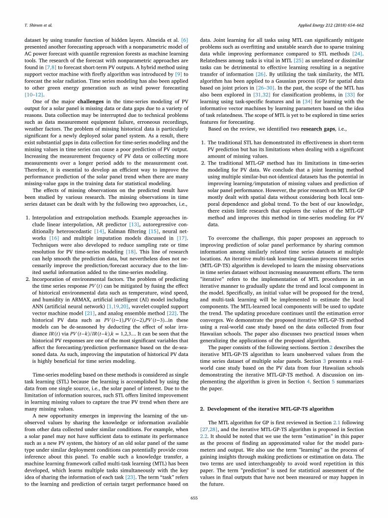
iis the response for the lth task given the ith input pi. The problem ofmulti-task learning is to predict an observed response given an input pfor a certain task based on the information from all tasks (Fig. 1). By[27,28], the response is assumed to be generated from a function ofinput p, which follows a multivariate Gaussian distribution with acovariance function κ p p( , )i j between the responses at input pi and pj(defined as a Gaussian process). Yu et al. [27] used standard equationsfor prediction using the Gaussian process to estimate the prediction atany input p by ∊ = ∑p γ κ p p( ) ( , )l

i il

i , which estimates the response at p asa linear combination of kernel values κ p p( , )i j . The coefficients, γi

l, areassumed to follow a normal distribution ∼γ N μ C( , )i

lγ γ . The distribution

parameters are assumed to jointly follow a normal-inverse-Wishart

distribution as ∼ −( )μ C μ C C τ κ( , ) 0, ( | , )γ γ γ π γ γ1 1N IW , and π and τ

are parameters in the distributions. Given the hyper prior distributionof μ C,γ γ, Yu et al. [27] further proposed a data prediction model underthe MTL framework as follows

1. Parameters μγ and Cγ are generated (or statistically sampled) foronce based on the normal-inverse-Wishart distribution

2. At a certain input p,

∑∊ = +p γ κ p p e( ) ( , ) ,l

iil

i(2.1)

where ∼e N σ(0, )2 .

The estimates of parameters μ C σ, ,γ γ and γil can be learned by an

Expectation-Maximization (EM) algorithm. The details about the EMalgorithm is reviewed in Appendix B.

MTL for solar panel PV forecasting. When the MTL model is appliedto the PV data forecasting for solar panels, ∊ p( )l

i can represent PV-re-lated output variable for the solar panel at the location of interest. Indexp becomes a time index, and we replace it with a notation t for MTL oftime-series data in the remainder of this paper. The PV-related outputvariable can be chosen as PV, PV regularized by solar irradiance, or alocal component in the PV data (see details in Section 2.2). As such, theMTL problem aims to estimate the PV-related output of the solar panelat the location of interest (target) by aggregating the similarity betweenthe solar panel’s PV output at a time point i (including those solar

panels at different locations) and the target. The similarity betweendifferent solar panels are captured by the kernel function κ and itsstrength is reflected by coefficient γi

l.The limitation of the traditional MTL-GP method is that the ap-

proach lacks the capability of capturing the temporal trend in data,which are critical for temporal data modeling. Specifically, the tradi-tional MTL-GP method only predicts the spatial data in a local model(by which data can only be estimated from those surrounding it, such asa Gaussian Process model) by borrowing the information from otherspatial datasets. For the challenge in this paper, MTL needs to estimatethe parameters for both local model and a trend, which is separatedfrom the local model. However, the traditional MTL-GP cannot distin-guish the trend from the local model. Additionally, the requirement ofGaussian-distribution assumption in the MTL-GP method is not mostlyappropriate for PV data with significant trending patterns. This paperwill enhance the MTL-GP method to characterize both global trend andlocal variations in time series data for solar panels.

2.2. Improved method: iterative multi-task learning Gaussian process fortime series (MTL-GP-TS)

The time series data can be decomposed into a trend T (includingseasonal component) and an irregular/random component ∊, i.e.,

= + ∊Z t T t t( ) ( ) ( ). The irregular or random component can usually beassumed to follow a Gaussian process plus noise. The reasons forchoosing the Gaussian process are that (1) The local irregular compo-nent in time series usually exhibit strong temporal correlation or localdependency. The Gaussian process is a local modeling method, whichpredicts the outcome based on the value surrounding it by using thelocal dependency as learned from data; and (2) When the trend can becorrectly captured by the model, the left-over residual should be acorrelated stochastic process. The multivariate normal (Gaussian) dis-tribution is a very common model to characterize the statistical attri-butes of the residual stochastic process. As such, the MTL-GP method issuitable to transfer the information among irregular components fromsimilar time series datasets to the dataset of interest (target). However,learning accuracy of the irregular components using MTL-GP is greatlyinfluenced by the way how the trend and irregular components aredecomposed. Thus, joint consideration of the trend estimation andlearning of the irregular components poses a new challenge.

To fill the gap, this paper develops an iterative MTL-GP-TS algo-rithm that simultaneously estimates the trend and irregular componentthrough information transfer among datasets. The estimation procedure

Fig. 1. The framework of multi-task learning.

T. Shireen et al. Applied Energy 212 (2018) 654–662

656

is described as follows.Iterative MTL-GP-TS algorithm:

1. Start with initial time series data Z t( )l0 of size ( ×n 1), where

= …l 1,2,3 indicates data source or task, i.e., different solar panels;2. Clean the raw data to generate sorted data Z t( )s

l by removing out-liers and replacing them using the estimates based on a K-NearestNeighbors (KNN) method. Details about the KNN method are re-viewed in Appendix C;

3. Randomly select data points from Z t( )sl during a time period to

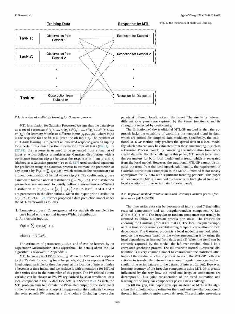
create the training dataset and the rest data during this period formthe testing dataset to simulate “missing observations.” The valida-tion dataset is formed using those observations after the period tovalidate the forecasted values for future data. The separation of thedatasets are summarized in Fig. 2;

4. Provide an initial estimate of testing datasets (that simulate“missing observations”), Z t( )l , by a linear interpolation based onthe training dataset;

5. Set =i 0 for the iteration index and =T t( ) 0l0 ∀ t for initialization;

6. Estimate irregular component, ∊ t( )il , which is assumed to follow

Gaussian process, by a decomposition, i.e., ∊ t( )il = −Z t T( )l

il(t);

7. Estimate the irregular component using MTL-GP algorithm given∊ = …t l( ), 1,2,3il from all data sources, denoted as ∊ t( )iM

l . The MTLprocedure includes (1) setting the initial values for μ C,γ γ, and γ ,which will be used for the first iteration of EM and (2) using the EMalgorithm (Appendix A) to estimate μ C,γ γ , and γ .

8. Estimate the output value by = + ∊Z t T t( ) ( )il

il

iMl ;

9. When iteration >i 1, check if ▵ = <− −−

RMSE δ| |% | |%iRMSE RMSE

RMSEi i

i1

1,

where RMSEi is the root-mean-square error calculated by com-paring the predicted output Z t( )i

l with true value Z t( )l0 in the raw

training dataset at the ith iteration and δ assumes a very smallvalue. If yes, the result converges, the final trend T t( )f

l is obtained,and we can exit the iteration. If no or when iteration index ≤i 1,update the trend by subtracting ∊ t( )iM

l from Z t( )l and then applyinterpolation to learn +T t( )i

l1 ;

10. Go to next iteration by ← +i i 1 and start with step 4;11. Conduct parameter selection based on the steps above to identify

the appropriate hyperparameters in the model (Discussed in Section4.1);

12. Conduct data source selection based on the steps above to find thedatasets to be included for the learning (Discussed in Section 4.2).

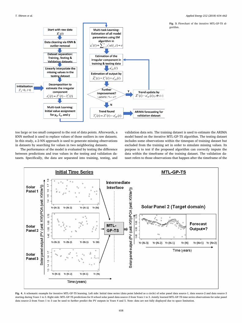
The flowchart of the procedure is summarized in Fig. 3. A timeseries model such as ARIMA can be fitted to the final estimated trendT t( )fl via the iterative MTL-GP-TS to predict future performance. It

should be noted that smooth moving average (SMA) method can beapplied for the trend estimation to mitigate the effect of noise inducedby measurement and/or weather factors.

The rationale of the proposed algorithm is as follows. The iterativemethod is used to deal with a challenge on simultaneous estimation ofboth trend and local irregular components in the time series data. Inthis problem formulation, the local irregular components can belearned through multi-task learning (MTL) based on the similaritieswith the solar panels at other locations. The iterative approach is alogical way to gradually learn about the two terms by first tentativelyestimating the local component through MTL based on initial valuesand then updating the trend and local component until convergenceafter several iterations.

Remark: The determination of the necessary data points or samplesize sufficient for the multi-task learning should be judged by howmuch the algorithm can improve the prediction accuracy (RMSE). Asthe sample size increases, the prediction performance of multi-tasklearning and STL both improve and RMSE improvement by the iterativemulti-task learning compared with the traditional STL is expected toincrease first and then approximate asymptotically to a stable constantwhen the sample size grows large. Therefore, the amount of RMSEimprovement becomes bounded and the benefits brought by multi-tasklearning thus become limited when the sample size is relatively large.

3. A case study on four Hawaiian schools

The iterative MTL-GP-TS method is demonstrated using a case studybased on solar panel datasets consisting of photovoltaic output (PV,unit: kilowatts) and plane of array (POA, unit: kilowatts per squaremeter) irradiance from four schools in Hawaii.1 The data were collectedusing “Schott Solar SunTrack Local” data acquisition system. The datafrom four school locations are selected as the input to the iterative MTL-GP-TS algorithm based on the fact that these solar panels are suppliedby the same manufacturer (i.e., SunPower SPR-200-BLK PV modules)and expected to exhibit similar variation patterns that enable theknowledge transfer across solar panels.

Remark: The distance between school locations does not play adominant role that impacts the prediction results. The key to the pre-diction is if the data at different locations may exhibit similar variationpatterns. In Section 4.1, this paper provides a data source selectionmethod that allows for judgment on whether or not a location can beincluded in the prediction.

The data sources are from Nanakuli High and Intermediate school(N), Jarrett Middle school (J), Highlands Intermediate school (H), andWaianae High school (W). All data sources show a strong positivecorrelation between the PV and POA value. Such variation patternsinduced by POA changes could potentially mask the abnormal patternsthat are associated with the intrinsic problems in solar panels, whichusers expect to detect. The removal of the POA induced effect in datacan better expose the variation patterns due to potential problems inthe solar panels. Thus, the ratio of PV over POA (i.e., PV POA/ ) is usedas time series observations to suppress the effect of POA. After re-moving the POA induced variation, the data still exhibit cyclic patternsfor time series modeling. The solar panel PV data for “H school” is to beforecast, and the rest of schools (N, J, W) supply complementary datafor multi-task learning.

The data are recorded daily and collected from Jan’2008 toApril’2012 for the four schools (N, J, H, and W). The scope of the studyis to predict the PV performance of solar panels over days and months.Although this study deals with a relatively long-term forecasting, themethodology is applicable for short-term PV forecasting as well. Thedata from Jan’2008 to April’2012 contained some inaccurate mea-surements and missing observations for some months. Outliers inducedby inaccurate measurements are removed using Tukey’s approach whilespecifying reasonable cleaning parameter that ensures no data point is

Fig. 2. An illustration of training, testing, and validation datasets. Data are randomlyselected and removed from the original data to simulate the “missing values.” These datacreate a testing dataset (white bar). The proposed iterative MTL-GP-TS algorithm is ap-plied to the training datasets (black bar) and thereby estimate the missing values corre-sponding to the time period of the testing dataset. The validation dataset (grey bar) isobtained from a future period after training and testing datasets. The training and esti-mated testing data are jointly used to fit an ARIMA time series model to estimate thefuture values corresponding to the validation dataset. The estimation for the future periodwill be compared with the values in the validation dataset to evaluate forecasting per-formance.

1 The data source is available at http://www.hawaiianelectric.com/heco/_hidden_Hidden/EducationAndConsumer/Sun-Power-for-Schools?cpsextcurrchannel=1.

T. Shireen et al. Applied Energy 212 (2018) 654–662

657

too large or too small compared to the rest of data points. Afterwards, aKNN method is used to replace values of those outliers in raw datasets.In this study, a 2-NN approach is used to generate missing observationsin datasets by searching for values in two neighboring datasets.

The performance of the model is evaluated by testing the differencebetween predictions and true values in the testing and validation da-tasets. Specifically, the data are separated into training, testing, and

validation data sets. The training dataset is used to estimate the ARIMAmodel based on the iterative MTL-GP-TS algorithm. The testing datasetincludes some observations within the timespan of training dataset butexcluded from the training set in order to simulate missing values. Itspurpose is to test if the proposed algorithm can correctly impute thedata within the timeframe of the training dataset. The validation da-taset refers to those observations that happen after the timeframe of the

Fig. 3. Flowchart of the iterative MTL-GP-TS al-gorithm.

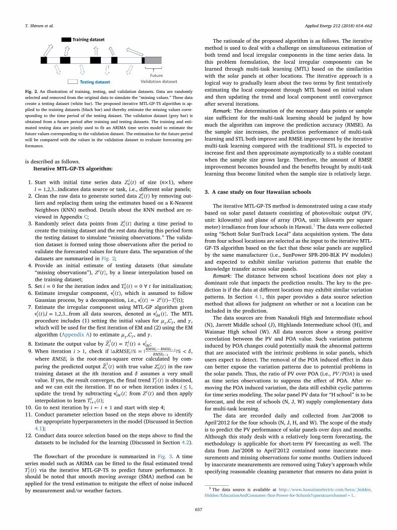
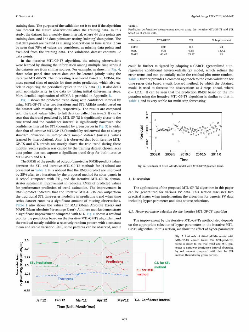
Fig. 4. A schematic example for iterative MTL-GP-TS learning. Left side: Initial time series (data point labeled as a circle) of solar panel data source-1, data source-2 and data source-3starting during Years 1 to 3. Right side: MTL-GP-TS predictions for H school solar panel data source-2 from Years 1 to 3. Jointly learned MTL-GP-TS time series observations for solar paneldata source-2 from Years 1 to 3 can be used to further predict the PV outputs in Years 4 and 5. Note: data are not fully displayed due to space limitation.

T. Shireen et al. Applied Energy 212 (2018) 654–662

658

training data. The purpose of the validation set is to test if the algorithmcan forecast the future observations after the training data. In thisstudy, the dataset has a weekly time interval, where 44 data points aretraining data, and 144 data points are testing (missing) data points. Thetest data points are treated as missing observations in time series. It canbe seen that 75% of values are considered as missing data points andexcluded from the training data. The validation dataset contains 17data points.

In the iterative MTL-GP-TS algorithm, the missing observationswere learned by sharing the information among multiple time series ifthe datasets are from similar sources. For example, as shown in Fig. 4,three solar panel time series data can be learned jointly using theiterative MTL-GP-TS. The forecasting is achieved based on ARIMA, themost general class of models for time series prediction, which also ex-cels in capturing the periodical cycles in the PV data [1]. It also dealswith non-stationarity in the data by taking initial differencing steps.More detailed explanation of ARIMA is provided in Appendix B.

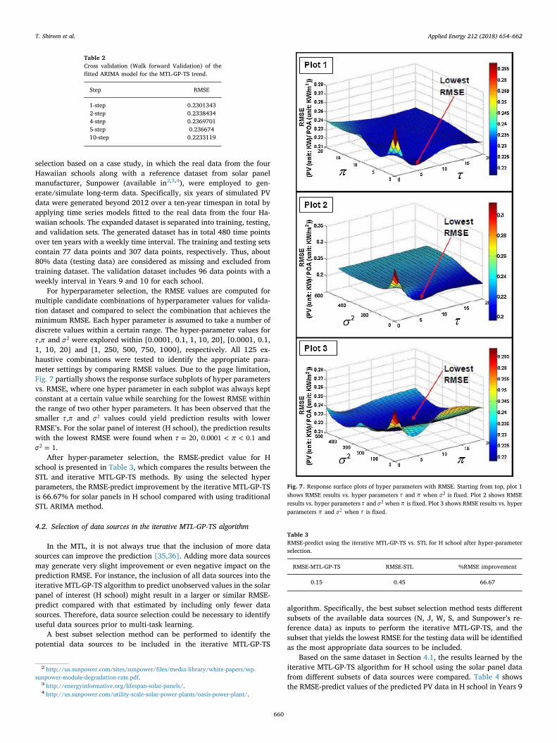
Fig. 5 shows the predicted trend along with confidence interval byusing MTL-GP-TS after two iterations and STL ARIMA model based onthe dataset with missing data, respectively. The results are comparedwith the trend values fitted to full data (as called true trend). It can beseen that the trend predicted by MTL-GP-TS is significantly closer to thetrue trend and the confidence interval is significantly narrower. Theconfidence interval for STL (bounded by green curves in Fig. 5) is widerthan that of iterative MTL-GP-TS (bounded by red curves) due to a largestandard deviation in interpolated sample dataset (missing valueslearned by interpolation). Also, it is observed that both iterative MTL-GP-TS and STL trends are mostly above the true trend during thesemonths. Such a pattern was caused by the training dataset chosen lacksdata points that can capture a significant trend drop for both iterativeMTL-GP-TS and STL.

The RMSE of the predicted output (denoted as RMSE-predict) valuesbetween the STL and iterative MTL-GP-TS methods for H school arepresented in Table 1. It is noticed that the RMSE-predict are improvedby 25% after two iterations by the proposed method for solar panels inH school compared with STL, and the iterative MTL-GP-TS demon-strates substantial improvement in reducing RMSE of predicted valuesfor performance prediction of trend estimation. The improvement inRMSE-predict indicates that the iterative MTL-GP-TS can outperformthe traditional STL time-series modeling in predicting trend when timeseries dataset contains a significant amount of missing observations.Table 1 also shows the values for MAE (Mean Absolute Error) andMAPE (Mean Absolute Percentage Error). All these metrics demonstratea significant improvement compared with STL. Fig. 6 shows a residualplot for the prediction based on the iterative MTL-GP-TS algorithm, andthe residual mostly exhibits a relatively random pattern with a constantmean and stable variation. Still, some patterns can be observed, and it

could be further mitigated by adopting a GARCH (generalized auto-regressive conditional heteroskedasticity) model, which refines theerror terms and can potentially make the residual plot more random.Table 2 further provides a common approach to the cross-validation fortime series data based a walk forward method, by which the obtainedmodel is used to forecast the observations at k steps ahead, where= …k 1,2,3 . It can be seen that the prediction RMSE based on the im-

putation using the iterative MTL-GP-TS algorithm is similar to that inTable 1 and is very stable for multi-step forecasting.

4. Discussion

The applications of the proposed MTL-GP-TS algorithm in this papercan be generalized for various PV data. This section discusses twopractical issues when implementing the algorithm for generic PV dataincluding hyper-parameter and data source selections.

4.1. Hyper-parameter selection for the iterative MTL-GP-TS algorithm

The improvement by the iterative MTL-GP-TS method also dependson the appropriate selection of hyper-parameters in the iterative MTL-GP-TS algorithm. In this section, we show the effect of hyper-parameter

Fig. 5. Residuals of fitted ARIMA model withMTL-GP-TS learned trend. The MTL-predictedtrend is closer to the true trend and MTL gen-erates a narrower confidence interval (boundedby red curves) compared with that by STLmethod (bounded by green curves).

Table 1Prediction performance measurement metrics using the iterative MTL-GP-TS and STLbased on H school data.

Metrics MTL-GP-TS STL % Improvement

RMSE 0.38 0.5 24MAE 0.31 0.38 18.42MAPE 40.47 53.97 25

Fig. 6. Residuals of fitted ARIMA model with MTL-GP-TS learned trend.

T. Shireen et al. Applied Energy 212 (2018) 654–662

659

selection based on a case study, in which the real data from the fourHawaiian schools along with a reference dataset from solar panelmanufacturer, Sunpower (available in2,3,4), were employed to gen-erate/simulate long-term data. Specifically, six years of simulated PVdata were generated beyond 2012 over a ten-year timespan in total byapplying time series models fitted to the real data from the four Ha-waiian schools. The expanded dataset is separated into training, testing,and validation sets. The generated dataset has in total 480 time pointsover ten years with a weekly time interval. The training and testing setscontain 77 data points and 307 data points, respectively. Thus, about80% data (testing data) are considered as missing and excluded fromtraining dataset. The validation dataset includes 96 data points with aweekly interval in Years 9 and 10 for each school.

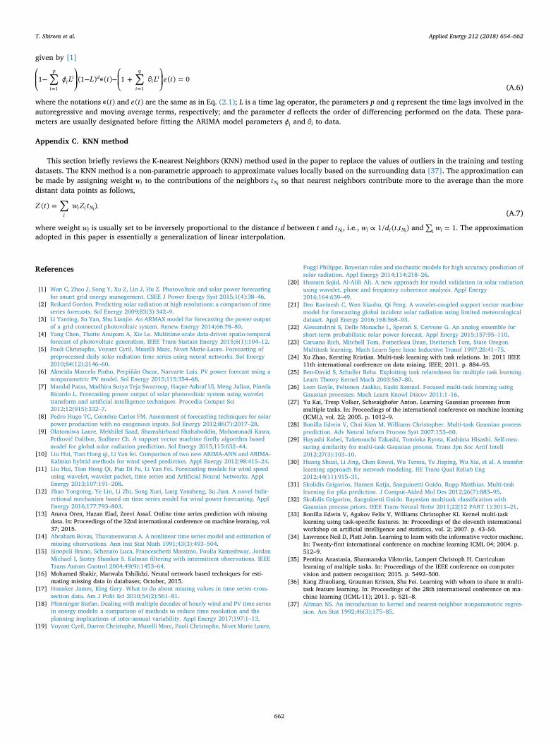
For hyperparameter selection, the RMSE values are computed formultiple candidate combinations of hyperparameter values for valida-tion dataset and compared to select the combination that achieves theminimum RMSE. Each hyper parameter is assumed to take a number ofdiscrete values within a certain range. The hyper-parameter values forτ π, and σ2 were explored within [0.0001, 0.1, 1, 10, 20], [0.0001, 0.1,1, 10, 20] and [1, 250, 500, 750, 1000], respectively. All 125 ex-haustive combinations were tested to identify the appropriate para-meter settings by comparing RMSE values. Due to the page limitation,Fig. 7 partially shows the response surface subplots of hyper parametersvs. RMSE, where one hyper parameter in each subplot was always keptconstant at a certain value while searching for the lowest RMSE withinthe range of two other hyper parameters. It has been observed that thesmaller τ π, and σ2 values could yield prediction results with lowerRMSE’s. For the solar panel of interest (H school), the prediction resultswith the lowest RMSE were found when =τ 20, < <π0.0001 0.1 and

=σ 12 .After hyper-parameter selection, the RMSE-predict value for H

school is presented in Table 3, which compares the results between theSTL and iterative MTL-GP-TS methods. By using the selected hyperparameters, the RMSE-predict improvement by the iterative MTL-GP-TSis 66.67% for solar panels in H school compared with using traditionalSTL ARIMA method.

4.2. Selection of data sources in the iterative MTL-GP-TS algorithm

In the MTL, it is not always true that the inclusion of more datasources can improve the prediction [35,36]. Adding more data sourcesmay generate very slight improvement or even negative impact on theprediction RMSE. For instance, the inclusion of all data sources into theiterative MTL-GP-TS algorithm to predict unobserved values in the solarpanel of interest (H school) might result in a larger or similar RMSE-predict compared with that estimated by including only fewer datasources. Therefore, data source selection could be necessary to identifyuseful data sources prior to multi-task learning.

A best subset selection method can be performed to identify thepotential data sources to be included in the iterative MTL-GP-TS

algorithm. Specifically, the best subset selection method tests differentsubsets of the available data sources (N, J, W, S, and Sunpower’s re-ference data) as inputs to perform the iterative MTL-GP-TS, and thesubset that yields the lowest RMSE for the testing data will be identifiedas the most appropriate data sources to be included.

Based on the same dataset in Section 4.1, the results learned by theiterative MTL-GP-TS algorithm for H school using the solar panel datafrom different subsets of data sources were compared. Table 4 showsthe RMSE-predict values of the predicted PV data in H school in Years 9

Table 2Cross validation (Walk forward Validation) of thefitted ARIMA model for the MTL-GP-TS trend.

Step RMSE

1-step 0.23013432-step 0.23384344-step 0.23697015-step 0.23667410-step 0.2233119

Fig. 7. Response surface plots of hyper parameters with RMSE. Starting from top, plot 1shows RMSE results vs. hyper parameters τ and π when σ2 is fixed. Plot 2 shows RMSEresults vs. hyper parameters τ and σ2 when π is fixed. Plot 3 shows RMSE results vs. hyperparameters π and σ2 when τ is fixed.

Table 3RMSE-predict using the iterative MTL-GP-TS vs. STL for H school after hyper-parameterselection.

RMSE-MTL-GP-TS RMSE-STL %RMSE improvement

0.15 0.45 66.67

2 http://us.sunpower.com/sites/sunpower/files/media-library/white-papers/wp-sunpower-module-degradation-rate.pdf.

3 http://energyinformative.org/lifespan-solar-panels/.4 http://us.sunpower.com/utility-scale-solar-power-plants/oasis-power-plant/.

T. Shireen et al. Applied Energy 212 (2018) 654–662

660

and 10 when using five, four and three data sources. By combining theresults in Tables 3 and 4, it can be seen that the inclusion of three datasources (N, J, and H schools) from four schools can yield a substantialimprovement in PV value prediction. However, the inclusion of allschools and manufacturer (Sunpower) reference data into the learningdoes not improve the prediction. In fact, the RMSE-predict even slightlyincreases. Thus, N, J, and H schools are sufficient for the iterative MTL-GP-TS algorithm.

5. Conclusion

This paper identifies and explores the value of diversely recorded PVdata for solar panels of similar types over a living or working area.Specifically, a new data fusion method based on multi-task learning isproposed for improving time series data imputation and prediction ofPV output of solar panels without increasing measurement efforts. Themethod overcomes the challenge in time series data modeling when asignificant amount of historical data are missing or unavailable bysharing information from other similar-but-not-identical time series. Inaddition, the proposed MTL-GP-TS algorithm generalizes the existingMTL method for Gaussian spatial processes to the learning of both

global trend and local irregular components in time series data in aniterative manner. The algorithm was applied to predict PV data overtime for solar panels deployed in four Hawaiian schools. The real-worldcase study demonstrated that the iterative MTL-GP-TS method couldefficiently learn the unobserved values in time series dataset, resultingin improved predictions of PV time series for solar panels. Parameterselection was conducted to identify appropriate hyper parameters. Ithas also been found that the performance of the proposed algorithmdepends on the selection of solar panel data sources and therefore datasource selection is necessary. The outcome of this research can help on-time preparations for load demand and assessment of solar panel con-ditions. The method can also be applicable to health condition predic-tion and missing data imputation for a wide range of applications suchas construction structures and mechanical/electronic devices. The fu-ture study involves (1) consideration of weather condition into theproposed algorithm and (2) time series model refinement to better in-corporate the data volatility by considering the variation in the errorterm such a Garch model.

Acknowledgment

This research was conducted at the High-Performance MaterialsInstitute at Florida State University. It has been partially supported by agrant from National Science Foundation (USA) CMMI-1434411 and1744131. The authors would like to thank Sun Power for SchoolsProgram hosted by Hawaiian Electric Companies, State of HawaiiDepartment of Education and Members of the community for the solarpanel installation and data collection. Assistance given by Mr. SteveLuckett from Hawaiian Electric Co Inc. was also greatly appreciated.

Appendix A. EM Algorithm

This section reviews the Expectation-Maximization (EM) algorithm used to estimate the parameters in the model = μ σΘ C{ , , }γ γ2 . The EM al-

gorithm involves an iterative procedure that alternates between an expectation step, and a maximization step. Details about the EM algorithm hasbeen documented in [27].

• Expectation, E-step: This step estimates the expectation and covariance of = …γ l m, 1, , , given the initial parameters of Θ.

= ⎛⎝

+ ⎞⎠

⎛⎝

+ ⎞⎠

⊺ −−

⊺ −γ κ κ κ μσ σ

C C1 1 ,ll l γ l l γ γ2

11

21∊∊

(A.1)

= ⎛⎝

+ ⎞⎠

⊺ −−

κ κσ

C C1 ,γ l l γ21

1l

(A.2)

where ∈ ×κl n nl is the kernel function κ (·,·) that estimates the similarity between pl and p, where pl is the vector of data points for task l.

• Maximization, M-step: This step optimizes the parameters = μ σΘ C{ , , }γ γ2 based on the E step. The parameter estimation for Θ is given by [27] as

follows,

∑=+ =

μ γπ m1 ,γ

l

ml

1 (A.3)

∑ ∑=+

× ⎧⎨⎩

+ + + − − ⎫⎬⎭

⊺ −

= =

⊺μ μ κ γ μ γ μτ m

π τC C1 [ ][ ] ,γ γ γl

m

γl

ml

γl

γ1

1 1

l

(A.4)

∑=∑

∥ − ∥ += =

⊺κγ κ κσn

C1 tr[ ],lm

l l

m

l l l γ l2

1 1

2 l∊∊(A.5)

where tr(·) is the trace operator.

Appendix B. ARIMA model

This section briefly reviews the ARIMA (auto-regressive integrated moving average) model. An ARIMA model takes initial differencing steps ondata to eliminate the non-stationarity and generalize the time series model for non-stationary data. The math representation for an ARIMA (p d q, , ) is

Table 4RMSE-predict of H school with different number of data sources.

No. of data sources in MTL-GP-TS RMSE-predict of H school

5 (N, J, H, W, Sunpower) 0.154 (N, J, H, W) 0.143 (N, J, H) 0.14

T. Shireen et al. Applied Energy 212 (2018) 654–662

661

given by [1]

∑ ∑⎛

⎝⎜ − ⎞

⎠⎟ − ∊ −⎛

⎝⎜ + ⎞

⎠⎟ =

= =

ϕ L L t θ L e t1 (1 ) ( ) 1 ( ) 0i

p

ii d

i

q

ii

1 1 (A.6)

where the notations ∊ t( ) and e t( ) are the same as in Eq. (2.1); L is a time lag operator, the parameters p and q represent the time lags involved in theautoregressive and moving average terms, respectively; and the parameter d reflects the order of differencing performed on the data. These para-meters are usually designated before fitting the ARIMA model parameters ϕi and θi to data.

Appendix C. KNN method

This section briefly reviews the K-nearest Neighbors (KNN) method used in the paper to replace the values of outliers in the training and testingdatasets. The KNN method is a non-parametric approach to approximate values locally based on the surrounding data [37]. The approximation canbe made by assigning weight wi to the contributions of the neighbors tNi so that nearest neighbors contribute more to the average than the moredistant data points as follows,

∑=Z t w Z t( ) ),i

i N( i(A.7)

where weight wi is usually set to be inversely proportional to the distance d between t and tNi, i.e., ∝w d t t1/ ( , )i i Ni and∑ =w 1i i . The approximationadopted in this paper is essentially a generalization of linear interpolation.

References

[1] Wan C, Zhao J, Song Y, Xu Z, Lin J, Hu Z. Photovoltaic and solar power forecastingfor smart grid energy management. CSEE J Power Energy Syst 2015;1(4):38–46.

[2] Reikard Gordon. Predicting solar radiation at high resolutions: a comparison of timeseries forecasts. Sol Energy 2009;83(3):342–9.

[3] Li Yanting, Su Yan, Shu Lianjie. An ARMAX model for forecasting the power outputof a grid connected photovoltaic system. Renew Energy 2014;66:78–89.

[4] Yang Chen, Thatte Anupam A, Xie Le. Multitime-scale data-driven spatio-temporalforecast of photovoltaic generation. IEEE Trans Sustain Energy 2015;6(1):104–12.

[5] Paoli Christophe, Voyant Cyril, Muselli Marc, Nivet Marie-Laure. Forecasting ofpreprocessed daily solar radiation time series using neural networks. Sol Energy2010;84(12):2146–60.

[6] Almeida Marcelo Pinho, Perpiñán Oscar, Narvarte Luis. PV power forecast using anonparametric PV model. Sol Energy 2015;115:354–68.

[7] Mandal Paras, Madhira Surya Teja Swarroop, Haque Ashraf Ul, Meng Julian, PinedaRicardo L. Forecasting power output of solar photovoltaic system using wavelettransform and artificial intelligence techniques. Procedia Comput Sci2012;12(915):332–7.

[8] Pedro Hugo TC, Coimbra Carlos FM. Assessment of forecasting techniques for solarpower production with no exogenous inputs. Sol Energy 2012;86(7):2017–28.

[9] Olatomiwa Lanre, Mekhilef Saad, Shamshirband Shahaboddin, Mohammadi Kasra,Petković Dalibor, Sudheer Ch. A support vector machine firefly algorithm basedmodel for global solar radiation prediction. Sol Energy 2015;115:632–44.

[10] Liu Hui, Tian Hong qi, Li Yan fei. Comparison of two new ARIMA-ANN and ARIMA-Kalman hybrid methods for wind speed prediction. Appl Energy 2012;98:415–24.

[11] Liu Hui, Tian Hong Qi, Pan Di Fu, Li Yan Fei. Forecasting models for wind speedusing wavelet, wavelet packet, time series and Artificial Neural Networks. ApplEnergy 2013;107:191–208.

[12] Zhao Yongning, Ye Lin, Li Zhi, Song Xuri, Lang Yansheng, Su Jian. A novel bidir-ectional mechanism based on time series model for wind power forecasting. ApplEnergy 2016;177:793–803.

[13] Anava Oren, Hazan Elad, Zeevi Assaf. Online time series prediction with missingdata. In: Proceedings of the 32nd international conference on machine learning, vol.37; 2015.

[14] Abraham Bovas, Thavaneswaran A. A nonlinear time series model and estimation ofmissing observations. Ann Inst Stat Math 1991;43(3):493–504.

[15] Sinopoli Bruno, Schenato Luca, Franceschetti Massimo, Poolla Kameshwar, JordanMichael I, Sastry Shankar S. Kalman filtering with intermittent observations. IEEETrans Autom Control 2004;49(9):1453–64.

[16] Mohamed Shakir, Marwala Tshilidzi. Neural network based techniques for esti-mating missing data in databases; October, 2015.

[17] Honaker James, King Gary. What to do about missing values in time series cross-section data. Am J Polit Sci 2010;54(2):561–81.

[18] Pfenninger Stefan. Dealing with multiple decades of hourly wind and PV time seriesin energy models: a comparison of methods to reduce time resolution and theplanning implications of inter-annual variability. Appl Energy 2017;197:1–13.

[19] Voyant Cyril, Darras Christophe, Muselli Marc, Paoli Christophe, Nivet Marie Laure,

Poggi Philippe. Bayesian rules and stochastic models for high accuracy prediction ofsolar radiation. Appl Energy 2014;114:218–26.

[20] Hussain Sajid, Al-Alili Ali. A new approach for model validation in solar radiationusing wavelet, phase and frequency coherence analysis. Appl Energy2016;164:639–49.

[21] Deo Ravinesh C, Wen Xiaohu, Qi Feng. A wavelet-coupled support vector machinemodel for forecasting global incident solar radiation using limited meteorologicaldataset. Appl Energy 2016;168:568–93.

[22] Alessandrini S, Delle Monache L, Sperati S, Cervone G. An analog ensemble forshort-term probabilistic solar power forecast. Appl Energy 2015;157:95–110.

[23] Caruana Rich, Mitchell Tom, Pomerleau Dean, Dietterich Tom, State Oregon.Multitask learning. Mach Learn Spec Issue Inductive Transf 1997;28:41–75.

[24] Xu Zhao, Kersting Kristian. Multi-task learning with task relations. In: 2011 IEEE11th international conference on data mining. IEEE; 2011. p. 884–93.

[25] Ben-David S, Schuller Reba. Exploiting task relatedness for multiple task learning.Learn Theory Kernel Mach 2003:567–80.

[26] Leen Gayle, Peltonen Jaakko, Kaski Samuel. Focused multi-task learning usingGaussian processes. Mach Learn Knowl Discov 2011:1–16.

[27] Yu Kai, Tresp Volker, Schwaighofer Anton. Learning Gaussian processes frommultiple tasks. In: Proceedings of the international conference on machine learning(ICML), vol. 22; 2005. p. 1012–9.

[28] Bonilla Edwin V, Chai Kian M, Williams Christopher. Multi-task Gaussian processprediction. Adv Neural Inform Process Syst 2007:153–60.

[29] Hayashi Kohei, Takenouchi Takashi, Tomioka Ryota, Kashima Hisashi. Self-mea-suring similarity for multi-task Gaussian process. Trans Jpn Soc Artif Intell2012;27(3):103–10.

[30] Huang Shuai, Li Jing, Chen Kewei, Wu Teresa, Ye Jieping, Wu Xia, et al. A transferlearning approach for network modeling. IIE Trans Qual Reliab Eng2012;44(11):915–31.

[31] Skolidis Grigorios, Hansen Katja, Sanguinetti Guido, Rupp Matthias. Multi-tasklearning for pKa prediction. J Comput-Aided Mol Des 2012;26(7):883–95.

[32] Skolidis Grigorios, Sanguinetti Guido. Bayesian multitask classification withGaussian process priors. IEEE Trans Neural Netw 2011;22(12 PART 1):2011–21.

[33] Bonilla Edwin V, Agakov Felix V, Williams Christopher KI. Kernel multi-tasklearning using task-specific features. In: Proceedings of the eleventh internationalworkshop on artificial intelligence and statistics, vol. 2; 2007. p. 43–50.

[34] Lawrence Neil D, Platt John. Learning to learn with the informative vector machine.In: Twenty-first international conference on machine learning ICML 04; 2004. p.512–9.

[35] Pentina Anastasia, Sharmanska Viktoriia, Lampert Christoph H. Curriculumlearning of multiple tasks. In: Proceedings of the IEEE conference on computervision and pattern recognition; 2015. p. 5492–500.

[36] Kang Zhuoliang, Grauman Kristen, Sha Fei. Learning with whom to share in multi-task feature learning. In: Proceedings of the 28th international conference on ma-chine learning (ICML-11); 2011. p. 521–8.

[37] Altman NS. An introduction to kernel and nearest-neighbor nonparametric regres-sion. Am Stat 1992;46(3):175–85.

T. Shireen et al. Applied Energy 212 (2018) 654–662

662