investment projects cash flow and working capital
TRANSCRIPT
Introduction to Financial Management in SMEs
Financial statements analysis
Cash Flow and Working Capital Management
Investment Projects Appraisal
Financing policies in SMEs
G. Marzo - Financial Management - Department of Economics and Management - University of Ferrara - 2019-2020 156
Investment Projects
AppraisalA project from a financial perspective
Techniques for valuing and selecting investment projects
Risk analysis
Introducing investment projects techniques in SMEs
G. Marzo - Financial Management - Department of Economics and Management - University of Ferrara - 2019-2020 157
A project from a financial
perspectiveInvestment Projects Appraisal

G. Marzo - Financial Management - Department of Economics and Management - University of Ferrara - 2019-2020 158
Investments from the financial perspective
Financial resources
investments
Net Cash flows
Reimbursements and
remunerations
Financial and
Capital Markets
Business Rate of returnCosts of financial
resources
1. Rate of return Costs of financial resources2. Net Cash flows Reimbursements and remunerations

G. Marzo - Financial Management - Department of Economics and Management - University of Ferrara - 2019-2020 159
Investment projects as a stream of cash flows
t3 t4 t5 t6 t7
-30
-15
-40
t0 t1 t2+20
+30+40
+20+10

G. Marzo - Financial Management - Department of Economics and Management - University of Ferrara - 2019-2020 160
1
Project assessment
+20+30
+40
+20+10
t3 t4 t5 t6 t7
-30
-15
-40
t0 t1 t2
financial needs
cost of fundshow to finance the project?
2
1
expected cash flows
repayment of loan/debts
remunerating debts and equity
2
G. Marzo - Financial Management - Department of Economics and Management - University of Ferrara - 2019-2020 161
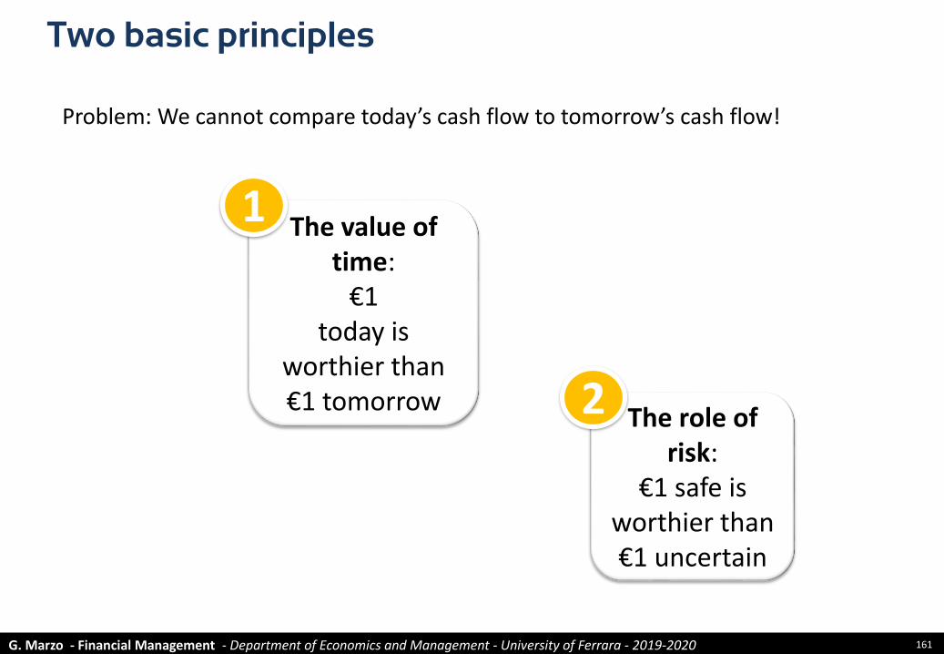
Two basic principles
The value of time:
€1today is
worthier than €1 tomorrow
The role of risk:
€1 safe is worthier than €1 uncertain
1
2
Problem: We cannot compare today’s cash flow to tomorrow’s cash flow!
G. Marzo - Financial Management - Department of Economics and Management - University of Ferrara - 2019-2020 162
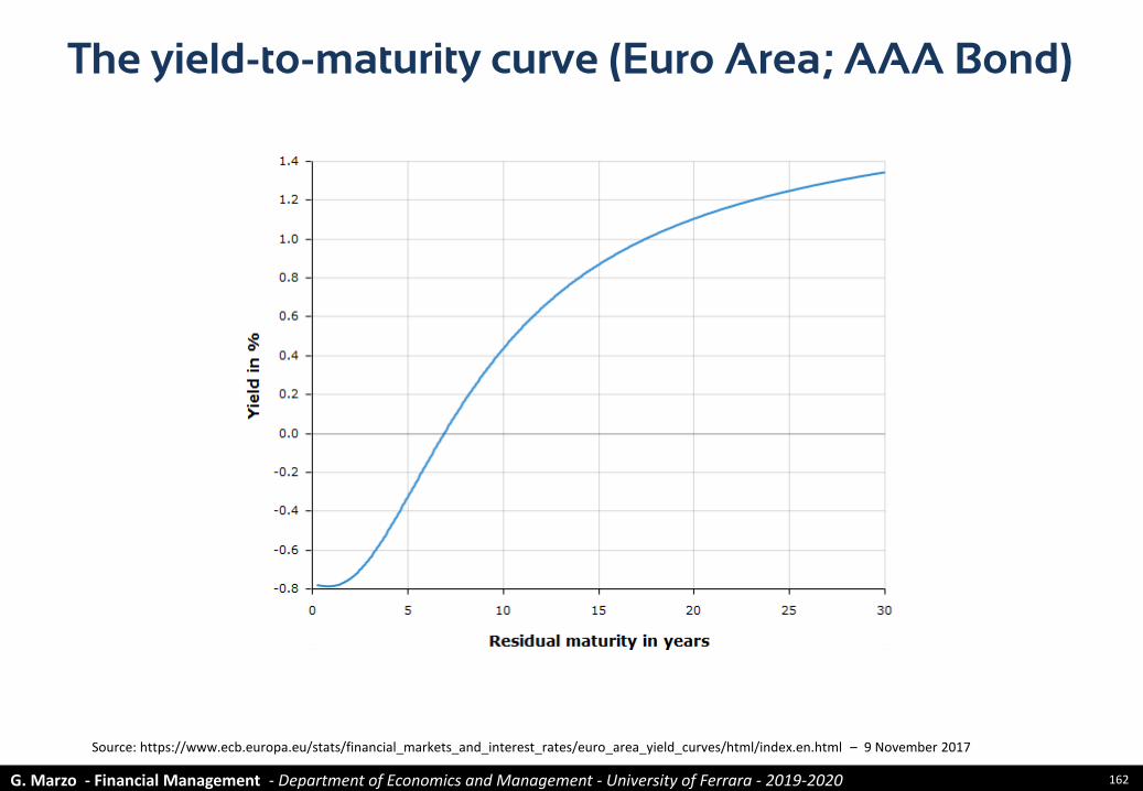
The yield-to-maturity curve (Euro Area; AAA Bond)
Source: https://www.ecb.europa.eu/stats/financial_markets_and_interest_rates/euro_area_yield_curves/html/index.en.html – 9 November 2017
G. Marzo - Financial Management - Department of Economics and Management - University of Ferrara - 2019-2020 163
However the incomparability of today’s to tomorrow’s cash flow is not always taken into consideration
We have in fact two groups of methodology for investment project valuation, depending on the way they deal with that point
Different methodologies

G. Marzo - Financial Management - Department of Economics and Management - University of Ferrara - 2019-2020 164
Graham – Harvey (2002), How Do CFOs Make Capital Budgeting and Capital
Structure Decisions?, Journal of Applied Corporate Finance
G. Marzo - Financial Management - Department of Economics and Management - University of Ferrara - 2019-2020 165
Techniques for valuing
and selecting investment
projects
Investment Projects Appraisal

G. Marzo - Financial Management - Department of Economics and Management - University of Ferrara - 2019-2020 166
Methodologies that DO NOT TAKE into account time value and risk
Accounting Rate of Return
Pay-back period
Methodologies that TAKE into account time value and risk
Discounted Pay-back period
Profitability index
Net Present Value
Internal Rate of Return
Techniques for investment project valuation

G. Marzo - Financial Management - Department of Economics and Management - University of Ferrara - 2019-2020 167
Accounting Rate of Return
P&L 0 1 2 3
Sales 700 820 600
(Monetary Costs) (300) (450) (200)
(Amortisation &Depreciation) (300) (300) (300)
= Operating Income 100 70 100
Balance Sheet 0 1 2 3
Investment Cost 900 900 900 900
(Amortisation) (300) (600) (900)
= Investment Carrying Amount 600 300 0
ROI 0 1 2 3 average
ROI (beginning of year) 11.1% 11.6% 33.3% 18.6%
ROI (average) 13.3% 15.5% 46.6% 25.1%
ROI (end of year) 16.7% 23.3% n.a. ?

G. Marzo - Financial Management - Department of Economics and Management - University of Ferrara - 2019-2020 168
+10
-50
+10+20
+30
+10
time
€
t0
t2 t3 t4
+20
+30
-50
+10+20
+30
+10
time
€
t2 t3 t4
t0
+9.1
+16.5
+22.5
+6.8
Pay-back Period (simple and discounted)
Pay-back Period < 3 years Discounted Pay-back Period (10%) 3 years

G. Marzo - Financial Management - Department of Economics and Management - University of Ferrara - 2019-2020 169
Net Present Value: introduction
-50
+10+20
+30
+10
tempo
€
t1 t2 t3 t4
10/(1.10)1
20/(1.10)2
30/(1.10)3
10/(1.10)4
t0
9,1
16.5
22.5
6.8
55
+55
-50
NPV = +5
N
tt
t
k
FNPV
0 1
G. Marzo - Financial Management - Department of Economics and Management - University of Ferrara - 2019-2020 170
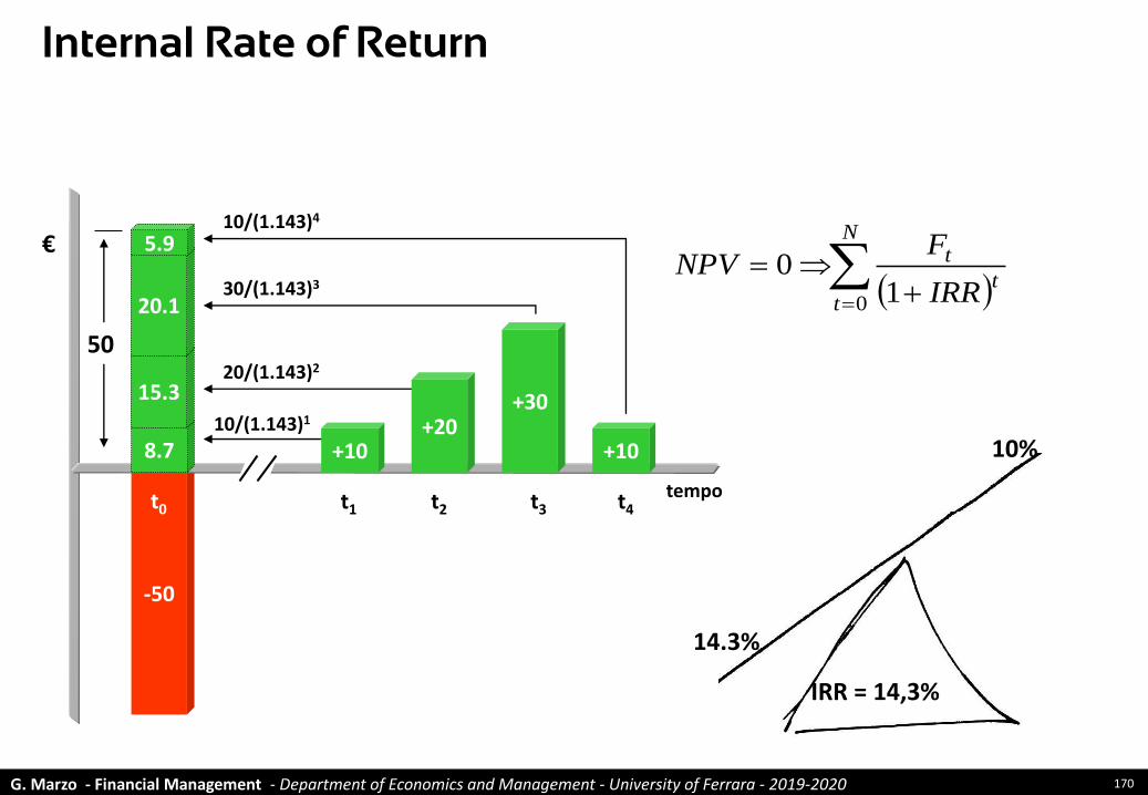
Internal Rate of Return
N
tt
t
IRR
FNPV
0 10
-50
+10+20
+30
+10
tempo
€
t1 t2 t3 t4
10/(1.143)1
20/(1.143)2
30/(1.143)3
10/(1.143)4
t0
8.7
15.3
20.1
5.9
50
14.3%
10%
IRR = 14,3%
G. Marzo - Financial Management - Department of Economics and Management - University of Ferrara - 2019-2020 171
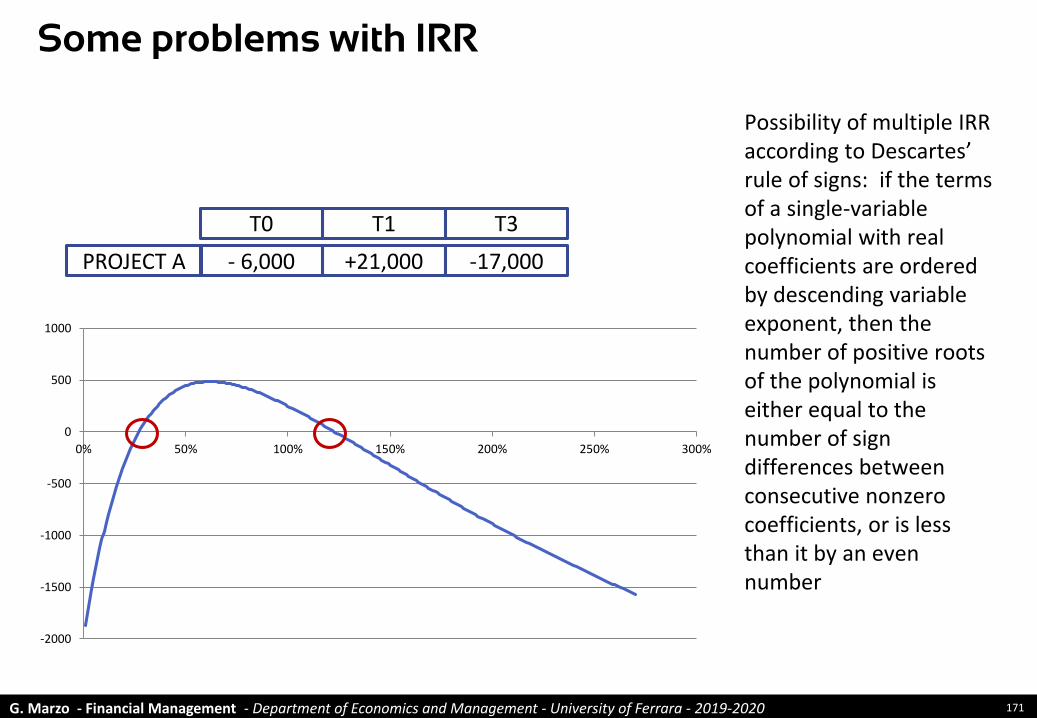
Some problems with IRR
Possibility of multiple IRR according to Descartes’ rule of signs: if the terms of a single-variable polynomial with real coefficients are ordered by descending variable exponent, then the number of positive roots of the polynomial is either equal to the number of sign differences between consecutive nonzero coefficients, or is less than it by an even number
T0 T1
PROJECT A - 6,000 +21,000
T3
-17,000
-2000
-1500
-1000
-500
0
500
1000
0% 50% 100% 150% 200% 250% 300%

G. Marzo - Financial Management - Department of Economics and Management - University of Ferrara - 2019-2020 172
Some problems with IRR
Funding and investment projects could have the same IRR, but when we borrow money we we want a low rate of return, when we lend (or invest) money we want a high rate of return.
T0 T1
PROJECT A - 1,300 +1,690
PROJECT B +1,300 -1,690
IRR NPV (10%)
30% +169.6
30% - 169.6
G. Marzo - Financial Management - Department of Economics and Management - University of Ferrara - 2019-2020 173
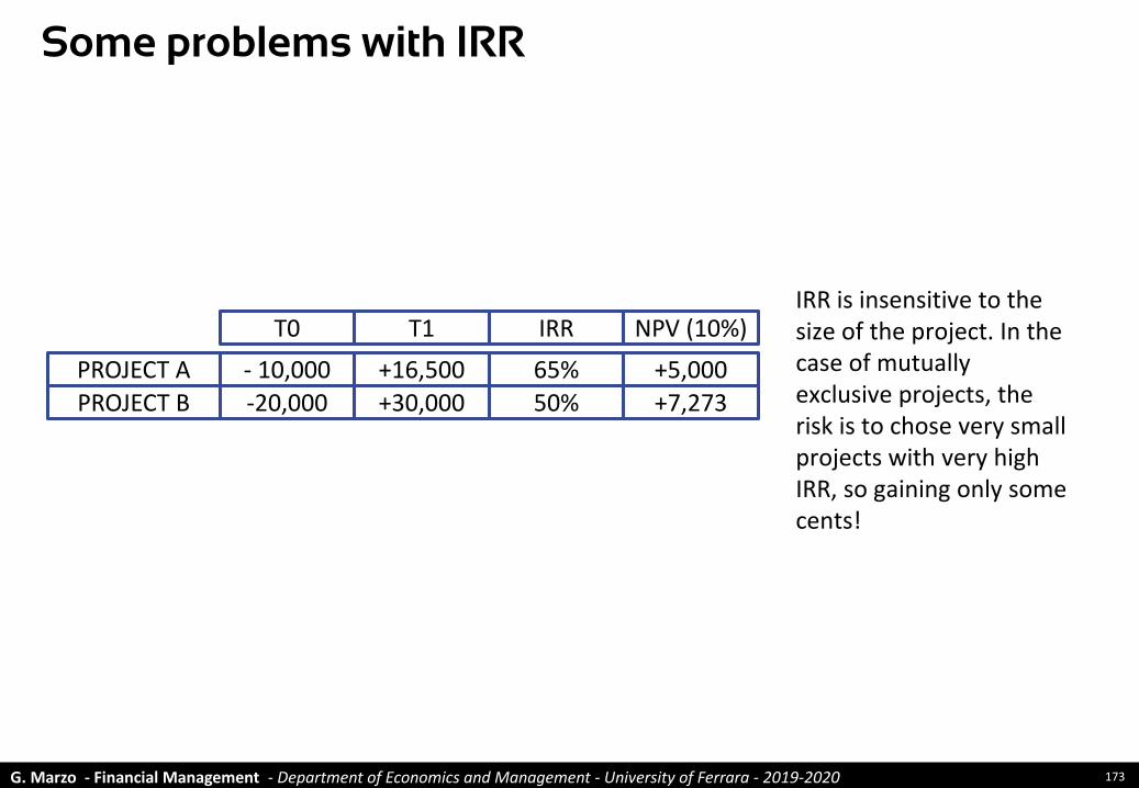
Some problems with IRR
IRR is insensitive to the size of the project. In the case of mutually exclusive projects, the risk is to chose very small projects with very high IRR, so gaining only some cents!
T0 T1
PROJECT A - 10,000 +16,500
PROJECT B -20,000 +30,000
IRR NPV (10%)
65% +5,000
50% +7,273

G. Marzo - Financial Management - Department of Economics and Management - University of Ferrara - 2019-2020 174
Some problems with IRR
Compounded interests: gains from investments that result from earning returns on previously earned returns are calculated at the IRR. If the project under valuation is very profitable, this appears as far from reality!
T0 T1 T2
100 100 100
10 10
10
1IRR = 10%

G. Marzo - Financial Management - Department of Economics and Management - University of Ferrara - 2019-2020 175
Some problems with IRR
𝑁𝑃𝑉 =𝐹0
1+𝑘00 +
𝐹1
1+𝑘11+
𝐹2
1+𝑘22+
𝐹3
1+𝑘33+…
𝐼𝑅𝑅:𝐹0
1+𝐼𝑅𝑅 0 +𝐹1
1+𝐼𝑅𝑅 1+𝐹2
1+𝐼𝑅𝑅 2+𝐹3
1+𝐼𝑅𝑅 3+…
One rate fits all!
With NPV different discount rates can be used for discounting cash flows expected in different periods.When using IRR all cash flows are discounted at the same rate (the IRR).
G. Marzo - Financial Management - Department of Economics and Management - University of Ferrara - 2019-2020 176
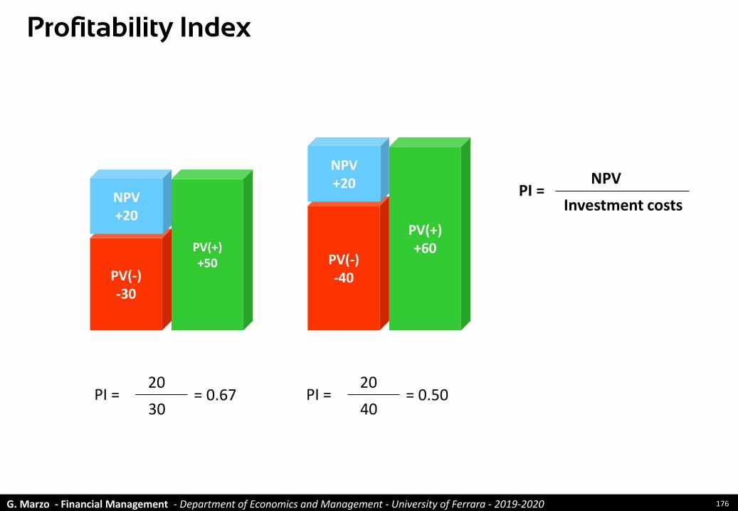
Profitability Index
PV(+)+50
PV(+)+60
PV(-)-40PV(-)
-30
NPV+20
NPV+20
PI = 20
30= 0.67 PI =
20
40= 0.50
PI = NPV
Investment costs

G. Marzo - Financial Management - Department of Economics and Management - University of Ferrara - 2019-2020 177
Techniques for valuing
and selecting investment
projects- The NPV: The expected cash
flow -
Investment Projects Appraisal

G. Marzo - Financial Management - Department of Economics and Management - University of Ferrara - 2019-2020 178
Only incremental cash flows are important
Consider operating cash flow (net of taxes on operating income) and capital expenses
Be careful about the role of taxes
Do not confuse average vs incremental profits
Consider the effect of Net Working Capital on cash flow
Forget sunk costs
Remember opportunity costs
Neglect allocated overhead costs
Remember salvage value
Consider incidental effects
Be careful when considering inflation
How to calculate cash flow for NPV

G. Marzo - Financial Management - Department of Economics and Management - University of Ferrara - 2019-2020 179
Net operating cash flow: Calculation
INCOME STATEMENT
Sales 800
(Operating Costs) (300)
EBITDA 500
(Amortisation and provisions) (200)
Operating Profit or EBIT 300
(Taxes on Operating Income) (100)
Net Operating Profit After Taxes (NOPAT) 200
CASH FLOW
NOPAT 200
+ Amortisation and provisions 200
±D Net Working Capital (150)
Unlevered Cash Flow from Operations 250
(Capital Expenses) (600)
Divestments 50
Unlevered Free Cash Flow to the firm (300)
CAPITAL EMPLOYED
±D Net Working Capital (150)
(Capital Expenses) (600)
Divestments 50
Net Capital Employed (700)
We already know that! We can calculate Taxes on Operating Income by simply multiplying EBIT by the Tax rate.
Please, remember that Net Working Capital is an investment and as such a reduction in cash flow.

G. Marzo - Financial Management - Department of Economics and Management - University of Ferrara - 2019-2020 180
Division A is losing money, but the opportunity for a new project with a positive NPV arises.What to do?
Accept the project
Refuse the project
Do not confuse average vs incremental profits

G. Marzo - Financial Management - Department of Economics and Management - University of Ferrara - 2019-2020 181
Sunk costs
Firm A has already invested € 200 in an R&D project for launching a new product.
Manufacturing and marketing the product require a further investment of €100.
Expected net cash flows from this new investment have a present value of € 130.
What to do?
Accept the project
Refuse the project

G. Marzo - Financial Management - Department of Economics and Management - University of Ferrara - 2019-2020 182
Opportunity costs
Firm B owns a machinery that has a market price of € 30 on the secondary market.
The firm is analysing a project requiring an investment of €100 together with the machinery.
Expected cash flows from this new investment have a present value of € 120.
What to do?
Accept the project
Refuse the project

G. Marzo - Financial Management - Department of Economics and Management - University of Ferrara - 2019-2020 183
The opportunity cost of being a mom
JobAverage hours
per weekPayroll
Child care 7 € 230.40
Washing and ironing 4 € 155.40
Chauffeur 4 € 208.00
Personal shopper 1 € 150.00
Colf 14 € 560.00
Chef 10.5 € 1,260.00
Tutor 6 € 480.00
Total 46.5 € 3,045.00
Source: La Repubblica, Il "lavoro di mamma" varrebbe oltre 3mila euro netti al mese, se fosse pagato,http://www.repubblica.it/economia/miojob/2017/05/11/news/mamma_lavoro-165156145/

G. Marzo - Financial Management - Department of Economics and Management - University of Ferrara - 2019-2020 184
Overhead costs
Firm C is valuing a new project, which has a cost of €100. Expected net cash flows from this new investment have a present value of € 125.
Once run, the new project will be charged for € 30 as its share of overhead costs. The accounting system of the firm, in fact, allocates a share of overhead costs to all projects of the firm.
What to do?
Accept the project
Refuse the project

G. Marzo - Financial Management - Department of Economics and Management - University of Ferrara - 2019-2020 185
The role of taxes
Tax rules can strongly modify the NPV of a project. For instance: Italian rules are now giving the possibility to deduct a cost larger than actual,
in some specific cases (super-ammortamento)
The deferral of taxes increases the NPV of a project
The impact of tax rules must be carefully taken into account when calculating NPV.
My suggestion is to first calculate the NPV of the project without tax benefits, and then the same NPV but considering tax benefits.
The risk is in fact that a firm could decide to undertake a project due to the fiscal benefits relating to it.
G. Marzo - Financial Management - Department of Economics and Management - University of Ferrara - 2019-2020 186
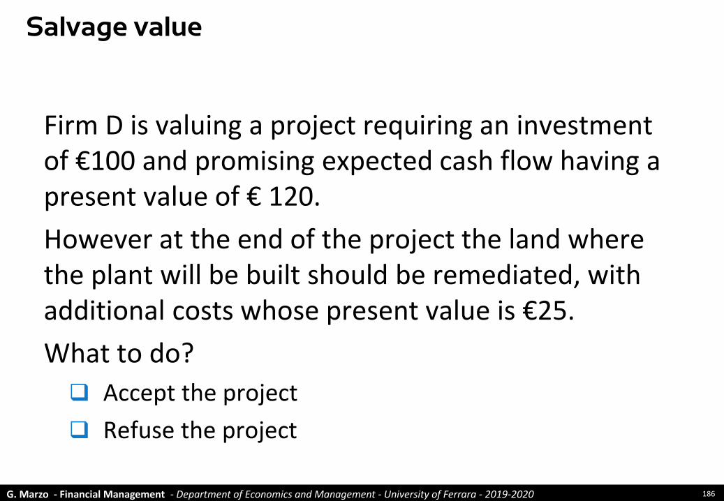
Firm D is valuing a project requiring an investment of €100 and promising expected cash flow having a present value of € 120.
However at the end of the project the land where the plant will be built should be remediated, with additional costs whose present value is €25.
What to do?
Accept the project
Refuse the project
Salvage value

G. Marzo - Financial Management - Department of Economics and Management - University of Ferrara - 2019-2020 187
Incidental effects of a project
A new product or service can cut sales of existing products or services
Sometimes the are important network effects: the new project can increase the value of older projects
The new project could increase the risk of the firm since it needs a large amount of funds

G. Marzo - Financial Management - Department of Economics and Management - University of Ferrara - 2019-2020 188
Inflation
It appears that it is only necessary to be
consistent: working with both cash flows and
discount rate expressed in real or inflated terms
1
In practice it is better to incorporate inflation in cost and
revenues values.Cash flows are in fact delayed with respect to revenues and
costs and therefore the cash flow of a specific year is influenced by inflation rates of many previous
years
2

G. Marzo - Financial Management - Department of Economics and Management - University of Ferrara - 2019-2020 189
Only incremental cash flows are important
Consider operating cash flow (net of taxes on operating income) and capital expenses
Be careful about the role of taxes
Do not confuse average vs incremental profits
Consider the effect of Net Working Capital on cash flow
Forget sunk costs
Remember opportunity costs
Neglect allocated overhead costs
Remember salvage value
Consider incidental effects
Be careful when considering inflation
Wrap-up: How to calculate cash flow for NPV

G. Marzo - Financial Management - Department of Economics and Management - University of Ferrara - 2019-2020 190
Techniques for valuing
and selecting investment
projects- The NPV: Weighted Average
Cost of Capital -
Investment Projects Appraisal
G. Marzo - Financial Management - Department of Economics and Management - University of Ferrara - 2019-2020 191
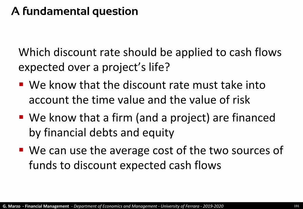
Which discount rate should be applied to cash flows expected over a project’s life?
We know that the discount rate must take into account the time value and the value of risk
We know that a firm (and a project) are financed by financial debts and equity
We can use the average cost of the two sources of funds to discount expected cash flows
A fundamental question
G. Marzo - Financial Management - Department of Economics and Management - University of Ferrara - 2019-2020 192
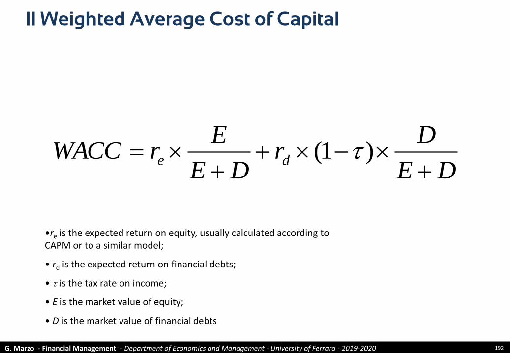
Il Weighted Average Cost of Capital
DE
Dr
DE
ErWACC de
)1(
•re is the expected return on equity, usually calculated according to CAPM or to a similar model;
• rd is the expected return on financial debts;
• is the tax rate on income;
• E is the market value of equity;
• D is the market value of financial debts

G. Marzo - Financial Management - Department of Economics and Management - University of Ferrara - 2019-2020 193
How to determine the minimum acceptable return (MAR) a shareholder would ask for investing in a firm?
A problem..
G. Marzo - Financial Management - Department of Economics and Management - University of Ferrara - 2019-2020 194
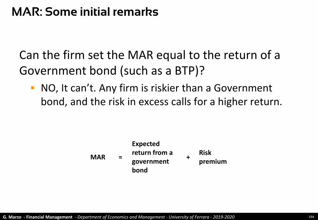
Can the firm set the MAR equal to the return of a Government bond (such as a BTP)?
NO, It can’t. Any firm is riskier than a Government bond, and the risk in excess calls for a higher return.
MAR: Some initial remarks
MAR =
Expected return from a government bond
+Risk premium

G. Marzo - Financial Management - Department of Economics and Management - University of Ferrara - 2019-2020 195
Can the firm set the MAR equal to the cost of its financial position?
NO, It can’t. Shareholders bear a higher risk than banks, since banks have priority over shareholders as for remuneration and the reimbursement of capital. MAR is therefore expected to be higher than the cost of financial debt.
MAR: Some initial remarks

G. Marzo - Financial Management - Department of Economics and Management - University of Ferrara - 2019-2020 196
If the firm finances an investment project by using new and additional bank loans, can it set the MAR equal to the cost of this new debt?
NO, It can’t. Fund providers finance the whole firm, not specific projects, and the return they ask depends on the risk of the whole firm
The additional debt also increases the risk of the firm, other remaining the same
MAR: Some initial remarks

G. Marzo - Financial Management - Department of Economics and Management - University of Ferrara - 2019-2020 197
As for the return of a Government bond, which bond should the firm select?
It depends on the investment horizon.
MAR: Some initial remarks
Source: http://www.rendimentibtp.it - 10 November 2017
-1,00%
-0,50%
0,00%
0,50%
1,00%
1,50%
2,00%
2,50%
3,00%
3,50%
0 10 20 30 40 50 60
Net Return
in the long run net return is between 2.7% and 3%

G. Marzo - Financial Management - Department of Economics and Management - University of Ferrara - 2019-2020 198
Which are the main determinants of the risk premium of a firm?
They are the industry the firm operates in (and the way it do it) and the financing decision of the firm
In other words: Business Risk and Financial Risk
MAR: Some initial remarks

G. Marzo - Financial Management - Department of Economics and Management - University of Ferrara - 2019-2020 199
How can the firm calculate its MAR?
For listed firms, there are models that can be implemented on market data (e.g. CAPM)
For non-listed firms, we can use multiple sources of data (market-based risk premia referring to industry, competitors, book values, etc.)
MAR: Some initial remarks

G. Marzo - Financial Management - Department of Economics and Management - University of Ferrara - 2019-2020 200
b
The CAPM at a glance
Expected return on
equity=
Risk-free rate(return from
securities with no risk)
Risk-premium for the equity investment
+
Business risk
Financial risk
Firm-related, and
therefore diversifiable,
risk
Undiversifiablerisk
Market risk-premium
Risk-free rate
Expected return from
market
From 4% to 6.5% on historical basis
The return form government
bond, such as high maturity BTP
Calculated through
econometric models

G. Marzo - Financial Management - Department of Economics and Management - University of Ferrara - 2019-2020 201
The Beta: A graphical representation
The Beta measures the association between the expected return of an asset (e.g. a stock) and the expected return of the entire market
time
Ris
k p
rem
ium
%
Market
b > 1
b < 1
time
Market
b < 0Ris
k p
rem
ium
%

G. Marzo - Financial Management - Department of Economics and Management - University of Ferrara - 2019-2020 202
Beta is the risk that remains after a fully
diversification
Diversifiable risk, also known as company-specific or unsystematic risk, can be cancelled away through diversification
Market risk, also known as non-diversifiable or systematic risk is the risk that remains after diversification.
Non-diversifiable risk
0
66
132
198
264
330
396
461
527
593
659
725
1 2 3 4 5 6 7 8 9 10 11 12 13 14 15 16 17 18 19 20
Variance of the portfolio
No. of stocks in portfolio

G. Marzo - Financial Management - Department of Economics and Management - University of Ferrara - 2019-2020 203
Biotech (NYSE)
bOXIGEN = 1.92
bDECODE GENETICS = 1.32
0
2000
4000
6000
8000
10000
12000
14000
Nov-94 Mar-96 Jul-97 Dec-98 Apr-00 Sep-01 Jan-03
0
5
10
15
20
25
30
35
40
DowJones OXIGEN DECODE GENETICS

G. Marzo - Financial Management - Department of Economics and Management - University of Ferrara - 2019-2020 204
Utilities (NYSE)
bAEP = 0.06
0
2000
4000
6000
8000
10000
12000
14000
Nov-94 Mar-96 Jul-97 Dec-98 Apr-00 Sep-01 Jan-03
0
5
10
15
20
25
30
35
40
45
50
DowJones American Electric Power

G. Marzo - Financial Management - Department of Economics and Management - University of Ferrara - 2019-2020 205
The Energy industry (NYSE)
Source: Yahoo!Finance end of 2002
blevered (Weighted average) = 0.48
Company Beta Price/Book Leverage
Exxon Mobil Corporation (XOM) 0.33 3.22 0.15
BP plc (BP) 0.59 2.22 0.33
TOTAL Fina Elf S.A. (TOT) 0.60 2.79 0.44
Royal Dutch Petroleum Com (RD) 0.76 2.50 0.31
ChevronTexaco Corporation (CVX) n.d. 2.30 0.51
Shell Transport & Trading (SC) 0.77 2.54 0.31
Eni S.p.A. (E) 0.37 2.40 0.47
PetroChina Company Limite (PTR) 0.21 0.97 0.28
ConocoPhillips (COP) 0.66 1.13 0.68
Schlumberger Ltd. (SLB) 0.99 2.79 0.86

G. Marzo - Financial Management - Department of Economics and Management - University of Ferrara - 2019-2020 206
Beta and the Capital structure
Usually, beta and leverage (Debt-to-Equity ratio) are positively associated
0
0.2
0.4
0.6
0.8
1
1.2
0 0.1 0.2 0.3 0.4 0.5 0.6 0.7 0.8 0.9 1
XOM
PTR
E
COP
SLB
BP
RD
SC
TOT
b
leverage
G. Marzo - Financial Management - Department of Economics and Management - University of Ferrara - 2019-2020 207
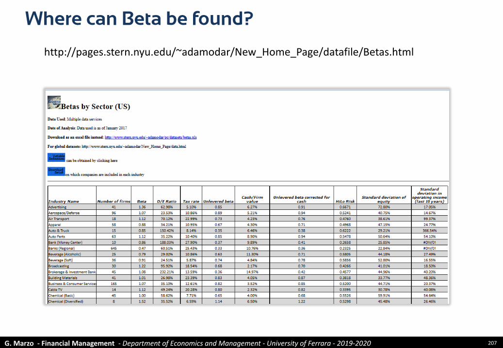
Where can Beta be found?
http://pages.stern.nyu.edu/~adamodar/New_Home_Page/datafile/Betas.html

G. Marzo - Financial Management - Department of Economics and Management - University of Ferrara - 2019-2020 208
Calculating the WACC for Eni Group
Risk-free rate(30y BTP at the end of 2002*)
5.3%
Market RiskPremium
(historical mean)6.0%
Tax rate35.0%
Costs onNet Financial Position***
5.4%
Equity Opportunity costke= 8.84%
b levered0,59
Costs on NFP After taxeskd(1-t)= 3.51%
WACC=7.5% - 8.8%
* Source: BankItalia** Market capitalisation (end of 2002 – beginning of 2003) 62 billion
Average Equity Book Value (2001 - 2002) 29 billionAvaerage Net Financial Position (2001 – 2002) 10 billion
*** Equal to the risk-free rate
Leverage** (D/E)
E/(D+E)
Book values Market values
O.33 0
O.75 1
O.25 0D/(D+E)

G. Marzo - Financial Management - Department of Economics and Management - University of Ferrara - 2019-2020 209
Equity opportunity cost for a SME
Focus: Direct competitors Focus: Capital Markets
Database AIDA
Focus on industry (ATECO code)
Focus on direct competitors
Calculation of average ROE (over the last 3 to 5
years)
Minimum acceptable ROE
Focus on industry
Calculation of the market risk premium for all the
companies of the industry
Calculation of the
average market risk
premium
Sum of the BTP return and the average market risk
premium
= 16,5% = 14,5% Minimum acceptable return

G. Marzo - Financial Management - Department of Economics and Management - University of Ferrara - 2019-2020 210
The build-up approach to beta
•Economic, social and political environment
•Market structure•Competitive position of the firm
Net earnings
EBITSales
less:•variable costs•Fixed costs
less:• interests expenses• taxes expenses
Business risk Financial risk
Operating riskEconomic risk
Source: Hawawini G.and– Viallet C., Finance for Executives, South-Western College, Cincinnati, Ohio, 1999
𝛽𝑒𝑞𝑢𝑖𝑡𝑦 = 𝛽𝑎𝑠𝑠𝑒𝑡𝑠 + 𝛽𝑎𝑠𝑠𝑒𝑡𝑠 − 𝛽𝑑𝑒𝑏𝑡 × 1 − 𝜏 ×𝐷
𝐸and with 𝛽𝑑𝑒𝑏𝑡=0
𝛽𝑒𝑞𝑢𝑖𝑡𝑦 = 𝛽𝑎𝑠𝑠𝑒𝑡𝑠 1 + 1 − 𝜏 ×𝐷
𝐸
𝛽𝑒𝑞𝑢𝑖𝑡𝑦 is also know as 𝛽𝑙𝑒𝑣𝑒𝑟𝑒𝑑𝛽𝑎𝑠𝑠𝑒𝑡𝑠 is also know as 𝛽𝑢𝑛𝑙𝑒𝑣𝑒𝑟𝑒𝑑
𝛽𝑎𝑠𝑠𝑒𝑡𝑠 = 𝛽𝑠𝑎𝑙𝑒𝑠 1 +𝑃𝑉𝐹𝑖𝑥𝑒𝑑 𝑐𝑜𝑠𝑡𝑠
𝑃𝑉𝑉𝑎𝑟𝑖𝑎𝑏𝑙𝑒 𝑐𝑜𝑠𝑡𝑠
𝜏 is the tax rate on income𝐸 is the market value of equity 𝐷 is the market value of debt
G. Marzo - Financial Management - Department of Economics and Management - University of Ferrara - 2019-2020 211
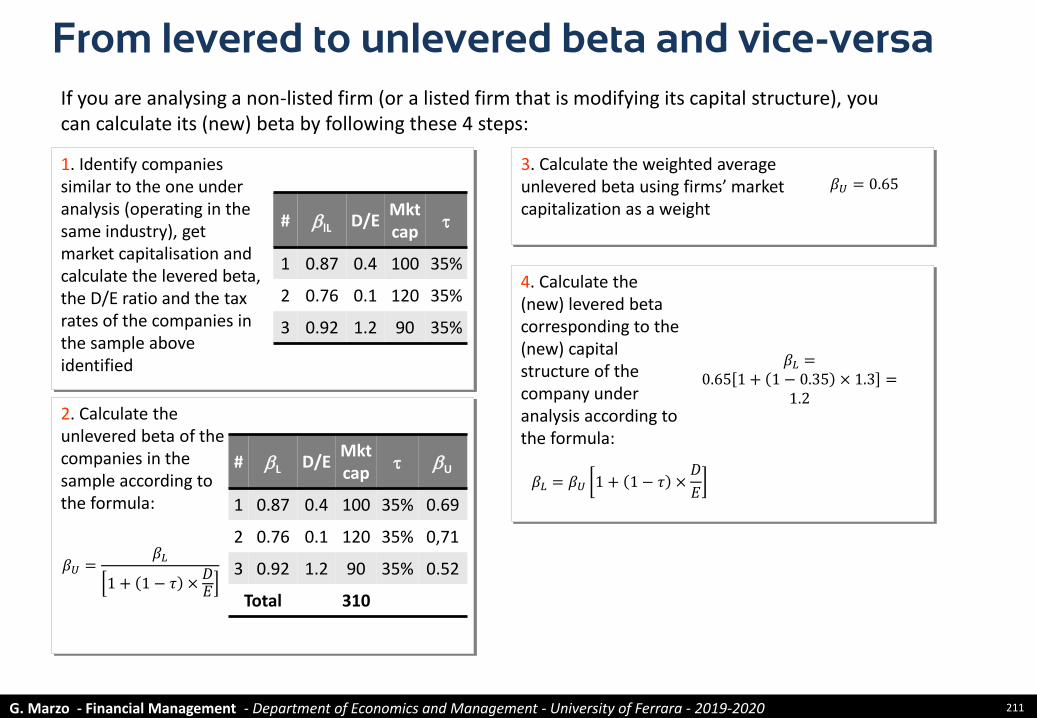
From levered to unlevered beta and vice-versa
1. Identify companies similar to the one under analysis (operating in the same industry), get market capitalisation and calculate the levered beta, the D/E ratio and the tax rates of the companies in the sample above identified
3. Calculate the weighted average unlevered beta using firms’ market capitalization as a weight
If you are analysing a non-listed firm (or a listed firm that is modifying its capital structure), you can calculate its (new) beta by following these 4 steps:
# blL D/EMktcap
1 0.87 0.4 100 35%
2 0.76 0.1 120 35%
3 0.92 1.2 90 35%
2. Calculate the unlevered beta of the companies in the sample according to the formula:
𝛽𝑈 =𝛽𝐿
1 + 1 − 𝜏 ×𝐷𝐸
# bL D/EMktcap
bU
1 0.87 0.4 100 35% 0.69
2 0.76 0.1 120 35% 0,71
3 0.92 1.2 90 35% 0.52
Total 310
𝛽𝑈 = 0.65
4. Calculate the (new) levered beta corresponding to the (new) capital structure of the company under analysis according to the formula:
𝛽𝐿 = 𝛽𝑈 1 + 1 − 𝜏 ×𝐷
𝐸
𝛽𝐿 =0.65 1 + 1 − 0.35 × 1.3 =
1.2

G. Marzo - Financial Management - Department of Economics and Management - University of Ferrara - 2019-2020 212
Risk analysisInvestment Projects Appraisal
G. Marzo - Financial Management - Department of Economics and Management - University of Ferrara - 2019-2020 213
Risk is usually ignored in investment project valuation
Why
People is more focussed on return
They are not used to assess risk
They don’t know how to take risk into account
Risk analysis in investment projects

G. Marzo - Financial Management - Department of Economics and Management - University of Ferrara - 2019-2020 214
Project risk analysis
Pay-Back Period
1
Sensitivity Analysis
2
Real Option thinking
4
Montecarlosimulation
3
G. Marzo - Financial Management - Department of Economics and Management - University of Ferrara - 2019-2020 215
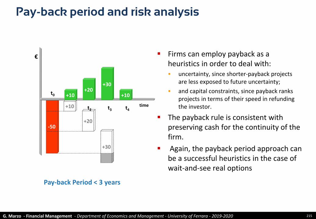
Pay-back period and risk analysis
Firms can employ payback as a heuristics in order to deal with: uncertainty, since shorter-payback projects
are less exposed to future uncertainty;
and capital constraints, since payback ranks projects in terms of their speed in refunding the investor.
The payback rule is consistent with preserving cash for the continuity of the firm.
Again, the payback period approach can be a successful heuristics in the case of wait-and-see real options
+10
-50
+10+20
+30
+10
time
€
t0
t2 t3 t4
+20
+30
Pay-back Period < 3 years
G. Marzo - Financial Management - Department of Economics and Management - University of Ferrara - 2019-2020 216
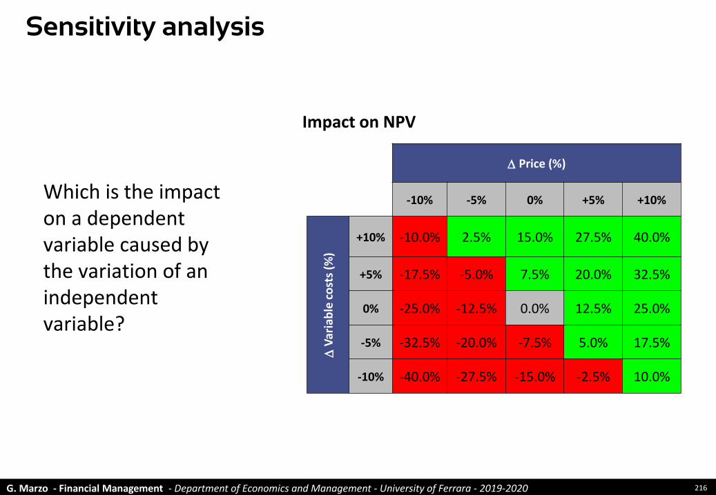
Which is the impact on a dependent variable caused by the variation of an independent variable?
Sensitivity analysis
D Price (%)
-10% -5% 0% +5% +10%
D V
aria
ble
cost
s(%
)
+10% -10.0% 2.5% 15.0% 27.5% 40.0%
+5% -17.5% -5.0% 7.5% 20.0% 32.5%
0% -25.0% -12.5% 0.0% 12.5% 25.0%
-5% -32.5% -20.0% -7.5% 5.0% 17.5%
-10% -40.0% -27.5% -15.0% -2.5% 10.0%
Impact on NPV
G. Marzo - Financial Management - Department of Economics and Management - University of Ferrara - 2019-2020 217
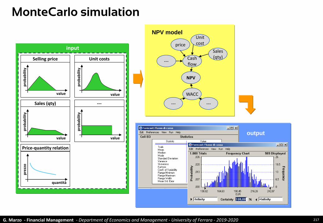
MonteCarlo simulationp
rob
abili
ty
value
Selling price
pro
bab
ility
value
Sales (qty)
pro
bab
ility
value
Unit costs
pro
bab
ility
value
---
pre
zzo
quantità
Price-quantity relation
input
output
NPV modelUnit costprice
Sales (qty)
NPV
WACC
--- ---
Cash flow
---

G. Marzo - Financial Management - Department of Economics and Management - University of Ferrara - 2019-2020 218
A real case
Trials 1,000Mean 33.19Median 38.20

G. Marzo - Financial Management - Department of Economics and Management - University of Ferrara - 2019-2020 219
A software for Montecarlo simulation
http://www.oracle.com/us/products/applications/crystalball/overview/index.html

G. Marzo - Financial Management - Department of Economics and Management - University of Ferrara - 2019-2020 220
Introducing investment
projects techniques in
SMEs
Investment Projects Appraisal

G. Marzo - Financial Management - Department of Economics and Management - University of Ferrara - 2019-2020 221
Capital Budgeting techniques
Ownership Sales
Capital Budgeting techniques Family Other<€10 mln
€10-20 mln
€20-43 mln
TOT
Costs-Benefits analysis 22.2% 8.1% 21.7% 11.2% 16.8% 15.6%
Accounting ratios 20.5% 7.5% 13.3% 10.4% 18.0% 14.5%
NPV 6.5% 21.1% 18.3% 19.2% 6.8% 13.3%
Hurdle rates 13.0% 13.0% 11.7% 11.2% 14.9% 13.0%
Payback period 8.1% 15.5% 10.0% 15.2% 9.3% 11.6%
Sensitivity analysis 13.5% 5.0% 1.7% 5.6% 15.5% 9.5%
Discounted Payback period 4.3% 13.7% 6.7% 14.4% 5.0% 8.7%
Profitability index 6.5% 2.5% 11.7% 4.8% 1.9% 4.6%
Scenario analysis 2.7% 6.2% 0.0% 2.4% 7.5% 4.3%
Adjusted NPV 1.6% 4.3% 3.3% 2.4% 3.1% 2.9%
Real options 0.5% 3.1% 1.7% 3.2% 0.6% 1.7%
IRR 0.5% 0.0% 0.0% 0.0% 0.6% 0.3%
Source: Marzo. Scarpino e Cappello, Le PMI italiane e la valutazione economica dei progetti di investimento, Amministrazione & Finanza n. 4/2016

G. Marzo - Financial Management - Department of Economics and Management - University of Ferrara - 2019-2020 222
The cost of capital
Family business (Sales) Others (Sales)
The cost of capital<€10 mln
€10-20 mln
€20-43 mln
TOT<€10 mln
€10-20 mln
€20-43 mln
TOT
Not estimated 33.3% 26.9% 29.3% 32.4% 30.0% 28.0% 52.0% 38.3%
Average of past returns (e.g. Return On Equity) 19.0% 26.9% 20.0% 21.4% 50.0% 12.0% 20.0% 21.7%Regulatory decisions 0.0% 7.7% 5.3% 6.6% 0.0% 16.0% 8.0% 10.0%
Return expected by funds providers 0.0% 0.0% 1.3% 0.5% 0.0% 0.0% 0.0% 0.0%
Capital Asset Pricing Model 42.9% 30.8% 34.7% 30.2% 10.0% 28.0% 16.0% 20.0%Other 4.8% 7.7% 9.3% 8.8% 10.0% 16.0% 4.0% 10.0%TOT 100.0% 100.0% 100.0% 100.0% 100.0% 100.0% 100.0% 100.0%
Source: Marzo. Scarpino e Cappello, Le PMI italiane e la valutazione economica dei progetti di investimento, Amministrazione & Finanza n. 4/2016