introduction to water assessment in gabi software · introduction to water assessment in gabi...

Introduction to Water Assessment in GaBi Software

Version 2.0 - January 2017

Authors

Daniel Thylmann [email protected]

Dr. Thilo Kupfer [email protected]

mailto:[email protected]

0

List of Contents

1 Introduction ................................................................................................................. 2

2 Terminology ................................................................................................................ 3

2.1 Consumptive and degradative use ................................................................................... 3

2.2 Water scarcity footprint ......................................................................................................... 4

3 Water flows in GaBi Software ................................................................................ 7

3.1 Input flows ................................................................................................................................ 7

3.2 Output flows ............................................................................................................................. 8

3.3 Additional water flows in GaBi.......................................................................................... 10

3.4 Renaming of flows in SP32 ............................................................................................... 10

4 Regionalization ........................................................................................................ 11

4.1 Regionalized flows in GaBi ............................................................................................... 11

4.2 Use of regionalized flows in GaBi datasets.................................................................. 12

5 Impact Assessment – Water quantities in GaBi............................................. 14

5.1 Water use ............................................................................................................................... 14

5.2 Water consumption .............................................................................................................. 14

5.3 Water scarcity footprint (WSI, AWaRe, UBP) ............................................................. 15

6 Limitations ................................................................................................................. 17

7 Literature .................................................................................................................... 19

List of Figures

Figure 1: Water use and water consumption ................................................................................... 4

Figure 2: From water use to water scarcity footprint ....................................................................... 5

Figure 3-1: Structure of water input flows in GaBi Software ............................................... 7

Figure 3-2: Structure of water output flows in GaBi Software ............................................ 8


2

1 Introduction

Freshwater scarcity is recognized as one of the most pressing environmental issues today

and in the future. There is an increasing interest in the LCA community to assess water use

from a LCA perspective.

In August 2014, a new standard under the 14000 series (environmental management) has

been released by the ISO (International Organization for Standardization): ISO 14046 on

Water Footprint [ISO 14046]. The standard specifies principles, requirements and guide-

lines related to water footprint assessment of products, processes and organizations based

on life cycle assessment (LCA). A water footprint assessment conducted according to this

international standard:

is based on a life cycle assessment (according to ISO 14044);

is modular (i.e. the water footprint of different life cycle stages can be summed to

represent the water footprint);

identifies potential environmental impacts related to water;

includes relevant geographical and temporal dimensions;

identifies quantity of water use and changes in water quality;

utilizes hydrological knowledge.

With this standard, regional impact assessment is officially introduced into the LCA world.

With SP32, GaBi follows these developments and introduces regionally specific elementary

flows and new quantities as a first step towards a comprehensive assessment of water data.

To make best use of this new implementation, it is important to have a correct understanding

of the principles that are underlying water assessment in the GaBi software. This document

introduces the latest GaBi water assessment terminology and details on how water use and

water consumption can be assessed using GaBi Software.


3

2 Terminology

Water assessment in GaBi follows methods and terminology as defined by the

UNEP/SETAC working group on water and the new ISO standard (Bayart et al. 2010, Pfister

et al. 2009, ISO 14046). According to these publications, the following terms are used:

Water use: use of water by human activity. Use includes, but is not limited to, any water

withdrawal, water release or other human activities within the drainage basin impacting water

flows and quality.

Water consumption: water removed from, but not returned to the same drainage basin. Wa-

ter consumption can be because of evaporation, transpiration, product integration or release

into a different drainage basin or the sea. Evaporation from reservoirs is considered water

consumption.

Groundwater: water which is being held in, and can be recovered from, an underground

formation.

Green water refers to the precipitation on land that does not run off or recharges the ground-

water but is stored in the soil or temporarily stays on top of the soil or vegetation. Eventually,

this part of precipitation evaporates or transpires through plants. Green water can be made

productive for crop growth.

Blue water refers to water withdrawn from ground water or surface water bodies. The blue

water inventory of a process includes all freshwater inputs but excludes rainwater.

Fresh water and sea water: “Fresh water” is defined as water having a low concentration of

dissolved solids (ISO 14046)1. This term specifically excludes sea water and brackish water.

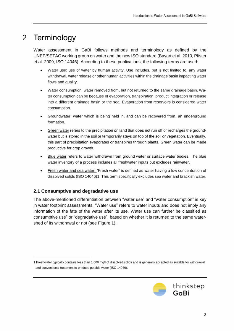
2.1 Consumptive and degradative use

The above-mentioned differentiation between “water use” and “water consumption” is key

in water footprint assessments. “Water use” refers to water inputs and does not imply any

information of the fate of the water after its use. Water use can further be classified as

consumptive use” or “degradative use”, based on whether it is returned to the same water-

shed of its withdrawal or not (see Figure 1).

1 Freshwater typically contains less than 1 000 mg/l of dissolved solids and is generally accepted as suitable for withdrawal

and conventional treatment to produce potable water (ISO 14046).


4

Figure 1: From water use to water scarcity footprint

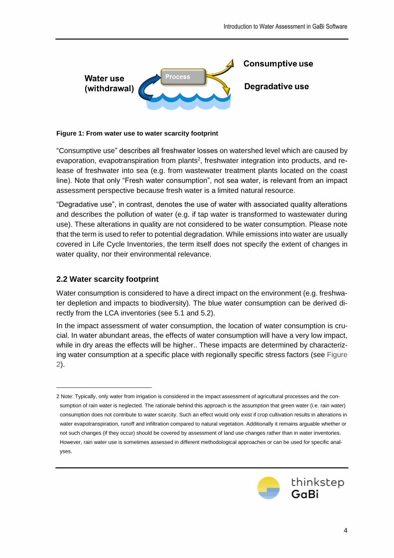
“Consumptive use” describes all freshwater losses on watershed level which are caused by

evaporation, evapotranspiration from plants2, freshwater integration into products, and re-

lease of freshwater into sea (e.g. from wastewater treatment plants located on the coast

line). Note that only “Fresh water consumption”, not sea water, is relevant from an impact

assessment perspective because fresh water is a limited natural resource.

“Degradative use”, in contrast, denotes the use of water with associated quality alterations

and describes the pollution of water (e.g. if tap water is transformed to wastewater during

use). These alterations in quality are not considered to be water consumption. Please note

that the term is used to refer to potential degradation. While emissions into water are usually

covered in Life Cycle Inventories, the term itself does not specify the extent of changes in

water quality, nor their environmental relevance.

2.2 Water scarcity footprint

Water consumption is considered to have a direct impact on the environment (e.g. freshwa-

ter depletion and impacts to biodiversity). The blue water consumption can be derived di-

rectly from the LCA inventories (see 5.1 and 5.2).

In the impact assessment of water consumption, the location of water consumption is cru-

cial. In water abundant areas, the effects of water consumption will have a very low impact,

while in dry areas the effects will be higher.. These impacts are determined by characteriz-

ing water consumption at a specific place with regionally specific stress factors (see Figure

2).

2 Note: Typically, only water from irrigation is considered in the impact assessment of agricultural processes and the con-

sumption of rain water is neglected. The rationale behind this approach is the assumption that green water (i.e. rain water)

consumption does not contribute to water scarcity. Such an effect would only exist if crop cultivation results in alterations in

water evapotranspiration, runoff and infiltration compared to natural vegetation. Additionally it remains arguable whether or

not such changes (if they occur) should be covered by assessment of land use changes rather than in water inventories.

However, rain water use is sometimes assessed in different methodological approaches or can be used for specific anal-

yses.


5

Figure 2: From water use to water scarcity footprint

Different methods to assess water scarcity are published (for a recent review see SALA ET.

AL 2016 ). The following methods are implemented into the GaBi software (please refer to

the respective publications for a description of how the characterization factors are calcu-

lated):

Pfister et al. developed the water stress index (WSI) (PFISTER ET AL.

2009). Because of its robust documentation and easy access to the characterization

factors, it has been the most widely used water scarcity indicator so far. In the fol-

lowing this method is referred to as “WSI”.

Just recently, the UNEP-SETAC working group on water use in LCA (WULCA) has

published a consensus method to assess water scarcity, called “available water re-

maining” (AWaRe) 3. This method is now also recommended to be used in the prod-

uct environmental footprint studies (PEF) within the framework of the European

Comission (see SALA ET. AL 2016). In the following this method is referred to as

“AWaRe”.

UBP Eco Scarcity Method of FRISCHKNECHT & KNÖPFEL 2013 is also available in

GaBi (UBP 2013, Water resources)

In addition to the consumption-based methods, two other water assessment methods are

available in GaBi. One is the ReCiPe 1.08 water depletion method, which is equal to water

use (only water input flows are considered). The other is Resource depletion water, midpoint

(v1.09) which is still the current ILCD/PEF recommended method (likely to be replaced by

3 http://www.wulca-waterlca.org/project.html

http://www.wulca-waterlca.org/project.html


6

the AWaRe as mentioned above). This method is based on an earlier version of the UBP

Eco Scarcity method, and also only considers water inputs, which are multiplied by charac-

terization factors developed by the Joint research center of the European Commission

(JRC). Please note that turbined water is not included in this quantity.

The methods mentioned above only address changes in water quantity. According to

ISO14046, if only a specific aspect of water use is assessed (e.g. changes in the available

quantity of water in a specific watershed, i.e. water scarcity), the resulting number should

not simply be communicated as “water footprint”. Rather, a qualifier should be used to spec-

ify which aspects of water use have been assessed. Therefore, the changes in water quan-

tity or availability are addressed as “water scarcity footprint”.

Changes in water quality are addressed in existing LCA impact categories, at least partially,

with emissions to water and the respective impacts, e.g. eutrophication and toxicity. For a

holistic “water footprint profile” water scarcity should be communicated alongside such im-

pact categories that address changes in water quality.


7

3 Water flows in GaBi Software

3.1 Input flows

The water input flows in GaBi are differentiated per water source. The following figure pro-

vides a schematic overview over the structure of water input flows.

Figure 3: Structure of water input flows in GaBi Software

Fresh water flows are available with different levels of specification:

Fresh water: generic flow class to be used if no information is available whether the water

used in a process is lake, river, ground or rainwater. Fresh water is always classified as

blue water.

Rain water: refers to use of natural precipitation (green water). Typical examples is rain

water use by crops or rain water harvesting plants.

Lake water: water extraction from a lake. A specific sub-category of this flow is lake water

to turbine that refers to lake water used in turbines for the generation of electricity.

River water: water extraction from a river. In GaBi, this flow is usually used as default flow

for surface water use in contrast to ground water use. A specific sub-category of this flow is

river water to turbine that refers to river water used in turbines for the generation of electric-

ity.

Ground water: water extraction from ground water (definition see section 2). A specific sub-

category of this flow is fossil groundwater, which refers to non-renewable groundwater, i.e.


8

water present in aquifers in which the rate of recharge is insignificant within the framework

of the current water budget of the aquifer. Fossil ground water is currently not part of existing

thinkstep datasets (due to limited data availability) but can be used by the practitioner when

appropriate.

Note that in the characterization methods currently implemented in GaBi (WSI and AWaRe),

no differentiation is made between lake, river, ground and fossil groundwater. However,

using more specific flows in the life cycle inventory according to the information available

can provide useful information in the interpretation phase of a LCA.

The water input flows can be found under Resources Material resources Renewable

resources Water (see also 3.2).

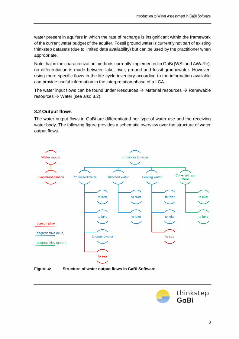
3.2 Output flows

The water output flows in GaBi are differentiated per type of water use and the receiving

water body. The following figure provides a schematic overview over the structure of water

output flows.

Figure 4: Structure of water output flows in GaBi Software


9

Water vapour and evapotranspiration are emissions to air and the typical form of consump-

tive water use.

Water vapour: water evaporated from a process.

Evapotranspiration: refers to water use in crop systems. More precisely, evapotranspiration

is defined as the combination of two separate processes whereby water is lost on the one

hand from the soil surface by evaporation and on the other hand from the crop by transpi-

ration.

Water that is not evaporated is usually emitted back to a water body. In GaBi the water

output flows to water are differentiated per source process and receiving water body.

Processed water: usually refers to waste water after treatment. This flow explicitly does not

make any reference to the quality of the released water. The flow is used as the elementary

output flow from waste water treatment processes in the GaBi processes, but can also be

used to refer to direct release of water into the environment without treatment. Emissions

of pollutants (chemical substances, nutrients etc.) should be assessed as separate output

flows in the inventory. Processed water can be released to a river, a lake and the sea.

Please note that the sea is not considered part of the watershed, and release to the sea is

counted as consumptive use.

Turbined water: refers to the release of water from turbines, i.e. hydroelectricity generation.

The differentiation between processed water and turbined water is important, because

some impact assessment methods do not consider water use from turbines (Resource de-

pletion water, midpoint (v1.09)).

Cooling water: refers to water used in cooling processes. The differentiation between pro-

cessed water and turbined water is mainly done for interpretational reasons. Cooling water

is usually not changed in quality but might influence ecosystems in through changes in

temperature, a potential impact not covered by the common impact categories.

Collected rain: water is used in cases where rain water is collected and returned to the

watershed, e.g. in large industrial plants with a large area of sealed surface, where the

precipitation needs to be directed into a waste water treatment. Those flows could of course

also be used to model rain water output after intentional rainwater harvesting. Please note


10

that these flows should be related to rain water as an input, and are not considered in blue

water use or consumption.

3.3 Additional water flows in GaBi

There are many more water flows in GaBi than those mentioned above. Most of them are

relating to operating materials, i.e. non-elementary flows that are output from one process

and input to another. Examples are “water (process water)” or “water (tap water)”. They may

be used in any model but must be connected to the respective delivering process.

Water (sea water) and water (brackish water) are elementary input flows but do not fall

under the definition of fresh water, therefore are not consider in the water assessment quan-

tities. A rare exception might be cases where seawater is treated and released as freshwa-

ter, but not back to the sea, which would result in a negative fresh water consumption.

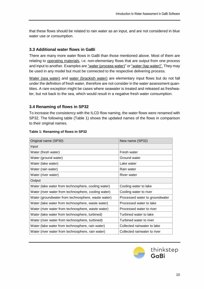
3.4 Renaming of flows in SP32

To increase the consistency with the ILCD flow naming, the water flows were renamed with

SP32. The following table (Table 1) shows the updated names of the flows in comparison

to their original names.

Table 1: Renaming of flows in SP32

Original name (SP30) New name (SP32)

Input

Water (fresh water) Fresh water

Water (ground water) Ground water

Water (lake water) Lake water

Water (rain water) Rain water

Water (river water) River water

Output

Water (lake water from technosphere, cooling water) Cooling water to lake

Water (river water from technosphere, cooling water) Cooling water to river

Water (groundwater from technosphere, waste water) Processed water to groundwater

Water (lake water from technosphere, waste water) Processed water to lake

Water (river water from technosphere, waste water) Processed water to river

Water (lake water from technosphere, turbined) Turbined water to lake

Water (river water from technosphere, turbined) Turbined water to river

Water (lake water from technosphere, rain water) Collected rainwater to lake

Water (river water from technosphere, rain water) Collected rainwater to river


11

4 Regionalization

4.1 Regionalized flows in GaBi

As mentioned in chapter 2.2, the impact assessment of water consumption needs to take

the location of water consumption into consideration.

In a first step, regionalization in GaBi is implemented on country level. Meaning that for

each elementary flow listed above, a regional copy exists specifying the country where the

water is used. The below table gives an example:

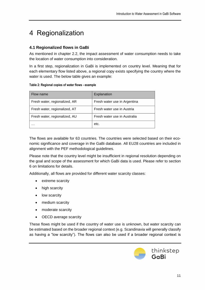
Table 2: Regional copies of water flows - example

Flow name Explanation

Fresh water, regionalized, AR Fresh water use in Argentina

Fresh water, regionalized, AT Fresh water use in Austria

Fresh water, regionalized, AU Fresh water use in Australia

… etc.

The flows are available for 63 countries. The countries were selected based on their eco-

nomic significance and coverage in the GaBi database. All EU28 countries are included in

alignment with the PEF methodological guidelines.

Please note that the country level might be insufficient in regional resolution depending on

the goal and scope of the assessment for which GaBi data is used. Please refer to section

6 on limitations for details.

Additionally, all flows are provided for different water scarcity classes:

extreme scarcity

high scarcity

low scarcity

medium scarcity

moderate scarcity

OECD average scarcity

These flows might be used if the country of water use is unknown, but water scarcity can

be estimated based on the broader regional context (e.g. Scandinavia will generally classify

as having a “low scarcity”). The flows can also be used if a broader regional context is


12

implicitly intended, i.e. “medium scarcity” to represent European average conditions. Addi-

tionally, these flows can also be used if the location of water use (and its respective water

scarcity) is known on a higher resolution than country level. An example would be water

use in the US, where some federal states have a low to moderate water scarcity while others

show high to extreme water scarcity, so those flows could be used rather than the US av-

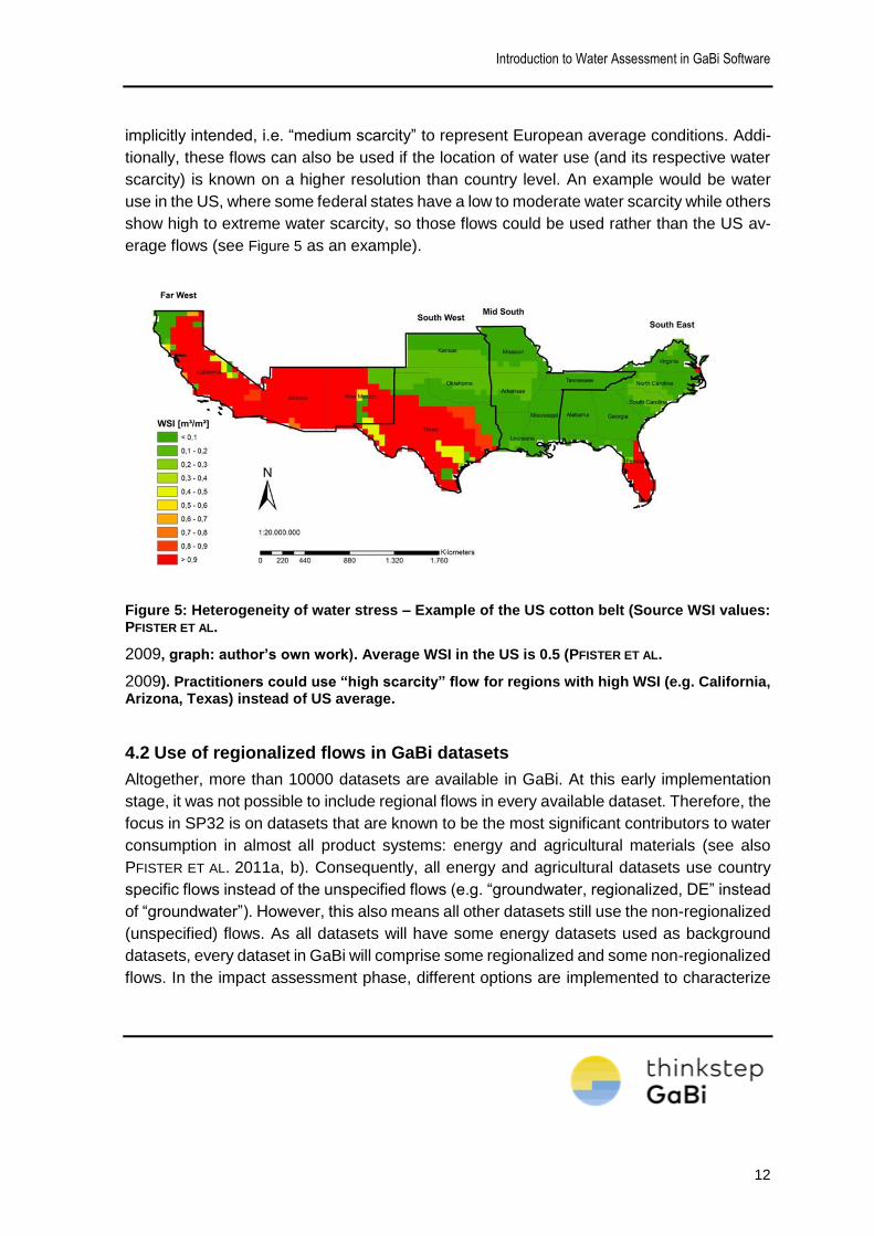
erage flows (see Figure 5 as an example).

Figure 5: Heterogeneity of water stress – Example of the US cotton belt (Source WSI values: PFISTER ET AL.

2009, graph: author’s own work). Average WSI in the US is 0.5 (PFISTER ET AL.

2009). Practitioners could use “high scarcity” flow for regions with high WSI (e.g. California, Arizona, Texas) instead of US average.

4.2 Use of regionalized flows in GaBi datasets

Altogether, more than 10000 datasets are available in GaBi. At this early implementation

stage, it was not possible to include regional flows in every available dataset. Therefore, the

focus in SP32 is on datasets that are known to be the most significant contributors to water

consumption in almost all product systems: energy and agricultural materials (see also

PFISTER ET AL. 2011a, b). Consequently, all energy and agricultural datasets use country

specific flows instead of the unspecified flows (e.g. “groundwater, regionalized, DE” instead

of “groundwater”). However, this also means all other datasets still use the non-regionalized

(unspecified) flows. As all datasets will have some energy datasets used as background

datasets, every dataset in GaBi will comprise some regionalized and some non-regionalized

flows. In the impact assessment phase, different options are implemented to characterize


13

these unspecified flows (see section 5.3). The interpretation of the results needs to take this

into account (see section 6 on limitations).


14

5 Impact Assessment – Water quantities in GaBi

The GaBi software contains inventory quantities for water use and water consumption, as

well as the impact assessment quantities, WSI, AWaRe, and UBP (see section 2.2), as

defined and described below.

5.1 Water use

The water input flows in GaBi refer to total water use. To quantify total freshwater use, all

freshwater input flows are summed up. As stated previously, rain water is important for a

complete inventory and thus part of the total water use and total freshwater use. However,

for impact assessments, only blue water (surface and groundwater) is considered, exclud-

ing rain water (see above footnote 1). Normally, the focus lies in freshwater use and con-

sumption. Sea water is also excluded in this aggregation. Thus, the flow based equations

are:

Total freshwater use = total freshwater withdrawal/abstraction

= Fresh water + Ground water + Lake water (incl. turbined) +

River water (incl. turbined) + water (fossil groundwater) + Rain

water

Blue water use = Fresh water + Ground water + Lake water (incl. turbined)

+ River water (incl. turbined) + water (fossil groundwater)

5.2 Water consumption

As mentioned above (see 2.1), freshwater that leaves the watershed is considered con-

sumed. This is the fraction that is most interesting as this water is lost to the ecosystem and

for downstream users.


15

Total freshwater consumption is defined as4:

Total freshwater consumption = total freshwater use (water input) – total freshwater

release back to watershed (degradative water outputs)

= Fresh water + Ground water + Lake water (incl. tur-

bined) + River water (incl. turbined) + water (fossil

groundwater) + Rain water - Cooling water to lake -

Cooling water to river - Processed water to groundwa-

ter - Processed water to lake - Processed water to river

- Turbined water to lake - Turbined water to river - Col-

lected rainwater to river - Collected rainwater to lake

In the respective GaBi quantity, this calculation approach is implemented by summing up

all inputs (characterization factor 1) and then subtracting all degradative output flows (char-

acterization factor -1).

Please note that in general, only blue water (surface and ground water) is considered.

Therefore, rain water is typically excluded from freshwater consumption and the focus is

only on blue water consumption (see above, footnote 1). In detail, the flow based calculation

is:

Blue water consumption = Fresh water + Ground water + Lake water (incl. tur-

bined) + River water (incl. turbined) + water (fossil

groundwater) - Cooling water to lake - Cooling water to

river - Processed water to groundwater - Processed water

to lake - Processed water to river - Turbined water to lake

- Turbined water to river

5.3 Water scarcity footprint (WSI, AWaRe, UBP)

The WSI, AWaRe and UBP quantities are based on the water consumption, i.e. the same

calculation logic (inputs – degradative outputs) applies. However, in these quantities the

flows are multiplied with the country specific characterization factors.

The quantities for WSI and AWaRe can be found under Environmental quantities water,

the UBP quantity under Environmental quantities UBP 2013.

4 Please note that this quantity corresponds to the “blue water footprint” plus “green water footprint” as proposed by the Wa-

ter Footprint Network (WFN). The WFN used the term “water footprint” different than ISO 14046, as regionalized impact assessment is not part of the water footprint according to the WFN.


16

For WSI, the resulting unit is water deprivation (in m³) or “RED” water (Relevant environ-

mental depletion, see Pfister 2009)5. For AWaRe, the resulting unit is “User Deprivation

Potential” (UDP) in m³ world-equivalents. For UBP, the resulting unit are points of Eco Scar-

city.

High, OECD+BRIC average and low characterization factor for unspecified water

The WSI and AWaRe quantities exist in three different versions, with a high, OECD+BRIC

average, and low characterization factor for unspecified water. In these quantities, all char-

acterization factors are the same, except those for the unspecified (non-regionalized) flows.

As described in section 0, the unspecified (non-regionalized) flows are still used in many

data sets. For those flows, different characterization factors are used in the different quan-

tities. In the version “high”, the unspecified flows are characterized with a high scarcity factor

- choosing this quantity assumes “unspecified water” is consumed in water stressed re-

gions, such as the Middle East or Spain. The “OECD+BRIC average” version refers to the

average water scarcity in the OECD + BRIC countries. This value was preferred over the

global average (all countries) as the OECD + BRIC represent the majority of worldwide

economic activity. The “low” version represents less water stressed countries, such as in

North-Western Europe.

As mentioned in section 2.2, additional to those consumption-based methods, two other

water assessment methods are available in GaBi (ReCiPe 1.08 water depletion, and Re-

source depletion water, mid-point v1.09). The quantities are based on water use; therefore,

they only consider water input flows6.

5 Ridoutt & Pfister 2010 recommend to apply normalisation to water deprivation (water consumption x WSI), This normaliza-

tion is conducted using the global average water stress (0.602). The resulting unit is m³ of water equivalents (m³ water eq.) The interpretation of this value is 1kg water as “if it was consumed on a global level”. If users prefer to use this value, they need to divide the value provided by the WSI quantity by 0.602 (global average scarcity factor).

6 Resource depletion water, mid-point v1.09 does not include turbined water


17

6 Limitations

Regionalized impact assessment is a comparatively new field in practical LCA work. The

GaBi 2017 databases are ground-breaking in being among the first to implement regional-

ized impact assessment into a generic LCA database. However, it should be kept in mind

that many published methods focus on specific modelling situations where detailed data is

available (e.g. agricultural cultivation on a specific field in a specific region). Applying these

methods to generic databases is complex in terms of the technical implications but also in

terms of data availability. For some datasets, the specific region is unknown. For others, it

is explicitly intended to represent regional averages (e.g. fertilizers in the EU). Others will

represent averages, but with specific regional context (e.g. for generation of hydropower,

several dams in specific water sheds from the country average).

Therefore, the implementation of water assessment in GaBi is subject to limitations

that should be kept in mind when interpreting the results:

For both WSI and AwaRe, the method developer provided characterization factors on

water shed level, which is seen as the appropriate spatial resolution for water assess-

ments. However, most LCA datasets are organized on country level. The application

of characterization factors aggregated into country averages can lead to large uncer-

tainty in the obtained results, especially for large countries such as Brazil or the US,

where a wide range of regions with different scarcity levels are covered. Working with

the different scarcity classes in the flow classification (extreme to low) and the different

versions of the quantities (high, average, low for unspecified flows) should be used to

set up scenarios to better understand these uncertainties.

For an assessment of water scarcity, it is not only important where the water con-

sumption takes place, but also when. Many regions in the world are water abundant

in a certain period (e.g. rainy season) and extremely water stressed in another (e.g.

dry season). Temporal specific characterization factors are available for WSI and

AWaRe, but could not be implemented into GaBi due to the structure of the datasets

and limited data availability. Though it should be noted that temporal variation in water

availability is considered in the aggregated characterization factors to some extend

(see Pfister 2009 and AWaRe documentation7).

In AWaRe, three different use classes are differentiated: agricultural water use, non-

agricultural water use, and unspecified water use (the latter being the consumption

weighted average of the two). Due to technical reasons, at this stage, only the char-

acterization factors for unspecified flows are implemented into GaBi. The values for

7 http://www.wulca-waterlca.org/project.html

http://www.wulca-waterlca.org/project.html


18

these characterization factors are usually closer to those for agriculture and thus

higher than those for non-agricultural use. Consequently, in the current state of the

implementation into GaBi, the AWaRe results for industrial processes are likely to be

lower if the non-agricultural characterization factors are used (future implementation

discussed)

As described in section 0, only the energy datasets and agricultural materials use

regionally specific water flows (SP 32). While these processes will cover the largest

fraction of water consumption in most production systems, potentially a significant

fraction of water consumption remains unspecified and is subject to large uncertainty

regarding water scarcity. The different versions of the WSI and AWaRe quantities

(high, average, low for unspecified flows) should be used to set up scenarios to better

understand these uncertainties.

Nevertheless, it is important to understand that water scarcity footprint values provided in

GaBi should be considered to be a good starting point in water assessment, and not as the

terminal stop. Absolute numbers should be interpreted with care. The GaBi assessment

should preferably be used for hot-spot analysis, which proved to be fairly robust despite the

above-mentioned limitations. A refined analysis of the determined hotspots can add valua-

ble information and improve the reliability of the results (see BUXMANN ET AL. 2016 as an

example for such a stepwise approach).


19

7 Literature

BAYART ET AL.

2010

BAYART, J.; BULLE, C.; DESCHÊNES, L.; MARGNI, M; PFISTER, S.; VINCE, F.; KOEHLER, A. (2010): A FRAMEWORK FOR ASSESSING OFF-STREAM

FRESHWATER USE IN LCA. INT J LIFE CYCLE ASSESS 17(3), PP 304-313

BUXMANN ET AL. 2016 BUXMANN K, KOEHLER A, THYLMANN D. WATER SCARCITY FOOTPRINT

OF PRIMARY ALUMINIUM. INT. J. LIFE CYCLE ASSESS. 2016:1–11

FRISCHKNECHT &

KNÖPFEL 2013 FRISCHKNECHT R., BÜSSEL KNÖPFEL, S. (2013): SWISS ECO-FACTORS

2013 ACCORDING TO THE ECOLOGICAL SCARCITY METHOD, FEDERAL

OFFICE FOR THE ENVIRONMENT FOEN, ÖBU - WORKS FOR SUSTAINABIL-

ITY, BERN

ISO 14046 ISO/CD LIFE CYCLE ASSESSMENT -- WATER FOOTPRINT -- REQUIRE-

MENTS AND GUIDELINES. INTERNATIONAL ORGANIZATION FOR

STANDARDIZATION, 2014.

PFISTER ET AL.

2009

PFISTER, S.; KOEHLER, A.; HELLWEG, S. (2009): ASSESSING THE ENVI-

RONMENTAL IMPACT OF FRESHWATER CONSUMPTION IN LCA. ENVIRON

SCI TECHNOL 43(11), 4098–4104.

PFISTER ET AL. 2011A PFISTER S, SANER D, KOEHLER A. THE ENVIRONMENTAL RELEVANCE OF

FRESHWATER CONSUMPTION IN GLOBAL POWER PRODUCTION. INT. J. LIFE CYCLE ASSESS. 2011;16(6):580–91

PFISTER ET AL. 2011B STEPHAN PFISTER, PETER BAYER, ANNETTE KOEHLER, AND STEFANIE

HELLWEG (2011): ENVIRONMENTAL IMPACTS OF WATER USE IN GLOBAL

CROP PRODUCTION: HOTSPOTS AND TRADE-OFFS WITH LAND USE, EN-

VIRONMENTAL SCIENCE & TECHNOLOGY 2011 45 (13)

RIDOUTT, PFISTER

2010

RIDOUTT, B.; PFISTER, S. (2010): A REVISED APPROACH TO WATER FOOT-

PRINTING TO MAKE TRANSPARENT THE IMPACTS OF CONSUMPTION AND

PRODUCTION ON GLOBAL FRESHWATER SCARCITY. GLOBAL ENVIRON-

MENTAL CHANGE 20 (2010), 113–120

SALA ET. AL 2016 S SALA, L BENINI, B VIDAL, V CASTELLANI, R PANT (2016): ENVI-

RONMENTAL FOOTPRINT - UPDATE OF LIFE CYCLE IMPACT ASSESSMENT

METHODS; DRAFT FOR TAB; (STATUS: MAY 2, 2016); AA JRC NO

33446 – 2013-11 07.0307/ENV/2013/SI2.668694/A1

introduction to water assessment in gabi software · introduction to water assessment in gabi...

Documents