introduction to matlab programming -...

Introduction to Scientific Computing and Data Analysis by M. Holmes (Springer, 2016)

Appendix D

Introduction to MATLAB

Programming

Contents

D.1 Getting Started . . . . . . . . . . . . . . . . . . . . . . . . . . . . . 2

D.2 Basic m-file . . . . . . . . . . . . . . . . . . . . . . . . . . . . . . . . 3

D.2.1 Printing . . . . . . . . . . . . . . . . . . . . . . . . . . . . . . . . . . 5

D.3 Basic Plotting . . . . . . . . . . . . . . . . . . . . . . . . . . . . . . 7

D.3.1 Legends . . . . . . . . . . . . . . . . . . . . . . . . . . . . . . . . . . 8

D.3.2 Saving and Printing Plots . . . . . . . . . . . . . . . . . . . . . . . . 9

D.4 If/Else/Break/Return . . . . . . . . . . . . . . . . . . . . . . . . . . 10

D.5 Function Programs . . . . . . . . . . . . . . . . . . . . . . . . . . . 11

D.6 Entering Matrices and Vectors . . . . . . . . . . . . . . . . . . . . 13

D.6.1 Row and Column Manipulation . . . . . . . . . . . . . . . . . . . . . 14

July 23, 2017

The following is a brief introduction to using MATLAB. This is not intended to providea listing of various MATLAB commands, but illustrate how simple MATLAB programs arewritten, and the output displayed and printed. The goal is to get you started, and to alsoprovide enough information that you can use the very good help facility that comes withMATLAB (most people who use MATLAB make frequent use of the help pages). It is alsoassumed that you have a basic, but perhaps imperfect, understanding of coding. This meansthat you are aware that there are such things as for-loops and if/then/else type statements,although unclear of their exact formatting. Finally, for many of the commands or actionsthat are considered, there are likely other ways to accomplish the same thing. Some of thempossibly simpler, or maybe more clever, than what is shown here.

Caveat: The examples are worked out using a Mac implementation of MATLAB. It’s assumedsimilar responses are obtained using other implementations.

1


D.1 Getting Started

The tool bar and window arrangement when you start MATLAB are shown in Figure D.1.The worksheet area, what is called the Command Window, is seen and it contains the �prompt. Commands can be typed directly into the worksheet, including comment lines. Ofmore interest here are when the commands are contained in an m-file, and the file run asa program. How this is done is explained shortly, but it is first necessary to tell MATLABwhere the files are located. As you can see in Figure D.1, right above the Command Window,the current folder is identified. In this case it is the Desktop folder. Just to the left ofthe Command Window the contents of the current folder are listed. The m-files needed forthis Appendix are contained in the folder Appendix4/m files, and this is selected to run thevarious examples used here.

Figure D.1: Typical (default) MATLAB window.

After changing the current folder to Appendix4/m files, there is a list of the m-files onthe left (similar to the list shown in Figure D.1). The first example to be discussed is inthe m-file ss.m. Clicking on this, the result is shown in Figure D.2 (only the fist line ofss.m is shown). As you see, when the m-file is opened, its contents are shown in the Ed-

itor window. The Command Window is below this window (and is not shown in FigureD.2). Note the little red box, which contains an inverted triangle. This triangle lets you sep-arate a window from the others (this is useful depending on the size of your computer screen).

Figure D.2: The Editor window, and the first line of the m-file ss.m.

2


D.2 Basic m-file

To begin, in the textbook, in Example 1 in Section 1.1, the sum

S(n) =nX

j=1

1

j

(D.1)

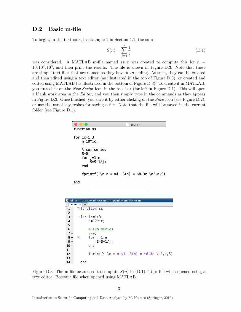
was considered. A MATLAB m-file named ss.m was created to compute this for n =10, 102, 103, and then print the results. The file is shown in Figure D.3. Note that theseare simple text files that are named so they have a .m ending. As such, they can be createdand then edited using a text editor (as illustrated in the top of Figure D.3), or created andedited using MATLAB (as illustrated in the bottom of Figure D.3). To create it in MATLAB,you first click on the New Script icon in the tool bar (far left in Figure D.1). This will opena blank work area in the Editor, and you then simply type in the commands as they appearin Figure D.3. Once finished, you save it by either clicking on the Save icon (see Figure D.2),or use the usual keystrokes for saving a file. Note that the file will be saved in the currentfolder (see Figure D.1).

Figure D.3: The m-file ss.m used to compute S(n) in (D.1). Top: file when opened using atext editor. Bottom: file when opened using MATLAB.

3


A synopsis of the commands in ss.m is given below.

for-loop with index ic

comment line

for-loop used to compute series

print values of n and S

A couple of additional comments related to the commands used.

for-loops: The for-loop starting on line 3 uses the values 1, 2, 3 (in that order). If youwanted the values to increase by, say, 4 each time, then ic = 1:3 is replaced with ic =1:4:13. With this, the values for ic are 1, 5, 9, 13. Similarly, suppose you wanted touse, in order, 7, 5, 3, 1. In this case ic = 1:3 is replaced with ic = 7:�2:1. Note thatthere are also while-loops, which are very useful, and an example is given in Section D.5.

fprintf : This command contains the formatting to be used, with n written in integer formatand S in exponential format. By default, the output appears in the Command Window.To find out about the format options, consult the help page for fprintf.

To run the commands in ss.m, with the file open in the Editor window, click on thegreen Run icon (see Figure D.2). The output appears in the Command Window, and whatis computed is shown in Figure D.4. The green comment line was typed directly into theCommand Window after the program was run (this is useful for annotating the output whenit is to be submitted as homework).

Figure D.4: Output from the ss.m file, along with a comment added afterward.

4


D.2.1 Printing

What is considered next are ways to print MATLAB files as well as the output. The easiestway is to use the Publish command, but there are other possibilities for specific tasks andthese are described as well.

Figure D.5: Publish tab used to print MATLAB files.

Publish Command

With the m-file open, the Publish tab is selected (see Figure D.5). You simply click on thegreen triangle on the right to run the Publish command. What you get depends on what youhave selected for the Publishing Options. Using the default settings, you will get a web-page(html file) which includes a copy of the m-file as well as the output, and this is easily printed.However, there are other possible outcomes, and some of the more useful are listed below.

Only m-file: Change option “Evaluate code:true” to “Evaluate code:false”.

Only output: Change option “Include code:true” to “Include code:false”.

PDF file: Change “Output file format:html” to “Output file format:pdf”.

Worth mentioning: There is an auto-formatting command that makes reading an m-filemuch easier. This is done in the Editor window by selecting the text of the file and thenclicking on the green page icon just to the right of the word Indent on the tool bar (see FigureD.2).

Limitation: The Publish command prints the file that is currently open, and will not printother files that might be used by the code. If you want them printed then they must be doneseparately or else included in the open file as local functions (these are explained in SectionD.5).

5


Non-Publish Methods

m-file: The contents of an m-file can be printed using LaTeX. There is a LaTeX option forPublish, but a better approach is to use the matlab-prettifier package. An example isgiven in the figure below, which contains the LaTeX commands to print ss.m. Note thatwhen the document is created, the TeX previewer reads the m-file, which is located bypathname (line 4). Moreover, it’s possible to include text and mathematical expressionsin the document, which is useful for producing homework write-ups and other technicaldocuments.

Finally, it is possible to print an m-file by simply using the keystrokes usually used forprinting a file (on a Mac this is Command-P). This is a few milliseconds faster thanusing the Publish method, but what you get in this case is a full page, large format,printout of the file.

Output : As illustrated in Figures D.3 and D.4, the fprintf command can be used to generateformatted output in the Command Window. It’s possible to write it to a text file instead(which are easily printable as well as editable). Assuming the name of the text file isdata.txt, then the commands shown in the figure below will work. Specifically, the fileis created (line 3), written into (line 13), and then closed (line 16).

6


D.3 Basic Plotting

A basic m-file, named p.m, that plots y = cos(x) for 0 x 2⇡ is shown in the top rowin Figure D.6. To compute the curve, 100 points are used along the x-axis. The fact isthat the resulting plot is rather poor, and unacceptable for publication. For example, thetext is almost unreadable, and the curve is very light. This is easily fixed, and the modifiedfile, named pp.m, is shown in second row of Figure D.6. What was done was to change theline width for the curve (line 14), and to change the font properties used for labeling (line20). There is considerable flexibility to modify the plot parameters, and the help pages forthe plot command should be consulted. Also, in terms of the font size used in a plot, itis worth knowing that in publishing it is generally expected that the font size in the plotapproximately matches the size used in the text.

0 1 2 3 4 5 6 7x-axis

-1

-0.8

-0.6

-0.4

-0.2

0

0.2

0.4

0.6

0.8

1

y-axis

0 1 2 3 4 5 6 7x-axis

-1

-0.5

0

0.5

1

y-axis

Figure D.6: The commands on the left produce the plot on the right.

7


D.3.1 Legends

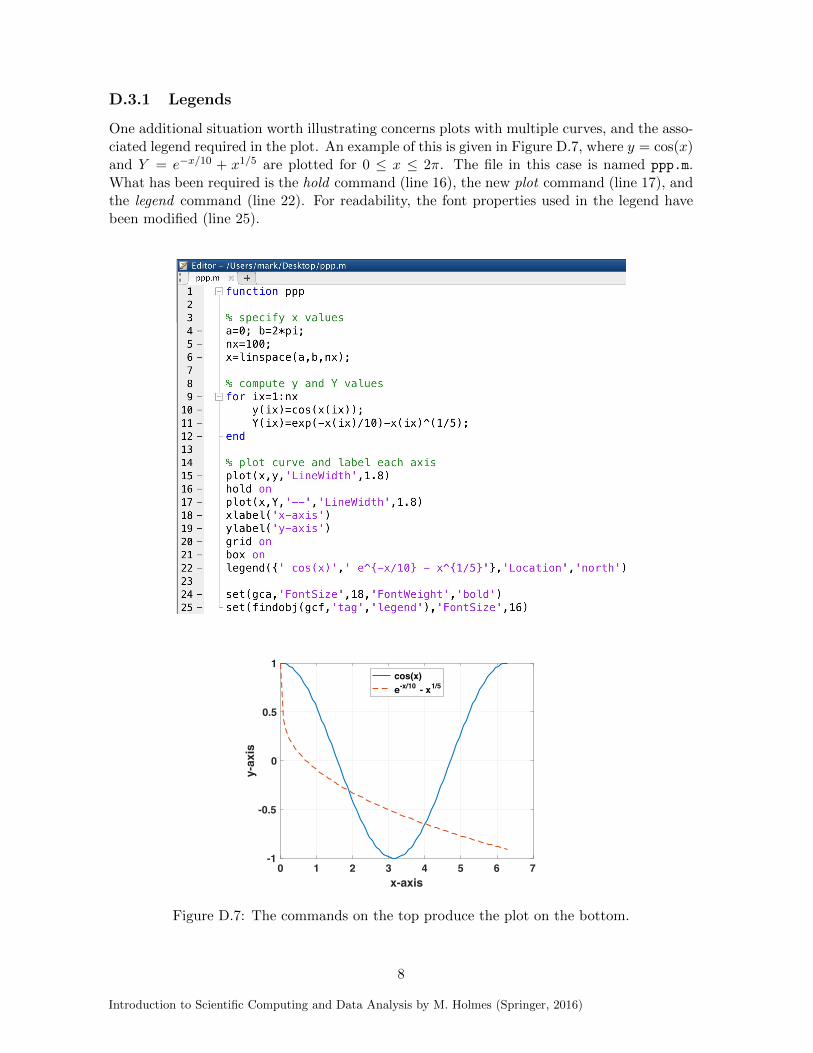
One additional situation worth illustrating concerns plots with multiple curves, and the asso-ciated legend required in the plot. An example of this is given in Figure D.7, where y = cos(x)and Y = e

�x/10 + x

1/5 are plotted for 0 x 2⇡. The file in this case is named ppp.m.What has been required is the hold command (line 16), the new plot command (line 17), andthe legend command (line 22). For readability, the font properties used in the legend havebeen modified (line 25).

0 1 2 3 4 5 6 7x-axis

-1

-0.5

0

0.5

1

y-ax

is

cos(x) e-x/10 - x1/5

Figure D.7: The commands on the top produce the plot on the bottom.

8


D.3.2 Saving and Printing Plots

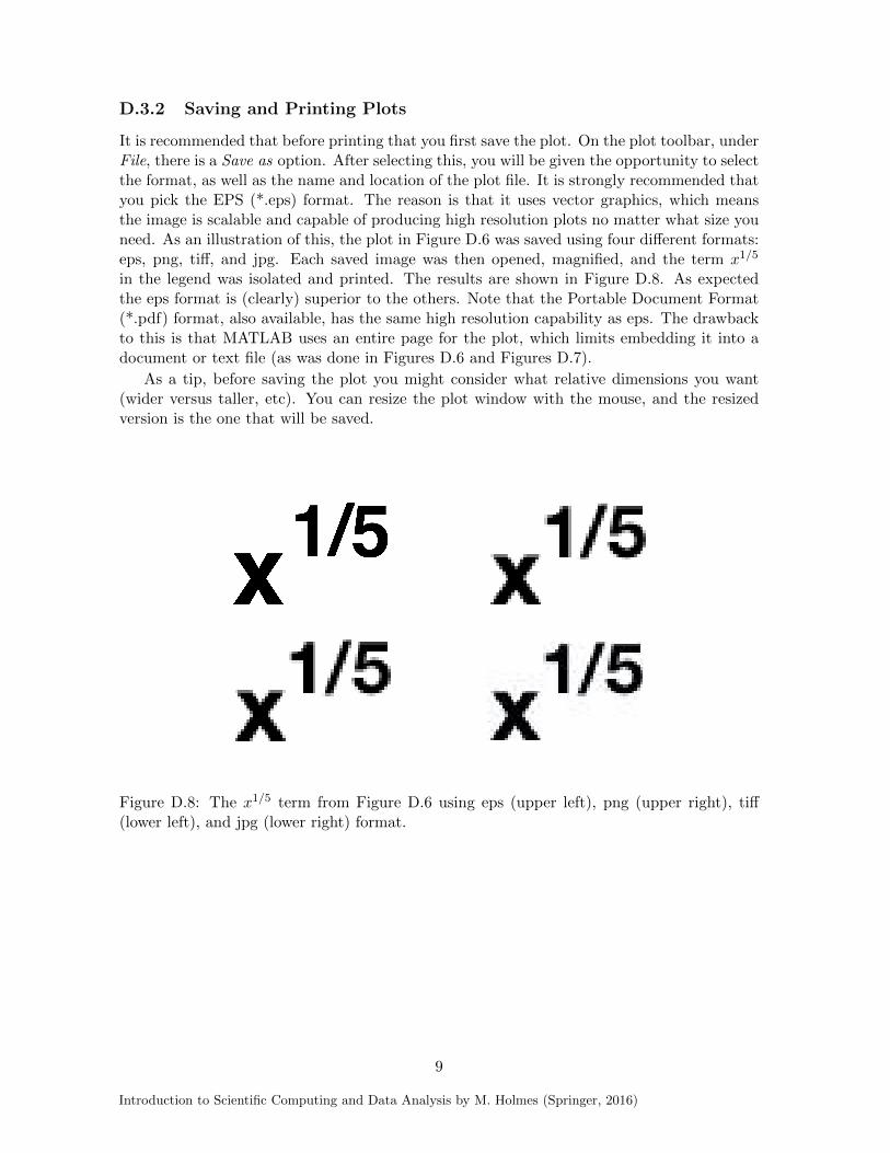
It is recommended that before printing that you first save the plot. On the plot toolbar, underFile, there is a Save as option. After selecting this, you will be given the opportunity to selectthe format, as well as the name and location of the plot file. It is strongly recommended thatyou pick the EPS (*.eps) format. The reason is that it uses vector graphics, which meansthe image is scalable and capable of producing high resolution plots no matter what size youneed. As an illustration of this, the plot in Figure D.6 was saved using four di↵erent formats:eps, png, ti↵, and jpg. Each saved image was then opened, magnified, and the term x

1/5

in the legend was isolated and printed. The results are shown in Figure D.8. As expectedthe eps format is (clearly) superior to the others. Note that the Portable Document Format(*.pdf) format, also available, has the same high resolution capability as eps. The drawbackto this is that MATLAB uses an entire page for the plot, which limits embedding it into adocument or text file (as was done in Figures D.6 and Figures D.7).

As a tip, before saving the plot you might consider what relative dimensions you want(wider versus taller, etc). You can resize the plot window with the mouse, and the resizedversion is the one that will be saved.

Figure D.8: The x

1/5 term from Figure D.6 using eps (upper left), png (upper right), ti↵(lower left), and jpg (lower right) format.

9


D.4 If/Else/Break/Return

Conditionals are often needed, and can involve a wide variety of conditions or outcomes. Thisrequires knowing how relational and logical operators are written. Examples of some of themore often used possibilities are illustrated in the figure below. For more information aboutthese, look at relational operations and logical operations in MATLAB’s help pages.

Generate some random integers

Compute f if x > y

Compute g if x � y and z = 1

Otherwise, compute g if x 6= 2 or y z

Otherwise, use this formula for g

If x < 5 stop computing and leave function

Otherwise, if x < w then leave the for-loopand go to next command (line 30)

A few additional comments are in order. First, in the compound version (as in lines 13-19)it is possible to have multiple elseif conditions, and to not have an else condition. It isalso possible to have more than two tests for an if or elseif condition. If this is done, it’simportant to group the tests based on what is being required. For example, the tests

x � y or (x ⇤ y > 50 and z > 8)

can produce a di↵erent result from

(x � y or x ⇤ y > 50) and z > 8.

Finally, as the latter tests indicate, it is possible to have arithmetic expressions as part of atest.

10


D.5 Function Programs

The first line of the m-file ss.m, shown in Figure D.3, is function ss. The other m-filesthat have been considered begin in a similar manner. The reason for doing this is that bydeclaring it a function program, all of the variables that are defined in the program arekept separate from other calculations that have been, or will be, done by MATLAB in theCommand Window. What is considered now is how to pass information between functionprograms, and to consider some of the reasons why you might want to do this.

Consider the secant method to solve f(x) = 0, which according to (2.24), gives rise to theequation

x

i+1 = x

i

� f(xi

)(xi

� x

i�1)

f(xi

)� f(xi�1)

, for i = 1, 2, · · · .

A function program for this is shown in the figure below (the algorithm is a modified versionof the one appearing in Table 2.6). It is not necessary to understand the various steps in

this program, other than it requires (in lines 4 and 9) the evaluation of f(x). This is goingto be done using another function program, and we want the value to be accessible to oursecant program. As an example, suppose f(x) = 3 cos(2⇡x)�4x. The corresponding functionprogram is shown below. The only remaining question is, where does this second function

go? Some like one function per m-file, and so they would put it in a file named f.m. It is alsopossible to include it at the end of the m-file that contains the secant1 function. The lattermethod is used with many of the m-files included with the textbook because it results in aself-contained file. In doing this, the first function is the main function, and is the one thatMATLAB associates with the file name. Subsequent functions in the m-file are called local

functions and they are only available to the other functions within that file.

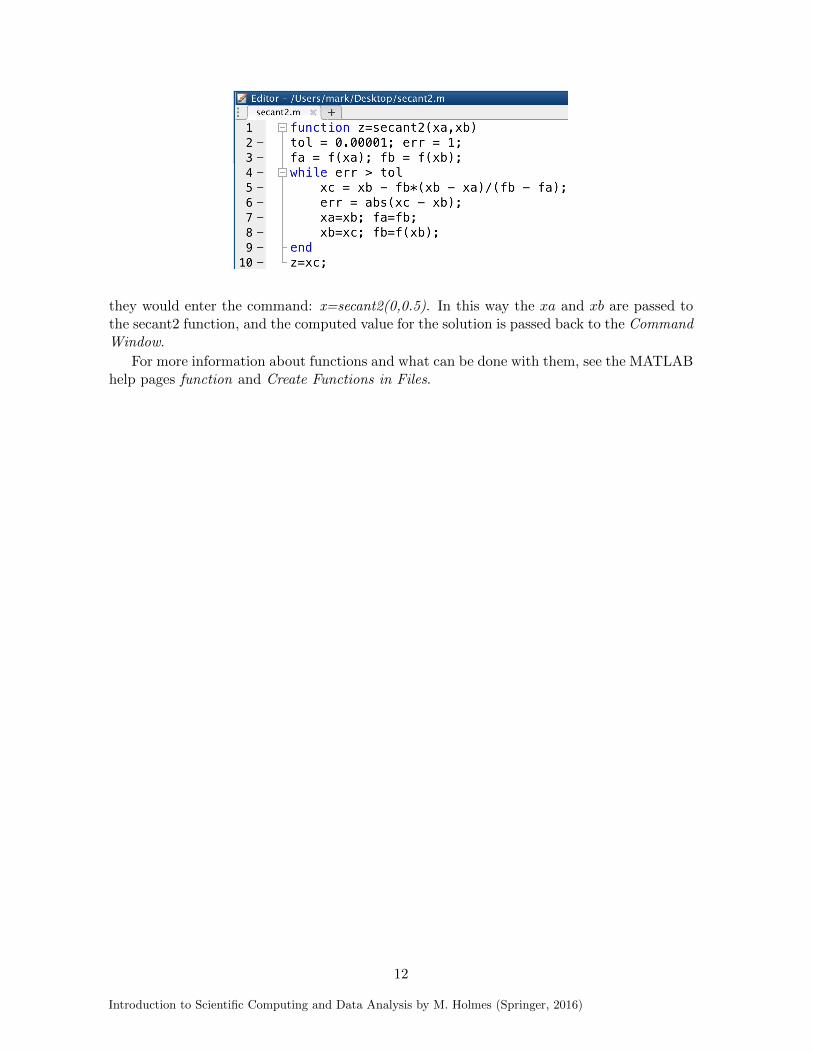
To illustrate another possibly, suppose you want to have a general purpose secant methodsolver. The idea is that the user would provide the f.m file and the two starting values xa andxb, and then would find the solution by issuing the command secant2(xa,xb). This requires afew small adjustments to secant1.m, and the result is shown in the figure below (the modifiedfile is named secant2.m). If one takes xa = 0 and xb = 0.5, then in the Command Window

11


they would enter the command: x=secant2(0,0.5). In this way the xa and xb are passed tothe secant2 function, and the computed value for the solution is passed back to the Command

Window.

For more information about functions and what can be done with them, see the MATLABhelp pages function and Create Functions in Files.

12


D.6 Entering Matrices and Vectors

Generally, the problems solved numerically are large enough that entering matrices and vec-tors by hand is impractical. Instead, for-loops or specialized commands are employed. Whatis described below are some of the ways to do this.

The most versatile way to enter a matrix is using nested for-loops. To illustrate, forthe n ⇥m Vardermonde matrix V in Section 8.3, V

ij

= (1/i)j�1. In MATLAB, assuming n

and m have been specified, this can be entered using the commands shown in the figure below.

V =

0

BBBBBBBBB@

1 1 1 . . . 1

1 1/2 (1/2)2 . . . (1/2)m�1

......

......

1 1/n (1/n)2 . . . (1/n)m�1

1

CCCCCCCCCA

This works for all matrices, with line 3 changed accordingly. Vectors can be entered similarly,using a single for-loop. What needs to be done is to indicate whether it is a column or rowvector. To illustrate, suppose the ith entry in a vector x is x

i

= 1/i. How to enter this asa column or row vector is shown in the figures below (it is assumed n has been specified).For other vectors, line 3 would change accordingly. Also, to switch between row and columnformat just use the MATLAB’s transpose command: x0.

x =

0

BBBBBBBBB@

1

1/2

...

1/n

1

CCCCCCCCCA

x =

✓1 1/2 . . . 1/n

◆

For a matrix with particular patterns in its entries, it is possible to use some of thespecialized commands available in MATLAB. Of particular interest are the following matrixgenerating commands:

ones(n,m): This is an n⇥m matrix consisting of all ones.

zeros(n,m): This is an n⇥m matrix consisting of all zeros.

eye(n,m): This is an n⇥m matrix with ones along the main diagonal, and zeros elsewhere.

13


diag(v,k): This creates a zero matrix except that the vector v is placed on the kth diagonal(with k = 0 for main diagonal, k = 1 for the superdiagonal, k = �1 for the subdiagonal,etc). Note that the size of the resulting matrix depends on the size of v and the valueof k.

An an example, a tridiagonal matrix can be written as follows (it is assumed n is specified):0

BBBBB@

2 11 2 1

. . .. . .

. . .

11 2

1

CCCCCA=

0

BBBBB@

2 00 2 0

. . .. . .

. . .

00 2

1

CCCCCA+

0

BBBBB@

0 01 0 0

. . .. . .

. . .

01 0

1

CCCCCA+

0

BBBBB@

0 10 0 1

. . .. . .

. . .

10 0

1

CCCCCA

= 2 ⇤ eye(n, n) + diag(ones(n� 1, 1),�1) + diag(ones(n� 1, 1), 1)

The above formula might qualify for “advanced MATLAB,” in the sense that most casualusers would not know to use it. However, there is an alternative that most anyone under-stands. This involves using a single for-loop, and the commands are given in the figure below.

D.6.1 Row and Column Manipulation

An often useful command uses the colon (:) to access any particular row or column of amatrix. It is used in basically the same way that it is used in a for-loop, and in the figurebelow some of the possibilities are illustrated. The big di↵erence is when the colon is usedby itself (as in lines 4 and 6), which means that all possible index values are used.

Generate a random n⇥m matrix

Vector x is formed using the third column of A

Set the second row of A to all ones

In the fifth column of A, set rows 2, 3, 4 to zero

The vector y is formed from the fourth row ofA, using column entries, 1, 3, 5

14

introduction to matlab programming -...

Documents