Introduction to Location Discovery Lecture 9 October 5, 2006

EENG 460a / CPSC 436 / ENAS 960 Networked Embedded Systems &

Sensor Networks

Andreas Savvidesandreas.savvides@yale.edu

Office: AKW 212Tel 432-1275

Course Websitehttp://www.eng.yale.edu/enalab/courses/2006f/eeng460a

Lecture Outline

Programming assignment due next Tuesday• You should be making good progress with it!!!

Recap from last lecture Look at the multihop case Discuss an EKF solver Some words on bounds

Last Lecture Recap: Problem Formulation

Need to minimize the sum of squares of the residuals

The objective function is

This a non-linear optimization problem• Many ways to solve (e.g a forces formulation, gradient

descent methods etc

22,, )ˆ()ˆ( uiuiiuiu yyxxrf

2,min),( iuuu fyxF

Base Station 1

Base Station 3

Base Station 2

u

Two Possible Ways to Solve the Problem

1. Linearize by subtracting one equation from the rest

Solve the resulting set of linear equations

2. Linearize using Taylor Expansion

A Solution Suitable for an Embedded Processor

Linearize the measurement equations using Taylor expansion

where

Now this is in linear form

)( 22,, Oyxfr yixiiuiu

i

uii

i

uii r

yyy

r

xxx

ˆ,

ˆ

22 )ˆ()ˆ( uiuii yyxxr

zA

Solve using the Least Square Equation

The linearized equations in matrix form become

Now we can use the least squares equation to compute a correction to our initial estimate

Update the current position estimate

Repeat the same process until δ comes very close to 0

)(3

)(2

)(1

33

22

11

, ,u

u

u

y

x

f

f

f

z

yx

yx

yx

A

zAAA TT 1)(

yuuxuu yyxx ˆˆ and ˆˆ

The Multihop Problem

Beacon

Unkown Location

Randomly Deployed Sensor Network

Beacon nodes

• Localize nodes in an ad-hoc multihop network• Based on a set of inter-node distance measurements

Solving over multiple hops

Iterative Multilateration

Beacon node(known position)

Unknown node(known position)

Iterative Multilateration

Iterative Multilateration

ProblemsError accumulationMay get stuck!!!

% of initial beacons

Localized nodes

total nodes

Collaborative Mutlilateration

• All available measurements are used as constraints

• Solve for the positions of multiple unknowns simultaneously

• Catch: This is a non-linear optimization problem!

• How do we solve this?

Known position

Uknown position

Problem Formulation

214

2141,41,4

254

2545,45,4

234

2343,43,4

253

2535,35,3

232

2323,23,2

)ˆ()ˆ(

)ˆ()ˆ(

)ˆˆ()ˆˆ(

)ˆ()ˆ(

)ˆ()ˆ(

yyxxRf

yyxxRf

yyxxRf

yyxxRf

yyxxRf

2,4433 min)ˆ,ˆ,ˆ,ˆ( jifyxyxF

The objective function is

Can be solved using iterative least squares utilizing the initial Estimates from phase 2 - we use an Extended Kalman Filter

1

2

3 4

5

6

Things to look out for…

Iterative methods and gradient decent methods are not guaranteed to converge to the global minimum, it is very easy to get stack in local minima• To converge properly, you need to provide a

good set of initial estimates. In general this is not a problem with the 1-

hop setups but it becomes a big problem with multihop setups

How do we solve this problem?

In an embedded system? Backboard material here… One possible solution would use a Kalman

Filter• This was found to work well in practice, can

“easily” implemented on an embedded processor

[more details see Savvides03]

Computation Options

1. CentralizedOnly one node computes

2. Locally Centralized Some of unknown nodes compute

3. (Fully) DistributedEvery unknown node computes

Computing Nodes

• Each approach may be appropriate for a different application• Centralized approaches require routing and leader election• Fully distributed approach does not have this requirement

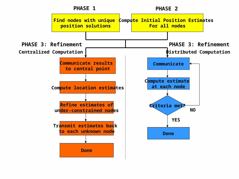
Find nodes with unique position solutions

Compute Initial Position Estimates For all nodes

Compute location estimates

Compute estimate at each node

Communicate

Criteria met?

YES

NO

Communicate results to central point

Transmit estimates back to each unknown node

Refine estimates ofunder-constrained nodes

Done

Done

Centralized Computation Distributed Computation

PHASE 1 PHASE 2

PHASE 3: Refinement PHASE 3: Refinement

Initial Estimates (Phase 2)

Use the accurate distance measurements to impose constraints in the x and y coordinates – bounding box

Use the distance to a beacon as bounds on the x and y coordinates

a

a ax

U

Initial Estimates (Phase 2)

Use the accurate distance measurements to impose constraints in the x and y coordinates – bounding box

Use the distance to a beacon as bounds on the x and y coordinates

Do the same for beacons that are multiple hops away

Select the most constraining bounds

a

b

c

b+c b+c

X

Y

U

U is between [Y-(b+c)] and [X+a]

Initial Estimates (Phase 2)

Use the accurate distance measurements to impose constraints in the x and y coordinates – bounding box

Use the distance to a beacon as bounds on the x and y coordinates

Do the same for beacons that are multiple hops away

Select the most constraining bounds

Set the center of the bounding box as the initial estimate

a

a a

b

c

b+c b+c

X

Y

U

Initial Estimates (Phase 2)

Example:• 4 beacons• 16 unknowns

To get good initial estimates, beacons should be placed on the perimeter of the network

Observation: If the unknown nodes are outside the beacon perimeter then initial estimates are on or very close to the convex hull of the beacons

Overview: Collaborative Multilateration

Collaborative Multilateration

ChallengesComputation constraintsCommunication cost

1

2

3

45

2

1

3

45

1

2

3

45

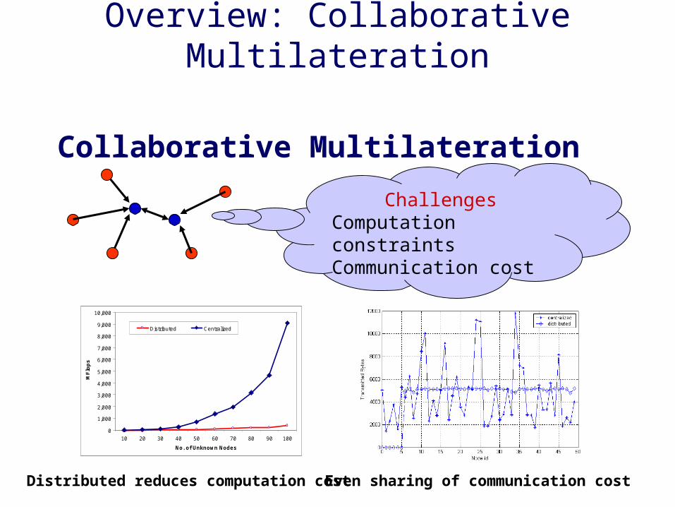
Overview: Collaborative Multilateration

Collaborative Multilateration

ChallengesComputation constraintsCommunication cost

0

1,000

2,000

3,000

4,000

5,000

6,000

7,000

8,000

9,000

10,000

10 20 30 40 50 60 70 80 90 100

No. of Unknown Nodes

MF

lop

s

Distributed Centralized

Distributed reduces computation cost Even sharing of communication cost

Satisfy Global Constraints with Local Computation

From SensorSim simulation 40 nodes, 4 beacons IEEE 802.11 MAC 10Kbps radio Average 6 neighbors per node

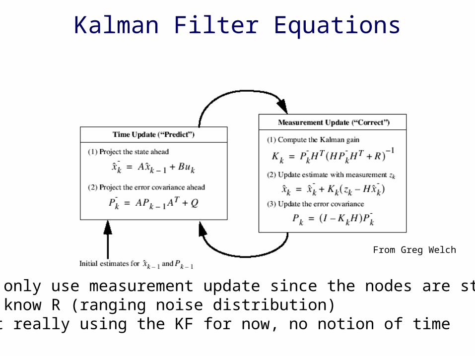
Kalman Filter Equations

From Greg Welch

• We only use measurement update since the nodes are static• We know R (ranging noise distribution)• Not really using the KF for now, no notion of time

Global Kalman Filter

Matrices grow with density and number of nodes => so does computation cost

Computation is not feasible on small processors with limited computation and memory

00)5(ˆ)5(ˆ

00)4(ˆ)4(ˆ

)3(ˆ)3(ˆ)3(ˆ)3(ˆ

00)2(ˆ)2(ˆ

)1(ˆ)1(ˆ00

5454

44

34344343

5353

3232

kk

kk

kkkk

kk

kk

z

yey

z

xexz

yey

z

xexz

eyey

z

exex

z

eyey

z

exexz

yey

z

xexz

eyy

z

exx

H # of edges

# of unknown nodes x 2

254

254

214

214

243

243

253

253

232

232

)()(

)()(

)()(

)()(

)()(

ˆ

yeyxex

yeyxex

eyeyexex

yeyxex

eyyexx

z Tk

Kalman Filter Equations

From Greg Welch

http://www.cs.unc.edu/~welch/media/pdf/kalman_intro.pdf

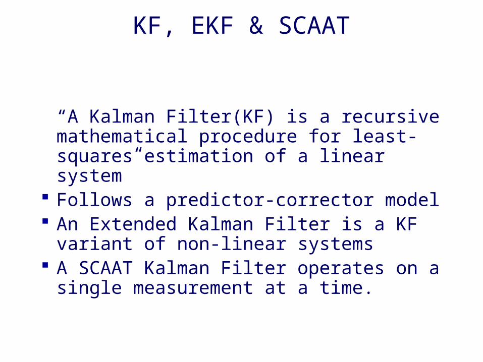
KF, EKF & SCAAT

“A Kalman Filter(KF) is a recursive mathematical procedure for least-squares estimation of a linear system”

Follows a predictor-corrector model An Extended Kalman Filter is a KF variant

of non-linear systems A SCAAT Kalman Filter operates on a

single measurement at a time.

SCAAT Kalman Filter

Proposed by Greg Welsh and Gary Bishop at UNC in 1997

Used in Hi-Ball Optoelectronic Tracker System

[Slide created from Welsh & Bishop, “SCAAT: Incremental Tracking with Incomplete Information”, Sigraph 97]

SCAAT Kalman Filter

Single-constraint-at-a-time(SCAAT)

• Process one measurement at a time

C- # of independent constraints for a unique solution

N – # of constraints used to derive an estimate

Nind - # of independent constraints

[Slide from Welsh & Bishop, “SCAAT: Incremental Tracking with Incomplete Information”, Sigraph 97]

SCAAT Aims at Temporal Improvements

Computation is faster KF matrices H, x and z are smaller The state prediction model described by

matrix A needs to change

Example system that uses all measurements at once

Beware of Solution Uniqueness Requirements

In a 2D scenario a network is uniquely localizable if:1. It belongs to a subgraph that is redundantly rigid

2. The subgraph is 3-connected

3. It contains at least 3 beacons

More details in future lectures

Nodes can be exchanged without violating the measurement constraints!!!

[conditions from Goldenberg04]

Does this solve the problem?

No! Several other challenges Solution depends on

• Problem setupo Infrastructure assisted (beacons), fully ad-hoc & beaconless, hybrid

• Measurement technologyo Distances vs. angles, acoustic vs. rf, connectivity based, proximity basedo The underlying measurement error distribution changes with each technology

The algorithm will also change• Fully distributed computation or centralized• How big is the network and what networking support do you have to solve

the problem?• Mobile vs. static scenarios• Many other possibilities and many different approaches

More next time…

Fundamental Behaviors and Trends

What is the fundamental error behavior?Measurement technology perspective

• Acoustic vs. RF ToF (2cm – 1.5m measurement accuracy)

• Distances vs. Angules

Deployment - what density?Scalability How does error propagate?Beacon density & beacon position uncertaintyIntrinsic vs. Extrinsic Error Component

Estimated Location Error Decomposition

PositionError

ChannelEffects

ComputationError

SetupError

Induced by intrinsic measurement error

Cramer Rao Bound Analysis

Cramer-Rao Bound Analysis on carefully controlled scenarios• Classical result from statistics that gives a lower bound

on the error covariance matrix of an unbiased estimate

Assuming White Gaussian Measurement Error Related work

• N. Patwari et. al, “Relative Location Estimation in Wireless Sensor Networks”

Density Effects

0 0.05 0.1 0.15 0.2 0.25 0.3 0.35 0.410

-1

100

101

102

angle measurementsdistance measurements

Density (node/m2)

RM

S L

ocat

ion

Err

or

20mm distance measurement certainty == 0.27 angular certainty

100

101

102

103

10-1

100

101

102

103

104

distancesangles

Range Error Scaling Factor

RM

S L

ocat

i on

Err

or/s

igm

a

Range Tangential Error

Results from Cramer-Rao Bound Simulations based on White Gaussian Error

m/rad

m/m

Density Effects with Different Ranging Technologies

0 0.1 0.2 0.3 0.4 0.5 0.6 0.7 0.80

0.1

0.2

0.3

0.4

0.5

0.6

0.7

0.8

Ranging Error Variance(m)

D=0.030D=0.035D=0.040D=0.045D=0.050D=0.055

RMS Error(m)

6 neighbors

12 neighbors

Network Scalability

x-coordinate(m) y-coordinate(m)

RM

S L

o cat

ion

Err

or x

10

Error propagation on a hexagon scenario (angle measurement)Rate of error propagation faster with distance measurements but Much smaller magnitude than angles

More Observations on Network Scalability…

Performance degrades gracefully as the number of unknown nodes increases.

Increasing the number of beacon nodes does not make a significant improvement

Error in beacons results in an overall translation of the network

Error due to geometry is the major component in propagated error