intra-asean trade gravity model and spatial hausman-taylor

source: https://doi.org/10.7892/boris.108786 | downloaded: 26.3.2022

1

Working Paper No. 20/2017 | December 2017

Intra-ASEAN trade – Gravity model

and Spatial Hausman-Taylor approach

Phung Duy Quang Foreign Trade University (FTU), Vietnam [email protected] Pham Anh Tuan Vietnam Military Medical University Nguyen Thi Xuan Thu Diplomatic Academy of Vietnam Abstract: This study examines determinants of intra-industry trade between Vietnam and Asean countries. By solving

endogenous problem and applying Hausman-Taylor model for panel two-way dataset, we detect that export flows of

Vietnam gravitate to neighbouring countries and those with similar GDP. More importantly, the research indicates the

existence of spatial-lag interaction.

Keywords: Intra-trade, export, import, gravity model, two-dimensions fixed effect panel model, Hausman-

Taylor model, Spatial Hausman - Taylor model.

Research for this paper was funded by the Swiss State Secretariat for Economic Affairs under the SECO / WTI Academic

Cooperation Project, based at the World Trade Institute of the University of Bern, Switzerland.

SECO working papers are preliminary documents posted on the WTI website (www.wti.org) and widely circulated to

stimulate discussion and critical comment. These papers have not been formally edited. Citations should refer to a

“SECO / WTI Academic Cooperation Project” paper with appropriate reference made to the author(s).

mailto:[email protected]

2

ACKNOWLEDGMENTS

From my heart, I would like to show my gratitude and sincere thanks to Dr. Anirudh

([email protected]), from World Trade Institute, Switzerland, who is my

mentor, for guiding me to find out research, practical approach, looking for material,

processing and data analysis, solving problem ... so that I can complete my research.

Also, in the process of learning, researching and implementing the research I was

getting a lot of attention, suggestions, supporting from my precious colleagues,

expertise and organizations. I would like to express deep gratitude to: SECO and FTU

which supporting finances to complete the research.

All members of my wonderful research team: Mr. Pham Anh Tuan, Dr. Nguyen Thi

Xuan Thu.

We sincerely thank Prof. Nguyen Khac Minh for giving us valuable comments and

advices.

3

Tables and Figure Page

Table 1. Lntrade by ASEAN countries 25

Figure 1. Share of Intra-ASEAN on ASEAN trade 27

Table 2. Share of Intra-ASEAN by ASEAN countries 28

Table 3. SIM and RLF by ASEAN countries 29

Table 4. Results of models concerning spatial effects and time effects 30

Table 5. Estimation results of HT Model and Spatial Hausman-Taylor

model

32

4

Intra-ASEAN trade – Gravity model and

Spatial Hausman-Taylor approach

Phung Duy Quang

Foreign Trade University (FTU), Vietnam

Email: [email protected]

Pham Anh Tuan

Vietnam Military Medical University


Nguyen Thi Xuan Thu

Diplomatic Academy of Vietnam


CHAPER 1. INTRODUCTION

In the 1930s, Eli Heckscher and Bertil Ohlin introduce the model of

international trade based on the theory of Ricardo. This model focuses on

differences in production factors such as labor and capital between countries

which are sources of international trade. In other words, countries tend to

manufacture and export commodities that the country has a comparative

advantage and might produce at a much lower opportunity cost (Eli F. Heckscher

& Bertil Ohlin, 1933). However, the model could not explain the intra-industry

trade which has been more and more popular in the more developed international

trade. This fact is unexplained by the comparative advantage theory. Additionally,

the theory of comparative advantage is unable to explain the transition of Taiwan

or South Korea from developing countries to developed countries, from exporting

shoes and clothes to exporting cars and computers. In fact, intra-industry trade is

plausible as export and import might happen at the same time in the same

industry.

5

According to Frenstra and Taylor (2011), this phenomenon could be

explained through assumptions on economies of scale, in which the large-scale

production reduces production costs. Consumers’ interest in product diversity is

also a plausible explanation. There are two types of intra-industry trade, namely

horizontal intra-industry trade driven by product differentiation and vertical

intra-industry trade driven by international fragmentation of the production.

Accounting for approximately one-third of world trade (Reinert KA., 1993,

1994), intra-industry trade has become an important part of world trade.

Through participation in intra-industry trade, a country can simultaneously

reduce the number of types of self-produced products and increase the variety

of goods to consumers in the local market. In the mid-1980s, some emerging

economics such as China, Hong Kong, Indonesia, Malaysia, Philippines,

Singapore, South Korea, Taiwan and Thailand constituted over 20 percent of

intra-industry trade in East Asia (Helvin, 1994). As reported by Thrope, M and

Z. Zang (2005), since mid-1970s to mid-1990s, intra-industry trade increased

to about 50 percent from 25 percent. For the period from 1981 to 2001, intra-

regional trade increased 3.1 times and 6.7 times in the world and East Asia

respectively. This might reflect an increasingly important role of intra-industry

trade in the international trade (Mitsuyo Ando, 2006).

In the past few decades, since the implementation of DoiMoi program in

1986, the Vietnamese Government has pursued a policy of liberalization and

market-oriented pricing, better exchange rate management, modernized financial

systems, tax reform and fair competition between private enterprises and

monopoly state-owned enterprises. Consequently, Vietnam's economy has

achieved high GDP growth, macroeconomic stability, trade promotion,

investment and poverty reduction. The economic achievements of Vietnam in the

last decade have been impressive, thanks to the policy of trade liberalization

associated with international economic integration. Vietnam became a member

of the Association of Southeast Asian Nations (ASEAN) in 1995, and joined the

6

World Trade Organization (WTO) in 2007. ASEAN has always been a strategic

trading partner of Vietnam since 1995. Particularly, the annual growth rate of

bilateral trade between Vietnam and ASEAN was about 12.3% during the period

1996 – 2006 and 8.1% for the period 2007 – 2016 (Vietnam Customs 2017). The

bilateral trade between Vietnam and ASEAN countries would be even more

strengthened with the establishment of ASEAN Economic Community (AEC)

on 31.12.2015. This community brings ASEAN into a single market and

production base; an equal regional development; competitive economic sector

and strong integration into the global economy. Vietnam has actively

participated in the integration of AEC activities, especially activities aimed at

liberalizing trade in goods and services. Although Vietnam is not at the level of

high development compared to some countries in the region, according to the

grading of ASEAN, over the period of 2008 through 2013, Vietnam is one of

three best countries, which fulfill the commitments in the AEC Blueprint. AEC

is expected to bring about both opportunities and challenges because Vietnam

has to totally cut import taxes imposed on goods bought from ASEAN countries

to zero by 2018. Therefore, Vietnam should take advantages of this opportunity

for its economic development. This fact has motivated us to shed the light on

determinants of intra-industry trade flows between Vietnam and ASEAN

countries in recent years. Particularly, the objectives of this research are: (i)

Explore determinants of intra-industry trade flows between Vietnam and

ASEAN countries in recent years; (ii) Draw implications on how Vietnam could

integrate more effectively and take advantages of joining ASEAN in the

perspective of trade; (iii) Evaluate spillover from the economic growth of

ASEAN countries to exports of Viet Nam.

In order to do so, we apply Gravity model and Spatial Hausman-Taylor

approach. Different from other intra-trade studies using the Hausman Taylor

spatial model, the purpose of this research is to estimate time-invariant variables

and spillovers between ASEAN countries.

7

CHAPER 2. BACK GROUND OF THE RESEARCH

AND METHODOLOGY

2.1. Background of the research

In the last decade, Vietnam has actively integrated into the world market,

which was evidenced by its WTO membership and its conclusion of some

regional and bilateral free trade agreements (FTA). Among them, the ASEAN

Free Trade Agreement (AFTA) is the most important regional FTA. To analyze

the impacts of various factors on internal trade in the sectors between Vietnam

and other ASEAN member countries, we used the gravity model. This model

was initiated by Tinbergen (1962) and Poyhonen (1963) and widely applied in

experimental studies to quantify commercial impact of the economic linkages

bloc. They concluded that exports are positively affected by the income of the

trading countries and that distance can be expected to negatively affect to

exports. In the later years, in 1979, Anderson applied product differentiation

referred to the Armington Assumption which implied that there is imperfect

substitutability between imports and domestic goods, based on the country of

origin. He assumed Cobb-Douglas preferences and these products differentiated

by country of origin. Gravity model of international trade flows has been widely

used as a base model to calculate the impact of a range of policy issues relating

to regional trade groups, monetary union and various trade distortions.

In Vietnam, there have been many studies using gravity models to assess

the impact of FTAs that Vietnam participated. Thai (2006) analyzed trade

between Vietnam and 23 countries in Europe (EC23) through gravity model

and panel data. Variables included in the model are GDP of Vietnam and

partner countries, population, exchange rates, geographical distance and

history dummy. Tu Thuy Anh and Dao Nguyen Thang (2008) evaluated the

factors affecting the level of integration of Vietnam trade between ASEAN +3

countries. The model deployed in the study included three groups of factors

that affect trade flow, including the group of factors affecting supply (GDP and

8

population of the exporting country), the group of factors affecting demand

(GDP and population importing country) and the group of attractive factors or

prevention (geographical distance). Nguyen Anh Thu (2012) used a gravity

model to examine the impact of the economic integration of Vietnam under the

ASEAN Free Trade Agreement (AFTA) and the Economic Partnership

Agreement Vietnam-Japan (VJEPA) on Vietnam's trade. The dependent

variables in the model are GDP, the gap between countries, per capita income,

the real exchange rate and the dummy variables VJEPA, AFTA, AKFTA.

The gravity model has achieved undeniable success in explaining the

types of international and inter-regional flows, including international trade in

general and intra-industry trade in particular by applying varying types such

migration, foreign direct investment and more specifically to international trade

flows. Prediction of gravity model researches about bilateral trade flows

depends on the economy scale and the gap between countries. According to this

model, exports from country i to country j are explained by their economic sizes

(GDP or GNP), their populations, direct geographical distances and a set of

dummies incorporating some kind of institutional characteristics common to

specific flows.

In order to examine the impact of every country, we deploy the panel

data. In particular, Matyas (1997) designated an economic model so called

“triple-way model” in which impacts of time, export and import countries are

fixed and unobserved. However, Egger and Pfaffermayr (2002) prove that when

the “triple-way” model is extended to include bilateral trading impacts, “three-

way” should simply become “two-way” model with impacts of time and

bilateral trade. Even though estimation techniques in panel data like Pooled

OLS, Fixed Effect models, or Random Effect models have been applied widely,

assumptions in which unobservable effects are correlated to regressors have

been neglected in many researches. This makes research results biased.

Therefore, Fixed Effect estimates are commonly used to limit the bias of

9

estimations. However, it should be noted that Fixed Effects are not used to

estimate time-constant variables like the distance. In order to meet this

objective, we apply Hausman-Taylor Estimation in Heterogeneous Panels.

Our main empirical findings are summarized below. First, the impact of

the GDP variables is always significantly positive, whereas the impact of

population variables is found to be mostly insignificant. Second, the impact of

the distance variable is always significantly negative. Third, the impact of

similarity in relative size of trading countries is mostly significant and positive,

while the impact of differences in relative factor endowments (RLF) is

somewhat ambiguous. A distance variable is commonly used to estimate spatial

relations (like geographical location, language, or free trade agreements…).

However, this variable is unable to explain interactions amongst neighboring

countries which might lead to spatial spillover effects. Therefore regarding HT

estimation, there is a spatial interaction between spatial states.

2.2. Methodology

2.2.1. Grubel and Lloyd index (GL Index)

Grubel and Lloyd index (GL Index) (Grubel and Lloyd) is enormously

popular for analysis of intra-industry trade. This index is considered the most

appropriate evaluation of commercial structure in a specific period. It is

calculated by the following formula:

n n

ijk ijk ijk ijki 1 i 1

njk

ijk ijki 1

(X M ) X M

IIT

(X M )

(1)

where: IIT is intra-industry index; i

X is export and i

M is import; i denotes

commercial good; j and k are export and import countries respectively; n is the

number of traded commodities of two countries with each other.

10

IIT index has a value between 0 and 1, IIT equal 0 means that the trade

between countries j and k is completely inter-industry trade; if the value is 1

trade between countries j and k is completely intra-industry trade. If IIT value is

≥ 0.5, trade between countries j and k mainly due to intra-industry trade.

Otherwise, IIT <0.5 is mainly due to the impact of inter-industry trade.

2.2.2. Gravity model

Gravity model is an effective tool to formulize the volume and direction

of bilateral trade between countries and widely used in international trade

(Matyas 1997). The key assumption of this model, which is the commercial

activities, complies with Newton's theory of gravity. Particularly, the intensity of

trade between two countries is positively related to the size and inversely related

to the geographical distance of the two countries. Standard equation is:

ij i j ijX G.(M M / D ) (2)

Where: ij

X is trade flow between countries i and j, M represents

measured volume (size), D is a distance between countries (or economic

centers) and G is a constant.

It has become widely recognized that Gravity model has a number of

advantages compared with other models because of the following reasons: (i)

relative easiness in finding data, (ii) a transparent and simple function, thus makes

sense in economic terms, (iii) the fact of the event and (iv) the ability to highly

interpret and assess the impact of various factors separately for international trade,

which may separate the effects of the free trade agreement (FTA).

However, there are some limitations associated with the use of a

standard gravity model, including: (i) the sustainability of the economic

functional form of model is a question mark, (ii) there may exist an

endogenous relationship between changes in trade flows and the formation of

the agreement (increasing trade leads to the formation of the agreement rather

11

than the opposite. Hausman and Taylor (1981) suggest an IV estimator for this

endogenous problem, so it could be solved through causality test or Hausman-

Taylor estimation.

Bilateral exports and imports are defined as logarithms of export R

hftX and

import R

hftM :

R N

hft hft

US

100X X

XPI and R N

hft hft

US

100M M

MPI (3)

where N

hftX and

N

hftM are bilateral export and import measured in millions of US

dollars, US

XPI and US

MPI are the US export and import price indices.

Then, the total volume of trade is given by:

R R

hft hftlnTrade ln(X M ) (4)

GDP of country h (home country) and country f (foreign country) are defined as

logarithms of R

htGDP and

R

ftGDP .

Furthermore, the standard gravity model is augmented with a number of

variables to test whether they are relevant in explaining trade. These variables

are specified in three dimensions. Firstly, the basic model specifies that or

trade depends on the variable measured by GDP and population of home and

foreign countries. Barrier to trade is measured by distance. Secondly, we

consider the augmented specification, where trade flows are also allowed to

depend on variables that take into account free trade agreements as well as

dummy for common border. Finally, due to recent developments of the New

Trade Theory advanced by Helpman (1987), Hummels and Levinsohn (1995)

and Egger (2001, 2002), we thus add variables such as RLF and SIM. The

difference in terms of relative factor endowments proxied by per capita GDPs

between two countries is measured by the variable RLF and when there is

equality in relative factor endowments, it takes a minimum value of zero. The

12

larger is this difference, the higher is the volume of inter-industry which leads

to the total trade will be, and the lower the share of the intra-industry trade.

R R

it ft htRLF ln PGDP PGDP (5)

The relative size of two countries in terms of GDP is captured by the

variable SIM. The value is bounded between zero which is absolute divergence

in size and 0.5 which is equal country size. The larger this index is (meaning

that the more similar two countries are), the higher the share of the intra-industry

trade will be.

2 2R R

ht ft

it R R R R

ht ft ft ht

GDP GDPSIM 1

GDP GDP GDP GDP

(6)

Real exchange rate in constant dollars at 2010 are defined as

it it USRER NER XPI , where

itNER is nominal exchange rate between

currencies h and f in year t in terms of dollars.

2.2.3. The Hausman-Taylor Panel Data Model

Gravity models have been very successful in interpreting flow factors,

such as migration or traffic flow. For the international trade flows, the

gravity model shows that the scale of bilateral trade flows are determined by

the supply conditions of the export country, the demand conditions of import

country, and other effects to the trade flow. After the study of Anderson

(1979), some studies have found that the gravity model might be derived from

different structures, such as the Ricardian model, the Hecksher-Olin model,

increasing returns to scale model of modern trade theory.

Although the gravity model does not evaluate the validity of trade

theories, the experimental success of the model is derived from the ability to

combine the phenomena experienced in the global trade. Almost all previous

studies used OLS with cross-sectional data. However, OLS estimations with

13

cross-sectional data do not consider a non-homogenous characteristic related to

the bilateral trade. For example, a country might export different volume of a

product to two different countries even though GDP of these two import

countries is similar. Therefore, OLS might lead to the bias of estimations. It is

reasonable that the panel data has been used more widely in recent researches

because it covers issues related of non-homogeneity. However, in the trade

flow studies, distance amongst countries play an important role. In the previous

researches, geographical distance, which is commonly used to examine the

impacts of distance on export countries, is unable to present the spillover

between neighboring countries. For instance, a country might export different

volumes of the same product to different countries at different distances.

However, these geographical distances might have impacts on the export

volumes. Therefore, spatial spillovers play a crucial role in studies on the trade

flow.

Our research explores the determinants of intra-industry trade flows

between Vietnam and ASEAN countries in recent years and draws some

implications on how Vietnam could integrate more effectively as well as take

advantage of being an ASEAN member in the field of trade. A gravity model of

international trade is empirically tested to investigate the relationship between

the volume and direction of international trade and the formation of regional

trade blocs where members are in different stages of development.

We apply our proposed Hausman Taylor (HT) estimation technique

along with the conventional panel data approaches. There are some additional

advantages of using the panel data rather than cross-sectional data or time series

data. Besides handling both changing issues across the country at a time (cross-

sectional) and changes over time, panel data can allow us to control impact of

heterogeneity (abnormal movements which are consistent, but are not observed

and measured among the economies over time). The fixed effects (represented by

14

such variables as the constant distance between all exporters/importers) can be

estimated directly, as opposed to the random effects (variables with specific

distribution function), usually based on a strong assumption that the unobserved

effects do not correlate with the observed effects. Another advantage of HT is to

avoid the potential bias of the uncorrected estimates.

This extended panel data setup generalizes HT estimation, develops the

underlying econometric theory, and proposes an alternative source of

instruments in addition to the (internal) instruments suggested by HT; namely,

some of (consistently estimated) heterogeneous time-specific factors under the

assumption that they are correlated with individual specific variables but not

with unobserved individual effects.

We begin with panel data model with two-way fixed effects as follows:

hft hf t 1 hft 2 ht 3 ft 4 ht hfty x x x z u (7)

Where h,f 1,2,...,N, h f , t 1,2,...,T ; hft

y is the dependent variables

(the volume of trade from home country h to target country f at time t); hft

x are

explanatory variables with variation in all the three dimensions; ht ft

x , x are

explanatory variables with variation in h or f at t (GDP, population); hf

z are

explanatory variables that do not vary over time but vary in h and f (distance);

hf is an individual effect that might be correlated with some or all of the

explanatory variables; t

are time-specific effects common to all cross-section

units that are meant to correct for the impact of all the individual invariant

determinant such as potential trend or business cycle.

Fixed effects model is not able to estimate the coefficients on time-

variant variables such as distance. Thus we now consider the following more

conventional double index panel data model:

it it i ity x z ,i 1,...,N;t 1,2,...,T (8)

15

it i t itu

Where it 1,it k ,itx x ,...,x

is a k 1 vector of variables that vary over

individuals and time periods, i 1,i g,iz z ,...,z

is a g 1 vector of time- invariant

variables. There are three components in the error term it ; namely,

i refers to

effects of all possible time invariant determinants and might be correlated with

some of the explanatory variables it

x and i

z ; t

is the time-specific effects

common to all cross section units that is meant to correct for the impact of all the

individual invariant determinants such as potential trend and business cycle; and it

u

is a zero mean idiosyncratic random disturbance uncorrelated across cross section

units and over time periods. We assume that these three components are unrelated

to each other.

From the research model HT designate attractive model as follows:

R R R R

ft ht ft ht it it

ht ft

lnTrade lnGDP lnGDP ln POP ln POP SIM RLF

RER RER ln DIST

(9)

2.2.4. Spatial Hausman-Taylor Panel Data Model

Baltagi et al (2016) introduces spatial spillovers in total factor productivity

by allowing the error term across firms to be spatially interdependent. In order to

make allowance for spatial correlation in the error term, this model is estimated by

extending the Hausman-Taylor estimator. Baltagi also found an evidence of

positive spillovers across firms and a large and significant detrimental effect of

public ownership on total factor productivity. This economic problem is solved

through several spatial econometric models. Firstly, Spatial Autoregressive model

(SAR) is proposed when we review the spatial dependence as long run equilibrium

of an underlying spatio-temporal process. In the cases of economic shocks or

spatial dependence of omitted variables, we might use the Spatial error model

16

(SEM). However, regarding fixed-effects, these two models are unable to estimate

time-invariant variables. We will refer to the spatial Hausman-Taylor model to

solve our model in case of spatial correlation between regions or countries.

In recent years, there is a trend to estimate econometric relationships

using spatial panels which typically refer to time series data of observations of a

number of spatial units (zip codes, municipalities, regions, states, etc.). In this

section we provide a review and organize these methodologies. It deals with the

possibility to test for spatial interaction effects in standard panel data models,

the estimation of fixed effects, the possibility to test the fixed effects

specification of panel data models extended to include spatial error

autocorrelation and a spatially lagged dependent variable.

Spatial effects

Starting to study about the impact of space, we will consider a simple

panel data linear regression model as follows:

it it ity x (10)

Where i is an index about the dimension of cross data with i 1,2,...,N , t

is an index about the dimension of time with t 1,2,...,T . it

y is an observation on

the dependent variable at i and t, it

x a 1 K vector of observation on the

(exogenous) explanatory variable, a matching K 1 vector of regression

coefficients, and it an error term.

Given our interest in spatial effects, the observations will be stacked as

successive cross-sections for t 1,2,...,T and notate as t t t

y ,X , . Then panel

data regression model is written as follows:

y X (11)

where y as a NT 1 vector, X as a NT K matrix and as a NT 1 vector.

17

In general, spatial dependence is considered when the correlation across

cross-section units is non-zero, and the pattern of non-zero correlations follows a

certain spatial ordering. When the appropriate spatial ordering is known a little,

the spatial dependence is reduced from dependence of cross-section data. For

example, the error components is spatial correlation when it jt

E 0 with each

t and i j , and the non-zero covariance conform to a specified neighbor relation.

The neighbor relation is expressed by means of a so-called spatial weights matrix.

We mentioned the concept of weights matrix, in this section, we will outline the

detail of the two classes of specifications for model with spatial dependence. First,

the spatial correlation pertains to the dependent variable in a so-called spatial lag

model, in the other it affects the error terms, a so-called spatial error model.

Weights matrix

To studythe convergence across space, we have to build models and test

whether the spatial dependence exists. In order to do so, it is necessary to build a

weight matrix and implement the necessary testing.

Our proposed spatial econometric model uses countries as the spatial

units. The method to identify a weight matrix is as follows: For each country, we

identify a central point (the capital). We can identify the latitude and longitude

of this central point by using a geographical map. Using the Euclidian distance

in the two-dimension space, we have:

T

ij i j i j i jd d s ,s s s s s (12)

Two countries are called neighbors if *

ij0 d d , *d is the critical cutting

point. We also define two countries called neighbors if ij ikd min d , i,k . Put

N i is the set of all neighbors with country i, then the weighted matrix

ij N NW w

is determined as follows:

18

ij

1 if j N iw

0 otherwise

(13)

Denote ij*

j ij ij

j

ww , w

n , then * *

ij N NW w

is called a row-

standardized binary version of a spatial weight matrix. Using this methodology,

we can construct the weight matrix for the intra-trade gravity model of Asean.

Type of spatial weights matrix is very important for spatial econometric

applications. Unless, the weights based on an official theoretical model for

society or spatial interaction. In the empirical, we can choose according to

geographical criteria as binary. In the empirical research, we can choose

according to geographical criterias as contiguity (sharing common boundaries)

or distance, including nearest neighboring distance (Anselin, 1988a, Chapter 3).

Combining generalization about the concepts of "economic" distance is

increasingly being used regularly (Case et al, 1993; Conley and Ligon, 2002;

Conley and Toga, 2002). A different kind of economic weights called weight

block, where the observations of the same region are considered neighboring.

If g

N the number of units in the block (such as districts in the province), all are

considered as neighboring and spatial weight equal to g1/ N 1 for all

observations in the same block (Lee, 2002).

In addition, weight is examined in tamed cross data. We will expand the

use of panel data which are assumed to be constant by the time. Notation N

W is

the spatial weight matrix for cross data and the number of observations given in

the model (11), so the matrix for panel datais defined as:

NT T NW I W

withT

I as an identity matrix of dimension T.

19

Unlike the case of time-series, "neighboring" observations are combined

directly into the model through the operator above (means t-1), which it was not

clear in establishing two-way space. For example, observing the irregular spatial

units, such as surveyed districts or regions, often does not have the same number

of neighbor, so the spatial operator above can not be done. Also, in spatial

econometric, the neighbor observations included through the operator is called

spatial lag, like a lag distribution rather than a change (Anselin, 1988a). In

essence, a spatial lag operator creates a new variable contains weighted average

of neighbor observations, with the weight here is W . Normally, if observation i

of cross data is variable z, the spatial lag will be ij j

j

w z . In most applications,

the large number of elements of the row is equal to 0 so the impact on the total

of j is just the combination of the "neighbor" ones.

Spatial variables specified in the model are applied spatial lag operator of

the dependent variables and to become the explanatory variables or error

components. A variety of models for local spatial elements or the entire can be

appointed in the manner above (Anselin, 2003). This expansion is set in the

panel data by weighted matrix with level NT NT associated with y,X, from

the model (10). More specifically, we will denote as follows:

NT T NWy W y I W y

NT T NWX W X I W X

NT T NW W I W

Spatial Hausman-Taylor model

In this section, we will revisit Hausman-Taylor models with spatial

correlation suggested by Baltagi et al.(2011). The spatial model for time t is given

by:

20

t t t t ty X Z u A u (14)

t t tu Wu ,

t t

Where t tA X ,Z and , . The explanation variable can be

decomposed (decomposed) into t U CtX X ,X and U C

Z Z ,Z , where subindex

C denotes regressors which are correlated with while subindex U indicates

regressors which are uncorrelated with . W is an N N observed non-

stochastic spatial weights matrix; 2

i~ IID 0;

and time-invariant

2

it~ IID 0,

.

Aggregated model for all periods as below:

Ty X Z u A u (15)

Tu I W u ,

Z

Where T N

Z I is an NT N selector matrix of ones and zeroes.

For estimation, we employ moment conditions derived in Kapoor et al

(2007) for the SRE model and Baltagi et al (2016). In which, need to note the

following assumptions:

Assumption. (Instrument set HT

H )

(i) The instrument are uncorrelated with the error .

(ii) The matrix HT 0 1 U T UH Q X,Q X , Z , in which 1

1 T T NQ T I

and 0 NT 1

Q I Q has full column rank.

(iii) The elements of HT

H are uniform bounded in absolute value.

21

(iv) 1

I INlim NT H H

exist, is finite and nonsingular.

(v) 1

IN

plim NT H Z

exist, is finite and has full column rank.

Testing for specification SFE, SRE and SHT

For the specification test of FE, RE or HT we use the spatial Hausman test

proposed by Mutl and Pfaffermayr (2011):

SH SRE SFE SFE SRE SRE SFEˆ ˆ ˆ ˆ ˆ ˆm var var

Where superscript “-” refers to the generalized inverse, SH

m is distributed

as 2

SFE SREˆ ˆrank var var

under the null hypothesis of no correlation

between A and . If the null is rejected, the SRE is not consistent.

We also use the Hausman test to choose between SHT and

SFE which is

given as follows:

SHT SHT SFE SFE SHT SHT SFEˆ ˆ ˆ ˆ ˆ ˆm var var

And is distributed as 2

U CK R .

Testing for spatial dependence

Moran’I index:

Statistical test:

T

T

e WeI

e e

where: e is residual vector, W is spatial weight matrix. With an assumption that

residuals follow normal rules, I-Moran statistic will approach the normal

distributions with:

22

k 1

E I tr MWN k 1

2T 2

2tr MW MW tr MW tr MW

V I E IN k 1 N k 1

where tr is the trace of an matrix, 1

T TM I X X X X

.

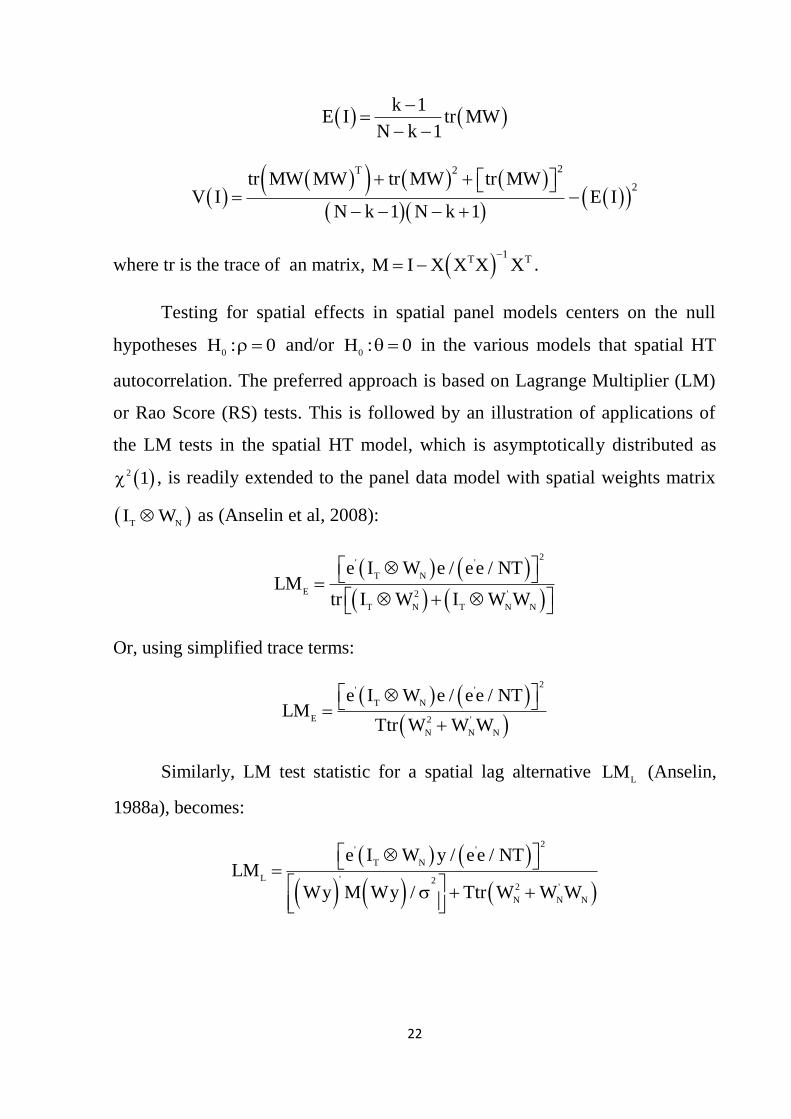
Testing for spatial effects in spatial panel models centers on the null

hypotheses 0

H : 0 and/or 0

H : 0 in the various models that spatial HT

autocorrelation. The preferred approach is based on Lagrange Multiplier (LM)

or Rao Score (RS) tests. This is followed by an illustration of applications of

the LM tests in the spatial HT model, which is asymptotically distributed as

2 1 , is readily extended to the panel data model with spatial weights matrix

T NI W as (Anselin et al, 2008):

2' '

T N

E 2 '

T N T N N

e I W e / ee / NTLM

tr I W I W W

Or, using simplified trace terms:

2' '

T N

E 2 '

N N N

e I W e / ee / NTLM

Ttr W W W

Similarly, LM test statistic for a spatial lag alternative L

LM (Anselin,

1988a), becomes:

2' '

T N

L ' 22 '

N N N

e I W y / ee / NTLM

Wy M Wy / Ttr W W W

23

with T NWy I W X as the spatially lagged predicted values in the

regression, and 1

' '

NTM I X X X X

. This statistic is also asymptotically

distributed as 2 1 .

2.2. 5. Empirical Application to the Intra-ASEAN Trade

2.2.5.1 Explanatory Data Analysis

The export and import data of Vietnam are based on data from Ministry of

Industry and Trade for 11 continous years from 2004 to 2015. The data covers

trading information (export and import) of product from all business sectors

between Vietnam and countries in ASEAN region including Brunei, Cambodia,

Indonesia, Lao PRD, Malaysia, Myanmar, Philippines, Singapore, and Thailand.

The gross domestic product (GDP) and population of home and countries of

destination are obtained from World Bank database. GDP deflator index is from

World Bank World Development Indicators and IMF data source. GDP per capita

and nominal exchange rates are from the World Bank World Development

Indicators. Data on the distance between the capital of Vietnam (Hanoi) and the

capital of import countries is used to capture the distance from Vietnam to different

countries; all distances are indicated according kilometers in the form of logarithm.

This data is from the website Prokerala.com.

The gravity model uses distance to model transport costs which is not only a

function of distance but also of public infrastructure. We use Liner shipping

connectivity index since 2004 (maximum value in 2004 = 100) to capture how well

countries are connected to global shipping networks. It is computed by the United

Nations Conference on Trade and Development (UNCTAD) based on five

components of the maritime transport sector: number of ships, their container-

24

carrying capacity, maximum vessel size, number of services, and number of

companies that deploy container ships in a country's ports. The import and export

price index of United States are collected from Federal Reserve Bank of St. Louis.

Table 1. Lntrade by ASEAN countries

Country

Lntrade

Average Std Min Max

Brunei 15.82287 1.138898 13.44579 16.97431

Cambodia 21.12426 0.603751 19.94215 21.88184

Indonesia 20.99428 0.565998 20.1188 21.72142

Lao PRD 19.14387 0.654676 18.20762 20.1062

Malaysia 21.5717 0.607231 20.4447 22.51727

Myanmar 17.91138 1.166513 16.47902 20.1212

Philippines 21.01103 0.352523 20.20371 21.39041

Singapore 21.58359 0.159089 21.31644 21.93355

Thailand 21.20318 0.522105 20.27488 22.04824

Source: Author’s estimation based on World Bank data

Table 1 below shows the log trade values. The table indicates that bilateral

trade flows in ASEAN are relatively equal. However, Brunei is an exception with

the log trade value is lower than other countries. It sounds reasonable because

compared to other ASEAN countries, Brunei is relatively small market with a

population of about 434000. Additionally, since Brunei has already established a

long-lasting trading relationships (like Thailand), it is more difficult for Vietnam to

export to Brunei (VCCI 2015). Interestingly, Myanmar has a growing trade flow.

25

This is in line with the fact that since being an ASEAN membership, Myanmar has

started to open its economy and as a result increased its trade flows rapidly in

recent years.

Figure 1. Share of Intra-ASEAN on ASEAN trade

Source: Author’s estimation

Figure 1 shows that the intra-ASEAN trade has always been a

considerable part of ASEAN’ s total trade. Although the share of intra-ASEAN

on ASEAN trade fluctuates within 12 years from 2004 to 2015, it still accounts

for nearly two-thirds total trade of ASEAN. Beginning at 65% on total trade in

2004, the share of intra-ASEAN declined dramatically in the following 5 years.

In 2010, the figure returned to original position, continually increased to 66% in

2012 before declining slightly to 59% in 2015 due to price increases in primary

goods.

In general, it can be seen that intra-industry trade in Vietnam and other

countries in Southeast Asia have gradually increased fluctuations, which reflects

monopolistic competition market and diversity in tastes of consumers about

export and import of products with similar quality.

26

In trading relations with Vietnam, Indonesia, Lao PRD and Malaysia are

the countries have the highest intra-industry trade share with an average of more

than 80% per year in the period 2004-2015, which followed by Singapore, the

Philippines, Myanmar ... and Brunei accounts for least share of intra-industry

trade with Vietnam.

Table 2. Share of Intra-ASEAN by ASEAN countries

Country 2004 2005 2006 2007 2008 2009 2010 2011 2012 2013 2014 2015

Brunei 0.463 0.476 0.471 0.487 0.657 0.698 0.826 0.151 0.054 0.056 0.052 0.051

Cambodia 0.508 0.448 0.357 0.33 0.245 0.298 0.3 0.495 0.293 0.294 0.31 0.311

Indonesia 0.811 0.802 0.972 0.92 0.606 0.683 0.857 0.976 0.976 0.983 0.953 0.947

Lao 0.958 0.83 0.726 0.683 0.73 0.807 0.813 0.768 0.973 0.813 0.828 0.814

Malaysia 0.678 0.9 0.917 0.81 0.878 0.819 0.76 0.829 0.863 0.909 0.961 0.92

Myanmar 0.84 0.415 0.407 0.448 0.602 0.729 0.65 0.986 0.963 0.703 0.484 0.358

Philippines 0.548 0.404 0.609 0.6 0.351 0.471 0.582 0.688 0.68 0.72 0.737 0.721

Singapore 0.582 0.599 0.448 0.453 0.45 0.457 0.682 0.503 0.523 0.636 0.604 0.617

Thailand 0.436 0.533 0.47 0.431 0.416 0.454 0.348 0.466 0.657 0.66 0.617 0.612


The values of SIM variable are more than 0 and towards 0.5. This

demonstrates that there is a positive correlation between the intra-industry trade

share and SIM. The values of RLF is relative high, it means that there has a clear

difference in terms of relative factor endowments proxied by per capita GDPs

between two countries. The larger is this difference, the higher is the volume of

inter-industry which leads to the total trade will be, and the lower the share of the

intra-industry trade.

In other words, we find a negative correlation between the intra-industry

trade share and RLF, and a positive correlation between the intra-industry trade

27

share and SIM. As Helpman (1987) indicated that it is interpreted as supporting

evidence of the theory of IRS and imperfect competition in international trades.

Table 3. SIM and RLF by ASEAN countries

Country

SIM RLF

Average Std Min Max Average Std Min Max

Brunei 0.177099 0.015109 0.158565 0.208854 10.32569 0.054479 10.22025 10.39971

Cambodia 0.168479 0.023971 0.137073 0.20529 6.25025 0.160973 6.051945 6.498219

Indonesia 0.256887 0.026136 0.209019 0.284011 7.476939 0.132354 7.276593 7.672846

Lao PRD 0.106839 0.032133 0.067464 0.15373 5.150435 0.128838 4.906211 5.30005

Malaysia 0.439538 0.024712 0.404713 0.470422 8.959761 0.095705 8.810333 9.126074

Myanmar 0.167406 0.179111 0.028007 0.461831 6.10325 0.341297 5.34471 6.67705

Philippines 0.462407 0.024438 0.428672 0.492345 6.721034 0.069706 6.629614 6.856646

Singapore 0.449659 0.029617 0.411953 0.487942 10.69156 0.098774 10.52253 10.82318

Thailand 0.389786 0.026732 0.351409 0.427372 8.210206 0.083843 8.067706 8.31635


2.2.5.2 Estimation results

The research considers both dimensions of panel data, namely country

and time dimensions. Firstly, in terms of country spatial one, we used a

Hausman test to decide whether FE or RE should be used. The observed value is

34.21 with statistically significant level at 0.000; therefore, FE will be deployed.

Column 2 of table 4 presents results of model concerning spatial

dimension. Variable lndist is constant over time so that it is removed from the

model. As can be seen in column 2, coefficients of variables Lnpoph, Sim, and

RERF are statistically significant. While the coefficient of lnpopvn is positive,

that of lnpopf is negative. It means that in ASEAN trade, population of

countries does not matter for export to them. More interestingly, populated

countries are not as attractive as those with less population. Additionally,

28

positive and significant coefficient of Sim indicates that countries with similar

GDP are more attractive to each other than those with different GDP.

Table 4. Results of models concerning spatial effects and time effects

Country effects Time effects

Variable Coefficient Variable Coefficient

LnGDPh -0.0573

(0.952) LnGDPh

1.1125

(0.753)

LnGDPf 0.1481

(0.151) LnGDPf

-0.89***

(0.000)

Lnpoph 24.931***

(0.000) Lnpoph

8.097

(0.478)

Lnpopf -8.7343***

(0.000) Lnpopf

2.074***

(0.000)

Sim 5.896***

(0.000) Sim

2.457*

(0.051)

RLF 0.2575

(0.277) RLF

0.516***

(0.003)

RERF 2.9755***

(0.000) RERF

5.27***

(0.001)

RERH 9233.5

(0.424) RERH

11423.64

(0.788)

LnDist LnDist -1.555

(0.000)

F-test 197.3

(0.000)

Hausman 34.21

(0.000) Hausman

0.23

(0.9998)


(p-value in parentheses *** p<0.01, ** p<0.05, * p<0.1)

Column 4 of table 4 shows results of model concerning time dimension.

Different from the model with spatial dimension, this model designates random

effects. Positive and significant coefficient of lnpopf indicates that over time

countries with large population are more attractive to export products than those

with less population. Especially, coefficient of lndist is negative and is

29

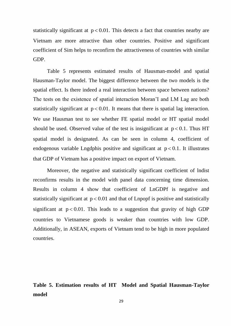
statistically significant at p 0.01 . This detects a fact that countries nearby are

Vietnam are more attractive than other countries. Positive and significant

coefficient of Sim helps to reconfirm the attractiveness of countries with similar

GDP.

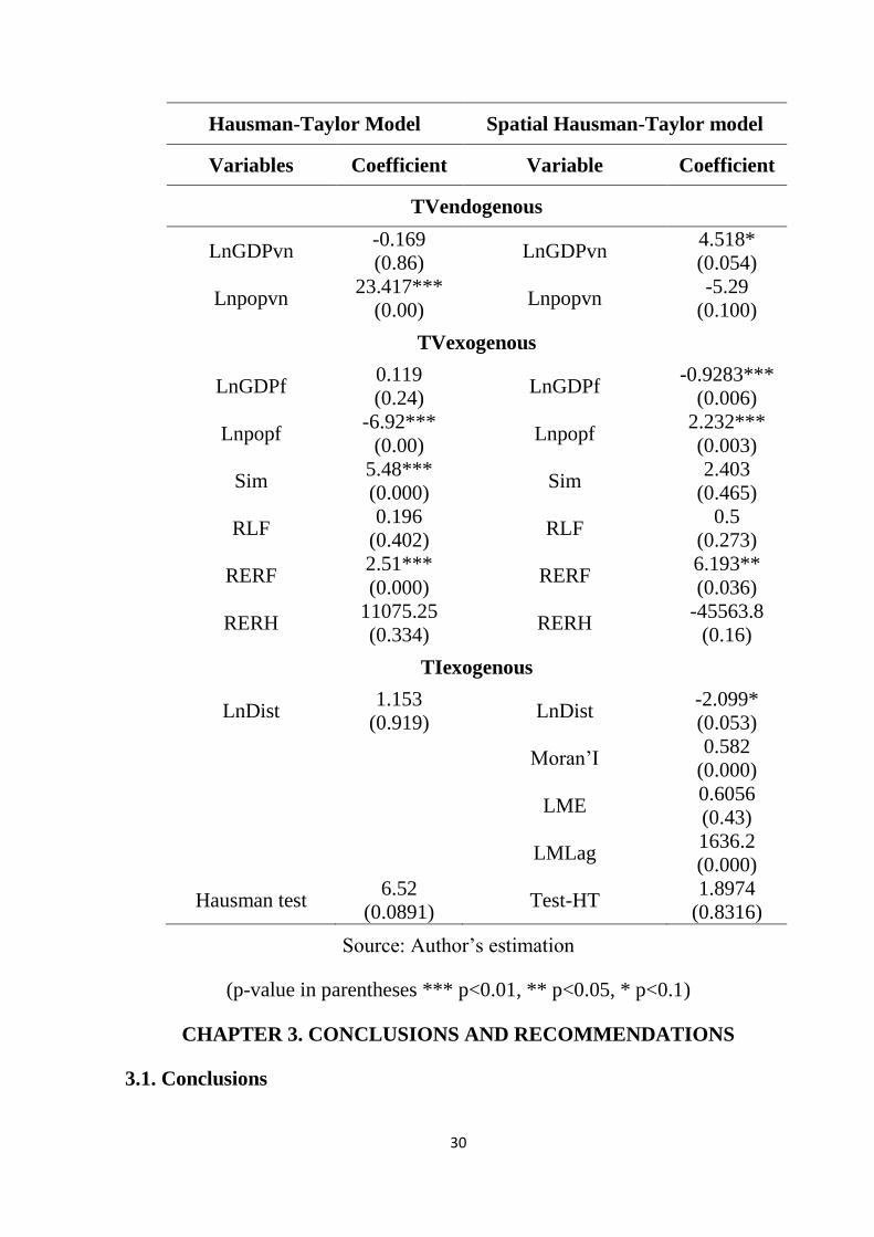
Table 5 represents estimated results of Hausman-model and spatial

Hausman-Taylor model. The biggest difference between the two models is the

spatial effect. Is there indeed a real interaction between space between nations?

The tests on the existence of spatial interaction Moran’I and LM Lag are both

statistically significant at p 0.01 . It means that there is spatial lag interaction.

We use Hausman test to see whether FE spatial model or HT spatial model

should be used. Observed value of the test is insignificant at p 0.1 . Thus HT

spatial model is designated. As can be seen in column 4, coefficient of

endogenous variable Lngdphis positive and significant at p 0.1 . It illustrates

that GDP of Vietnam has a positive impact on export of Vietnam.

Moreover, the negative and statistically significant coefficient of lndist

reconfirms results in the model with panel data concerning time dimension.

Results in column 4 show that coefficient of LnGDPf is negative and

statistically significant at p 0.01 and that of Lnpopf is positive and statistically

significant at p 0.01 . This leads to a suggestion that gravity of high GDP

countries to Vietnamese goods is weaker than countries with low GDP.

Additionally, in ASEAN, exports of Vietnam tend to be high in more populated

countries.

Table 5. Estimation results of HT Model and Spatial Hausman-Taylor

model

30

Hausman-Taylor Model Spatial Hausman-Taylor model

Variables Coefficient Variable Coefficient

TVendogenous

LnGDPvn -0.169

(0.86) LnGDPvn

4.518*

(0.054)

Lnpopvn 23.417***

(0.00) Lnpopvn

-5.29

(0.100)

TVexogenous

LnGDPf 0.119

(0.24) LnGDPf

-0.9283***

(0.006)

Lnpopf -6.92***

(0.00) Lnpopf

2.232***

(0.003)

Sim 5.48***

(0.000) Sim

2.403

(0.465)

RLF 0.196

(0.402) RLF

0.5

(0.273)

RERF 2.51***

(0.000) RERF

6.193**

(0.036)

RERH 11075.25

(0.334) RERH

-45563.8

(0.16)

TIexogenous

LnDist 1.153

(0.919) LnDist

-2.099*

(0.053)

Moran’I 0.582

(0.000)

LME 0.6056

(0.43)

LMLag 1636.2

(0.000)

Hausman test 6.52

(0.0891) Test-HT

1.8974

(0.8316)


(p-value in parentheses *** p<0.01, ** p<0.05, * p<0.1)

CHAPTER 3. CONCLUSIONS AND RECOMMENDATIONS

3.1. Conclusions

31

Since Vietnam became a member of ASEAN in 1995, it has actively

increased intra-trade with countries in the region. This paper explores the

determinants of intra-industry trade flows between Vietnam and ASEAN

countries in the recent years through Hausman Taylor (HT) estimation technique

along with the conventional panel data approaches.

Estimation results indicate that in the short run, the population of import

countries is not the crucial determinant for the export flow into these countries.

However, in the long run more populated countries seem to attract more goods

flows. In terms of GDP, Vietnam tends to export to countries with similar level

of GDP. Concerning the spatial issue, neighboring countries of Vietnam are

more attractive to export from Vietnam than other countries.

3.2. Recommendations

From the results of the study, the policy implications are manifold. Firstly,

trade should be developed on the basis of fully exploiting comparative advantages

and competitive advantage, especially advantages in the geographical area of

ASEAN.

In the coming years, exports will remain the main driver of Vietnam's

economic growth. Thus it is necessary to persist with the orientation of

industrialization towards export. Due to the global financial crisis and recession, the

export growth rate should be reduced. Therefore, in order to maintain the export

development, Vietnam should attract FDI projects which are essential for the

competitiveness improvement of the economy. By doing so, Vietnam could

penetrate deeper into the global value chain, and integrate deeper into the world

economy in general and ASEAN in particular as a result. Along with this, the

government should have policies to enhance export of products with high

competitiveness and high added value.

In addition, tough competition amongst countries in ASEAN in the

context of global economic recession is also a pressure for Vietnam to quickly

32

change to a new growth model based on its strengths and enhance the quality of

exports for a better competition position in the region.

Secondly, there should be a strategy to focus on market development for

products with high competitiveness, high added value or groups of products with

large turnover.

First of all, we should exploit market opportunities from international

economic integration commitments to boost exports to huge markets such as the

United States, the EU, Japan, China, South Korea and ASEAN. State of the art

technologies from developed countries with which Vietnam has FTAs should be

imported. We should retrain imports of products which are widely manufactured in

Vietnam and luxurious products. Additionally, there should be policies for

developing supporting industries and import substitution industries. Smuggling

goods from ASEAN countries should be combatted. Take advantages of new FTAs

for opening market in order to diversify import market and import the state of art

technology.

The third is about the effective implementation of the commitments,

especially commitments with the WTO and FTAs. Vietnam should participate

effectively in the world trade negotiations. We should renovate the mechanism

and facilitate inter-sectoral coordination in negotiating and implementing

commitments during the course of international economic integration. In order to

gain a better forecast and effectively respond to major changes in the export

market, the capacity and operation of agencies of foreign affairs and trade should

be strengthened. Additionally, training activities for staffs involving in

negotiations should be paid attention. The capabilities of these staffs could also be

enhanced through exchange activities amongst ASEAN countries, especially with

more developed countries like Singapore. Vietnam should increase exports to

neighboring countries or those with lower GDP.

33

In order to improve competitiveness, exports to neighboring countries or

countries with similar GDP should be promoted. Then Vietnam should develop

technology and technical science to export to countries with higher development

levels, especially in 2018 tariff barriers on some goods are removed.

34

REFERENCE

Anderson, P.S. (1979), “A Theoretical Foundation for the Gravity Equation,”

American Economic Review, 69, 106-116

Anderson J.E. and E. van Wincoop (2001), “Gravity with Gravitas: A Solution

to the Border Puzzle,” NBER Working Paper 8079.

Baldwin, R. E. (1994 a). ”Towards an Integrated Europe”, Ch. 3: Potential Trade

Patterns, CEPR, pp. 234.

Baier and Bergstrand (2002), “On the Endogeneity of International Trade Flows

and Free Trade Agreements”, American Economic Association annual

meeting

Balassa and Bauwens, L. (I987).'Intra-industry specialization in a multi-country

and multi-industry framework.'ECONOMIC JOURNAL, December, vol.

97.

Baltagi, B.H., Egger, P.H. and Kesina, M. (2016), “Firm-level productivity

spillovers in China’s chemical industry: A spatial Hausman-Taylor

approach” Journal of applied econometrics, 31, 214-248.

Bergstrand, J.H. (1985), “The Gravity Equation in International Trade: Some

Microeconomic Foundations and Empirical Evidence,” The Review of

Economics and Statistics, 71, 143-153.

Bergstrand, J.H. (1989), “The Generalized Gravity Equation, Monopolistic

Competition, and the Factor-Proportions Theory in International Trade,”

The Review of Economics and Statistics, 67, 474-481

Bergstrand, J.H. (1990), “The Heckscher-Olin-Samuelson Model, the Linder

hypothesis and the Determinants of Bilateral Intra-industry Trade,”

Economic Journal, 100, 1216-29

35

Breuss, F., and Egger, P. (1999), “How Reliable Are Estimations of EastWest

Trade Potentials Based on Cross-Section Gravity Analyses?”Empirica, 26

(2), 81-95

Carrere, Céline (2006), “Revisiting the Effects of Regional Trade Agreements

on Trade Flows with Proper Specification of the Gravity Model”, European

Economic Review, 50 (2), 223-247.

Chen, I-H., and H.J. Wall (1999), “Controlling for Heterogeneity in Gravity

Models of Trade,” Federal Reserve Bank of St. Louis, Working Paper

99010A.

Deardorff, A.V. (1995), “Determinants of Bilateral Trade: Does Gravity Work

in a Neo-Classic World?” NBER Working Paper 5377

Do Tri Thai (2006), “A Gravity Model for Trade between Vietnam and Twenty-

three European Countries”, Unpublished Doctorate Thesis, Department of

Economics and Society, HögskolanDalarna, 14

Eli F. Heckscher&Bertil Ohlin (1933), “Heckscher-Ohlin Trade Theory”, 1st

publish

Egger, P. (2001) “On the Problem of Endogenous Unobserved Effects of the

Gravity Models,” Working Paper Austrian Institute of Economic Research,

Vienna.

Egger, P. (2002), “A Note on the Proper Econometric Specification of the

Gravity Equation” Economics Letters, 66, 25-31.

Federal Reserve Bank of St. Louis (2016), “Export and Import price index

USA”. Accessed on 14th September. Available at:

https://fred.stlouisfed.org/series/IQ

Frenstra and Taylor (2011), “International Economics”, 2nd edition, Worth

Publisher, chapter 6, 167-198

36

Gulhot, L (2010), “Assessing the Impacts of the Main East Asia Free Trade

Agreements using a Gravity Models: First Results”, Economics Bulletin,

Vol. 30, No. 1, 282.

Havrylyshyn, 0.andCivan, E. (I983). 'Intra-industry trade and the stage of

development: a regression analysis of industrial and developing countries.',

pp. 111-40

Hellvin L., (1994), “Intra-Industry Trade in Asia”, International Economic

Journal, 27–40.

Helpman, E. (1987), “Imperfect Competition and International Trade: Evidence

from Fourteen Industrialized Countries”, Journal of the Japanese and

International Economies, 1, 62-81.

Helpman E. (1998). ”The Structure of Foreign Trade”, Working Paper 6752,

NBER Working Paper Series, National Bureau of Economic Research.

Hummels, D. and J. Levinsohn (1995), “Monopolistic Competition and

International Trade: Reconsidering the Evidence,” Quarterly Journal of

Economics, 110, 798-836

Kimura, F., and H. H. Lee (2004), “The Gravity Equation in International Trade

in Services”, European Trade Study Group Conference, University of

Nottingham.

Leamer, E. (1992), “The Interplay of the Theory and Data in the Study of

International Trade,” in Issues in Contemporary Economics, 2, New York

University Press

Loertscher, R. and Wolter, F. (I980).'Determinants of intra-industry trade:

among countries and across industries.'WeltwirtschaftlichesArchiv, vol. I

i6, Pp. 281-93

Markusen, J. and R. Wigle (1990), “Expanding the Volume of North-South

Trade,” Economic Journal, 100, 1206-15.

37

Matyas, L. (1997), “Proper Econometric Specification of the Gravity Model,”

The World Economy, 20, 363-68

Mitsuyo Ando (2006), Fragmentation and vertical intra-industry trade in East

Asia, North American. Journal of Economics and Finance”, 259

Nguyen Anh Thu (2012), “Assessing the Impact of Vietnam’s Integration under

AFTA and VJEPA on Vietnam’s Trade Flow , Gravity Model Approach”,

Yokohama Journal of Sciences, 17 (2012) 2, 137

Reinert KA (2012), “An Introduction to International Economics: New

Perspectives on the World Economy”, Cambridge University Press.

Thorpe, M. and Z. Zhang (2005), “Study of the Measurement and Determinants

of Intra-Industry”

Tinbergen, J. (1962), “Shaping the World Economy. Suggestions for an

International Economic Policy” New York

Tu Thuy Anh and Dao Nguyen Thang (2008), “Factors affecting the level of

concentration of the Vietnam trade with ASEAN+3”, Center for Economic

Research and Policy - University of Economics, Vietnam National

University, Hanoi

Pagoulatos, E. and Sorensen, R. (1979). 'Two-way international trade: an

econometric analysis.' WeltwirtschaftlichesArchiv, vol. 111, pp.454-65

Poyhonen, P. (1963), “A Tentative Model for the Volume of Trade between

Countries,” WeltwirtschaftlichesArchiv 90, 93-99.

Urata, S. and Okabe, M. (2007), “The Impacts of Free Trade Agreements on

Trade Flows: An Application of the Gravity Model Approach”, RIETE

Discussion Paper Series 07-E-052

VCCI (2015) Information on Brunei Market.

intra-asean trade gravity model and spatial hausman-taylor

Documents