interpreting computational neural network qsar models: a ... · neural network models also have a...
TRANSCRIPT
217
Chapter 8
Interpreting Computational Neural Network QSAR
Models: A Measure of Descriptor Importance
8.1 Introduction
Computational neural networks (CNNs) are an important component of the QSAR
practitioner’s toolbox for a number of reasons. First, neural network models are gener-
ally more accurate than other classes of models. The higher predictive ability of CNNs
arises from their flexibility and their ability to model nonlinear relationships. Second, a
variety of neural networks are available depending on the nature of the problem being
studied. One can consider classes of neural networks depending on whether they are
trained in a supervised manner (e.g., back-propagation networks) or in an unsupervised
manner (e.g., Kohonen map1).
Neural network models also have a number of shortcomings. First, neural network
models can be over-trained. Thus, it is frequently the case that a neural network model
will have memorized the idiosyncrasies of the training set, essentially fitting the noise.
As a result, when faced with a test set of new observations, such a model’s predictive
ability will be very poor. One way to alleviate this problem is the use of cross-validation
and use of root mean square errors (RMSE) for characterizing the preformance of the
CNN with the training, cross-validation, and prediction set’s as described in Chapter
2. A second drawback is the matter of interpretability. Neural networks are generally
regarded as black boxes. That is, one provides the input values and obtains an output
value, but generally no information is provided regarding how those output values were
obtained or how the input values correlate to the output value. In the case of QSAR
models, the lack of interpretability forces the use of CNN models as purely predictive
tools rather than as an aid in the understanding of structure property trends. As a
result, neural network models are very useful as a component of a screening process.
But the possibility of using these models in computationally guided structure design is
This work was published as Guha, R.; Jurs, P.C., “Interpreting Computational Neural NetworkQSAR Models: A Measure of Descriptor Importance”, J. Chem. Inf. Model., 2005, 45, 800–806.
218
low. This is in contrast to linear models, which can be interpreted in a simple manner
as has been shown in Chapters 6 and 7.
A number of reports in the machine learning literature describe attempts to ex-
tract meaning from neural network models.2–7 Many of these techniques attempt to
capture the functional representation being modeled by the neural network. In a num-
ber of cases, these methods require the use of specific neural network algorithms8,9 and
so generalization can be difficult.
Interpretation can be considered in two forms, broad and detailed. The aim of
a broad interpretation is to characterize how important an input neuron (or descriptor)
is to the predictive ability of the model. This type of interpretation allows us to rank
input descriptors in order of importance. However, in the case of a QSAR neural net-
work model, this approach does not allow us to understand exactly how a specific input
descriptor affects the network output (for a QSAR model, predicted activity or prop-
erty). The goal of a detailed interpretation is to extract the structure-property trends
from a CNN model. A detailed interpretation should be able to indicate how an input
descriptor for a given input example correlates to the predicted value for that input.
This chapter focuses on a method to provide a broad interpretation of a neural network
model. A technique to provide a detailed interpretation is described in the next chapter.
8.2 Methodology
In this study we restrict ourselves to the use of 3-layer, fully-connected, feed-
forward computational neural networks. Furthermore, we consider only regression net-
works (as opposed to classification networks). The input layer represents the input
descriptors, and the value of the output layer is the predicted property or activity.
The neural network models considered in this work were built using the ADAPT10,11
methodology which uses a genetic algorithm12,13 to search a descriptor pool to find the
best subset (of a specified size) of descriptors that results in a CNN model having a
minimal cost function. This methodology has been discussed in detail in Chapters 2 and
3. The broad interpretation is essentially a sensitivity analysis of the neural network.
This form of analysis has been described by So and Karplus.14 However, the results of
a sensitivity analysis have not been viewed as a measure of descriptor importance. It
should also be pointed out that the idea behind sensitivity analysis is also the method
by which a measure of descriptor importance is generated for random forest models.15,16
219
The algorithm we have developed to measure descriptor importance proceeds in
a number of steps. To start, a neural network model is trained and validated. The
RMSE for this model is denoted as the base RMSE. Next, the first input descriptor is
randomly scrambled, and then the neural network model is used to predict the activity of
the observations. Because the values of this descriptor have been scrambled, one would
expect the correlation between descriptor values and activity values to be obscured. As
a result, the RMSE for these new predictions should be larger than the base RMSE. The
difference between this RMSE value and the base RMSE indicates the importance of the
descriptor to the model’s predictive ability. That is, if a descriptor plays a major role
in the model’s predictive ability, scrambling that descriptor will lead to a greater loss
of predictive ability (as measured by the RMSE value) than for a descriptor that does
not play such an important role in the model. This procedure is then repeated for all
the descriptors present in the model. Finally, we can rank the descriptors in order of
importance.
An alternative procedure was also investigated; it consisted of replacing individual
descriptors with random vectors. The elements of the random vectors were chosen from
a normal distribution with mean and variance equal to that of the original descriptor.
The RMSE values of the model with each descriptor replaced in turn by its random coun-
terpart was recorded as described above. We did not notice any significant differences
in the final ordering of the descriptors compared to the random scrambling experiments.
In all cases the most important descriptor was the same. In two of the datasets the only
difference occurred in the ordering of two or three of the least significant descriptors.
8.3 Datasets and Models
To test this measure of descriptor importance we considered a number of datasets
that have been studied in the literature. In two cases, linear regression models had been
built and interpreted using the PLS scheme described by Stanton.17 In all cases neural
network models were also reported, but no form of interpretation was provided for these
models, as they were developed primarily for their superior predictive ability.
We applied the descriptor importance methodology to these neural network mod-
els and compared the resultant rankings of the descriptors to the importance of the
descriptors described by the PLS method for the linear models. It is important to note
that the linear and CNN models do not necessarily contain the same descriptors (and
indeed may have none in common). However, since both types of models should capture
220
similar structure-property relationships present in the data, it is reasonable to expect
that the descriptors used in the models should have similar interpretations. Due to the
broad nature of the descriptor importance methodology, we do not expect a one-to-one
correlation of interpretations of the linear and nonlinear models. However, the correla-
tion does allow us to see which descriptors in a CNN model are playing the major role
and by comparison with the interpretations provided for the linear models allows us to
confirm that this method is able to capture descriptor importance correctly.
We considered three datasets. The first dataset consisted of a 147-member subset
of compounds whose measured activity was normal boiling point. The whole dataset con-
tained 277 compounds, obtained from the Design Institute for Physical Property Data
(DIPPR) Project 801 database, and it was studied by Goll and Jurs.18 Although the
original work reported linear as well as CNN regression models we generated new linear
and nonlinear models using the ADAPT methodology19,20 and provide a brief interpre-
tation for the linear case, using the PLS technique,17 focusing on which descriptors are
deemed important. The second dataset consisted of 179 artemisinin analogs. These were
studied using CoMFA21 by Avery et al.22 The measured activity was the logarithm of the
relative activity of the analogs (compared to the activity of artemisinin). This dataset
has been discussed in Chapter 6 where it was used to build linear and nonlinear models
using a 2-D QSAR methodology. An interpretation of the linear model using the PLS
technique was also presented. The third dataset consisted of a set of 79 PDGFR phos-
phorylation inhibitors described by Pandey et al.23 The reported activity was log(IC50)
and was obtained from a phosphorylation assay. A set of linear and nonlinear models
were developed using this dataset and are described in Chapter 7, where we also provide
an interpretation of the linear model.
8.4 Results
8.4.1 DIPPR Dataset
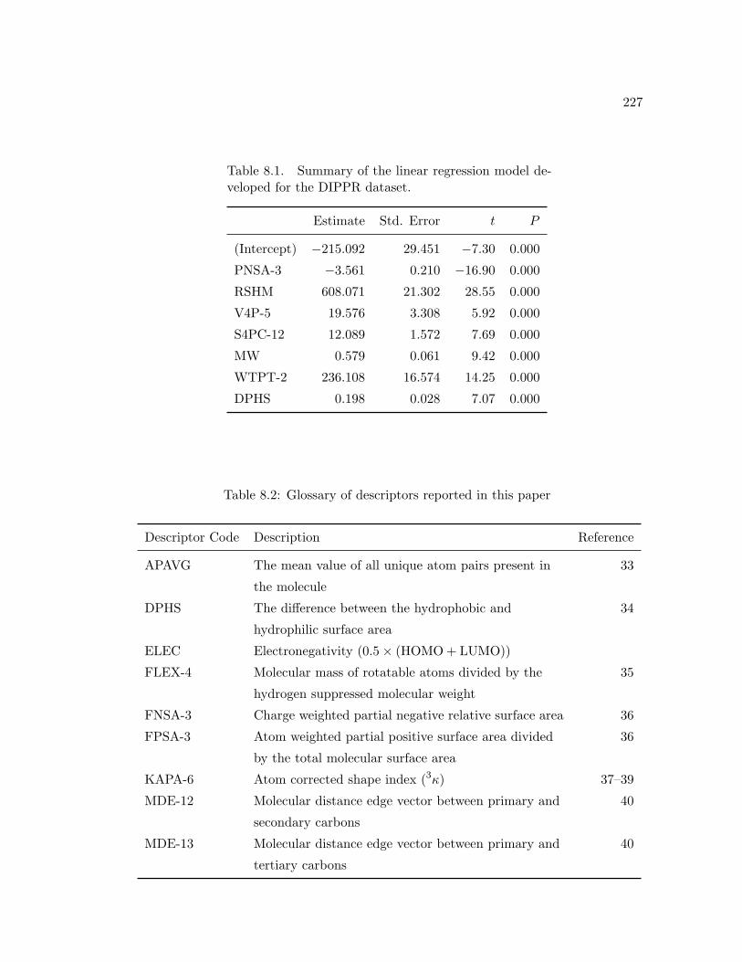
We first consider the linear and CNN models for the DIPPR dataset for modeling
boiling points. The statistics of the linear regression model for this dataset are summa-
rized in Table 8.1 and the meanings of the descriptors used in the model are summarized
in Table 8.2. The R2 value was 0.98, and the F -statistic was 1001 (for 7 and 139 degrees
of freedom) which is much greater than the critical value of 2.076 (α = 0.05). The model
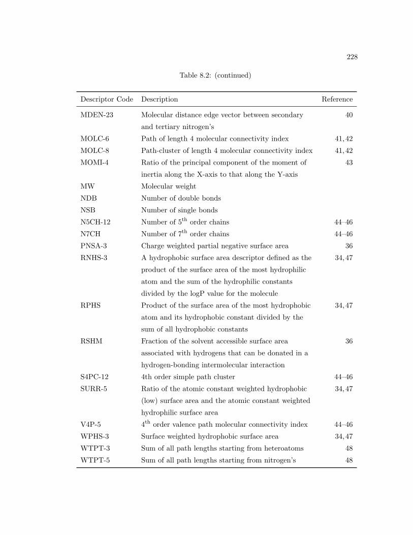
is thus statistically valid. The corresponding PLS analysis is summarized in Table 8.3.

221
The PLS statistics indicate that the increase in Q2 beyond the fourth component is neg-
ligible. Thus, we need only consider the most important descriptors in the first three
components. To see which descriptor is contributing the most in a given component, we
consider the X weights obtained from the PLS analysis which are displayed in Table 8.4.
In component 1 it is clear that MW and V4P-5 are the most heavily weighted descrip-
tors. Higher values of molecular weight correspond to larger molecules and thus elevated
boiling points. The V4P-5 descriptor characterizes branching in the molecular structure,
and higher values indicate a higher degree of branching. Thus, both of the most impor-
tant descriptors in the first component correlate molecular size to higher values of boiling
point. In the second component we see that the most weighted descriptors are RSHM
and PNSA-3. RSHM characterizes the fraction of the solvent accessible surface area
associated with hydrogens that can be donated in a hydrogen-bonding intermolecular
interaction. PNSA-3 is the charge weighted partial negative surface area. Clearly, both
these descriptors characterize the ability of molecules to form hydrogen bonds. In sum-
mary, the structure-property relationship captured by the linear model indicates that
London forces dominate the relationship. Although individual atomic contributions to
the trend are small, larger molecules will have more interactions leading to higher boiling
points. In addition, attractive forces, originating from hydrogen bond formation, also
play a role in the relationship and these are characterized in the second component of the
PLS model. We can use the above discussion and information from the PLS analysis to
rank the descriptors considered in the PLS analysis in decreasing order of contributions:
MW, V4P-5, RSHM, PNSA-3.
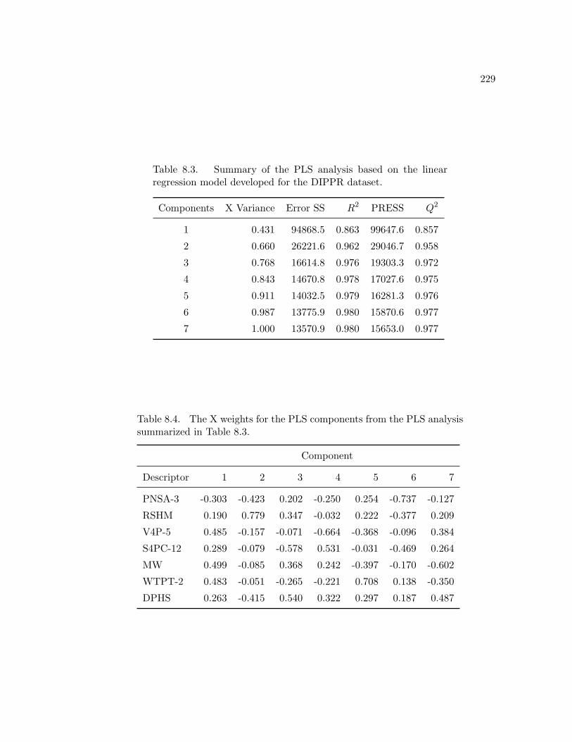
The next step was to develop a computational neural network model for this
dataset. The ADAPT methodology was used to search for descriptor subsets ranging in
size from 4 to 6. The final CNN model had a 5–3–1 architecture, and the statistics of the
model are reported in Table 8.5. The descriptors in this model were FNSA-3, MOLC-6,
WPHS-3 and RPHS, which are described in Table 8.2. The increase in RMSE values for
the descriptors in each neural network model are reported in Tables 8.6, 8.7 and 8.8. In
each table the third column represents the increase in RMSE, due to the scrambling of
the corresponding descriptor, over the base RMSE. It is evident that scrambling some
descriptors leads to larger increases, whereas others lead to negligible increases in the
RMSE. The information contained in these tables is more easily seen in the descriptor
importance plots shown in Figs. 8.1, 8.2 and 8.3. These figures plot the increase in
RMSE for each descriptor, in decreasing order.
222
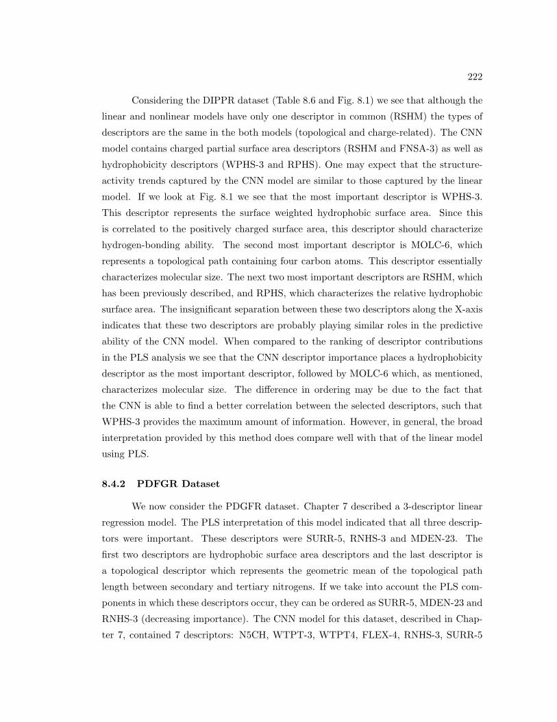
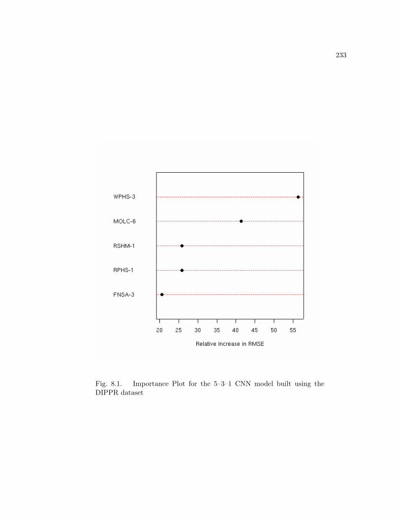
Considering the DIPPR dataset (Table 8.6 and Fig. 8.1) we see that although the
linear and nonlinear models have only one descriptor in common (RSHM) the types of
descriptors are the same in the both models (topological and charge-related). The CNN
model contains charged partial surface area descriptors (RSHM and FNSA-3) as well as
hydrophobicity descriptors (WPHS-3 and RPHS). One may expect that the structure-
activity trends captured by the CNN model are similar to those captured by the linear
model. If we look at Fig. 8.1 we see that the most important descriptor is WPHS-3.
This descriptor represents the surface weighted hydrophobic surface area. Since this
is correlated to the positively charged surface area, this descriptor should characterize
hydrogen-bonding ability. The second most important descriptor is MOLC-6, which
represents a topological path containing four carbon atoms. This descriptor essentially
characterizes molecular size. The next two most important descriptors are RSHM, which
has been previously described, and RPHS, which characterizes the relative hydrophobic
surface area. The insignificant separation between these two descriptors along the X-axis
indicates that these two descriptors are probably playing similar roles in the predictive
ability of the CNN model. When compared to the ranking of descriptor contributions
in the PLS analysis we see that the CNN descriptor importance places a hydrophobicity
descriptor as the most important descriptor, followed by MOLC-6 which, as mentioned,
characterizes molecular size. The difference in ordering may be due to the fact that
the CNN is able to find a better correlation between the selected descriptors, such that
WPHS-3 provides the maximum amount of information. However, in general, the broad
interpretation provided by this method does compare well with that of the linear model
using PLS.
8.4.2 PDFGR Dataset
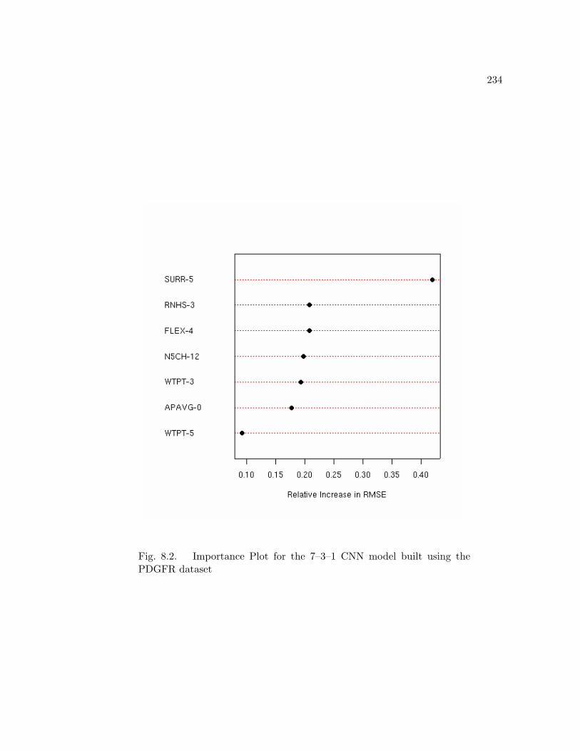
We now consider the PDGFR dataset. Chapter 7 described a 3-descriptor linear
regression model. The PLS interpretation of this model indicated that all three descrip-
tors were important. These descriptors were SURR-5, RNHS-3 and MDEN-23. The
first two descriptors are hydrophobic surface area descriptors and the last descriptor is
a topological descriptor which represents the geometric mean of the topological path
length between secondary and tertiary nitrogens. If we take into account the PLS com-
ponents in which these descriptors occur, they can be ordered as SURR-5, MDEN-23 and
RNHS-3 (decreasing importance). The CNN model for this dataset, described in Chap-
ter 7, contained 7 descriptors: N5CH, WTPT-3, WTPT4, FLEX-4, RNHS-3, SURR-5
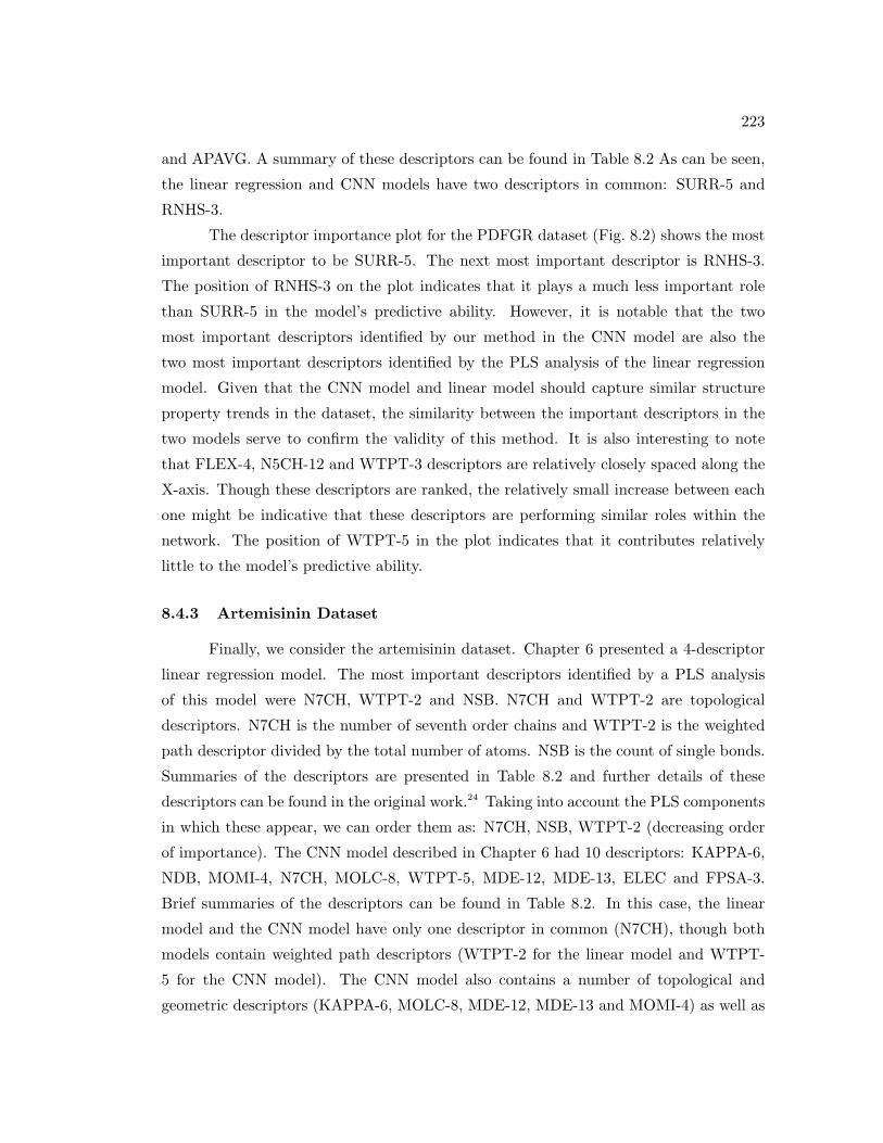
223
and APAVG. A summary of these descriptors can be found in Table 8.2 As can be seen,
the linear regression and CNN models have two descriptors in common: SURR-5 and
RNHS-3.
The descriptor importance plot for the PDFGR dataset (Fig. 8.2) shows the most
important descriptor to be SURR-5. The next most important descriptor is RNHS-3.
The position of RNHS-3 on the plot indicates that it plays a much less important role
than SURR-5 in the model’s predictive ability. However, it is notable that the two
most important descriptors identified by our method in the CNN model are also the
two most important descriptors identified by the PLS analysis of the linear regression
model. Given that the CNN model and linear model should capture similar structure
property trends in the dataset, the similarity between the important descriptors in the
two models serve to confirm the validity of this method. It is also interesting to note
that FLEX-4, N5CH-12 and WTPT-3 descriptors are relatively closely spaced along the
X-axis. Though these descriptors are ranked, the relatively small increase between each
one might be indicative that these descriptors are performing similar roles within the
network. The position of WTPT-5 in the plot indicates that it contributes relatively
little to the model’s predictive ability.
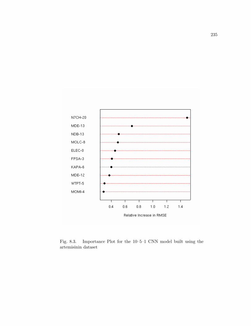
8.4.3 Artemisinin Dataset
Finally, we consider the artemisinin dataset. Chapter 6 presented a 4-descriptor
linear regression model. The most important descriptors identified by a PLS analysis
of this model were N7CH, WTPT-2 and NSB. N7CH and WTPT-2 are topological
descriptors. N7CH is the number of seventh order chains and WTPT-2 is the weighted
path descriptor divided by the total number of atoms. NSB is the count of single bonds.
Summaries of the descriptors are presented in Table 8.2 and further details of these
descriptors can be found in the original work.24 Taking into account the PLS components
in which these appear, we can order them as: N7CH, NSB, WTPT-2 (decreasing order
of importance). The CNN model described in Chapter 6 had 10 descriptors: KAPPA-6,
NDB, MOMI-4, N7CH, MOLC-8, WTPT-5, MDE-12, MDE-13, ELEC and FPSA-3.
Brief summaries of the descriptors can be found in Table 8.2. In this case, the linear
model and the CNN model have only one descriptor in common (N7CH), though both
models contain weighted path descriptors (WTPT-2 for the linear model and WTPT-
5 for the CNN model). The CNN model also contains a number of topological and
geometric descriptors (KAPPA-6, MOLC-8, MDE-12, MDE-13 and MOMI-4) as well as
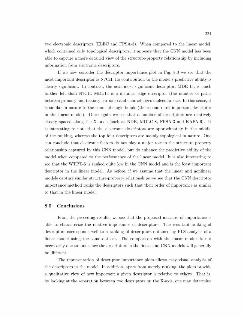
224
two electronic descriptors (ELEC and FPSA-3). When compared to the linear model,
which contained only topological descriptors, it appears that the CNN model has been
able to capture a more detailed view of the structure-property relationship by including
information from electronic descriptors.
If we now consider the descriptor importance plot in Fig. 8.3 we see that the
most important descriptor is N7CH. Its contribution to the model’s predictive ability is
clearly significant. In contrast, the next most significant descriptor, MDE-13, is much
further left than N7CH. MDE13 is a distance edge descriptor (the number of paths
between primary and tertiary carbons) and characterizes molecular size. In this sense, it
is similar in nature to the count of single bonds (the second most important descriptor
in the linear model). Once again we see that a number of descriptors are relatively
closely spaced along the X- axis (such as NDB, MOLC-8, FPSA-3 and KAPA-6). It
is interesting to note that the electronic descriptors are approximately in the middle
of the ranking, whereas the top four descriptors are mainly topological in nature. One
can conclude that electronic factors do not play a major role in the structure property
relationship captured by this CNN model, but do enhance the predictive ability of the
model when compared to the performance of the linear model. It is also interesting to
see that the WTPT-5 is ranked quite low in the CNN model and is the least important
descriptor in the linear model. As before, if we assume that the linear and nonlinear
models capture similar structure-property relationships we see that the CNN descriptor
importance method ranks the descriptors such that their order of importance is similar
to that in the linear model.
8.5 Conclusions
From the preceding results, we see that the proposed measure of importance is
able to characterize the relative importance of descriptors. The resultant ranking of
descriptors corresponds well to a ranking of descriptors obtained by PLS analysis of a
linear model using the same dataset. The comparison with the linear models is not
necessarily one-to- one since the descriptors in the linear and CNN models will generally
be different.
The representation of descriptor importance plots allows easy visual analysis of
the descriptors in the model. In addition, apart from merely ranking, the plots provide
a qualitative view of how important a given descriptor is relative to others. That is,
by looking at the separation between two descriptors on the X-axis, one may determine
225
that a certain descriptor plays a much more significant role than another in the model’s
predictive power. We conjecture that descriptors with little separation along the X-axis
play similar roles within the CNN architecture. However, confirmation of this requires
a more detailed interpretation of the CNN model, which we present in the next chapter.
It is clear that the proposed measure of descriptor importance does not allow
the user to elucidate exactly how the model represents the information captured by a
given descriptor. That is, the methodology does not indicate the sign (or direction)
of the effect of each input descriptor. Thus we cannot draw conclusions regarding the
nature of the correlation between input descriptors and network output. However, even
in the absence of a detailed understanding of the behavior of the input descriptors,
the method described here allows the user to determine the most important descriptor
(or descriptors) and investigate whether replacement by similar descriptors might lead
to an improvement in the model’s predictive ability. We investigated this possibility
by replacing the SURR-5 descriptor from the 10–5–1 CNN model for the artemisinin
dataset by other hydrophobic surface area descriptors. In some cases the RMSE of
the resultant model did increase, though not significantly. However in a few cases the
RMSE of the model decreased, compared to the original RMSE. This is not surprising,
as the importance plots show that theoretically related descriptors (such as WTPT-3
and WTPT-5 in Fig. 8.2) may have significantly different contributions. However, the
importance measure does allow us to change model descriptors in a guided manner. This
procedure is functionally similar to feature selection but the main difference is that it is
applied to a subset of descriptors that have already been deemed “good” by a feature
selection algorithm (genetic algorithm12 or simulated annealing25). Hence, the result of
the “tweaking” procedure described here, is akin to locally fine-tuning a given descriptor
subset, rather than selecting whole new subsets.
Finally, we note that the machine learning literature describes a number of ap-
proaches to interpretation of CNN models. In general, these methods are closely tied to
specific types of neural network models.8,9 A useful feature of this interpretation method-
ology is that it is quite general in nature. That is, the methodology is not dependent on
the specific characteristics of a neural network and depends only on the input data. This
implies that the methodology can be applied to obtain descriptor importance measures
for any type of neural network model such as single layer or multilayer perceptrons26
or radial basis networks.27 Furthermore many interpretation methods are focused on
extracting rules or analytical forms of the CNN’s internal model.28–30 In many cases,
this necessitates a complex analysis of the model utilizing another pattern recognition31

226
or optimization algorithm.28,32 In contrast, the method described here is simple to carry
out and provides easily understandable conclusions. In summary, the interpretation
methodology described here provides a broad view of descriptor importance for a neural
network model, thus alleviating the black box nature of the neural network methodology
to some extent.
227
Table 8.1. Summary of the linear regression model de-veloped for the DIPPR dataset.
Estimate Std. Error t P
(Intercept) −215.092 29.451 −7.30 0.000
PNSA-3 −3.561 0.210 −16.90 0.000
RSHM 608.071 21.302 28.55 0.000
V4P-5 19.576 3.308 5.92 0.000
S4PC-12 12.089 1.572 7.69 0.000
MW 0.579 0.061 9.42 0.000
WTPT-2 236.108 16.574 14.25 0.000
DPHS 0.198 0.028 7.07 0.000
Table 8.2: Glossary of descriptors reported in this paper
Descriptor Code Description Reference
APAVG The mean value of all unique atom pairs present in
the molecule
33
DPHS The difference between the hydrophobic and
hydrophilic surface area
34
ELEC Electronegativity (0.5× (HOMO + LUMO))
FLEX-4 Molecular mass of rotatable atoms divided by the
hydrogen suppressed molecular weight
35
FNSA-3 Charge weighted partial negative relative surface area 36
FPSA-3 Atom weighted partial positive surface area divided
by the total molecular surface area
36
KAPA-6 Atom corrected shape index (3κ) 37–39
MDE-12 Molecular distance edge vector between primary and
secondary carbons
40
MDE-13 Molecular distance edge vector between primary and
tertiary carbons
40
228
Table 8.2: (continued)
Descriptor Code Description Reference
MDEN-23 Molecular distance edge vector between secondary
and tertiary nitrogen’s
40
MOLC-6 Path of length 4 molecular connectivity index 41,42
MOLC-8 Path-cluster of length 4 molecular connectivity index 41,42
MOMI-4 Ratio of the principal component of the moment of
inertia along the X-axis to that along the Y-axis
43
MW Molecular weight
NDB Number of double bonds
NSB Number of single bonds
N5CH-12 Number of 5th order chains 44–46
N7CH Number of 7th order chains 44–46
PNSA-3 Charge weighted partial negative surface area 36
RNHS-3 A hydrophobic surface area descriptor defined as the
product of the surface area of the most hydrophilic
atom and the sum of the hydrophilic constants
divided by the logP value for the molecule
34,47
RPHS Product of the surface area of the most hydrophobic
atom and its hydrophobic constant divided by the
sum of all hydrophobic constants
34,47
RSHM Fraction of the solvent accessible surface area
associated with hydrogens that can be donated in a
hydrogen-bonding intermolecular interaction
36
S4PC-12 4th order simple path cluster 44–46
SURR-5 Ratio of the atomic constant weighted hydrophobic
(low) surface area and the atomic constant weighted
hydrophilic surface area
34,47
V4P-5 4th order valence path molecular connectivity index 44–46
WPHS-3 Surface weighted hydrophobic surface area 34,47
WTPT-3 Sum of all path lengths starting from heteroatoms 48
WTPT-5 Sum of all path lengths starting from nitrogen’s 48
229
Table 8.3. Summary of the PLS analysis based on the linearregression model developed for the DIPPR dataset.
Components X Variance Error SS R2 PRESS Q2
1 0.431 94868.5 0.863 99647.6 0.857
2 0.660 26221.6 0.962 29046.7 0.958
3 0.768 16614.8 0.976 19303.3 0.972
4 0.843 14670.8 0.978 17027.6 0.975
5 0.911 14032.5 0.979 16281.3 0.976
6 0.987 13775.9 0.980 15870.6 0.977
7 1.000 13570.9 0.980 15653.0 0.977
Table 8.4. The X weights for the PLS components from the PLS analysissummarized in Table 8.3.
Component
Descriptor 1 2 3 4 5 6 7
PNSA-3 -0.303 -0.423 0.202 -0.250 0.254 -0.737 -0.127
RSHM 0.190 0.779 0.347 -0.032 0.222 -0.377 0.209
V4P-5 0.485 -0.157 -0.071 -0.664 -0.368 -0.096 0.384
S4PC-12 0.289 -0.079 -0.578 0.531 -0.031 -0.469 0.264
MW 0.499 -0.085 0.368 0.242 -0.397 -0.170 -0.602
WTPT-2 0.483 -0.051 -0.265 -0.221 0.708 0.138 -0.350
DPHS 0.263 -0.415 0.540 0.322 0.297 0.187 0.487
230
Table 8.5. Summarystatistics for the best CNNmodel for the DIPPRdataset. The modelarchitecture was 5–3–1.
R2 RMSE
TSET 0.98 9.92
CVSET 0.99 7.89
PSET 0.98 8.61
Table 8.6. Increase in RMSE due to scrambling ofindividual descriptors. The CNN architecture was5–3–1 and as built using the DIPPR dataset. Thebase RMSE was 9.92
Scrambled Descriptor RMSE Difference
1 FNSA-3 30.50 20.58
2 RSHM 35.76 25.84
3 MOLC-6 51.32 41.39
4 WPHS-3 66.27 56.35
5 RPHS 35.75 25.83
231
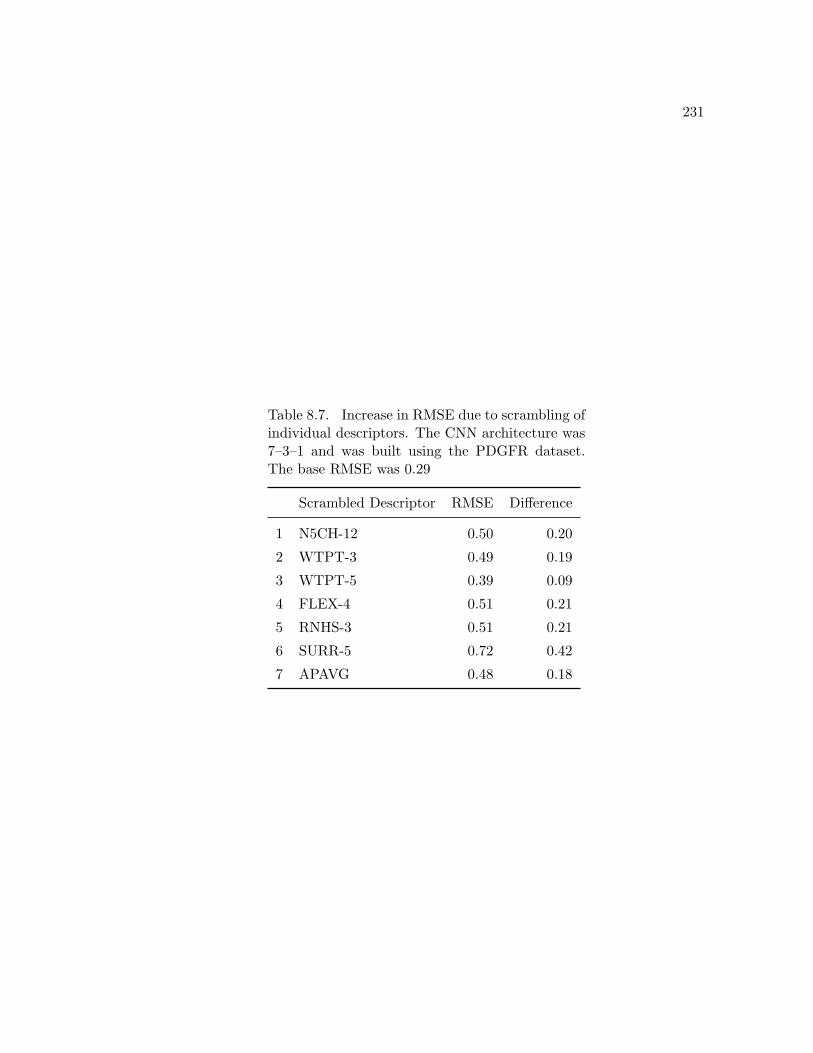
Table 8.7. Increase in RMSE due to scrambling ofindividual descriptors. The CNN architecture was7–3–1 and was built using the PDGFR dataset.The base RMSE was 0.29
Scrambled Descriptor RMSE Difference
1 N5CH-12 0.50 0.20
2 WTPT-3 0.49 0.19
3 WTPT-5 0.39 0.09
4 FLEX-4 0.51 0.21
5 RNHS-3 0.51 0.21
6 SURR-5 0.72 0.42
7 APAVG 0.48 0.18
232
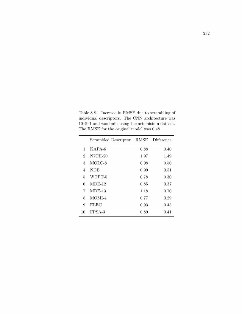
Table 8.8. Increase in RMSE due to scrambling ofindividual descriptors. The CNN architecture was10–5–1 and was built using the artemisinin dataset.The RMSE for the original model was 0.48
Scrambled Descriptor RMSE Difference
1 KAPA-6 0.88 0.40
2 N7CH-20 1.97 1.49
3 MOLC-8 0.98 0.50
4 NDB 0.99 0.51
5 WTPT-5 0.78 0.30
6 MDE-12 0.85 0.37
7 MDE-13 1.18 0.70
8 MOMI-4 0.77 0.29
9 ELEC 0.93 0.45
10 FPSA-3 0.89 0.41
233
Fig. 8.1. Importance Plot for the 5–3–1 CNN model built using theDIPPR dataset
234
Fig. 8.2. Importance Plot for the 7–3–1 CNN model built using thePDGFR dataset
235
Fig. 8.3. Importance Plot for the 10–5–1 CNN model built using theartemisinin dataset
236
References
[1] Kohonen, T. Self Organizing Maps; Springer: Berlin, 1994.
[2] Castro, J.; Mantas, C.; Benitez, J. Interpretation of Artificial Neural Networks by
Means of Fuzzy Rules. IEEE Trans. Neural Networks 2002, 13, 101–116.
[3] Jones, W.; Vachha, R.; Kulshrestha, A. DENDRITE: A System for Visual Inter-
pretation of Neural Network Data. In Southeastcon, Proceedings of, Vol. 2; IEEE:
New York, NY, 1992.
[4] Limin, F. Rule Generation from Neural Networks. IEEE Trans. Systems, Man and
Cybernetics 1994, 24, 1114–1124.
[5] Ney, H. On the Probabilistic Interpretation of Neural Network Classifiers and Dis-
criminative Training Criteria. IEEE Trans. Pat. Anal. Mach. Intell. 1995, 17, 107–
119.
[6] Taha, I.; Ghosh, J. Symbolic Interpretation of Artificial Neural Networks. IEEE
Trans. Knowl. Data Eng. 1999, 11, 448–463.
[7] Takahashi, T. An Information Theoretical Interpretation of Neuronal Activities. In
Neural Networks, International Joint Conference on, Vol. 2; IEEE: New York, NY,
1991.
[8] Bologna, G. Rule Extraction from Linear Combinations of DIMLP Neural Networks.
In Proceedings of the Sixth Brazilian Symposium on Neural Networks; IEEE: New
York, NY, 2000.
[9] Hervas, C.; Silva, M.; Serrano, J. M.; Orejuela, E. Heuristic Extraction of Rules in
Pruned Artificial Neural Network Models Used for Quantifying Highly Overlapping
Chromatographic Peaks. J. Chem. Inf. Comput. Sci. 2004, 44, 1576–1584.
[10] Jurs, P.; Chou, J.; Yuan, M. Studies of Chemical Structure Biological Activity
Relations Using Pattern Recognition. In Computer assisted drug design; Olsen, E.;
Christoffersen, R., Eds.; American Chemical Society: Washington D.C., 1979.
[11] Stuper, A.; Brugger, W.; Jurs, P. Computer Assisted Studies of Chemical Structure
and Biological Function; Wiley: New York, 1979.
237
[12] Goldberg, D. Genetic Algorithms in Search Optimization & Machine Learning; Ad-
dison Wesley: Reading, MA, 2000.
[13] Wessel, M. Computer Assisted Development of Quantitative Structure-Property Re-
lationships And Design of Feature Selection Routines, PhD thesis, Pennsylvania
State University, 1997.
[14] So, S.-S.; Karplus, M. Evolutionary Optimization in Quantitative Structure-
Activity Relationship: An Application of Genetic Neural Networks. J. Med. Chem.
1996, 39, 1521–1530.
[15] Breiman, L. Random forests. Machine Learning 2001, 45, 5–32.
[16] Breiman, L.; Friedman, J.; Olshen, R.; Stone, C. Classification and Regression
Trees; CRC Press: Boca Raton, FL, 1984.
[17] Stanton, D. On the Physical Interpretation of QSAR Models. J. Chem. Inf. Com-
put. Sci. 2003, 43, 1423–1433.
[18] Goll, E.; Jurs, P. Prediction of the Normal Boiling Points of Organic Com-
pounds from Molecular Structures with a Computational Neural Network Model.
J. Chem. Inf. Comput. Sci. 1999, 39, 974–983.
[19] Lu, X.; Ball, J.; Dixon, S.; Jurs, P. Quantitative Structure-Activity Relation-
ships for Toxicity of Phenols Using Regression Analysis and Computational Neural
Networks. Environ. Toxicol. Chem. 1994, 13, 841–851.
[20] Wessel, M.; Jurs, P. Prediction of Reduced Ion Mobility Constants from Structural
Information Using Multiple Linear Regression Analysis and Computational Neural
Networks. Anal. Chem. 1994, 66, 2480–2487.
[21] Cramer, R.; Patterson, D.; Bunce, J. Comparative Molecular Field Analy-
sis (CoMFA). I. Effect of Shape on Binding of Steroids to Carrier Protiens.
J. Am. Chem. Soc. 1988, 110, 5959–5967.
[22] Avery, M. A.; Alvim-Gaston, M.; Rodrigues, C. R.; Barreiro, E. J.; Cohen, F. E.;
Sabnis, Y. A.; Woolfrey, J. R. Structure Activity Relationships of the Antimalarial
Agent Artemisinin. the Development of Predictive in Vitro Potency Models Using
CoMFA and HQSAR Methodologies. J. Med. Chem. 2002, 45, 292–303.
238
[23] Pandey, A.; Volkots, D. L.; Seroogy, J. M.; Rose, J. W.; Yu, J.-C.; Lambing, J. L.;
Hutchaleelaha, A.; Hollenbach, S. J.; Abe, K.; Giese, N. A.; Scarborough, R. M.
Identification of Orally Active, Potent, and Selective 4-Piperazinylquinazolines as
Antagonists of the Platelet-Derived Growth Factor Receptor Tyrosine Kinase Fam-
ily. J. Med. Chem. 2002, 45, 3772–3793.
[24] Guha, R.; Jurs, P. C. The Development of QSAR Models to Predict and Interpret
the Biological Activity of Artemisinin Analogues. J. Chem. Inf. Comput. Sci. 2004,
44, 1440–1449.
[25] Sutter, J.; Dixon, S.; Jurs, P. Automated Descriptor Selection for Quanti-
tative Structure-Activity Relationships Using Generalized Simulated Annealing.
J. Chem. Inf. Comput. Sci. 1995, 35, 77–84.
[26] Haykin, S. Neural Networks; Pearson Education: Singapore, 2001.
[27] Patankar, S.; Jurs, P. Prediction of Glycine/NMDA Receptor Antagonist Inhibition
from Molecular Structure. J. Chem. Inf. Comput. Sci. 2002, 42, 1053–1068.
[28] Fu, X.; Wang, L. Rule Extraction by Genetic Algorithms Based on a Simplified RBF
Neural Network. In Evolutionary Computation, Proceedings of the 2001 Congress
on, Vol. 2; IEEE: New York, NY, 2001.
[29] Gupta, A.; Park, S.; Lam, S. Generalized Analytic Rule Extraction for Feedforward
Neural Networks. IEEE Trans. Knowl. Data Eng. 1999, 11, 985–991.
[30] Ishibuchi, H.; Nii, M.; Tanaka, K. Fuzzy-Arithmetic-Based Approach for Extracting
Positive and Negative Linguistic Rules from Trained Neural Networks. In Fuzzy
Systems, Proceedings of the IEEE International Conference on, Vol. 3; IEEE: New
York, NY, 1999.
[31] Chen, P.; Mills, J. Modeling of Neural Networks in Feedback Systems Using De-
scribing Functions. In Neural Networks, International Conference on, Vol. 2; IEEE:
New York, NY, 1997.
[32] Yao, S.; Wei, C.; He, Z. Evolving Fuzzy Neural Networks for Extracting Rules. In
Fuzzy Systems, Proceedings of the Fifth IEEE International Conference on, Vol. 1;
IEEE: New York, NY, 1996.
239
[33] Carhart, R.; Smith, D.; Venkataraghavan, R. Atom Pairs as Molecular Features in
Structure-Activity Studies: Definition and Application. J. Chem. Inf. Comput. Sci.
1985, 25, 64–73.
[34] Stanton, D.; Mattioni, B. E.; Knittel, J.; Jurs, P. Development and Use of
Hydrophobic Surface Area (HSA) Descriptors for Computer Assisted Quantita-
tive Structure-Activity and Structure-Property Relationships. J. Chem. Inf. Com-
put. Sci. 2004, 44, 1010–1023.
[35] Mosier, P. D.; Counterman, A. E.; Jurs, P. C.; Clemmer, D. E. Prediction of Pep-
tide Ion Collision Cross Sections from Topological Molecular Structure and Amino
Acid Parameters. Anal. Chem. 2002, 74, 1360–1370.
[36] Stanton, D.; Jurs, P. Development and Use of Charged Partial Surface Area Struc-
tural Descriptors in Computer Assissted Quantitative Structure Property Relation-
ship Studies. Anal. Chem. 1990, 62, 2323–2329.
[37] Kier, L. A Shape Index from Molecular Graphs. Quant. Struct.-Act. Relat. Phar-
macol.,Chem. Biol. 1985, 4, 109–116.
[38] Kier, L. Shape Indexes for Orders One and Three from Molecular Graphs.
Quant. Struct.-Act. Relat. Pharmacol.,Chem. Biol. 1986, 5, 1–7.
[39] Kier, L. Distinguishing Atom Differences in a Molecular Graph Index.
Quant. Struct.-Act. Relat. Pharmacol.,Chem. Biol. 1986, 5, 7–12.
[40] Liu, S.; Cao, C.; Li, Z. Approach to Estimation and Prediction for Normal Boiling
Point (NBP) of Alkanes Based on a Novel Molecular Distance Edge (MDE) Vector,
λ. J. Chem. Inf. Comput. Sci. 1998, 38, 387–394.
[41] Balaban, A. Higly Discriminating Distance Based Topological Index.
Chem. Phys. Lett. 1982, 89, 399–404.
[42] Kier, L.; Hall, L. Molecular Connectivity in Chemistry & Drug Research; Academic
Press: New York, 1976.
[43] Goldstein, H. Classical Mechanics; Addison Wesley: Reading, MA, 1950.
[44] Kier, L.; Hall, L.; Murray, W. Molecular Connectivity I: Relationship to Local
Anesthesia. J. Pharm. Sci. 1975, 64,.
240
[45] Kier, L.; Hall, L. Molecular Connectivity in Structure Activity Analysis; John Wiley
& Sons: Hertfordshire, England, 1986.
[46] Kier, L.; Hall, L. Molecular Connectivity VII: Specific Treatment to Heteroatoms.
J. Pharm. Sci. 1976, 65, 1806–1809.
[47] Mattioni, B. E. The Development of Quantitative Structure-Activity Relationship
Models for Physical Property and Biological Activity Prediction of Organic Com-
pounds, PhD thesis, Pennsylvania State University, 2003.
[48] Randic, M. On Molecular Idenitification Numbers. J. Chem. Inf. Comput. Sci.
1984, 24, 164–175.