neural network and multiple regression models for

The Egyptian Int. J. of Eng. Sci. and Technology

Vol. 15, No. 1 (Jan. 2012)

Emad E. Elbeltagi 1, Hossam H. Mohamed

2, Dhaheer A. Thabet

2**

1 Structural Eng. Dept., Mansoura Univ., Egypt.

2 Construction and Utilities Eng. Dept., Zagazig Univ., Egypt.

ABSTRACT

Production rate estimation is one of the most frequently discussed topics in construction industry. Production

rates of excavation operation in building construction are affected by several factors. Among these factors are:

hauling distance, loading area layout, dumping area layout, pile foundation, excavator bucket capacity, size and

number of hauling units. Consequently, estimation accuracy here is challenged when the effects of these

multiple factors are simultaneously considered. In this paper, a comprehensive review of literature and interview

with project managers were performed to identify the most significant factors affecting the production rates

excavation operations. Sixteen factors were identified as the most significant factors affect the production rates

of such operations. These factors were classified into three categories, namely: 1) Job - Site Conditions, 2)

Equipment Characteristics, 3) Management Conditions. The objective in this paper is the development of a

suitable tool that can be effectively used to predict the production rates of the excavation operation in building

construction projects. For this purpose, field observations were conducted to collect realistic production rates

over a period of twelve months (12/7/2009 to 17/7/2010) in the city of Alexandria (Egypt). Eighty-five actual

case studies taken from seventeen building projects were used as raw data to develop the proposed neural

network (NNM) and multiple regression (MRM) models. These data were randomly divided into two groups:

(1) training data (75 actual production rates), (2) validating data (10 actual production rates). In conclusion,

comparison between the predictive capabilities of both the best NNM and the best MRM indicates that the NNM

outperforms the MRM.

KEY WORDS: Production rates; Excavation operation; Neural network; Regression.

RESEAU NEURONAL ET DE MODELES DE REGRESSION MULTIPLE POUR L'ESTIMATION DES TAUX DE PRODUCTION DANS LES OPÉRATIONS DE EXCAVATION

RÉSUMÉ

Estimation du taux de production est l'un des sujets les plus fréquemment discutés dans l'industrie de la construction.

Les taux de production de l'opération de fouilles dans le bâtiment sont affectés par plusieurs facteurs. Parmi ces

facteurs sont: le transport à distance, le chargement structure de l'espace, le dumping mise en espace, fondation sur

pieux, la capacité de godet de l'excavatrice, la taille et le nombre d'unités de débardage. Par conséquent, sa précision

d'estimation pourrait être contestée lorsque les effets de ces multiples facteurs sont considérés simultanément. Dans ce

document de recherche à un examen complet de la littérature et des entrevues avec des gestionnaires de projet ont été

réalisées pour identifier les facteurs les plus importants qui affectent les taux de production de l'opération de fouilles.

Seize facteurs ont été identifiés comme les facteurs les plus importants qui affectent les taux de production de

l'opération d'excavation. Ces facteurs ont été classés en trois catégories, à savoir: 1) Job - Conditions du site, 2)

caractéristiques des équipements, 3) Condition de gestion. L'objectif de ce document de recherche est le

développement d'un outil adapté qui peut être efficacement utilisé pour prédire le taux de production de l'opération

d'excavation dans la construction de projets de construction. A cet effet, les observations de terrain ont été menées

pour collecter des taux de production réalistes sur une période de douze mois (07/12/2009 au 17/7/2010), à Alexandrie

- Egypte. Quatre-vingt-cinq études de cas réels tirés de dix-sept projets bâtiment construit à Alexandrie - Egypte ont

été utilisées comme données brutes pour développer le modèle de réseau neuronal proposé (NNM) et le modèle de

régression multiple (MRM). Ces données ont été répartis aléatoirement en deux groupes: (1) les données

d'entraînement (75 taux de production réels), (2) la validation des données (10 taux de production réels). En

conclusion, la comparaison entre les capacités prédictives des deux meilleurs NNM et la meilleure MRM a indiqué

que la NNM surperformé le MRM.

MOTS CLÉS: simulation, opération d'excavation, les rate de la production, le cost unitaire.

* Received: 12/7/2011, accepted: 11/9/2011 (Technical Paper)

** Contact author ([email protected], +2 012 812 90 947)

NEURAL NETWORK AND MULTIPLE REGRESSION MODELS FOR

ESTIMATION OF PRODUCTION RATES IN EXCAVATION OPERATIONS *

EIJEST

1

Neural Network and Multiple Regression Models for Estimation of Production Rates in Excavation Operations

Elbeltagi, Mohamed, Thabet

1. INTRODUCTION

Excavation operation is often one of the most

important operations in any construction project

in terms of its serious effect on both cost and

time of these projects. Production rates

estimation of excavation equipment generally

based on the company's historical data and

experts' opinion. In addition to these sources,

production rates in handbooks and information

from equipment suppliers are often used as

references for estimation. The inaccuracy of

production rates estimation is not only resulted

from ineffective verification, but is also caused

by the inconsistent consideration of the most

important factors affecting the production rates

of the excavation operation. Moreover, the

accuracy of the production rates estimation in the

planning phase could be challenged when the

effect of multiple factors is considered

simultaneously.

The duration of a construction project is usually

determined by the clients at the design stage and

is then documented in the bid documents.

Contractors are usually under an obligation to

evaluate the feasibility of the project duration

before a contract has been awarded. However,

time pressures typically do not allow contractors

to perform this analysis. Further complicating

the matter, clients frequently use inaccurate

production rates to estimate construction time.

Therefore, many projects are developed using

unrealistic contract time duration.

Using inaccurate production rates to estimate

construction time and cost has been recognized as a

major source of bias in cost and time estimation.

The only way to prevent inaccurate contract time

estimation is to use realistic production rates. This

research aims to develop NNM and MRM by using

the realistic production rates to assist the planners

and estimators to reduce the effort required for

planning excavation operation as well as to

improve the accuracy of production rates

estimation.

2. FACTORS AFFECTING

PRODUCTION RATES OF

EXCAVATION OPERATIONS

In this paper a comprehensive review of literature

and interview with project managers were

performed to identify the most significant factors

affecting the production rates of the excavation

operation.

Chao and Skibniewski (1994) performed a case

study in which a neural network was used to

predict the productivity of an excavator. Flood and

Christophilos7 (1996) modeled earthmoving

operations utilizing neural networks. Shi18

(1999)

developed an artificial neural network for

predicting earthmoving operations in a mining

reclamation project. Smith19

(1999) used linear

regression model to estimate the productivity of the

earthmoving operations in highway projects.

Edwards and Holt6 (2000) developed regression

model to calculate the excavator productivity and

output costs. Peurifoy et al.16

(2010) considered the

shovel machine as a dependent unit in the

excavation operation. They identified nine factors

affected the production rate of the shovel. Jonasson

et al.10

(2002) studied the productivity of earthwork

for different types of advanced positioning systems. Tam et al.

20 (2002) developed a quantitative model

for predicting the production rate of excavator

using artificial neural networks (ANN) to establish

a higher precision model. Bhurisith and Touran4

(2002) conducted a case study with regard to

obsolescence and equipment production rate and

the ideal production rates of wheel type loaders,

track-type loaders, scrapers, and crawler dozers. Hegazy and Kassab

8 (2003) presented a simple and

powerful approach for resource management and

optimization in construction projects using a

combination of flow chart-based simulation and

genetic algorithms (GAs). Two examples were

presented in this study to show the power and

diversity of the proposed GA-optimized simulation

planning approach: concrete-columns placing and

earthmoving operation at Hong Kong International

Airport. Marzouk and Moselhi11

(2003) presented a

simulation engine, developed to model

earthmoving operations. Marzouk and Moselhi12

(2004) presented a framework for optimizing

earthmoving operations using computer simulation

and genetic algorithms. Moselhi and Alshibani15

(2009) developed optimization model for

earthmoving operation in heavy civil engineering

projects.

Based on the above comprehensive review of

literature and interview with project managers

sixteen factors (Table 1) were identified as the most

significant factors affecting the production rates of

excavation operation. According to Table (1), such

factors were classified into three categories. Such

categories mainly include: Job- site Condition,

Equipment Characteristics and Management

Conditions.

2


Vol. 15, No. 1 (Jan. 2012)

Table 1: Factors affecting production rates of excavation operations

Category Description Factors included in Category Symbol

(1) Job- Site Conditions

(1) Loading area layout X1

(2) Dumping area layout X2

(3) Type of soil X3

(4) Excavation depth X4

(5) Haul distance X5

(6) Pile foundation X6

Weather conditions:

(7) Temperature

(8) Relative humidity

(9) Rainfall

X7

X8

X9

(2) Equipment Characteristics

(1) Excavator bucket capacity

(2) Maximum digging depth of excavator

X10

X11

(3) Swing angle X12

(4) Size of hauling units X13

(5) Number of hauling units X14

(3) Management Conditions (1) Efficiency of supervision X15

(2) Operator skill X16

3. DATA COLLECTION

In this research, the production rates of the

excavation operation for building foundation will be

defined as the total amount of material loaded by the

excavator to the trucks, the trucks once loaded, haul

to the dump area, dump the load and return to the

queue in a unit time such as a minute or an hour. A

field observation is conducted by the researcher over

a period of twelve months (12/7/2009 to 17/7/2010)

in the city of Alexandria (Egypt). A data collection

form was designed for collecting the required data. A

total number of eighty-five actual case studies were

collected from seventeen construction projects.

These data were divided into two groups randomly:

(1) training data (75 actual production rates), (2)

validating data (10 actual production rates). The

collected data of these cases mainly include the

production rates of excavation operation as well as

the different factors affecting such production. For

further information, the reader is referred to Thabet21

(2011).

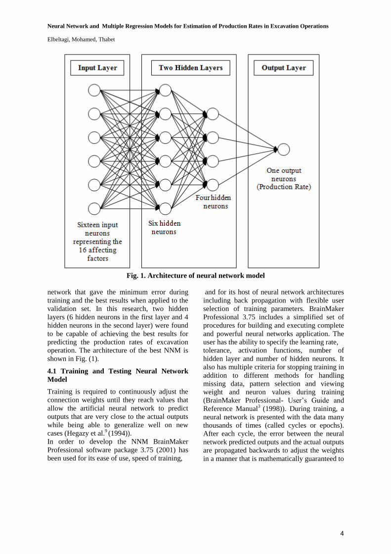
4. ARCHITECTURE OF NEURAL

NETWORK MODEL

The sixteen factors that listed in Table (1) and

the production rates are used as input and output

neurons of the back-propagation neural

network, respectively. To determine the number

of hidden layers, Bailey and Thompson2 (1990)

suggested, as a rule of thumb, start with one

hidden layer and add more as long as the

performance of the network is improved. The

size of the hidden layer (number of hidden

neurons) can be specified by using a number of

heuristics including: 1) Bailey and Thompson2

(1990) suggested the number of neurons to be

around 75% of the size of the input layer, 2)

BrainMaker Professional user’s guide3 (1998)

suggested that the number of neurons in hidden

layer to be as per the following formula:

… (1)

All the above recommendations are considered

as a first step to develop the present model.

Moreover, Moselhi et al.14

(1991) advised that

the proper number is determined by the

experimentations. Therefore, for verifying this

work, the traditional trial and error process was

performed in order to reach the best possible

3



Fig. 1. Architecture of neural network model

network that gave the minimum error during

training and the best results when applied to the

validation set. In this research, two hidden

layers (6 hidden neurons in the first layer and 4

hidden neurons in the second layer) were found

to be capable of achieving the best results for

predicting the production rates of excavation

operation. The architecture of the best NNM is

shown in Fig. (1).

4.1 Training and Testing Neural Network

Model

Training is required to continuously adjust the

connection weights until they reach values that

allow the artificial neural network to predict

outputs that are very close to the actual outputs

while being able to generalize well on new

cases (Hegazy et al.9 (1994)).

In order to develop the NNM BrainMaker

Professional software package 3.75 (2001) has

been used for its ease of use, speed of training,

and for its host of neural network architectures

including back propagation with flexible user

selection of training parameters. BrainMaker

Professional 3.75 includes a simplified set of

procedures for building and executing complete

and powerful neural networks application. The

user has the ability to specify the learning rate,

tolerance, activation functions, number of

hidden layer and number of hidden neurons. It

also has multiple criteria for stopping training in

addition to different methods for handling

missing data, pattern selection and viewing

weight and neuron values during training

(BrainMaker Professional- User’s Guide and

Reference Manual3

(1998)). During training, a

neural network is presented with the data many

thousands of times (called cycles or epochs).

After each cycle, the error between the neural

network predicted outputs and the actual outputs

are propagated backwards to adjust the weights

in a manner that is mathematically guaranteed to

4


Vol. 15, No. 1 (Jan. 2012)

Fig. 2. Statistical graph of training results

Table 2: NNM architecture, parameters and training results

NNM Architecture

Learning

Rate Tolerance

Transfer

Function

RMS

Error Input

layer

First

Hidden

Layer

Second

Hidden Layer

Output

Layer

16 6 4 1 0.1 0.1 Sigmoid 6.08 %

converge (Rumelhart et al.17

(1986)). Several

training experiments were conducted to arrive at

the best training model.

In these experiments, parameters of the

networks structure such as the number of hidden

layers, the number of hidden neurons, learning

rate, tolerance, and transfer function such as

sigmoid function, linear function, and other

functions available on the software were

changed and the best results were documented.

After training the network, the user can evaluate

the training and testing processes by using the

training and testing statistical files. The best

model was selected based on reaching

acceptable minimum values of the root mean

square error (RMS Error). The collected data

were divided into two sections, training data (90

% of the training data set) and testing data (10

% of the training data set). The training RMS

Error for the network is the average of the root

square of the difference between the actual and

predicted outputs for the training data set. The

testing RMS Error for the network is the

average of the root square of the difference

between the actual and predicted outputs for the

testing data.

The mean squared error equation is:

2 ………... (2)

Where RMS Error = root mean square error; N

= number of cases; A = actual production rate; P

= predicted production rate.

During training, the RMS Error between the

actual and predicted values for the production

rates was plotted as shown in Fig. (2). It was

clear that the error decreased as the number of

runs increase and then become stable. The

network used as the best model for this research

that trained and tested successfully has a

minimum RMS Error of approximately 6.08 %.

The network stabilized at this error rate and

training was stopped at 4924 runs. The architec-

5



Table 3: NNM validation results

No. of Cases Actual Production Rates Predicted Production

Rates Error

1 375 363.84 11.16

2 445 409.83 35.17

3 338 363.17 - 25.17

4 454 445.37 8.63

5 1067 1020.7 46.3

6 492 487.14 4.86

7 1040 1044.3 - 4.3

8 430 428.49 1.51

9 368 405.38 - 37.38

10 694 725.97 - 31.97

RMS Error = 8.17 %

MAPE = 4.11 %

R2 = 0.991

ture, parameters and training results of the best

NNM are tabulated in Table (2).

4.2 Neural Network Model Validation

Once the network was trained and a satisfactory

error level was achieved, the validation data that

had not been presented to the network during

training were used to check how well the trained

model predicts the production rates that it has

never seen before. Three evaluation parameters

were used as a basis for evaluating the

performance of the trained neural network model:

(1) Root mean square error (RMS Error); (2)

Mean absolute percentage error (MAPE); (3)

adjusted square multiple R (R2). Mathematically,

these parameters are defined as follows:

2 ……………… (3)

…………..(4)

Where N= number of cases; A= actual value; P=

predicted value.

The results of the validation process were

summarized in Table (3). As shown in Table (3),

the RMS Error, MAPE and R2 were found to be

8.17 %, 4.11% and 0.991 respectively. These

results reveal that the developed model has

excellent predictive capabilities.

5. REGRESSION ANALYSIS

Many problems in engineering and science

involve exploring the relationships between two or

more variables. Regression analysis is a statistical

technique that is very useful for these types of

problems (Montgomery and Runger13

(2010)).

The multiple regression model (MRM) will be

used to determine the statistical relationship

between a response or dependent variable (e.g.

actual production rate) and the explanatory

variables or independent variables (e.g., excavator

bucket capacity, haul distance, or truck capacity).

The responses to the regression model are what

the planning engineer ultimately wants to

estimate.

6


Vol. 15, No. 1 (Jan. 2012)

Table 4: MRM 1- using stepwise technique

Adjusted square multiple R = 0.962

F ratio = 316.413 , P- value = 0.00

Variables Coefficients t-ratio Partial F

Constant - 667.668 -7.970 0.000

Excavator bucket

capacity 251.693 2.082 0.041

Type of soil 12.923 1.979 0.052

Haul distance -61.161 -8.534 0.000

Haul unit number 94.435 9.515 0.000

Haul unit size 68.885 9.263 0.000

Loading area layout 39.351 3.368 0.001

Table 5: MRM 2 – using backward technique


F ratio = 283.043 , P- value = 0.00


Constant -567.305 -4.652 0.000

Dumping area

layout 48.811 4.002 0.000

Type of soil 18.218 2.596 0.012

Haul distance -65.581 -9.803 0.000

Haul unit size 68.784 9.349 0.000

Obstacles -78.518 -2.301 0.024

Haul unit number 104.443 16.784 0.000

Loading area layout 16.516 2.275 0.026

The MRM is given by the equation:

)6..(..........22110 ipp xxxY

i = 1, 2, …n

and assuming the following:

• is the response that corresponds to the levels

of the explanatory variables x1, x2,…, xp at the

i th observation.

• p ,...,, 10 are the coefficients in the linear

relationship. For a single factor (p = 1), 0 is

the intercept, and is the slope of the straight

line defined.

• n ,...,, 21 are the errors that create scatter

around the linear relationship at each of the i = 1

to n observations.

To make estimates of the coefficients in the

regression model, the method of least squares is

used for both its mathematical convenience and

its ability to provide explicit expressions for

these estimates (Smith19

(1999)).

7



Table 6: MRM 3 – using forward technique


F ratio = 288.107, P- value = 0.00


Constant -527.090 -4.284 0.000

Excavator bucket

capacity 231.864 1.927 0.058

Type of soil 17.509 2.462 0.016

Haul distance -60.248 -8.463 0.000

Obstacles -69.10 -1.547 0.127

Haul unit size 87.296 8.042 0.000

Haul unit number 62.528 7.416 0.000

Dump area layout 46.895 3.736 0.000

5.1 Regression Model Development

Various regression models for excavation

operations were developed using statistical

analysis techniques (stepwise, backward, and

forward techniques). The SPSS 18 package, which

was used to analyze the data and develop the

models, provides the user with the ability to select

one of the three different techniques.

The collected data set was divided randomly into

two main groups: model developing (75

observations), and validation (10 observations)

data sets. These data were organized and saved in

Microsoft Excel spreadsheet. The SPSS 18

package is compatible with Microsoft Excel.

Therefore, the data exported from Excel to SPSS

using the file import option in SPSS.

For a model, that includes sixteen variables with

the use of seventy-five case case studies:

Fcritical = F , p-1, n-p = F0.05, 16, 58 = 1.84..….. (7)

where n= number of observations, which equal to

eighty-five; p= independent variables in the

complete model, which equal to sixteen variables

plus the constant (total 17). P-1= number of

degree of freedom for the regression, n-p = degree

of freedom for the error.

Several modelling experiments took place; the

three most suitable models are shown in Tables

(4), (5) and (6).

Based on the statistical tests, it can be concluded

that the regression model produced by using the

backward technique is more useful in predicting the dependent variable (production rates) since it

provided a better statistical diagnostics with regard

to its F-ratio, t-ratio, Adjusted square multiple R.

The Adjusted square multiple R = 0.964. This

statement means that the model is able to explain

96.4% of the variability on the data. The tolerance

is an indicator of multicollinearity, which inflates

the variance of the least square estimators and

possibly predictions made (Attalla et al.1 (2003)).

The results that obtained from the statistical

analysis indicated that all of the independent

variables in model 2 have a tolerance > 0.1, which

indicated that multicollinearity does not exist

among the independent variables (Attalla et al.1

(2003)).

The best model is given by the formula:

Production Rate = -567.305 + 16.516 X1 +

48.811X2 + 18.218 X3 - 65.581 X5 - 78.518 X6

+ 68.784 X13 + 104.443 X14 …………... (8)

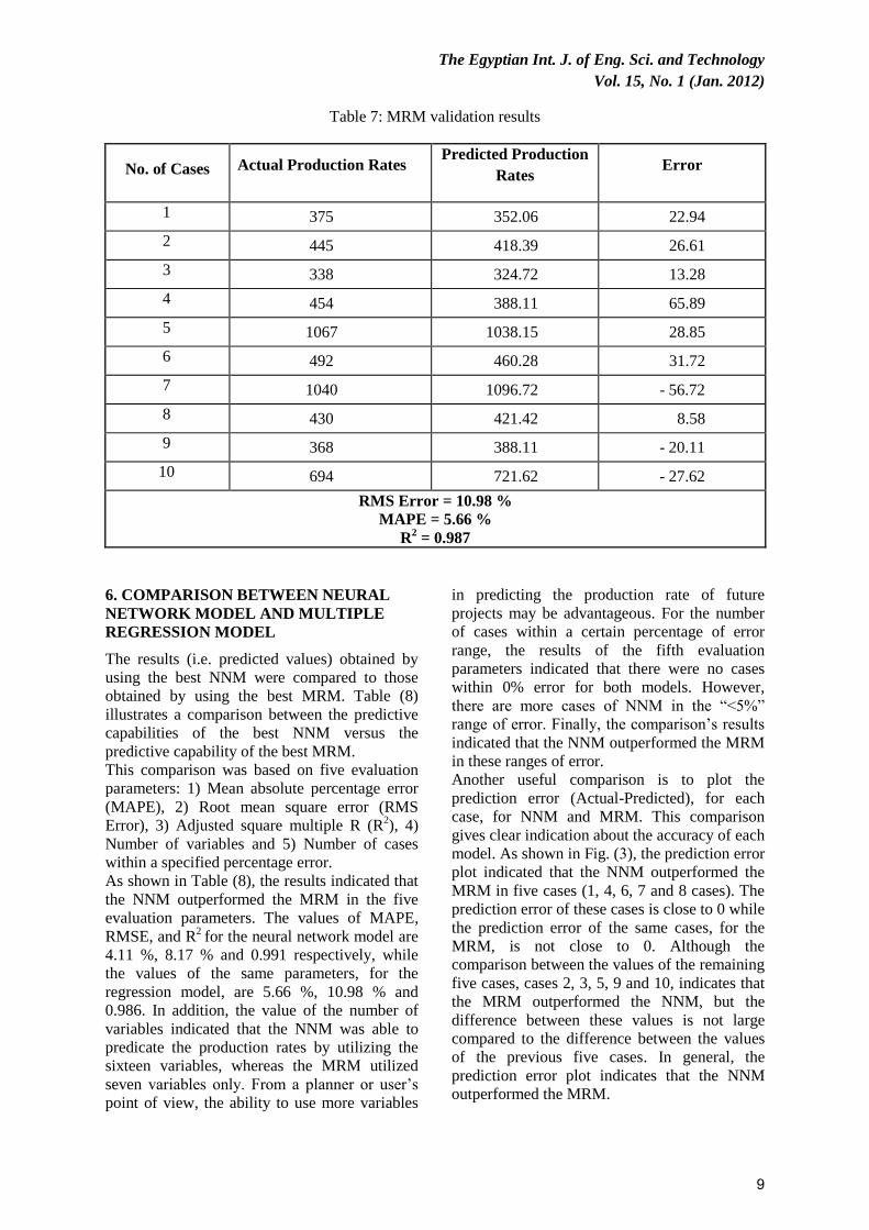
5.2 Regression Model Validation

The data, which were provided in the ten

validation sets, were applied to the equation (8).

The model produced ten predicted values for the

production rates of excavation operation. Three

evaluation parameters were used as the basis for

evaluating the performance of the MRM: (1) Root

mean square error (RMS Error); (2) Mean

absolute percentage error (MAPE); (3) adjusted

square multiple R (R2).

The results of the validation were tabulated in

Table (7). As shown in Table (7), the RMS Error,

MAPE and R2 were found to be 10.98 %, 5.66 %

and 0.986 respectively. These results reveal that

the developed model has excellent predictive capabilities.

8


Vol. 15, No. 1 (Jan. 2012)

Table 7: MRM validation results

No. of Cases Actual Production Rates Predicted Production

Rates Error

1 375 352.06 22.94

2 445 418.39 26.61

3 338 324.72 13.28

4 454 388.11 65.89

5 1067 1038.15 28.85

6 492 460.28 31.72

7 1040 1096.72 - 56.72

8 430 421.42 8.58

9 368 388.11 - 20.11

10 694 721.62 - 27.62

RMS Error = 10.98 %

MAPE = 5.66 %

R2 = 0.987

6. COMPARISON BETWEEN NEURAL

NETWORK MODEL AND MULTIPLE

REGRESSION MODEL

The results (i.e. predicted values) obtained by

using the best NNM were compared to those

obtained by using the best MRM. Table (8)

illustrates a comparison between the predictive

capabilities of the best NNM versus the

predictive capability of the best MRM.

This comparison was based on five evaluation

parameters: 1) Mean absolute percentage error

(MAPE), 2) Root mean square error (RMS

Error), 3) Adjusted square multiple R (R2), 4)

Number of variables and 5) Number of cases

within a specified percentage error.

As shown in Table (8), the results indicated that

the NNM outperformed the MRM in the five

evaluation parameters. The values of MAPE,

RMSE, and R2

for the neural network model are

4.11 %, 8.17 % and 0.991 respectively, while

the values of the same parameters, for the

regression model, are 5.66 %, 10.98 % and

0.986. In addition, the value of the number of

variables indicated that the NNM was able to

predicate the production rates by utilizing the

sixteen variables, whereas the MRM utilized

seven variables only. From a planner or user’s

point of view, the ability to use more variables

in predicting the production rate of future

projects may be advantageous. For the number

of cases within a certain percentage of error

range, the results of the fifth evaluation

parameters indicated that there were no cases

within 0% error for both models. However,

there are more cases of NNM in the “<5%”

range of error. Finally, the comparison’s results

indicated that the NNM outperformed the MRM

in these ranges of error.

Another useful comparison is to plot the

prediction error (Actual-Predicted), for each

case, for NNM and MRM. This comparison

gives clear indication about the accuracy of each

model. As shown in Fig. (3), the prediction error

plot indicated that the NNM outperformed the

MRM in five cases (1, 4, 6, 7 and 8 cases). The

prediction error of these cases is close to 0 while

the prediction error of the same cases, for the

MRM, is not close to 0. Although the

comparison between the values of the remaining

five cases, cases 2, 3, 5, 9 and 10, indicates that

the MRM outperformed the NNM, but the

difference between these values is not large

compared to the difference between the values

of the previous five cases. In general, the

prediction error plot indicates that the NNM

outperformed the MRM.

9



Table 8: Comparison between the NNM and MRM

Fig. 3. Prediction errors of NNM and MRM

7. CONCLUSIONS

This paper attempts to develop two NNM and

MRM that can be effectively used to predict the

production rate of excavation operation. Based

on a comprehensive review of literature and

interviews with project managers sixteen factors

were identified as the most significant factors

affecting the production rates of excavation

operation. A data collection form was designed

for collecting the data required. A total number

of eighty-five actual case studies were collected

from seventeen construction projects. It can be

concluded from the results of this study that:

1. The use of the NNM and MRM can help

estimators to reduce the effort required for

planning excavation operation as well as to

improve the accuracy of production rate

estimates to complete a project within budget

and schedule.

2. The results indicate that both NNM and

MRM can be effectively used to predict the

production rates of excavation operation.

However, the comparison between the

predictive capabilities of the best NNM versus

the predictive capabilities of the best MRM

indicates that the NNM outperformed the MRM.

10


Vol. 15, No. 1 (Jan. 2012)

REFERENCES

1. Attalla, M., Hegazy, T. and Haas, R., (2003),

“Reconstruction of the building infrastructure:

two performance prediction models.” J. Constr.

Eng. Manage., ASCE, Vol. 9 No 1, pp 26-34.

2. Bailey, D. and Thompson, D., (1990), “How to

develop neural network applications.” AI

Expert, Vol. 5 No 6, pp 38-47.

3. BrainMaker Professional -User’s Guide and

Reference Manual, (1998), California

Scientific Software.

4. Bhurisith, L., and Touran, A., (2002), “Case

study of obsolescence and equipment

productivity.” J. Constr. Eng. Manage., ASCE,

Vol. 128 No 4, pp 357-361.

5. Chao, L. and Skibniewski, M. J., (1994),

“Estimating construction productivity: Neural

network-based approach.” J. Comput. Civ.

Eng., ASCE, Vol. 8 No 2, pp 234-51.

6. Edwards, D. J and Holt, G. D., (2000),

“ESTIVATE: a model for calculating

excavator productivity and output costs.”

Engineering, Construction and Architectural

Management, Vol.1, pp 52-62.

7. Flood, I. and Christophilos, P., (1996),

“Modeling construction processes using

artificial neural networks.” Automation in

construction., Vol. 4 No 4, pp 307-320.

8. Hegazy, T. and Kassab, M., (2003), “Resource

optimization using combined simulation and

genetic algorithms.” J. Constr. Eng. Manage.,

ASCE, Vol. 129 No 6, pp 698-705.

9. Hegazy, T., Moselhi, O., and Fazio, P.,(1994),

“A neural network approach for representing

implicit knowledge in construction.” Int. J.

Constr. Inf. Technol., Vol.1 No. 3, pp 73-86.

10. Jonasson, S., Dunston, P. S., Ahmed, K., and

Hamilton, J., (2002), “Factors in productivity

and unit cost for advanced machine

guidance.” J. Constr. Eng. Manage., ASCE,

Vol. 128 No 5, pp 367-374.

11. Marzouk, M., and Moselhi, O., (2003),

“Object-oriented simulation model for

earthmoving operations.” J. Constr. Eng.

Manage., ASCE, Vol. 129 No 2, pp 173-181.

12. Marzouk, M. and Moselhi, O., (2004), “Fuzzy

clustering model for estimating haulers' travel

time.” J. Constr. Eng. Manage., ASCE, Vol.

130 No 6, pp 878-886.

13. Montgomery, D. C. and Runger, G. C., (2010),

Applied statistics and probability for

engineers. John Wiley & Sons, Inc.

14. Moselhi, O., (1991), "Neural networks as tools

in construction.” J. Constr. Eng. Manage.,

ASCE, Vol. 117 No 4, pp 606-625.

15. Moselhi, O., and Alshibani, A., (2009),

“optimization of earthmoving operations in

heavy civil engineering projects.” J. Constr.

Eng. Manage., ASCE, Vol. 135 No 10, pp

948 – 954.

16. Peurifoy, R. I. Schexnayder, C. J. and Shapira,

A., (2010), Construction planning equipment

and methods. Eighth Edition, Mc Graw-Hill

Companies, Inc., New York.

17. Rumelhart, D., Hinton, G., and Williams, R.,

(1986), Parallel distributed processing. Vol.1.

Foundations, MIT. Cambridge, Mass.

18. Shi, J. J., (1999), “A neural network based

system for predicting earthmoving

production.” Constr. Manage. Econom., Vol.

17, pp 463-471.

19. Smith, S.D., (1999), “Earthmoving

productivity estimation using linear

regression techniques.” J. Constr. Eng.

Manage., ASCE, Vol. 125 No 3, pp 133-141.

20. Tam, C.M., Tong, T. K.L. and Tse, S.L.,

(2002), “Artificial neural networks model for

predicting excavator productivity.” J. Eng.

Constr. Architect. Manage. Vol. 9 No 5-6,

pp 446-452.

21. Thabet, D. A., (2012), “Predicting of

production rate for excavation operation.”

PhD thesis, Faculty of Engineering, Zagazig

University, Zagazig, Egypt.

11

neural network and multiple regression models for

Documents