convolutional neural network models for axon segmentation...
TRANSCRIPT

Firma convenzione
Politecnico di Milano e Veneranda Fabbrica
del Duomo di Milano
Aula Magna ndash Rettorato
Mercoledigrave 27 maggio 2015
Convolutional neural network models
for axon segmentation in EM images
Advisor Elena DE MOMI PhD
Co-advisor Dott Ing Sara MOCCIA
Co-advisor Dott Ing Marco VIDOTTO
MSc Candidate Michele GAZZARA
Michele Gazzara 21122017
Clinical context - GBM
Glioblastoma multiforme (GBM) is the most common (50 of all cases) andthe most malignant (WHO Grade IV) of the glial cancers
Primary GBM without a clinical history
Secondary GBM originated from low grade tumors
Poor prognosis(12- 15 mo)
Pic adapted from [PY Wen et al 2008]
[P Kleihues et al 1999][M Eckley et al 2010]
[J C Buckner et al 2007]
(2)
Michele Gazzara 21122017
Clinical context - GBM treatment
Surgical resection Radiation therapy Chemotherapy
High GBM infiltration
Dose limitations
Blood Brain Barrier (BBB)
[F Hanif et al 2017][M Mrugala 2013]
(3)
Michele Gazzara 21122017
Clinical context - CED
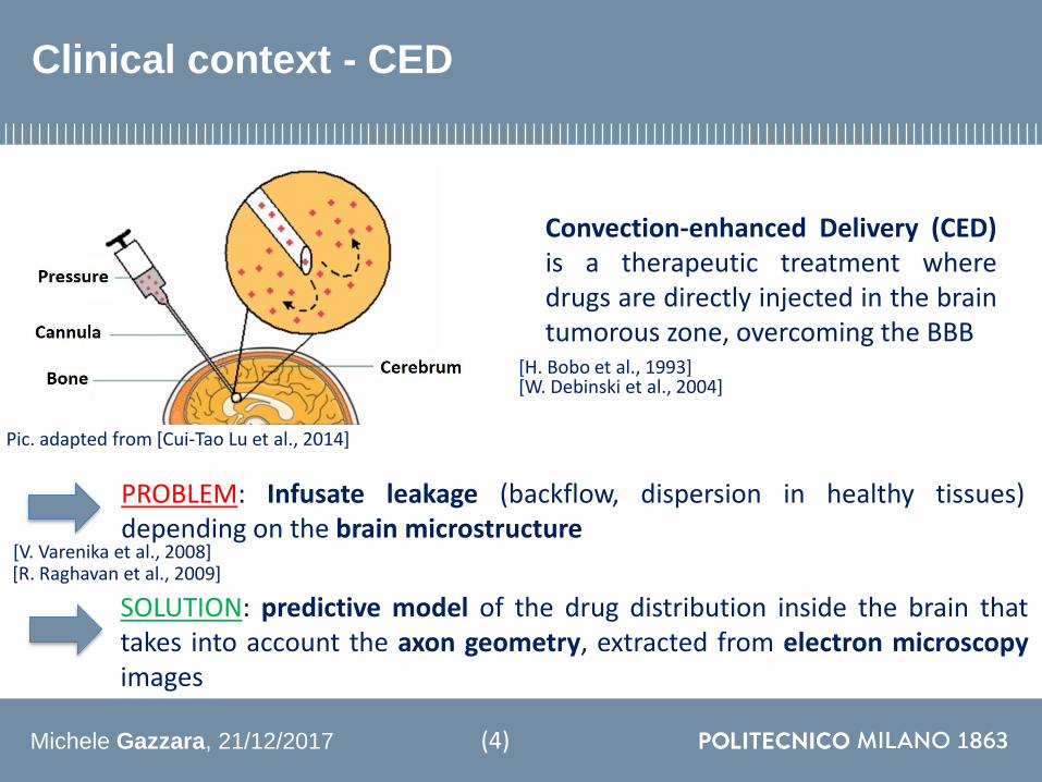
Convection-enhanced Delivery (CED)is a therapeutic treatment wheredrugs are directly injected in the braintumorous zone overcoming the BBB
PROBLEM Infusate leakage (backflow dispersion in healthy tissues)depending on the brain microstructure
SOLUTION predictive model of the drug distribution inside the brain thattakes into account the axon geometry extracted from electron microscopyimages
Pic adapted from [Cui-Tao Lu et al 2014]
[H Bobo et al 1993][W Debinski et al 2004]
[V Varenika et al 2008][R Raghavan et al 2009]
(4)
Michele Gazzara 21122017
Clinical context - EM imaging
Electron microscopy (EM) resolution ranges from nanometersdown to below an Aringngstroumlm
Scanning Electron Microscopy (SEM)
Transmission Electron Microscopy (TEM)Electron beam
Focusing lens
Sample
Electron beam
Focusing lens
Sample
[G Knott et al 2013][B Titze et al 2016]
Pic from [Liewald et al 2014] Pic from ISBI2012 Challenge dataset
(5)
Michele Gazzara 21122017
State of the art
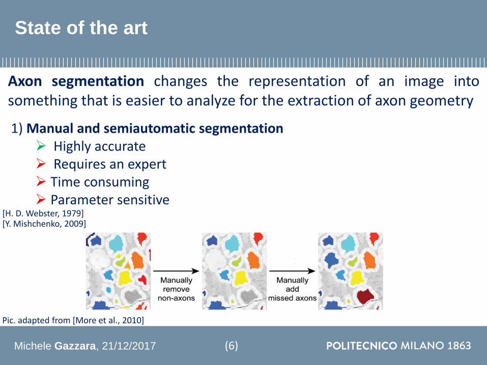
1) Manual and semiautomatic segmentation Highly accurate Requires an expert Time consuming Parameter sensitive
Axon segmentation changes the representation of an image intosomething that is easier to analyze for the extraction of axon geometry
[H D Webster 1979][Y Mishchenko 2009]
Pic adapted from [More et al 2010]
(6)
Michele Gazzara 21122017
State of the art
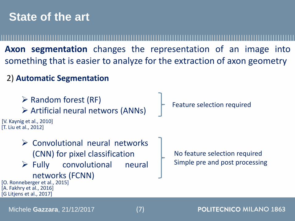
2) Automatic Segmentation
Random forest (RF) Artificial neural networs (ANNs)
Convolutional neural networks(CNN) for pixel classification
Fully convolutional neuralnetworks (FCNN)
Feature selection required
No feature selection requiredSimple pre and post processing
[V Kaynig et al 2010][T Liu et al 2012]
[O Ronneberger et al 2015]
[G Litjens et al 2017][A Fakhry et al 2016]
Axon segmentation changes the representation of an image intosomething that is easier to analyze for the extraction of axon geometry
(7)
Michele Gazzara 21122017
Thesis objective
The objective of this work is to develop Convolutional Neural Network(CNN) models for EM image segmentation
2 architectures are implementedArchitecture 1 CNN for binary pixel classificationArchitecture 2 Fully convolutional neural network (FCNN) for binary
image segmentation
(8)
Michele Gazzara 21122017
Thesis objective
The objective of this work is to develop Convolutional Neural Network(CNN) models for EM image segmentation
2 architectures are implementedArchitecture 1 CNN for binary pixel classificationArchitecture 2 Fully convolutional neural network (FCNN) for binary
image segmentation
2 hypotheses are investigatedH1 CNN approach exceeds in terms of accuracy the non CNN-based
methods and it is comparable with other existing CNN approachesH2 FCNN performances exceeds CNN ones in terms of accuracy and
computational costs
(8)
Michele Gazzara 21122017
Materials and methods
(9)
Michele Gazzara 21122017
Materials and methods - Patch extraction
(9)
Michele Gazzara 21122017
Patch extraction
DATASET ISBI2012 Challenge dataset was used for the network training (20 images) andtesting (10 images) 30 512 x 512 sections from a serial section Transmission Electron Microscopy (ssTEM)
data set of the Drosophila first instar larva ventral nerve cord The microcube measures 2 x 2 x 15 microns with a resolution of 4x4x50 nmpixel
327˙680patches
(10)
Architecture 1(65 x 65 patches)
Michele Gazzara 21122017
Patch extraction
1920patches
(10)
DATASET ISBI2012 Challenge dataset was used for the network training (20 images) andtesting (10 images) 30 512 x 512 sections from a serial section Transmission Electron Microscopy (ssTEM)
data set of the Drosophila first instar larva ventral nerve cord The microcube measures 2 x 2 x 15 microns with a resolution of 4x4x50 nmpixel
Architecture 2(256 x 256 patches)
Michele Gazzara 21122017
Materials and methods - CNN processing
(11)
Michele Gazzara 21122017
Architecture 1
Input patch65 x 65
Output pixel probability
(12)
Michele Gazzara 21122017
Architecture 1
CL-10 CL-3CL-3CL-5
Input patch65 x 65
Output pixel probability
CL-n nxn conv
(12)
Michele Gazzara 21122017 (13)
Convolutional layer
Michele Gazzara 21122017
Architecture 1
CL-10 CL-3CL-3CL-5
Input patch65 x 65
Output pixel probability
CL-n nxn conv
ReLUReLU ReLU
Michele Gazzara 21122017 (14)
Rectifying Linear Unit (ReLU)
ReLU (119909) = ቊ0 119894119891 119909 le 0119909 119894119891 119909 gt 0
Michele Gazzara 21122017
Architecture 1
CL-10 CL-3CL-3MPCL-5MP MP
Input patch65 x 65
Output pixel probability
CL-n nxn conv MP 2x2 max pool
ReLUReLU ReLU
Michele Gazzara 21122017 (15)
Max pooling layer
Michele Gazzara 21122017
Architecture 1
CL-10 CL-3CL-3MPCL-5MP MP FCFC SM
Input patch65 x 65
Output pixel probability
CL-n nxn conv MP 2x2 max pool FC Fully connected layer SM Softmax layer
ReLUReLU ReLU
Michele Gazzara 21122017 (16)
Fully connected and Softmax layers
As many FC output valuesas the number of classes
p119895 = 119890119911119895
σ119898=1119872 119890119911119898
j = 0 1 hellip M
Where119963119947 is the FC output
M is the number of classes
Michele Gazzara 21122017
Architecture 1
CL-10 CL-3CL-3MPCL-5MP MP FCFC SM
Input patch65 x 65
Output pixel probability
CL-n nxn conv MP 2x2 max pool FC Fully connected layer SM Softmax layer
ReLUReLU ReLU
Michele Gazzara 21122017
Architecture 2
Output patch probability map
216 x 216
Input patch
256 x 256
(17)
Michele Gazzara 21122017
Architecture 2
Output patch probability map
216 x 216
Input patch
256 x 256
(17)
Michele Gazzara 21122017 (18)
Up-convolution
1) Up-sampling
2) 2x2 convolution
[O Ronneberger et al 2015]
Michele Gazzara 21122017
Architecture 2
Output patch probability map
216 x 216
Input patch
256 x 256
Michele Gazzara 21122017
Training settings
Cross EntropyWhereN number of samplesi sample indexy sample labelp sample probability
J = minus1
119873σ119894=1119873 119910119894 119897119900119892 119901119894 + 1 minus 119910119894 ∙ 119897119900119892(1 minus 119901119894)
(19)
[D Kline et al 2005]
Michele Gazzara 21122017
Training settings
Cross EntropyWhereN number of samplesi sample indexy sample labelp sample probability
J = minus1
119873σ119894=1119873 119910119894 119897119900119892 119901119894 + 1 minus 119910119894 ∙ 119897119900119892(1 minus 119901119894)
Mini-batch gradient descent
θ = θ minus 120578 120571120579 119869 (120579 119909(119894119894+119899) 119901(119894119894+119899))
Where120520 learning raten batch sizex input sample
(19)
[D Kline et al 2005]
[M Li et al 2014]
Michele Gazzara 21122017
Training settings
Cross EntropyWhereN number of samplesi sample indexy sample labelp sample probability
J = minus1
119873σ119894=1119873 119910119894 119897119900119892 119901119894 + 1 minus 119910119894 ∙ 119897119900119892(1 minus 119901119894)
Mini-batch gradient descent
Adam Optimizer
θ = θ minus 120578 120571120579 119869 (120579 119909(119894119894+119899) 119901(119894119894+119899))
Where120520 learning raten batch sizex input sample
θ119905+1119896 = θ119905119896 minus120578
119907119905 119892119905119896 + 120598
∙ 119898119905(119892119905119896)
Wheret batch indexk node indexv uncentered variancem meang gradient of J
(19)
[D Kingma et al 2014]
[D Kline et al 2005]
[M Li et al 2014]
Michele Gazzara 21122017
Materials and methods - Post processing
(20)
Michele Gazzara 21122017
Post processing
Architecture 1
Pixel probability
Spatial imagereconstruction
Medianfiltering
Otsuthresholding
(21)
Michele Gazzara 21122017
Post processing
Architecture 1
Pixel probability
Spatial imagereconstruction
Medianfiltering
Otsuthresholding
(21)
Patch probability
map
Otsuthresholding
Architecture 2
Michele Gazzara 21122017
Materials and methods - Comparison
(22)
Michele Gazzara 21122017
Evaluation protocol - Metrics
Accuracy (Acc)
Pixel error (PE)
Sensitivity (Sn) and Specificity (Sp)
SoslashrensenndashDice coefficient (DSC)
Sn = TP
TP+FN
PE = 1 - Acc
119860119888119888 =1
Nσj=1N 119904119888119900119903119890119895 score = ൝
1 119894119891 yj= ොy1198950 119894119891 yj ne ොy119895
119863119878119862 =2 119879119875
119865119875 + 119865119873 + 2 119879119875
Sp = TN
TN+FP
Where
119962119946 sample label
ෝ119962119946 prediction
N number of samples
i semple index
TP true positives
FN false negatives
TN true negatives
FP false positives
(23)
[I Arganda-Carreras et al 2015]
Michele Gazzara 21122017
Evaluation protocol - H1 and H2
Investigation of H1
VSNon CNN-based approaches
CNN-based approaches
Architecture 1(PE)
(24)
Investigation of H2
Architecture 1(Performance metrics and
computational costs)
Architecture 2(Performance metrics and
computational costs)
VS(Lilliefors and Wilcoxon test)
Michele Gazzara 21122017
Results - Investigation of H1
Model Method PE [∙10minus3]
Architecture 1 CNN 88
Kaynig et al (2010) RF 157
Liu et al (2012) ANN 134
Model Training images Training time PE [∙10minus3]
Architecture 1 327680 5 hours 10 min 88
Ciresan et al (2012) 3 millions 85 hours 60
Fakhry et al (2015) 42 millions 30 hours 51
Comparison with non-CNN based models
Comparison with other CNN based models
(25)
PE = 1 - Acc
Michele Gazzara 21122017
Evaluation protocol - H1 and H2
Investigation of H1
VSNon CNN-based approaches
CNN-based approaches
Architecture 1(PE)
Investigation of H2
Architecture 1(Performance metrics and
computational costs)
Architecture 2(Performance metrics and
computational costs)
VS(Lilliefors and Wilcoxon test)
Michele Gazzara 21122017
Results - Investigation of H2 metrics
(26)
Michele Gazzara 21122017
Results - Investigation of H2 computational costs
(27)
Michele Gazzara 21122017
Results - Segmented images
Architecture 2 output
Architecture 1 output
Input image Ground truth
(28)
Michele Gazzara 21122017
Discussion
H1
1 Architecture 1 performances exceed the non CNN-based models
2 Architecture 1 performances are comparable with other CNN-based models
Reduced dataset and training time
(29)
Michele Gazzara 21122017
Discussion
H1
1 Architecture 1 performances exceed the non CNN-based models
2 Architecture 1 performances are comparable with other CNN-based models
Reduced dataset and training time
H2
1 Architecture 2 overcomes Architecture 1in terms of accuracy
2 Architecture 2 computational costs are lower than Architecture 1
Architecture 1detects more FPs
Architecture 2 can be used for real
time applications
(29)
Michele Gazzara 21122017
Conclusions and future work
CONCLUSIONS
Automatic method for axon segmentation in EM images
Performances comparable with existing CNN models
Reduced computational costs
(30)
Michele Gazzara 21122017
Conclusions and future work
CONCLUSIONS
Automatic method for axon segmentation in EM images
Performances comparable with existing CNN models
Reduced computational costs
FUTURE WORK
Larger dataset
Human brain EM images
Up-convolution improvement
(30)
[H Gao et al 2017]
Michele Gazzara 21122017
Acknowledgements
(31)
Michele Gazzara 21122017
Thank you for your attention
(32)

Michele Gazzara 21122017
Clinical context - GBM
Glioblastoma multiforme (GBM) is the most common (50 of all cases) andthe most malignant (WHO Grade IV) of the glial cancers
Primary GBM without a clinical history
Secondary GBM originated from low grade tumors
Poor prognosis(12- 15 mo)
Pic adapted from [PY Wen et al 2008]
[P Kleihues et al 1999][M Eckley et al 2010]
[J C Buckner et al 2007]
(2)
Michele Gazzara 21122017
Clinical context - GBM treatment
Surgical resection Radiation therapy Chemotherapy
High GBM infiltration
Dose limitations
Blood Brain Barrier (BBB)
[F Hanif et al 2017][M Mrugala 2013]
(3)
Michele Gazzara 21122017
Clinical context - CED
Convection-enhanced Delivery (CED)is a therapeutic treatment wheredrugs are directly injected in the braintumorous zone overcoming the BBB
PROBLEM Infusate leakage (backflow dispersion in healthy tissues)depending on the brain microstructure
SOLUTION predictive model of the drug distribution inside the brain thattakes into account the axon geometry extracted from electron microscopyimages
Pic adapted from [Cui-Tao Lu et al 2014]
[H Bobo et al 1993][W Debinski et al 2004]
[V Varenika et al 2008][R Raghavan et al 2009]
(4)
Michele Gazzara 21122017
Clinical context - EM imaging
Electron microscopy (EM) resolution ranges from nanometersdown to below an Aringngstroumlm
Scanning Electron Microscopy (SEM)
Transmission Electron Microscopy (TEM)Electron beam
Focusing lens
Sample
Electron beam
Focusing lens
Sample
[G Knott et al 2013][B Titze et al 2016]
Pic from [Liewald et al 2014] Pic from ISBI2012 Challenge dataset
(5)
Michele Gazzara 21122017
State of the art
1) Manual and semiautomatic segmentation Highly accurate Requires an expert Time consuming Parameter sensitive
Axon segmentation changes the representation of an image intosomething that is easier to analyze for the extraction of axon geometry
[H D Webster 1979][Y Mishchenko 2009]
Pic adapted from [More et al 2010]
(6)
Michele Gazzara 21122017
State of the art
2) Automatic Segmentation
Random forest (RF) Artificial neural networs (ANNs)
Convolutional neural networks(CNN) for pixel classification
Fully convolutional neuralnetworks (FCNN)
Feature selection required
No feature selection requiredSimple pre and post processing
[V Kaynig et al 2010][T Liu et al 2012]
[O Ronneberger et al 2015]
[G Litjens et al 2017][A Fakhry et al 2016]
Axon segmentation changes the representation of an image intosomething that is easier to analyze for the extraction of axon geometry
(7)
Michele Gazzara 21122017
Thesis objective
The objective of this work is to develop Convolutional Neural Network(CNN) models for EM image segmentation
2 architectures are implementedArchitecture 1 CNN for binary pixel classificationArchitecture 2 Fully convolutional neural network (FCNN) for binary
image segmentation
(8)
Michele Gazzara 21122017
Thesis objective
The objective of this work is to develop Convolutional Neural Network(CNN) models for EM image segmentation
2 architectures are implementedArchitecture 1 CNN for binary pixel classificationArchitecture 2 Fully convolutional neural network (FCNN) for binary
image segmentation
2 hypotheses are investigatedH1 CNN approach exceeds in terms of accuracy the non CNN-based
methods and it is comparable with other existing CNN approachesH2 FCNN performances exceeds CNN ones in terms of accuracy and
computational costs
(8)
Michele Gazzara 21122017
Materials and methods
(9)
Michele Gazzara 21122017
Materials and methods - Patch extraction
(9)
Michele Gazzara 21122017
Patch extraction
DATASET ISBI2012 Challenge dataset was used for the network training (20 images) andtesting (10 images) 30 512 x 512 sections from a serial section Transmission Electron Microscopy (ssTEM)
data set of the Drosophila first instar larva ventral nerve cord The microcube measures 2 x 2 x 15 microns with a resolution of 4x4x50 nmpixel
327˙680patches
(10)
Architecture 1(65 x 65 patches)
Michele Gazzara 21122017
Patch extraction
1920patches
(10)
DATASET ISBI2012 Challenge dataset was used for the network training (20 images) andtesting (10 images) 30 512 x 512 sections from a serial section Transmission Electron Microscopy (ssTEM)
data set of the Drosophila first instar larva ventral nerve cord The microcube measures 2 x 2 x 15 microns with a resolution of 4x4x50 nmpixel
Architecture 2(256 x 256 patches)
Michele Gazzara 21122017
Materials and methods - CNN processing
(11)
Michele Gazzara 21122017
Architecture 1
Input patch65 x 65
Output pixel probability
(12)
Michele Gazzara 21122017
Architecture 1
CL-10 CL-3CL-3CL-5
Input patch65 x 65
Output pixel probability
CL-n nxn conv
(12)
Michele Gazzara 21122017 (13)
Convolutional layer
Michele Gazzara 21122017
Architecture 1
CL-10 CL-3CL-3CL-5
Input patch65 x 65
Output pixel probability
CL-n nxn conv
ReLUReLU ReLU
Michele Gazzara 21122017 (14)
Rectifying Linear Unit (ReLU)
ReLU (119909) = ቊ0 119894119891 119909 le 0119909 119894119891 119909 gt 0
Michele Gazzara 21122017
Architecture 1
CL-10 CL-3CL-3MPCL-5MP MP
Input patch65 x 65
Output pixel probability
CL-n nxn conv MP 2x2 max pool
ReLUReLU ReLU
Michele Gazzara 21122017 (15)
Max pooling layer
Michele Gazzara 21122017
Architecture 1
CL-10 CL-3CL-3MPCL-5MP MP FCFC SM
Input patch65 x 65
Output pixel probability
CL-n nxn conv MP 2x2 max pool FC Fully connected layer SM Softmax layer
ReLUReLU ReLU
Michele Gazzara 21122017 (16)
Fully connected and Softmax layers
As many FC output valuesas the number of classes
p119895 = 119890119911119895
σ119898=1119872 119890119911119898
j = 0 1 hellip M
Where119963119947 is the FC output
M is the number of classes
Michele Gazzara 21122017
Architecture 1
CL-10 CL-3CL-3MPCL-5MP MP FCFC SM
Input patch65 x 65
Output pixel probability
CL-n nxn conv MP 2x2 max pool FC Fully connected layer SM Softmax layer
ReLUReLU ReLU
Michele Gazzara 21122017
Architecture 2
Output patch probability map
216 x 216
Input patch
256 x 256
(17)
Michele Gazzara 21122017
Architecture 2
Output patch probability map
216 x 216
Input patch
256 x 256
(17)
Michele Gazzara 21122017 (18)
Up-convolution
1) Up-sampling
2) 2x2 convolution
[O Ronneberger et al 2015]
Michele Gazzara 21122017
Architecture 2
Output patch probability map
216 x 216
Input patch
256 x 256
Michele Gazzara 21122017
Training settings
Cross EntropyWhereN number of samplesi sample indexy sample labelp sample probability
J = minus1
119873σ119894=1119873 119910119894 119897119900119892 119901119894 + 1 minus 119910119894 ∙ 119897119900119892(1 minus 119901119894)
(19)
[D Kline et al 2005]
Michele Gazzara 21122017
Training settings
Cross EntropyWhereN number of samplesi sample indexy sample labelp sample probability
J = minus1
119873σ119894=1119873 119910119894 119897119900119892 119901119894 + 1 minus 119910119894 ∙ 119897119900119892(1 minus 119901119894)
Mini-batch gradient descent
θ = θ minus 120578 120571120579 119869 (120579 119909(119894119894+119899) 119901(119894119894+119899))
Where120520 learning raten batch sizex input sample
(19)
[D Kline et al 2005]
[M Li et al 2014]
Michele Gazzara 21122017
Training settings
Cross EntropyWhereN number of samplesi sample indexy sample labelp sample probability
J = minus1
119873σ119894=1119873 119910119894 119897119900119892 119901119894 + 1 minus 119910119894 ∙ 119897119900119892(1 minus 119901119894)
Mini-batch gradient descent
Adam Optimizer
θ = θ minus 120578 120571120579 119869 (120579 119909(119894119894+119899) 119901(119894119894+119899))
Where120520 learning raten batch sizex input sample
θ119905+1119896 = θ119905119896 minus120578
119907119905 119892119905119896 + 120598
∙ 119898119905(119892119905119896)
Wheret batch indexk node indexv uncentered variancem meang gradient of J
(19)
[D Kingma et al 2014]
[D Kline et al 2005]
[M Li et al 2014]
Michele Gazzara 21122017
Materials and methods - Post processing
(20)
Michele Gazzara 21122017
Post processing
Architecture 1
Pixel probability
Spatial imagereconstruction
Medianfiltering
Otsuthresholding
(21)
Michele Gazzara 21122017
Post processing
Architecture 1
Pixel probability
Spatial imagereconstruction
Medianfiltering
Otsuthresholding
(21)
Patch probability
map
Otsuthresholding
Architecture 2
Michele Gazzara 21122017
Materials and methods - Comparison
(22)
Michele Gazzara 21122017
Evaluation protocol - Metrics
Accuracy (Acc)
Pixel error (PE)
Sensitivity (Sn) and Specificity (Sp)
SoslashrensenndashDice coefficient (DSC)
Sn = TP
TP+FN
PE = 1 - Acc
119860119888119888 =1
Nσj=1N 119904119888119900119903119890119895 score = ൝
1 119894119891 yj= ොy1198950 119894119891 yj ne ොy119895
119863119878119862 =2 119879119875
119865119875 + 119865119873 + 2 119879119875
Sp = TN
TN+FP
Where
119962119946 sample label
ෝ119962119946 prediction
N number of samples
i semple index
TP true positives
FN false negatives
TN true negatives
FP false positives
(23)
[I Arganda-Carreras et al 2015]
Michele Gazzara 21122017
Evaluation protocol - H1 and H2
Investigation of H1
VSNon CNN-based approaches
CNN-based approaches
Architecture 1(PE)
(24)
Investigation of H2
Architecture 1(Performance metrics and
computational costs)
Architecture 2(Performance metrics and
computational costs)
VS(Lilliefors and Wilcoxon test)
Michele Gazzara 21122017
Results - Investigation of H1
Model Method PE [∙10minus3]
Architecture 1 CNN 88
Kaynig et al (2010) RF 157
Liu et al (2012) ANN 134
Model Training images Training time PE [∙10minus3]
Architecture 1 327680 5 hours 10 min 88
Ciresan et al (2012) 3 millions 85 hours 60
Fakhry et al (2015) 42 millions 30 hours 51
Comparison with non-CNN based models
Comparison with other CNN based models
(25)
PE = 1 - Acc
Michele Gazzara 21122017
Evaluation protocol - H1 and H2
Investigation of H1
VSNon CNN-based approaches
CNN-based approaches
Architecture 1(PE)
Investigation of H2
Architecture 1(Performance metrics and
computational costs)
Architecture 2(Performance metrics and
computational costs)
VS(Lilliefors and Wilcoxon test)
Michele Gazzara 21122017
Results - Investigation of H2 metrics
(26)
Michele Gazzara 21122017
Results - Investigation of H2 computational costs
(27)
Michele Gazzara 21122017
Results - Segmented images
Architecture 2 output
Architecture 1 output
Input image Ground truth
(28)
Michele Gazzara 21122017
Discussion
H1
1 Architecture 1 performances exceed the non CNN-based models
2 Architecture 1 performances are comparable with other CNN-based models
Reduced dataset and training time
(29)
Michele Gazzara 21122017
Discussion
H1
1 Architecture 1 performances exceed the non CNN-based models
2 Architecture 1 performances are comparable with other CNN-based models
Reduced dataset and training time
H2
1 Architecture 2 overcomes Architecture 1in terms of accuracy
2 Architecture 2 computational costs are lower than Architecture 1
Architecture 1detects more FPs
Architecture 2 can be used for real
time applications
(29)
Michele Gazzara 21122017
Conclusions and future work
CONCLUSIONS
Automatic method for axon segmentation in EM images
Performances comparable with existing CNN models
Reduced computational costs
(30)
Michele Gazzara 21122017
Conclusions and future work
CONCLUSIONS
Automatic method for axon segmentation in EM images
Performances comparable with existing CNN models
Reduced computational costs
FUTURE WORK
Larger dataset
Human brain EM images
Up-convolution improvement
(30)
[H Gao et al 2017]
Michele Gazzara 21122017
Acknowledgements
(31)
Michele Gazzara 21122017
Thank you for your attention
(32)

Michele Gazzara 21122017
Clinical context - GBM treatment
Surgical resection Radiation therapy Chemotherapy
High GBM infiltration
Dose limitations
Blood Brain Barrier (BBB)
[F Hanif et al 2017][M Mrugala 2013]
(3)
Michele Gazzara 21122017
Clinical context - CED
Convection-enhanced Delivery (CED)is a therapeutic treatment wheredrugs are directly injected in the braintumorous zone overcoming the BBB
PROBLEM Infusate leakage (backflow dispersion in healthy tissues)depending on the brain microstructure
SOLUTION predictive model of the drug distribution inside the brain thattakes into account the axon geometry extracted from electron microscopyimages
Pic adapted from [Cui-Tao Lu et al 2014]
[H Bobo et al 1993][W Debinski et al 2004]
[V Varenika et al 2008][R Raghavan et al 2009]
(4)
Michele Gazzara 21122017
Clinical context - EM imaging
Electron microscopy (EM) resolution ranges from nanometersdown to below an Aringngstroumlm
Scanning Electron Microscopy (SEM)
Transmission Electron Microscopy (TEM)Electron beam
Focusing lens
Sample
Electron beam
Focusing lens
Sample
[G Knott et al 2013][B Titze et al 2016]
Pic from [Liewald et al 2014] Pic from ISBI2012 Challenge dataset
(5)
Michele Gazzara 21122017
State of the art
1) Manual and semiautomatic segmentation Highly accurate Requires an expert Time consuming Parameter sensitive
Axon segmentation changes the representation of an image intosomething that is easier to analyze for the extraction of axon geometry
[H D Webster 1979][Y Mishchenko 2009]
Pic adapted from [More et al 2010]
(6)
Michele Gazzara 21122017
State of the art
2) Automatic Segmentation
Random forest (RF) Artificial neural networs (ANNs)
Convolutional neural networks(CNN) for pixel classification
Fully convolutional neuralnetworks (FCNN)
Feature selection required
No feature selection requiredSimple pre and post processing
[V Kaynig et al 2010][T Liu et al 2012]
[O Ronneberger et al 2015]
[G Litjens et al 2017][A Fakhry et al 2016]
Axon segmentation changes the representation of an image intosomething that is easier to analyze for the extraction of axon geometry
(7)
Michele Gazzara 21122017
Thesis objective
The objective of this work is to develop Convolutional Neural Network(CNN) models for EM image segmentation
2 architectures are implementedArchitecture 1 CNN for binary pixel classificationArchitecture 2 Fully convolutional neural network (FCNN) for binary
image segmentation
(8)
Michele Gazzara 21122017
Thesis objective
The objective of this work is to develop Convolutional Neural Network(CNN) models for EM image segmentation
2 architectures are implementedArchitecture 1 CNN for binary pixel classificationArchitecture 2 Fully convolutional neural network (FCNN) for binary
image segmentation
2 hypotheses are investigatedH1 CNN approach exceeds in terms of accuracy the non CNN-based
methods and it is comparable with other existing CNN approachesH2 FCNN performances exceeds CNN ones in terms of accuracy and
computational costs
(8)
Michele Gazzara 21122017
Materials and methods
(9)
Michele Gazzara 21122017
Materials and methods - Patch extraction
(9)
Michele Gazzara 21122017
Patch extraction
DATASET ISBI2012 Challenge dataset was used for the network training (20 images) andtesting (10 images) 30 512 x 512 sections from a serial section Transmission Electron Microscopy (ssTEM)
data set of the Drosophila first instar larva ventral nerve cord The microcube measures 2 x 2 x 15 microns with a resolution of 4x4x50 nmpixel
327˙680patches
(10)
Architecture 1(65 x 65 patches)
Michele Gazzara 21122017
Patch extraction
1920patches
(10)
DATASET ISBI2012 Challenge dataset was used for the network training (20 images) andtesting (10 images) 30 512 x 512 sections from a serial section Transmission Electron Microscopy (ssTEM)
data set of the Drosophila first instar larva ventral nerve cord The microcube measures 2 x 2 x 15 microns with a resolution of 4x4x50 nmpixel
Architecture 2(256 x 256 patches)
Michele Gazzara 21122017
Materials and methods - CNN processing
(11)
Michele Gazzara 21122017
Architecture 1
Input patch65 x 65
Output pixel probability
(12)
Michele Gazzara 21122017
Architecture 1
CL-10 CL-3CL-3CL-5
Input patch65 x 65
Output pixel probability
CL-n nxn conv
(12)
Michele Gazzara 21122017 (13)
Convolutional layer
Michele Gazzara 21122017
Architecture 1
CL-10 CL-3CL-3CL-5
Input patch65 x 65
Output pixel probability
CL-n nxn conv
ReLUReLU ReLU
Michele Gazzara 21122017 (14)
Rectifying Linear Unit (ReLU)
ReLU (119909) = ቊ0 119894119891 119909 le 0119909 119894119891 119909 gt 0
Michele Gazzara 21122017
Architecture 1
CL-10 CL-3CL-3MPCL-5MP MP
Input patch65 x 65
Output pixel probability
CL-n nxn conv MP 2x2 max pool
ReLUReLU ReLU
Michele Gazzara 21122017 (15)
Max pooling layer
Michele Gazzara 21122017
Architecture 1
CL-10 CL-3CL-3MPCL-5MP MP FCFC SM
Input patch65 x 65
Output pixel probability
CL-n nxn conv MP 2x2 max pool FC Fully connected layer SM Softmax layer
ReLUReLU ReLU
Michele Gazzara 21122017 (16)
Fully connected and Softmax layers
As many FC output valuesas the number of classes
p119895 = 119890119911119895
σ119898=1119872 119890119911119898
j = 0 1 hellip M
Where119963119947 is the FC output
M is the number of classes
Michele Gazzara 21122017
Architecture 1
CL-10 CL-3CL-3MPCL-5MP MP FCFC SM
Input patch65 x 65
Output pixel probability
CL-n nxn conv MP 2x2 max pool FC Fully connected layer SM Softmax layer
ReLUReLU ReLU
Michele Gazzara 21122017
Architecture 2
Output patch probability map
216 x 216
Input patch
256 x 256
(17)
Michele Gazzara 21122017
Architecture 2
Output patch probability map
216 x 216
Input patch
256 x 256
(17)
Michele Gazzara 21122017 (18)
Up-convolution
1) Up-sampling
2) 2x2 convolution
[O Ronneberger et al 2015]
Michele Gazzara 21122017
Architecture 2
Output patch probability map
216 x 216
Input patch
256 x 256
Michele Gazzara 21122017
Training settings
Cross EntropyWhereN number of samplesi sample indexy sample labelp sample probability
J = minus1
119873σ119894=1119873 119910119894 119897119900119892 119901119894 + 1 minus 119910119894 ∙ 119897119900119892(1 minus 119901119894)
(19)
[D Kline et al 2005]
Michele Gazzara 21122017
Training settings
Cross EntropyWhereN number of samplesi sample indexy sample labelp sample probability
J = minus1
119873σ119894=1119873 119910119894 119897119900119892 119901119894 + 1 minus 119910119894 ∙ 119897119900119892(1 minus 119901119894)
Mini-batch gradient descent
θ = θ minus 120578 120571120579 119869 (120579 119909(119894119894+119899) 119901(119894119894+119899))
Where120520 learning raten batch sizex input sample
(19)
[D Kline et al 2005]
[M Li et al 2014]
Michele Gazzara 21122017
Training settings
Cross EntropyWhereN number of samplesi sample indexy sample labelp sample probability
J = minus1
119873σ119894=1119873 119910119894 119897119900119892 119901119894 + 1 minus 119910119894 ∙ 119897119900119892(1 minus 119901119894)
Mini-batch gradient descent
Adam Optimizer
θ = θ minus 120578 120571120579 119869 (120579 119909(119894119894+119899) 119901(119894119894+119899))
Where120520 learning raten batch sizex input sample
θ119905+1119896 = θ119905119896 minus120578
119907119905 119892119905119896 + 120598
∙ 119898119905(119892119905119896)
Wheret batch indexk node indexv uncentered variancem meang gradient of J
(19)
[D Kingma et al 2014]
[D Kline et al 2005]
[M Li et al 2014]
Michele Gazzara 21122017
Materials and methods - Post processing
(20)
Michele Gazzara 21122017
Post processing
Architecture 1
Pixel probability
Spatial imagereconstruction
Medianfiltering
Otsuthresholding
(21)
Michele Gazzara 21122017
Post processing
Architecture 1
Pixel probability
Spatial imagereconstruction
Medianfiltering
Otsuthresholding
(21)
Patch probability
map
Otsuthresholding
Architecture 2
Michele Gazzara 21122017
Materials and methods - Comparison
(22)
Michele Gazzara 21122017
Evaluation protocol - Metrics
Accuracy (Acc)
Pixel error (PE)
Sensitivity (Sn) and Specificity (Sp)
SoslashrensenndashDice coefficient (DSC)
Sn = TP
TP+FN
PE = 1 - Acc
119860119888119888 =1
Nσj=1N 119904119888119900119903119890119895 score = ൝
1 119894119891 yj= ොy1198950 119894119891 yj ne ොy119895
119863119878119862 =2 119879119875
119865119875 + 119865119873 + 2 119879119875
Sp = TN
TN+FP
Where
119962119946 sample label
ෝ119962119946 prediction
N number of samples
i semple index
TP true positives
FN false negatives
TN true negatives
FP false positives
(23)
[I Arganda-Carreras et al 2015]
Michele Gazzara 21122017
Evaluation protocol - H1 and H2
Investigation of H1
VSNon CNN-based approaches
CNN-based approaches
Architecture 1(PE)
(24)
Investigation of H2
Architecture 1(Performance metrics and
computational costs)
Architecture 2(Performance metrics and
computational costs)
VS(Lilliefors and Wilcoxon test)
Michele Gazzara 21122017
Results - Investigation of H1
Model Method PE [∙10minus3]
Architecture 1 CNN 88
Kaynig et al (2010) RF 157
Liu et al (2012) ANN 134
Model Training images Training time PE [∙10minus3]
Architecture 1 327680 5 hours 10 min 88
Ciresan et al (2012) 3 millions 85 hours 60
Fakhry et al (2015) 42 millions 30 hours 51
Comparison with non-CNN based models
Comparison with other CNN based models
(25)
PE = 1 - Acc
Michele Gazzara 21122017
Evaluation protocol - H1 and H2
Investigation of H1
VSNon CNN-based approaches
CNN-based approaches
Architecture 1(PE)
Investigation of H2
Architecture 1(Performance metrics and
computational costs)
Architecture 2(Performance metrics and
computational costs)
VS(Lilliefors and Wilcoxon test)
Michele Gazzara 21122017
Results - Investigation of H2 metrics
(26)
Michele Gazzara 21122017
Results - Investigation of H2 computational costs
(27)
Michele Gazzara 21122017
Results - Segmented images
Architecture 2 output
Architecture 1 output
Input image Ground truth
(28)
Michele Gazzara 21122017
Discussion
H1
1 Architecture 1 performances exceed the non CNN-based models
2 Architecture 1 performances are comparable with other CNN-based models
Reduced dataset and training time
(29)
Michele Gazzara 21122017
Discussion
H1
1 Architecture 1 performances exceed the non CNN-based models
2 Architecture 1 performances are comparable with other CNN-based models
Reduced dataset and training time
H2
1 Architecture 2 overcomes Architecture 1in terms of accuracy
2 Architecture 2 computational costs are lower than Architecture 1
Architecture 1detects more FPs
Architecture 2 can be used for real
time applications
(29)
Michele Gazzara 21122017
Conclusions and future work
CONCLUSIONS
Automatic method for axon segmentation in EM images
Performances comparable with existing CNN models
Reduced computational costs
(30)
Michele Gazzara 21122017
Conclusions and future work
CONCLUSIONS
Automatic method for axon segmentation in EM images
Performances comparable with existing CNN models
Reduced computational costs
FUTURE WORK
Larger dataset
Human brain EM images
Up-convolution improvement
(30)
[H Gao et al 2017]
Michele Gazzara 21122017
Acknowledgements
(31)
Michele Gazzara 21122017
Thank you for your attention
(32)
Michele Gazzara 21122017
Clinical context - CED
Convection-enhanced Delivery (CED)is a therapeutic treatment wheredrugs are directly injected in the braintumorous zone overcoming the BBB
PROBLEM Infusate leakage (backflow dispersion in healthy tissues)depending on the brain microstructure
SOLUTION predictive model of the drug distribution inside the brain thattakes into account the axon geometry extracted from electron microscopyimages
Pic adapted from [Cui-Tao Lu et al 2014]
[H Bobo et al 1993][W Debinski et al 2004]
[V Varenika et al 2008][R Raghavan et al 2009]
(4)
Michele Gazzara 21122017
Clinical context - EM imaging
Electron microscopy (EM) resolution ranges from nanometersdown to below an Aringngstroumlm
Scanning Electron Microscopy (SEM)
Transmission Electron Microscopy (TEM)Electron beam
Focusing lens
Sample
Electron beam
Focusing lens
Sample
[G Knott et al 2013][B Titze et al 2016]
Pic from [Liewald et al 2014] Pic from ISBI2012 Challenge dataset
(5)
Michele Gazzara 21122017
State of the art
1) Manual and semiautomatic segmentation Highly accurate Requires an expert Time consuming Parameter sensitive
Axon segmentation changes the representation of an image intosomething that is easier to analyze for the extraction of axon geometry
[H D Webster 1979][Y Mishchenko 2009]
Pic adapted from [More et al 2010]
(6)
Michele Gazzara 21122017
State of the art
2) Automatic Segmentation
Random forest (RF) Artificial neural networs (ANNs)
Convolutional neural networks(CNN) for pixel classification
Fully convolutional neuralnetworks (FCNN)
Feature selection required
No feature selection requiredSimple pre and post processing
[V Kaynig et al 2010][T Liu et al 2012]
[O Ronneberger et al 2015]
[G Litjens et al 2017][A Fakhry et al 2016]
Axon segmentation changes the representation of an image intosomething that is easier to analyze for the extraction of axon geometry
(7)
Michele Gazzara 21122017
Thesis objective
The objective of this work is to develop Convolutional Neural Network(CNN) models for EM image segmentation
2 architectures are implementedArchitecture 1 CNN for binary pixel classificationArchitecture 2 Fully convolutional neural network (FCNN) for binary
image segmentation
(8)
Michele Gazzara 21122017
Thesis objective
The objective of this work is to develop Convolutional Neural Network(CNN) models for EM image segmentation
2 architectures are implementedArchitecture 1 CNN for binary pixel classificationArchitecture 2 Fully convolutional neural network (FCNN) for binary
image segmentation
2 hypotheses are investigatedH1 CNN approach exceeds in terms of accuracy the non CNN-based
methods and it is comparable with other existing CNN approachesH2 FCNN performances exceeds CNN ones in terms of accuracy and
computational costs
(8)
Michele Gazzara 21122017
Materials and methods
(9)
Michele Gazzara 21122017
Materials and methods - Patch extraction
(9)
Michele Gazzara 21122017
Patch extraction
DATASET ISBI2012 Challenge dataset was used for the network training (20 images) andtesting (10 images) 30 512 x 512 sections from a serial section Transmission Electron Microscopy (ssTEM)
data set of the Drosophila first instar larva ventral nerve cord The microcube measures 2 x 2 x 15 microns with a resolution of 4x4x50 nmpixel
327˙680patches
(10)
Architecture 1(65 x 65 patches)
Michele Gazzara 21122017
Patch extraction
1920patches
(10)
DATASET ISBI2012 Challenge dataset was used for the network training (20 images) andtesting (10 images) 30 512 x 512 sections from a serial section Transmission Electron Microscopy (ssTEM)
data set of the Drosophila first instar larva ventral nerve cord The microcube measures 2 x 2 x 15 microns with a resolution of 4x4x50 nmpixel
Architecture 2(256 x 256 patches)
Michele Gazzara 21122017
Materials and methods - CNN processing
(11)
Michele Gazzara 21122017
Architecture 1
Input patch65 x 65
Output pixel probability
(12)
Michele Gazzara 21122017
Architecture 1
CL-10 CL-3CL-3CL-5
Input patch65 x 65
Output pixel probability
CL-n nxn conv
(12)
Michele Gazzara 21122017 (13)
Convolutional layer
Michele Gazzara 21122017
Architecture 1
CL-10 CL-3CL-3CL-5
Input patch65 x 65
Output pixel probability
CL-n nxn conv
ReLUReLU ReLU
Michele Gazzara 21122017 (14)
Rectifying Linear Unit (ReLU)
ReLU (119909) = ቊ0 119894119891 119909 le 0119909 119894119891 119909 gt 0
Michele Gazzara 21122017
Architecture 1
CL-10 CL-3CL-3MPCL-5MP MP
Input patch65 x 65
Output pixel probability
CL-n nxn conv MP 2x2 max pool
ReLUReLU ReLU
Michele Gazzara 21122017 (15)
Max pooling layer
Michele Gazzara 21122017
Architecture 1
CL-10 CL-3CL-3MPCL-5MP MP FCFC SM
Input patch65 x 65
Output pixel probability
CL-n nxn conv MP 2x2 max pool FC Fully connected layer SM Softmax layer
ReLUReLU ReLU
Michele Gazzara 21122017 (16)
Fully connected and Softmax layers
As many FC output valuesas the number of classes
p119895 = 119890119911119895
σ119898=1119872 119890119911119898
j = 0 1 hellip M
Where119963119947 is the FC output
M is the number of classes
Michele Gazzara 21122017
Architecture 1
CL-10 CL-3CL-3MPCL-5MP MP FCFC SM
Input patch65 x 65
Output pixel probability
CL-n nxn conv MP 2x2 max pool FC Fully connected layer SM Softmax layer
ReLUReLU ReLU
Michele Gazzara 21122017
Architecture 2
Output patch probability map
216 x 216
Input patch
256 x 256
(17)
Michele Gazzara 21122017
Architecture 2
Output patch probability map
216 x 216
Input patch
256 x 256
(17)
Michele Gazzara 21122017 (18)
Up-convolution
1) Up-sampling
2) 2x2 convolution
[O Ronneberger et al 2015]
Michele Gazzara 21122017
Architecture 2
Output patch probability map
216 x 216
Input patch
256 x 256
Michele Gazzara 21122017
Training settings
Cross EntropyWhereN number of samplesi sample indexy sample labelp sample probability
J = minus1
119873σ119894=1119873 119910119894 119897119900119892 119901119894 + 1 minus 119910119894 ∙ 119897119900119892(1 minus 119901119894)
(19)
[D Kline et al 2005]
Michele Gazzara 21122017
Training settings
Cross EntropyWhereN number of samplesi sample indexy sample labelp sample probability
J = minus1
119873σ119894=1119873 119910119894 119897119900119892 119901119894 + 1 minus 119910119894 ∙ 119897119900119892(1 minus 119901119894)
Mini-batch gradient descent
θ = θ minus 120578 120571120579 119869 (120579 119909(119894119894+119899) 119901(119894119894+119899))
Where120520 learning raten batch sizex input sample
(19)
[D Kline et al 2005]
[M Li et al 2014]
Michele Gazzara 21122017
Training settings
Cross EntropyWhereN number of samplesi sample indexy sample labelp sample probability
J = minus1
119873σ119894=1119873 119910119894 119897119900119892 119901119894 + 1 minus 119910119894 ∙ 119897119900119892(1 minus 119901119894)
Mini-batch gradient descent
Adam Optimizer
θ = θ minus 120578 120571120579 119869 (120579 119909(119894119894+119899) 119901(119894119894+119899))
Where120520 learning raten batch sizex input sample
θ119905+1119896 = θ119905119896 minus120578
119907119905 119892119905119896 + 120598
∙ 119898119905(119892119905119896)
Wheret batch indexk node indexv uncentered variancem meang gradient of J
(19)
[D Kingma et al 2014]
[D Kline et al 2005]
[M Li et al 2014]
Michele Gazzara 21122017
Materials and methods - Post processing
(20)
Michele Gazzara 21122017
Post processing
Architecture 1
Pixel probability
Spatial imagereconstruction
Medianfiltering
Otsuthresholding
(21)
Michele Gazzara 21122017
Post processing
Architecture 1
Pixel probability
Spatial imagereconstruction
Medianfiltering
Otsuthresholding
(21)
Patch probability
map
Otsuthresholding
Architecture 2
Michele Gazzara 21122017
Materials and methods - Comparison
(22)
Michele Gazzara 21122017
Evaluation protocol - Metrics
Accuracy (Acc)
Pixel error (PE)
Sensitivity (Sn) and Specificity (Sp)
SoslashrensenndashDice coefficient (DSC)
Sn = TP
TP+FN
PE = 1 - Acc
119860119888119888 =1
Nσj=1N 119904119888119900119903119890119895 score = ൝
1 119894119891 yj= ොy1198950 119894119891 yj ne ොy119895
119863119878119862 =2 119879119875
119865119875 + 119865119873 + 2 119879119875
Sp = TN
TN+FP
Where
119962119946 sample label
ෝ119962119946 prediction
N number of samples
i semple index
TP true positives
FN false negatives
TN true negatives
FP false positives
(23)
[I Arganda-Carreras et al 2015]
Michele Gazzara 21122017
Evaluation protocol - H1 and H2
Investigation of H1
VSNon CNN-based approaches
CNN-based approaches
Architecture 1(PE)
(24)
Investigation of H2
Architecture 1(Performance metrics and
computational costs)
Architecture 2(Performance metrics and
computational costs)
VS(Lilliefors and Wilcoxon test)
Michele Gazzara 21122017
Results - Investigation of H1
Model Method PE [∙10minus3]
Architecture 1 CNN 88
Kaynig et al (2010) RF 157
Liu et al (2012) ANN 134
Model Training images Training time PE [∙10minus3]
Architecture 1 327680 5 hours 10 min 88
Ciresan et al (2012) 3 millions 85 hours 60
Fakhry et al (2015) 42 millions 30 hours 51
Comparison with non-CNN based models
Comparison with other CNN based models
(25)
PE = 1 - Acc
Michele Gazzara 21122017
Evaluation protocol - H1 and H2
Investigation of H1
VSNon CNN-based approaches
CNN-based approaches
Architecture 1(PE)
Investigation of H2
Architecture 1(Performance metrics and
computational costs)
Architecture 2(Performance metrics and
computational costs)
VS(Lilliefors and Wilcoxon test)
Michele Gazzara 21122017
Results - Investigation of H2 metrics
(26)
Michele Gazzara 21122017
Results - Investigation of H2 computational costs
(27)
Michele Gazzara 21122017
Results - Segmented images
Architecture 2 output
Architecture 1 output
Input image Ground truth
(28)
Michele Gazzara 21122017
Discussion
H1
1 Architecture 1 performances exceed the non CNN-based models
2 Architecture 1 performances are comparable with other CNN-based models
Reduced dataset and training time
(29)
Michele Gazzara 21122017
Discussion
H1
1 Architecture 1 performances exceed the non CNN-based models
2 Architecture 1 performances are comparable with other CNN-based models
Reduced dataset and training time
H2
1 Architecture 2 overcomes Architecture 1in terms of accuracy
2 Architecture 2 computational costs are lower than Architecture 1
Architecture 1detects more FPs
Architecture 2 can be used for real
time applications
(29)
Michele Gazzara 21122017
Conclusions and future work
CONCLUSIONS
Automatic method for axon segmentation in EM images
Performances comparable with existing CNN models
Reduced computational costs
(30)
Michele Gazzara 21122017
Conclusions and future work
CONCLUSIONS
Automatic method for axon segmentation in EM images
Performances comparable with existing CNN models
Reduced computational costs
FUTURE WORK
Larger dataset
Human brain EM images
Up-convolution improvement
(30)
[H Gao et al 2017]
Michele Gazzara 21122017
Acknowledgements
(31)
Michele Gazzara 21122017
Thank you for your attention
(32)

Michele Gazzara 21122017
Clinical context - EM imaging
Electron microscopy (EM) resolution ranges from nanometersdown to below an Aringngstroumlm
Scanning Electron Microscopy (SEM)
Transmission Electron Microscopy (TEM)Electron beam
Focusing lens
Sample
Electron beam
Focusing lens
Sample
[G Knott et al 2013][B Titze et al 2016]
Pic from [Liewald et al 2014] Pic from ISBI2012 Challenge dataset
(5)
Michele Gazzara 21122017
State of the art
1) Manual and semiautomatic segmentation Highly accurate Requires an expert Time consuming Parameter sensitive
Axon segmentation changes the representation of an image intosomething that is easier to analyze for the extraction of axon geometry
[H D Webster 1979][Y Mishchenko 2009]
Pic adapted from [More et al 2010]
(6)
Michele Gazzara 21122017
State of the art
2) Automatic Segmentation
Random forest (RF) Artificial neural networs (ANNs)
Convolutional neural networks(CNN) for pixel classification
Fully convolutional neuralnetworks (FCNN)
Feature selection required
No feature selection requiredSimple pre and post processing
[V Kaynig et al 2010][T Liu et al 2012]
[O Ronneberger et al 2015]
[G Litjens et al 2017][A Fakhry et al 2016]
Axon segmentation changes the representation of an image intosomething that is easier to analyze for the extraction of axon geometry
(7)
Michele Gazzara 21122017
Thesis objective
The objective of this work is to develop Convolutional Neural Network(CNN) models for EM image segmentation
2 architectures are implementedArchitecture 1 CNN for binary pixel classificationArchitecture 2 Fully convolutional neural network (FCNN) for binary
image segmentation
(8)
Michele Gazzara 21122017
Thesis objective
The objective of this work is to develop Convolutional Neural Network(CNN) models for EM image segmentation
2 architectures are implementedArchitecture 1 CNN for binary pixel classificationArchitecture 2 Fully convolutional neural network (FCNN) for binary
image segmentation
2 hypotheses are investigatedH1 CNN approach exceeds in terms of accuracy the non CNN-based
methods and it is comparable with other existing CNN approachesH2 FCNN performances exceeds CNN ones in terms of accuracy and
computational costs
(8)
Michele Gazzara 21122017
Materials and methods
(9)
Michele Gazzara 21122017
Materials and methods - Patch extraction
(9)
Michele Gazzara 21122017
Patch extraction
DATASET ISBI2012 Challenge dataset was used for the network training (20 images) andtesting (10 images) 30 512 x 512 sections from a serial section Transmission Electron Microscopy (ssTEM)
data set of the Drosophila first instar larva ventral nerve cord The microcube measures 2 x 2 x 15 microns with a resolution of 4x4x50 nmpixel
327˙680patches
(10)
Architecture 1(65 x 65 patches)
Michele Gazzara 21122017
Patch extraction
1920patches
(10)
DATASET ISBI2012 Challenge dataset was used for the network training (20 images) andtesting (10 images) 30 512 x 512 sections from a serial section Transmission Electron Microscopy (ssTEM)
data set of the Drosophila first instar larva ventral nerve cord The microcube measures 2 x 2 x 15 microns with a resolution of 4x4x50 nmpixel
Architecture 2(256 x 256 patches)
Michele Gazzara 21122017
Materials and methods - CNN processing
(11)
Michele Gazzara 21122017
Architecture 1
Input patch65 x 65
Output pixel probability
(12)
Michele Gazzara 21122017
Architecture 1
CL-10 CL-3CL-3CL-5
Input patch65 x 65
Output pixel probability
CL-n nxn conv
(12)
Michele Gazzara 21122017 (13)
Convolutional layer
Michele Gazzara 21122017
Architecture 1
CL-10 CL-3CL-3CL-5
Input patch65 x 65
Output pixel probability
CL-n nxn conv
ReLUReLU ReLU
Michele Gazzara 21122017 (14)
Rectifying Linear Unit (ReLU)
ReLU (119909) = ቊ0 119894119891 119909 le 0119909 119894119891 119909 gt 0
Michele Gazzara 21122017
Architecture 1
CL-10 CL-3CL-3MPCL-5MP MP
Input patch65 x 65
Output pixel probability
CL-n nxn conv MP 2x2 max pool
ReLUReLU ReLU
Michele Gazzara 21122017 (15)
Max pooling layer
Michele Gazzara 21122017
Architecture 1
CL-10 CL-3CL-3MPCL-5MP MP FCFC SM
Input patch65 x 65
Output pixel probability
CL-n nxn conv MP 2x2 max pool FC Fully connected layer SM Softmax layer
ReLUReLU ReLU
Michele Gazzara 21122017 (16)
Fully connected and Softmax layers
As many FC output valuesas the number of classes
p119895 = 119890119911119895
σ119898=1119872 119890119911119898
j = 0 1 hellip M
Where119963119947 is the FC output
M is the number of classes
Michele Gazzara 21122017
Architecture 1
CL-10 CL-3CL-3MPCL-5MP MP FCFC SM
Input patch65 x 65
Output pixel probability
CL-n nxn conv MP 2x2 max pool FC Fully connected layer SM Softmax layer
ReLUReLU ReLU
Michele Gazzara 21122017
Architecture 2
Output patch probability map
216 x 216
Input patch
256 x 256
(17)
Michele Gazzara 21122017
Architecture 2
Output patch probability map
216 x 216
Input patch
256 x 256
(17)
Michele Gazzara 21122017 (18)
Up-convolution
1) Up-sampling
2) 2x2 convolution
[O Ronneberger et al 2015]
Michele Gazzara 21122017
Architecture 2
Output patch probability map
216 x 216
Input patch
256 x 256
Michele Gazzara 21122017
Training settings
Cross EntropyWhereN number of samplesi sample indexy sample labelp sample probability
J = minus1
119873σ119894=1119873 119910119894 119897119900119892 119901119894 + 1 minus 119910119894 ∙ 119897119900119892(1 minus 119901119894)
(19)
[D Kline et al 2005]
Michele Gazzara 21122017
Training settings
Cross EntropyWhereN number of samplesi sample indexy sample labelp sample probability
J = minus1
119873σ119894=1119873 119910119894 119897119900119892 119901119894 + 1 minus 119910119894 ∙ 119897119900119892(1 minus 119901119894)
Mini-batch gradient descent
θ = θ minus 120578 120571120579 119869 (120579 119909(119894119894+119899) 119901(119894119894+119899))
Where120520 learning raten batch sizex input sample
(19)
[D Kline et al 2005]
[M Li et al 2014]
Michele Gazzara 21122017
Training settings
Cross EntropyWhereN number of samplesi sample indexy sample labelp sample probability
J = minus1
119873σ119894=1119873 119910119894 119897119900119892 119901119894 + 1 minus 119910119894 ∙ 119897119900119892(1 minus 119901119894)
Mini-batch gradient descent
Adam Optimizer
θ = θ minus 120578 120571120579 119869 (120579 119909(119894119894+119899) 119901(119894119894+119899))
Where120520 learning raten batch sizex input sample
θ119905+1119896 = θ119905119896 minus120578
119907119905 119892119905119896 + 120598
∙ 119898119905(119892119905119896)
Wheret batch indexk node indexv uncentered variancem meang gradient of J
(19)
[D Kingma et al 2014]
[D Kline et al 2005]
[M Li et al 2014]
Michele Gazzara 21122017
Materials and methods - Post processing
(20)
Michele Gazzara 21122017
Post processing
Architecture 1
Pixel probability
Spatial imagereconstruction
Medianfiltering
Otsuthresholding
(21)
Michele Gazzara 21122017
Post processing
Architecture 1
Pixel probability
Spatial imagereconstruction
Medianfiltering
Otsuthresholding
(21)
Patch probability
map
Otsuthresholding
Architecture 2
Michele Gazzara 21122017
Materials and methods - Comparison
(22)
Michele Gazzara 21122017
Evaluation protocol - Metrics
Accuracy (Acc)
Pixel error (PE)
Sensitivity (Sn) and Specificity (Sp)
SoslashrensenndashDice coefficient (DSC)
Sn = TP
TP+FN
PE = 1 - Acc
119860119888119888 =1
Nσj=1N 119904119888119900119903119890119895 score = ൝
1 119894119891 yj= ොy1198950 119894119891 yj ne ොy119895
119863119878119862 =2 119879119875
119865119875 + 119865119873 + 2 119879119875
Sp = TN
TN+FP
Where
119962119946 sample label
ෝ119962119946 prediction
N number of samples
i semple index
TP true positives
FN false negatives
TN true negatives
FP false positives
(23)
[I Arganda-Carreras et al 2015]
Michele Gazzara 21122017
Evaluation protocol - H1 and H2
Investigation of H1
VSNon CNN-based approaches
CNN-based approaches
Architecture 1(PE)
(24)
Investigation of H2
Architecture 1(Performance metrics and
computational costs)
Architecture 2(Performance metrics and
computational costs)
VS(Lilliefors and Wilcoxon test)
Michele Gazzara 21122017
Results - Investigation of H1
Model Method PE [∙10minus3]
Architecture 1 CNN 88
Kaynig et al (2010) RF 157
Liu et al (2012) ANN 134
Model Training images Training time PE [∙10minus3]
Architecture 1 327680 5 hours 10 min 88
Ciresan et al (2012) 3 millions 85 hours 60
Fakhry et al (2015) 42 millions 30 hours 51
Comparison with non-CNN based models
Comparison with other CNN based models
(25)
PE = 1 - Acc
Michele Gazzara 21122017
Evaluation protocol - H1 and H2
Investigation of H1
VSNon CNN-based approaches
CNN-based approaches
Architecture 1(PE)
Investigation of H2
Architecture 1(Performance metrics and
computational costs)
Architecture 2(Performance metrics and
computational costs)
VS(Lilliefors and Wilcoxon test)
Michele Gazzara 21122017
Results - Investigation of H2 metrics
(26)
Michele Gazzara 21122017
Results - Investigation of H2 computational costs
(27)
Michele Gazzara 21122017
Results - Segmented images
Architecture 2 output
Architecture 1 output
Input image Ground truth
(28)
Michele Gazzara 21122017
Discussion
H1
1 Architecture 1 performances exceed the non CNN-based models
2 Architecture 1 performances are comparable with other CNN-based models
Reduced dataset and training time
(29)
Michele Gazzara 21122017
Discussion
H1
1 Architecture 1 performances exceed the non CNN-based models
2 Architecture 1 performances are comparable with other CNN-based models
Reduced dataset and training time
H2
1 Architecture 2 overcomes Architecture 1in terms of accuracy
2 Architecture 2 computational costs are lower than Architecture 1
Architecture 1detects more FPs
Architecture 2 can be used for real
time applications
(29)
Michele Gazzara 21122017
Conclusions and future work
CONCLUSIONS
Automatic method for axon segmentation in EM images
Performances comparable with existing CNN models
Reduced computational costs
(30)
Michele Gazzara 21122017
Conclusions and future work
CONCLUSIONS
Automatic method for axon segmentation in EM images
Performances comparable with existing CNN models
Reduced computational costs
FUTURE WORK
Larger dataset
Human brain EM images
Up-convolution improvement
(30)
[H Gao et al 2017]
Michele Gazzara 21122017
Acknowledgements
(31)
Michele Gazzara 21122017
Thank you for your attention
(32)
Michele Gazzara 21122017
State of the art
2) Automatic Segmentation
Random forest (RF) Artificial neural networs (ANNs)
Convolutional neural networks(CNN) for pixel classification
Fully convolutional neuralnetworks (FCNN)
Feature selection required
No feature selection requiredSimple pre and post processing
[V Kaynig et al 2010][T Liu et al 2012]
[O Ronneberger et al 2015]
[G Litjens et al 2017][A Fakhry et al 2016]
Axon segmentation changes the representation of an image intosomething that is easier to analyze for the extraction of axon geometry
(7)
Michele Gazzara 21122017
Thesis objective
The objective of this work is to develop Convolutional Neural Network(CNN) models for EM image segmentation
2 architectures are implementedArchitecture 1 CNN for binary pixel classificationArchitecture 2 Fully convolutional neural network (FCNN) for binary
image segmentation
(8)
Michele Gazzara 21122017
Thesis objective
The objective of this work is to develop Convolutional Neural Network(CNN) models for EM image segmentation
2 architectures are implementedArchitecture 1 CNN for binary pixel classificationArchitecture 2 Fully convolutional neural network (FCNN) for binary
image segmentation
2 hypotheses are investigatedH1 CNN approach exceeds in terms of accuracy the non CNN-based
methods and it is comparable with other existing CNN approachesH2 FCNN performances exceeds CNN ones in terms of accuracy and
computational costs
(8)
Michele Gazzara 21122017
Materials and methods
(9)
Michele Gazzara 21122017
Materials and methods - Patch extraction
(9)
Michele Gazzara 21122017
Patch extraction
DATASET ISBI2012 Challenge dataset was used for the network training (20 images) andtesting (10 images) 30 512 x 512 sections from a serial section Transmission Electron Microscopy (ssTEM)
data set of the Drosophila first instar larva ventral nerve cord The microcube measures 2 x 2 x 15 microns with a resolution of 4x4x50 nmpixel
327˙680patches
(10)
Architecture 1(65 x 65 patches)
Michele Gazzara 21122017
Patch extraction
1920patches
(10)
DATASET ISBI2012 Challenge dataset was used for the network training (20 images) andtesting (10 images) 30 512 x 512 sections from a serial section Transmission Electron Microscopy (ssTEM)
data set of the Drosophila first instar larva ventral nerve cord The microcube measures 2 x 2 x 15 microns with a resolution of 4x4x50 nmpixel
Architecture 2(256 x 256 patches)
Michele Gazzara 21122017
Materials and methods - CNN processing
(11)
Michele Gazzara 21122017
Architecture 1
Input patch65 x 65
Output pixel probability
(12)
Michele Gazzara 21122017
Architecture 1
CL-10 CL-3CL-3CL-5
Input patch65 x 65
Output pixel probability
CL-n nxn conv
(12)
Michele Gazzara 21122017 (13)
Convolutional layer
Michele Gazzara 21122017
Architecture 1
CL-10 CL-3CL-3CL-5
Input patch65 x 65
Output pixel probability
CL-n nxn conv
ReLUReLU ReLU
Michele Gazzara 21122017 (14)
Rectifying Linear Unit (ReLU)
ReLU (119909) = ቊ0 119894119891 119909 le 0119909 119894119891 119909 gt 0
Michele Gazzara 21122017
Architecture 1
CL-10 CL-3CL-3MPCL-5MP MP
Input patch65 x 65
Output pixel probability
CL-n nxn conv MP 2x2 max pool
ReLUReLU ReLU
Michele Gazzara 21122017 (15)
Max pooling layer
Michele Gazzara 21122017
Architecture 1
CL-10 CL-3CL-3MPCL-5MP MP FCFC SM
Input patch65 x 65
Output pixel probability
CL-n nxn conv MP 2x2 max pool FC Fully connected layer SM Softmax layer
ReLUReLU ReLU
Michele Gazzara 21122017 (16)
Fully connected and Softmax layers
As many FC output valuesas the number of classes
p119895 = 119890119911119895
σ119898=1119872 119890119911119898
j = 0 1 hellip M
Where119963119947 is the FC output
M is the number of classes
Michele Gazzara 21122017
Architecture 1
CL-10 CL-3CL-3MPCL-5MP MP FCFC SM
Input patch65 x 65
Output pixel probability
CL-n nxn conv MP 2x2 max pool FC Fully connected layer SM Softmax layer
ReLUReLU ReLU
Michele Gazzara 21122017
Architecture 2
Output patch probability map
216 x 216
Input patch
256 x 256
(17)
Michele Gazzara 21122017
Architecture 2
Output patch probability map
216 x 216
Input patch
256 x 256
(17)
Michele Gazzara 21122017 (18)
Up-convolution
1) Up-sampling
2) 2x2 convolution
[O Ronneberger et al 2015]
Michele Gazzara 21122017
Architecture 2
Output patch probability map
216 x 216
Input patch
256 x 256
Michele Gazzara 21122017
Training settings
Cross EntropyWhereN number of samplesi sample indexy sample labelp sample probability
J = minus1
119873σ119894=1119873 119910119894 119897119900119892 119901119894 + 1 minus 119910119894 ∙ 119897119900119892(1 minus 119901119894)
(19)
[D Kline et al 2005]
Michele Gazzara 21122017
Training settings
Cross EntropyWhereN number of samplesi sample indexy sample labelp sample probability
J = minus1
119873σ119894=1119873 119910119894 119897119900119892 119901119894 + 1 minus 119910119894 ∙ 119897119900119892(1 minus 119901119894)
Mini-batch gradient descent
θ = θ minus 120578 120571120579 119869 (120579 119909(119894119894+119899) 119901(119894119894+119899))
Where120520 learning raten batch sizex input sample
(19)
[D Kline et al 2005]
[M Li et al 2014]
Michele Gazzara 21122017
Training settings
Cross EntropyWhereN number of samplesi sample indexy sample labelp sample probability
J = minus1
119873σ119894=1119873 119910119894 119897119900119892 119901119894 + 1 minus 119910119894 ∙ 119897119900119892(1 minus 119901119894)
Mini-batch gradient descent
Adam Optimizer
θ = θ minus 120578 120571120579 119869 (120579 119909(119894119894+119899) 119901(119894119894+119899))
Where120520 learning raten batch sizex input sample
θ119905+1119896 = θ119905119896 minus120578
119907119905 119892119905119896 + 120598
∙ 119898119905(119892119905119896)
Wheret batch indexk node indexv uncentered variancem meang gradient of J
(19)
[D Kingma et al 2014]
[D Kline et al 2005]
[M Li et al 2014]
Michele Gazzara 21122017
Materials and methods - Post processing
(20)
Michele Gazzara 21122017
Post processing
Architecture 1
Pixel probability
Spatial imagereconstruction
Medianfiltering
Otsuthresholding
(21)
Michele Gazzara 21122017
Post processing
Architecture 1
Pixel probability
Spatial imagereconstruction
Medianfiltering
Otsuthresholding
(21)
Patch probability
map
Otsuthresholding
Architecture 2
Michele Gazzara 21122017
Materials and methods - Comparison
(22)
Michele Gazzara 21122017
Evaluation protocol - Metrics
Accuracy (Acc)
Pixel error (PE)
Sensitivity (Sn) and Specificity (Sp)
SoslashrensenndashDice coefficient (DSC)
Sn = TP
TP+FN
PE = 1 - Acc
119860119888119888 =1
Nσj=1N 119904119888119900119903119890119895 score = ൝
1 119894119891 yj= ොy1198950 119894119891 yj ne ොy119895
119863119878119862 =2 119879119875
119865119875 + 119865119873 + 2 119879119875
Sp = TN
TN+FP
Where
119962119946 sample label
ෝ119962119946 prediction
N number of samples
i semple index
TP true positives
FN false negatives
TN true negatives
FP false positives
(23)
[I Arganda-Carreras et al 2015]
Michele Gazzara 21122017
Evaluation protocol - H1 and H2
Investigation of H1
VSNon CNN-based approaches
CNN-based approaches
Architecture 1(PE)
(24)
Investigation of H2
Architecture 1(Performance metrics and
computational costs)
Architecture 2(Performance metrics and
computational costs)
VS(Lilliefors and Wilcoxon test)
Michele Gazzara 21122017
Results - Investigation of H1
Model Method PE [∙10minus3]
Architecture 1 CNN 88
Kaynig et al (2010) RF 157
Liu et al (2012) ANN 134
Model Training images Training time PE [∙10minus3]
Architecture 1 327680 5 hours 10 min 88
Ciresan et al (2012) 3 millions 85 hours 60
Fakhry et al (2015) 42 millions 30 hours 51
Comparison with non-CNN based models
Comparison with other CNN based models
(25)
PE = 1 - Acc
Michele Gazzara 21122017
Evaluation protocol - H1 and H2
Investigation of H1
VSNon CNN-based approaches
CNN-based approaches
Architecture 1(PE)
Investigation of H2
Architecture 1(Performance metrics and
computational costs)
Architecture 2(Performance metrics and
computational costs)
VS(Lilliefors and Wilcoxon test)
Michele Gazzara 21122017
Results - Investigation of H2 metrics
(26)
Michele Gazzara 21122017
Results - Investigation of H2 computational costs
(27)
Michele Gazzara 21122017
Results - Segmented images
Architecture 2 output
Architecture 1 output
Input image Ground truth
(28)
Michele Gazzara 21122017
Discussion
H1
1 Architecture 1 performances exceed the non CNN-based models
2 Architecture 1 performances are comparable with other CNN-based models
Reduced dataset and training time
(29)
Michele Gazzara 21122017
Discussion
H1
1 Architecture 1 performances exceed the non CNN-based models
2 Architecture 1 performances are comparable with other CNN-based models
Reduced dataset and training time
H2
1 Architecture 2 overcomes Architecture 1in terms of accuracy
2 Architecture 2 computational costs are lower than Architecture 1
Architecture 1detects more FPs
Architecture 2 can be used for real
time applications
(29)
Michele Gazzara 21122017
Conclusions and future work
CONCLUSIONS
Automatic method for axon segmentation in EM images
Performances comparable with existing CNN models
Reduced computational costs
(30)
Michele Gazzara 21122017
Conclusions and future work
CONCLUSIONS
Automatic method for axon segmentation in EM images
Performances comparable with existing CNN models
Reduced computational costs
FUTURE WORK
Larger dataset
Human brain EM images
Up-convolution improvement
(30)
[H Gao et al 2017]
Michele Gazzara 21122017
Acknowledgements
(31)
Michele Gazzara 21122017
Thank you for your attention
(32)
Michele Gazzara 21122017
Thesis objective
The objective of this work is to develop Convolutional Neural Network(CNN) models for EM image segmentation
2 architectures are implementedArchitecture 1 CNN for binary pixel classificationArchitecture 2 Fully convolutional neural network (FCNN) for binary
image segmentation
(8)
Michele Gazzara 21122017
Thesis objective
The objective of this work is to develop Convolutional Neural Network(CNN) models for EM image segmentation
2 architectures are implementedArchitecture 1 CNN for binary pixel classificationArchitecture 2 Fully convolutional neural network (FCNN) for binary
image segmentation
2 hypotheses are investigatedH1 CNN approach exceeds in terms of accuracy the non CNN-based
methods and it is comparable with other existing CNN approachesH2 FCNN performances exceeds CNN ones in terms of accuracy and
computational costs
(8)
Michele Gazzara 21122017
Materials and methods
(9)
Michele Gazzara 21122017
Materials and methods - Patch extraction
(9)
Michele Gazzara 21122017
Patch extraction
DATASET ISBI2012 Challenge dataset was used for the network training (20 images) andtesting (10 images) 30 512 x 512 sections from a serial section Transmission Electron Microscopy (ssTEM)
data set of the Drosophila first instar larva ventral nerve cord The microcube measures 2 x 2 x 15 microns with a resolution of 4x4x50 nmpixel
327˙680patches
(10)
Architecture 1(65 x 65 patches)
Michele Gazzara 21122017
Patch extraction
1920patches
(10)
DATASET ISBI2012 Challenge dataset was used for the network training (20 images) andtesting (10 images) 30 512 x 512 sections from a serial section Transmission Electron Microscopy (ssTEM)
data set of the Drosophila first instar larva ventral nerve cord The microcube measures 2 x 2 x 15 microns with a resolution of 4x4x50 nmpixel
Architecture 2(256 x 256 patches)
Michele Gazzara 21122017
Materials and methods - CNN processing
(11)
Michele Gazzara 21122017
Architecture 1
Input patch65 x 65
Output pixel probability
(12)
Michele Gazzara 21122017
Architecture 1
CL-10 CL-3CL-3CL-5
Input patch65 x 65
Output pixel probability
CL-n nxn conv
(12)
Michele Gazzara 21122017 (13)
Convolutional layer
Michele Gazzara 21122017
Architecture 1
CL-10 CL-3CL-3CL-5
Input patch65 x 65
Output pixel probability
CL-n nxn conv
ReLUReLU ReLU
Michele Gazzara 21122017 (14)
Rectifying Linear Unit (ReLU)
ReLU (119909) = ቊ0 119894119891 119909 le 0119909 119894119891 119909 gt 0
Michele Gazzara 21122017
Architecture 1
CL-10 CL-3CL-3MPCL-5MP MP
Input patch65 x 65
Output pixel probability
CL-n nxn conv MP 2x2 max pool
ReLUReLU ReLU
Michele Gazzara 21122017 (15)
Max pooling layer
Michele Gazzara 21122017
Architecture 1
CL-10 CL-3CL-3MPCL-5MP MP FCFC SM
Input patch65 x 65
Output pixel probability
CL-n nxn conv MP 2x2 max pool FC Fully connected layer SM Softmax layer
ReLUReLU ReLU
Michele Gazzara 21122017 (16)
Fully connected and Softmax layers
As many FC output valuesas the number of classes
p119895 = 119890119911119895
σ119898=1119872 119890119911119898
j = 0 1 hellip M
Where119963119947 is the FC output
M is the number of classes
Michele Gazzara 21122017
Architecture 1
CL-10 CL-3CL-3MPCL-5MP MP FCFC SM
Input patch65 x 65
Output pixel probability
CL-n nxn conv MP 2x2 max pool FC Fully connected layer SM Softmax layer
ReLUReLU ReLU
Michele Gazzara 21122017
Architecture 2
Output patch probability map
216 x 216
Input patch
256 x 256
(17)
Michele Gazzara 21122017
Architecture 2
Output patch probability map
216 x 216
Input patch
256 x 256
(17)
Michele Gazzara 21122017 (18)
Up-convolution
1) Up-sampling
2) 2x2 convolution
[O Ronneberger et al 2015]
Michele Gazzara 21122017
Architecture 2
Output patch probability map
216 x 216
Input patch
256 x 256
Michele Gazzara 21122017
Training settings
Cross EntropyWhereN number of samplesi sample indexy sample labelp sample probability
J = minus1
119873σ119894=1119873 119910119894 119897119900119892 119901119894 + 1 minus 119910119894 ∙ 119897119900119892(1 minus 119901119894)
(19)
[D Kline et al 2005]
Michele Gazzara 21122017
Training settings
Cross EntropyWhereN number of samplesi sample indexy sample labelp sample probability
J = minus1
119873σ119894=1119873 119910119894 119897119900119892 119901119894 + 1 minus 119910119894 ∙ 119897119900119892(1 minus 119901119894)
Mini-batch gradient descent
θ = θ minus 120578 120571120579 119869 (120579 119909(119894119894+119899) 119901(119894119894+119899))
Where120520 learning raten batch sizex input sample
(19)
[D Kline et al 2005]
[M Li et al 2014]
Michele Gazzara 21122017
Training settings
Cross EntropyWhereN number of samplesi sample indexy sample labelp sample probability
J = minus1
119873σ119894=1119873 119910119894 119897119900119892 119901119894 + 1 minus 119910119894 ∙ 119897119900119892(1 minus 119901119894)
Mini-batch gradient descent
Adam Optimizer
θ = θ minus 120578 120571120579 119869 (120579 119909(119894119894+119899) 119901(119894119894+119899))
Where120520 learning raten batch sizex input sample
θ119905+1119896 = θ119905119896 minus120578
119907119905 119892119905119896 + 120598
∙ 119898119905(119892119905119896)
Wheret batch indexk node indexv uncentered variancem meang gradient of J
(19)
[D Kingma et al 2014]
[D Kline et al 2005]
[M Li et al 2014]
Michele Gazzara 21122017
Materials and methods - Post processing
(20)
Michele Gazzara 21122017
Post processing
Architecture 1
Pixel probability
Spatial imagereconstruction
Medianfiltering
Otsuthresholding
(21)
Michele Gazzara 21122017
Post processing
Architecture 1
Pixel probability
Spatial imagereconstruction
Medianfiltering
Otsuthresholding
(21)
Patch probability
map
Otsuthresholding
Architecture 2
Michele Gazzara 21122017
Materials and methods - Comparison
(22)
Michele Gazzara 21122017
Evaluation protocol - Metrics
Accuracy (Acc)
Pixel error (PE)
Sensitivity (Sn) and Specificity (Sp)
SoslashrensenndashDice coefficient (DSC)
Sn = TP
TP+FN
PE = 1 - Acc
119860119888119888 =1
Nσj=1N 119904119888119900119903119890119895 score = ൝
1 119894119891 yj= ොy1198950 119894119891 yj ne ොy119895
119863119878119862 =2 119879119875
119865119875 + 119865119873 + 2 119879119875
Sp = TN
TN+FP
Where
119962119946 sample label
ෝ119962119946 prediction
N number of samples
i semple index
TP true positives
FN false negatives
TN true negatives
FP false positives
(23)
[I Arganda-Carreras et al 2015]
Michele Gazzara 21122017
Evaluation protocol - H1 and H2
Investigation of H1
VSNon CNN-based approaches
CNN-based approaches
Architecture 1(PE)
(24)
Investigation of H2
Architecture 1(Performance metrics and
computational costs)
Architecture 2(Performance metrics and
computational costs)
VS(Lilliefors and Wilcoxon test)
Michele Gazzara 21122017
Results - Investigation of H1
Model Method PE [∙10minus3]
Architecture 1 CNN 88
Kaynig et al (2010) RF 157
Liu et al (2012) ANN 134
Model Training images Training time PE [∙10minus3]
Architecture 1 327680 5 hours 10 min 88
Ciresan et al (2012) 3 millions 85 hours 60
Fakhry et al (2015) 42 millions 30 hours 51
Comparison with non-CNN based models
Comparison with other CNN based models
(25)
PE = 1 - Acc
Michele Gazzara 21122017
Evaluation protocol - H1 and H2
Investigation of H1
VSNon CNN-based approaches
CNN-based approaches
Architecture 1(PE)
Investigation of H2
Architecture 1(Performance metrics and
computational costs)
Architecture 2(Performance metrics and
computational costs)
VS(Lilliefors and Wilcoxon test)
Michele Gazzara 21122017
Results - Investigation of H2 metrics
(26)
Michele Gazzara 21122017
Results - Investigation of H2 computational costs
(27)
Michele Gazzara 21122017
Results - Segmented images
Architecture 2 output
Architecture 1 output
Input image Ground truth
(28)
Michele Gazzara 21122017
Discussion
H1
1 Architecture 1 performances exceed the non CNN-based models
2 Architecture 1 performances are comparable with other CNN-based models
Reduced dataset and training time
(29)
Michele Gazzara 21122017
Discussion
H1
1 Architecture 1 performances exceed the non CNN-based models
2 Architecture 1 performances are comparable with other CNN-based models
Reduced dataset and training time
H2
1 Architecture 2 overcomes Architecture 1in terms of accuracy
2 Architecture 2 computational costs are lower than Architecture 1
Architecture 1detects more FPs
Architecture 2 can be used for real
time applications
(29)
Michele Gazzara 21122017
Conclusions and future work
CONCLUSIONS
Automatic method for axon segmentation in EM images
Performances comparable with existing CNN models
Reduced computational costs
(30)
Michele Gazzara 21122017
Conclusions and future work
CONCLUSIONS
Automatic method for axon segmentation in EM images
Performances comparable with existing CNN models
Reduced computational costs
FUTURE WORK
Larger dataset
Human brain EM images
Up-convolution improvement
(30)
[H Gao et al 2017]
Michele Gazzara 21122017
Acknowledgements
(31)
Michele Gazzara 21122017
Thank you for your attention
(32)

Michele Gazzara 21122017
Materials and methods
(9)
Michele Gazzara 21122017
Materials and methods - Patch extraction
(9)
Michele Gazzara 21122017
Patch extraction
DATASET ISBI2012 Challenge dataset was used for the network training (20 images) andtesting (10 images) 30 512 x 512 sections from a serial section Transmission Electron Microscopy (ssTEM)
data set of the Drosophila first instar larva ventral nerve cord The microcube measures 2 x 2 x 15 microns with a resolution of 4x4x50 nmpixel
327˙680patches
(10)
Architecture 1(65 x 65 patches)
Michele Gazzara 21122017
Patch extraction
1920patches
(10)
DATASET ISBI2012 Challenge dataset was used for the network training (20 images) andtesting (10 images) 30 512 x 512 sections from a serial section Transmission Electron Microscopy (ssTEM)
data set of the Drosophila first instar larva ventral nerve cord The microcube measures 2 x 2 x 15 microns with a resolution of 4x4x50 nmpixel
Architecture 2(256 x 256 patches)
Michele Gazzara 21122017
Materials and methods - CNN processing
(11)
Michele Gazzara 21122017
Architecture 1
Input patch65 x 65
Output pixel probability
(12)
Michele Gazzara 21122017
Architecture 1
CL-10 CL-3CL-3CL-5
Input patch65 x 65
Output pixel probability
CL-n nxn conv
(12)
Michele Gazzara 21122017 (13)
Convolutional layer
Michele Gazzara 21122017
Architecture 1
CL-10 CL-3CL-3CL-5
Input patch65 x 65
Output pixel probability
CL-n nxn conv
ReLUReLU ReLU
Michele Gazzara 21122017 (14)
Rectifying Linear Unit (ReLU)
ReLU (119909) = ቊ0 119894119891 119909 le 0119909 119894119891 119909 gt 0
Michele Gazzara 21122017
Architecture 1
CL-10 CL-3CL-3MPCL-5MP MP
Input patch65 x 65
Output pixel probability
CL-n nxn conv MP 2x2 max pool
ReLUReLU ReLU
Michele Gazzara 21122017 (15)
Max pooling layer
Michele Gazzara 21122017
Architecture 1
CL-10 CL-3CL-3MPCL-5MP MP FCFC SM
Input patch65 x 65
Output pixel probability
CL-n nxn conv MP 2x2 max pool FC Fully connected layer SM Softmax layer
ReLUReLU ReLU
Michele Gazzara 21122017 (16)
Fully connected and Softmax layers
As many FC output valuesas the number of classes
p119895 = 119890119911119895
σ119898=1119872 119890119911119898
j = 0 1 hellip M
Where119963119947 is the FC output
M is the number of classes
Michele Gazzara 21122017
Architecture 1
CL-10 CL-3CL-3MPCL-5MP MP FCFC SM
Input patch65 x 65
Output pixel probability
CL-n nxn conv MP 2x2 max pool FC Fully connected layer SM Softmax layer
ReLUReLU ReLU
Michele Gazzara 21122017
Architecture 2
Output patch probability map
216 x 216
Input patch
256 x 256
(17)
Michele Gazzara 21122017
Architecture 2
Output patch probability map
216 x 216
Input patch
256 x 256
(17)
Michele Gazzara 21122017 (18)
Up-convolution
1) Up-sampling
2) 2x2 convolution
[O Ronneberger et al 2015]
Michele Gazzara 21122017
Architecture 2
Output patch probability map
216 x 216
Input patch
256 x 256
Michele Gazzara 21122017
Training settings
Cross EntropyWhereN number of samplesi sample indexy sample labelp sample probability
J = minus1
119873σ119894=1119873 119910119894 119897119900119892 119901119894 + 1 minus 119910119894 ∙ 119897119900119892(1 minus 119901119894)
(19)
[D Kline et al 2005]
Michele Gazzara 21122017
Training settings
Cross EntropyWhereN number of samplesi sample indexy sample labelp sample probability
J = minus1
119873σ119894=1119873 119910119894 119897119900119892 119901119894 + 1 minus 119910119894 ∙ 119897119900119892(1 minus 119901119894)
Mini-batch gradient descent
θ = θ minus 120578 120571120579 119869 (120579 119909(119894119894+119899) 119901(119894119894+119899))
Where120520 learning raten batch sizex input sample
(19)
[D Kline et al 2005]
[M Li et al 2014]
Michele Gazzara 21122017
Training settings
Cross EntropyWhereN number of samplesi sample indexy sample labelp sample probability
J = minus1
119873σ119894=1119873 119910119894 119897119900119892 119901119894 + 1 minus 119910119894 ∙ 119897119900119892(1 minus 119901119894)
Mini-batch gradient descent
Adam Optimizer
θ = θ minus 120578 120571120579 119869 (120579 119909(119894119894+119899) 119901(119894119894+119899))
Where120520 learning raten batch sizex input sample
θ119905+1119896 = θ119905119896 minus120578
119907119905 119892119905119896 + 120598
∙ 119898119905(119892119905119896)
Wheret batch indexk node indexv uncentered variancem meang gradient of J
(19)
[D Kingma et al 2014]
[D Kline et al 2005]
[M Li et al 2014]
Michele Gazzara 21122017
Materials and methods - Post processing
(20)
Michele Gazzara 21122017
Post processing
Architecture 1
Pixel probability
Spatial imagereconstruction
Medianfiltering
Otsuthresholding
(21)
Michele Gazzara 21122017
Post processing
Architecture 1
Pixel probability
Spatial imagereconstruction
Medianfiltering
Otsuthresholding
(21)
Patch probability
map
Otsuthresholding
Architecture 2
Michele Gazzara 21122017
Materials and methods - Comparison
(22)
Michele Gazzara 21122017
Evaluation protocol - Metrics
Accuracy (Acc)
Pixel error (PE)
Sensitivity (Sn) and Specificity (Sp)
SoslashrensenndashDice coefficient (DSC)
Sn = TP
TP+FN
PE = 1 - Acc
119860119888119888 =1
Nσj=1N 119904119888119900119903119890119895 score = ൝
1 119894119891 yj= ොy1198950 119894119891 yj ne ොy119895
119863119878119862 =2 119879119875
119865119875 + 119865119873 + 2 119879119875
Sp = TN
TN+FP
Where
119962119946 sample label
ෝ119962119946 prediction
N number of samples
i semple index
TP true positives
FN false negatives
TN true negatives
FP false positives
(23)
[I Arganda-Carreras et al 2015]
Michele Gazzara 21122017
Evaluation protocol - H1 and H2
Investigation of H1
VSNon CNN-based approaches
CNN-based approaches
Architecture 1(PE)
(24)
Investigation of H2
Architecture 1(Performance metrics and
computational costs)
Architecture 2(Performance metrics and
computational costs)
VS(Lilliefors and Wilcoxon test)
Michele Gazzara 21122017
Results - Investigation of H1
Model Method PE [∙10minus3]
Architecture 1 CNN 88
Kaynig et al (2010) RF 157
Liu et al (2012) ANN 134
Model Training images Training time PE [∙10minus3]
Architecture 1 327680 5 hours 10 min 88
Ciresan et al (2012) 3 millions 85 hours 60
Fakhry et al (2015) 42 millions 30 hours 51
Comparison with non-CNN based models
Comparison with other CNN based models
(25)
PE = 1 - Acc
Michele Gazzara 21122017
Evaluation protocol - H1 and H2
Investigation of H1
VSNon CNN-based approaches
CNN-based approaches
Architecture 1(PE)
Investigation of H2
Architecture 1(Performance metrics and
computational costs)
Architecture 2(Performance metrics and
computational costs)
VS(Lilliefors and Wilcoxon test)
Michele Gazzara 21122017
Results - Investigation of H2 metrics
(26)
Michele Gazzara 21122017
Results - Investigation of H2 computational costs
(27)
Michele Gazzara 21122017
Results - Segmented images
Architecture 2 output
Architecture 1 output
Input image Ground truth
(28)
Michele Gazzara 21122017
Discussion
H1
1 Architecture 1 performances exceed the non CNN-based models
2 Architecture 1 performances are comparable with other CNN-based models
Reduced dataset and training time
(29)
Michele Gazzara 21122017
Discussion
H1
1 Architecture 1 performances exceed the non CNN-based models
2 Architecture 1 performances are comparable with other CNN-based models
Reduced dataset and training time
H2
1 Architecture 2 overcomes Architecture 1in terms of accuracy
2 Architecture 2 computational costs are lower than Architecture 1
Architecture 1detects more FPs
Architecture 2 can be used for real
time applications
(29)
Michele Gazzara 21122017
Conclusions and future work
CONCLUSIONS
Automatic method for axon segmentation in EM images
Performances comparable with existing CNN models
Reduced computational costs
(30)
Michele Gazzara 21122017
Conclusions and future work
CONCLUSIONS
Automatic method for axon segmentation in EM images
Performances comparable with existing CNN models
Reduced computational costs
FUTURE WORK
Larger dataset
Human brain EM images
Up-convolution improvement
(30)
[H Gao et al 2017]
Michele Gazzara 21122017
Acknowledgements
(31)
Michele Gazzara 21122017
Thank you for your attention
(32)
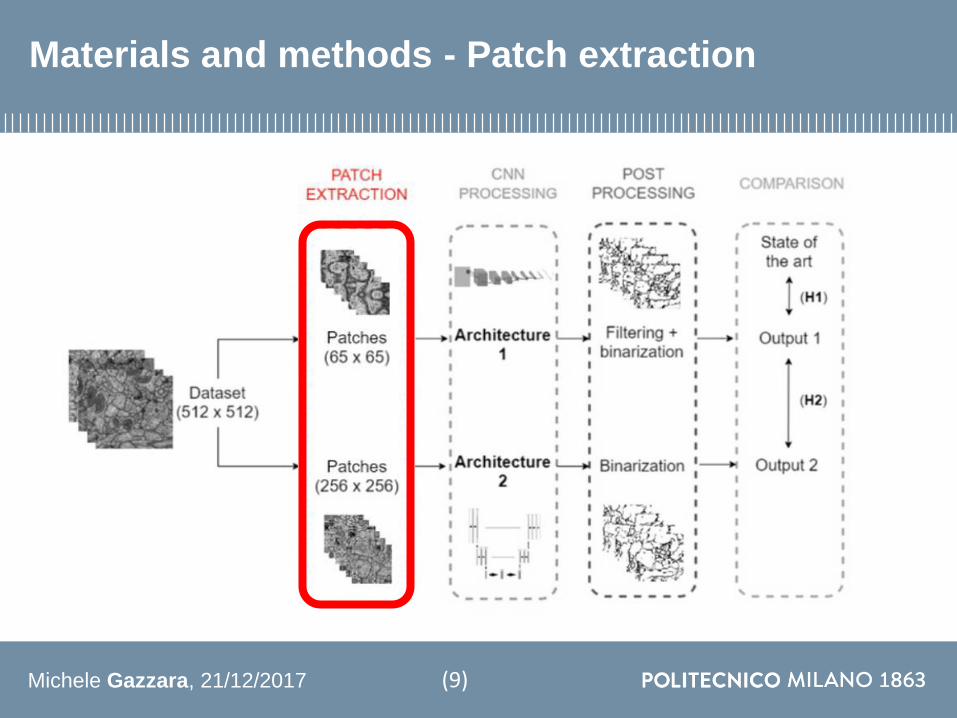
Michele Gazzara 21122017
Patch extraction
DATASET ISBI2012 Challenge dataset was used for the network training (20 images) andtesting (10 images) 30 512 x 512 sections from a serial section Transmission Electron Microscopy (ssTEM)
data set of the Drosophila first instar larva ventral nerve cord The microcube measures 2 x 2 x 15 microns with a resolution of 4x4x50 nmpixel
327˙680patches
(10)
Architecture 1(65 x 65 patches)
Michele Gazzara 21122017
Patch extraction
1920patches
(10)
DATASET ISBI2012 Challenge dataset was used for the network training (20 images) andtesting (10 images) 30 512 x 512 sections from a serial section Transmission Electron Microscopy (ssTEM)
data set of the Drosophila first instar larva ventral nerve cord The microcube measures 2 x 2 x 15 microns with a resolution of 4x4x50 nmpixel
Architecture 2(256 x 256 patches)
Michele Gazzara 21122017
Materials and methods - CNN processing
(11)
Michele Gazzara 21122017
Architecture 1
Input patch65 x 65
Output pixel probability
(12)
Michele Gazzara 21122017
Architecture 1
CL-10 CL-3CL-3CL-5
Input patch65 x 65
Output pixel probability
CL-n nxn conv
(12)
Michele Gazzara 21122017 (13)
Convolutional layer
Michele Gazzara 21122017
Architecture 1
CL-10 CL-3CL-3CL-5
Input patch65 x 65
Output pixel probability
CL-n nxn conv
ReLUReLU ReLU
Michele Gazzara 21122017 (14)
Rectifying Linear Unit (ReLU)
ReLU (119909) = ቊ0 119894119891 119909 le 0119909 119894119891 119909 gt 0
Michele Gazzara 21122017
Architecture 1
CL-10 CL-3CL-3MPCL-5MP MP
Input patch65 x 65
Output pixel probability
CL-n nxn conv MP 2x2 max pool
ReLUReLU ReLU
Michele Gazzara 21122017 (15)
Max pooling layer
Michele Gazzara 21122017
Architecture 1
CL-10 CL-3CL-3MPCL-5MP MP FCFC SM
Input patch65 x 65
Output pixel probability
CL-n nxn conv MP 2x2 max pool FC Fully connected layer SM Softmax layer
ReLUReLU ReLU
Michele Gazzara 21122017 (16)
Fully connected and Softmax layers
As many FC output valuesas the number of classes
p119895 = 119890119911119895
σ119898=1119872 119890119911119898
j = 0 1 hellip M
Where119963119947 is the FC output
M is the number of classes
Michele Gazzara 21122017
Architecture 1
CL-10 CL-3CL-3MPCL-5MP MP FCFC SM
Input patch65 x 65
Output pixel probability
CL-n nxn conv MP 2x2 max pool FC Fully connected layer SM Softmax layer
ReLUReLU ReLU
Michele Gazzara 21122017
Architecture 2
Output patch probability map
216 x 216
Input patch
256 x 256
(17)
Michele Gazzara 21122017
Architecture 2
Output patch probability map
216 x 216
Input patch
256 x 256
(17)
Michele Gazzara 21122017 (18)
Up-convolution
1) Up-sampling
2) 2x2 convolution
[O Ronneberger et al 2015]
Michele Gazzara 21122017
Architecture 2
Output patch probability map
216 x 216
Input patch
256 x 256
Michele Gazzara 21122017
Training settings
Cross EntropyWhereN number of samplesi sample indexy sample labelp sample probability
J = minus1
119873σ119894=1119873 119910119894 119897119900119892 119901119894 + 1 minus 119910119894 ∙ 119897119900119892(1 minus 119901119894)
(19)
[D Kline et al 2005]
Michele Gazzara 21122017
Training settings
Cross EntropyWhereN number of samplesi sample indexy sample labelp sample probability
J = minus1
119873σ119894=1119873 119910119894 119897119900119892 119901119894 + 1 minus 119910119894 ∙ 119897119900119892(1 minus 119901119894)
Mini-batch gradient descent
θ = θ minus 120578 120571120579 119869 (120579 119909(119894119894+119899) 119901(119894119894+119899))
Where120520 learning raten batch sizex input sample
(19)
[D Kline et al 2005]
[M Li et al 2014]
Michele Gazzara 21122017
Training settings
Cross EntropyWhereN number of samplesi sample indexy sample labelp sample probability
J = minus1
119873σ119894=1119873 119910119894 119897119900119892 119901119894 + 1 minus 119910119894 ∙ 119897119900119892(1 minus 119901119894)
Mini-batch gradient descent
Adam Optimizer
θ = θ minus 120578 120571120579 119869 (120579 119909(119894119894+119899) 119901(119894119894+119899))
Where120520 learning raten batch sizex input sample
θ119905+1119896 = θ119905119896 minus120578
119907119905 119892119905119896 + 120598
∙ 119898119905(119892119905119896)
Wheret batch indexk node indexv uncentered variancem meang gradient of J
(19)
[D Kingma et al 2014]
[D Kline et al 2005]
[M Li et al 2014]
Michele Gazzara 21122017
Materials and methods - Post processing
(20)
Michele Gazzara 21122017
Post processing
Architecture 1
Pixel probability
Spatial imagereconstruction
Medianfiltering
Otsuthresholding
(21)
Michele Gazzara 21122017
Post processing
Architecture 1
Pixel probability
Spatial imagereconstruction
Medianfiltering
Otsuthresholding
(21)
Patch probability
map
Otsuthresholding
Architecture 2
Michele Gazzara 21122017
Materials and methods - Comparison
(22)
Michele Gazzara 21122017
Evaluation protocol - Metrics
Accuracy (Acc)
Pixel error (PE)
Sensitivity (Sn) and Specificity (Sp)
SoslashrensenndashDice coefficient (DSC)
Sn = TP
TP+FN
PE = 1 - Acc
119860119888119888 =1
Nσj=1N 119904119888119900119903119890119895 score = ൝
1 119894119891 yj= ොy1198950 119894119891 yj ne ොy119895
119863119878119862 =2 119879119875
119865119875 + 119865119873 + 2 119879119875
Sp = TN
TN+FP
Where
119962119946 sample label
ෝ119962119946 prediction
N number of samples
i semple index
TP true positives
FN false negatives
TN true negatives
FP false positives
(23)
[I Arganda-Carreras et al 2015]
Michele Gazzara 21122017
Evaluation protocol - H1 and H2
Investigation of H1
VSNon CNN-based approaches
CNN-based approaches
Architecture 1(PE)
(24)
Investigation of H2
Architecture 1(Performance metrics and
computational costs)
Architecture 2(Performance metrics and
computational costs)
VS(Lilliefors and Wilcoxon test)
Michele Gazzara 21122017
Results - Investigation of H1
Model Method PE [∙10minus3]
Architecture 1 CNN 88
Kaynig et al (2010) RF 157
Liu et al (2012) ANN 134
Model Training images Training time PE [∙10minus3]
Architecture 1 327680 5 hours 10 min 88
Ciresan et al (2012) 3 millions 85 hours 60
Fakhry et al (2015) 42 millions 30 hours 51
Comparison with non-CNN based models
Comparison with other CNN based models
(25)
PE = 1 - Acc
Michele Gazzara 21122017
Evaluation protocol - H1 and H2
Investigation of H1
VSNon CNN-based approaches
CNN-based approaches
Architecture 1(PE)
Investigation of H2
Architecture 1(Performance metrics and
computational costs)
Architecture 2(Performance metrics and
computational costs)
VS(Lilliefors and Wilcoxon test)
Michele Gazzara 21122017
Results - Investigation of H2 metrics
(26)
Michele Gazzara 21122017
Results - Investigation of H2 computational costs
(27)
Michele Gazzara 21122017
Results - Segmented images
Architecture 2 output
Architecture 1 output
Input image Ground truth
(28)
Michele Gazzara 21122017
Discussion
H1
1 Architecture 1 performances exceed the non CNN-based models
2 Architecture 1 performances are comparable with other CNN-based models
Reduced dataset and training time
(29)
Michele Gazzara 21122017
Discussion
H1
1 Architecture 1 performances exceed the non CNN-based models
2 Architecture 1 performances are comparable with other CNN-based models
Reduced dataset and training time
H2
1 Architecture 2 overcomes Architecture 1in terms of accuracy
2 Architecture 2 computational costs are lower than Architecture 1
Architecture 1detects more FPs
Architecture 2 can be used for real
time applications
(29)
Michele Gazzara 21122017
Conclusions and future work
CONCLUSIONS
Automatic method for axon segmentation in EM images
Performances comparable with existing CNN models
Reduced computational costs
(30)
Michele Gazzara 21122017
Conclusions and future work
CONCLUSIONS
Automatic method for axon segmentation in EM images
Performances comparable with existing CNN models
Reduced computational costs
FUTURE WORK
Larger dataset
Human brain EM images
Up-convolution improvement
(30)
[H Gao et al 2017]
Michele Gazzara 21122017
Acknowledgements
(31)
Michele Gazzara 21122017
Thank you for your attention
(32)
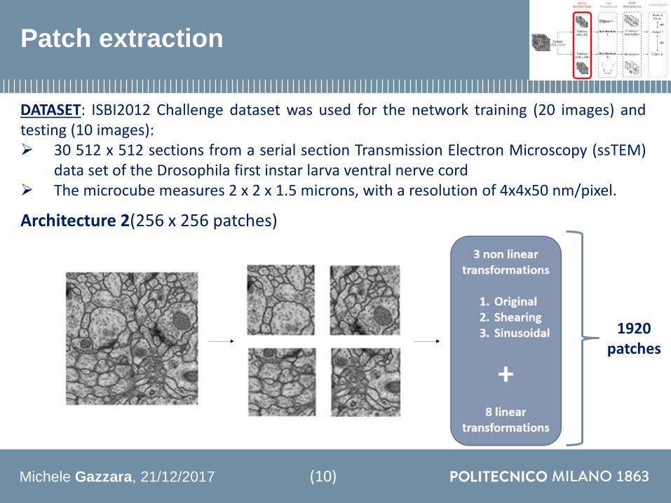
Michele Gazzara 21122017
Patch extraction
1920patches
(10)
DATASET ISBI2012 Challenge dataset was used for the network training (20 images) andtesting (10 images) 30 512 x 512 sections from a serial section Transmission Electron Microscopy (ssTEM)
data set of the Drosophila first instar larva ventral nerve cord The microcube measures 2 x 2 x 15 microns with a resolution of 4x4x50 nmpixel
Architecture 2(256 x 256 patches)
Michele Gazzara 21122017
Materials and methods - CNN processing
(11)
Michele Gazzara 21122017
Architecture 1
Input patch65 x 65
Output pixel probability
(12)
Michele Gazzara 21122017
Architecture 1
CL-10 CL-3CL-3CL-5
Input patch65 x 65
Output pixel probability
CL-n nxn conv
(12)
Michele Gazzara 21122017 (13)
Convolutional layer
Michele Gazzara 21122017
Architecture 1
CL-10 CL-3CL-3CL-5
Input patch65 x 65
Output pixel probability
CL-n nxn conv
ReLUReLU ReLU
Michele Gazzara 21122017 (14)
Rectifying Linear Unit (ReLU)
ReLU (119909) = ቊ0 119894119891 119909 le 0119909 119894119891 119909 gt 0
Michele Gazzara 21122017
Architecture 1
CL-10 CL-3CL-3MPCL-5MP MP
Input patch65 x 65
Output pixel probability
CL-n nxn conv MP 2x2 max pool
ReLUReLU ReLU
Michele Gazzara 21122017 (15)
Max pooling layer
Michele Gazzara 21122017
Architecture 1
CL-10 CL-3CL-3MPCL-5MP MP FCFC SM
Input patch65 x 65
Output pixel probability
CL-n nxn conv MP 2x2 max pool FC Fully connected layer SM Softmax layer
ReLUReLU ReLU
Michele Gazzara 21122017 (16)
Fully connected and Softmax layers
As many FC output valuesas the number of classes
p119895 = 119890119911119895
σ119898=1119872 119890119911119898
j = 0 1 hellip M
Where119963119947 is the FC output
M is the number of classes
Michele Gazzara 21122017
Architecture 1
CL-10 CL-3CL-3MPCL-5MP MP FCFC SM
Input patch65 x 65
Output pixel probability
CL-n nxn conv MP 2x2 max pool FC Fully connected layer SM Softmax layer
ReLUReLU ReLU
Michele Gazzara 21122017
Architecture 2
Output patch probability map
216 x 216
Input patch
256 x 256
(17)
Michele Gazzara 21122017
Architecture 2
Output patch probability map
216 x 216
Input patch
256 x 256
(17)
Michele Gazzara 21122017 (18)
Up-convolution
1) Up-sampling
2) 2x2 convolution
[O Ronneberger et al 2015]
Michele Gazzara 21122017
Architecture 2
Output patch probability map
216 x 216
Input patch
256 x 256
Michele Gazzara 21122017
Training settings
Cross EntropyWhereN number of samplesi sample indexy sample labelp sample probability
J = minus1
119873σ119894=1119873 119910119894 119897119900119892 119901119894 + 1 minus 119910119894 ∙ 119897119900119892(1 minus 119901119894)
(19)
[D Kline et al 2005]
Michele Gazzara 21122017
Training settings
Cross EntropyWhereN number of samplesi sample indexy sample labelp sample probability
J = minus1
119873σ119894=1119873 119910119894 119897119900119892 119901119894 + 1 minus 119910119894 ∙ 119897119900119892(1 minus 119901119894)
Mini-batch gradient descent
θ = θ minus 120578 120571120579 119869 (120579 119909(119894119894+119899) 119901(119894119894+119899))
Where120520 learning raten batch sizex input sample
(19)
[D Kline et al 2005]
[M Li et al 2014]
Michele Gazzara 21122017
Training settings
Cross EntropyWhereN number of samplesi sample indexy sample labelp sample probability
J = minus1
119873σ119894=1119873 119910119894 119897119900119892 119901119894 + 1 minus 119910119894 ∙ 119897119900119892(1 minus 119901119894)
Mini-batch gradient descent
Adam Optimizer
θ = θ minus 120578 120571120579 119869 (120579 119909(119894119894+119899) 119901(119894119894+119899))
Where120520 learning raten batch sizex input sample
θ119905+1119896 = θ119905119896 minus120578
119907119905 119892119905119896 + 120598
∙ 119898119905(119892119905119896)
Wheret batch indexk node indexv uncentered variancem meang gradient of J
(19)
[D Kingma et al 2014]
[D Kline et al 2005]
[M Li et al 2014]
Michele Gazzara 21122017
Materials and methods - Post processing
(20)
Michele Gazzara 21122017
Post processing
Architecture 1
Pixel probability
Spatial imagereconstruction
Medianfiltering
Otsuthresholding
(21)
Michele Gazzara 21122017
Post processing
Architecture 1
Pixel probability
Spatial imagereconstruction
Medianfiltering
Otsuthresholding
(21)
Patch probability
map
Otsuthresholding
Architecture 2
Michele Gazzara 21122017
Materials and methods - Comparison
(22)
Michele Gazzara 21122017
Evaluation protocol - Metrics
Accuracy (Acc)
Pixel error (PE)
Sensitivity (Sn) and Specificity (Sp)
SoslashrensenndashDice coefficient (DSC)
Sn = TP
TP+FN
PE = 1 - Acc
119860119888119888 =1
Nσj=1N 119904119888119900119903119890119895 score = ൝
1 119894119891 yj= ොy1198950 119894119891 yj ne ොy119895
119863119878119862 =2 119879119875
119865119875 + 119865119873 + 2 119879119875
Sp = TN
TN+FP
Where
119962119946 sample label
ෝ119962119946 prediction
N number of samples
i semple index
TP true positives
FN false negatives
TN true negatives
FP false positives
(23)
[I Arganda-Carreras et al 2015]
Michele Gazzara 21122017
Evaluation protocol - H1 and H2
Investigation of H1
VSNon CNN-based approaches
CNN-based approaches
Architecture 1(PE)
(24)
Investigation of H2
Architecture 1(Performance metrics and
computational costs)
Architecture 2(Performance metrics and
computational costs)
VS(Lilliefors and Wilcoxon test)
Michele Gazzara 21122017
Results - Investigation of H1
Model Method PE [∙10minus3]
Architecture 1 CNN 88
Kaynig et al (2010) RF 157
Liu et al (2012) ANN 134
Model Training images Training time PE [∙10minus3]
Architecture 1 327680 5 hours 10 min 88
Ciresan et al (2012) 3 millions 85 hours 60
Fakhry et al (2015) 42 millions 30 hours 51
Comparison with non-CNN based models
Comparison with other CNN based models
(25)
PE = 1 - Acc
Michele Gazzara 21122017
Evaluation protocol - H1 and H2
Investigation of H1
VSNon CNN-based approaches
CNN-based approaches
Architecture 1(PE)
Investigation of H2
Architecture 1(Performance metrics and
computational costs)
Architecture 2(Performance metrics and
computational costs)
VS(Lilliefors and Wilcoxon test)
Michele Gazzara 21122017
Results - Investigation of H2 metrics
(26)
Michele Gazzara 21122017
Results - Investigation of H2 computational costs
(27)
Michele Gazzara 21122017
Results - Segmented images
Architecture 2 output
Architecture 1 output
Input image Ground truth
(28)
Michele Gazzara 21122017
Discussion
H1
1 Architecture 1 performances exceed the non CNN-based models
2 Architecture 1 performances are comparable with other CNN-based models
Reduced dataset and training time
(29)
Michele Gazzara 21122017
Discussion
H1
1 Architecture 1 performances exceed the non CNN-based models
2 Architecture 1 performances are comparable with other CNN-based models
Reduced dataset and training time
H2
1 Architecture 2 overcomes Architecture 1in terms of accuracy
2 Architecture 2 computational costs are lower than Architecture 1
Architecture 1detects more FPs
Architecture 2 can be used for real
time applications
(29)
Michele Gazzara 21122017
Conclusions and future work
CONCLUSIONS
Automatic method for axon segmentation in EM images
Performances comparable with existing CNN models
Reduced computational costs
(30)
Michele Gazzara 21122017
Conclusions and future work
CONCLUSIONS
Automatic method for axon segmentation in EM images
Performances comparable with existing CNN models
Reduced computational costs
FUTURE WORK
Larger dataset
Human brain EM images
Up-convolution improvement
(30)
[H Gao et al 2017]
Michele Gazzara 21122017
Acknowledgements
(31)
Michele Gazzara 21122017
Thank you for your attention
(32)
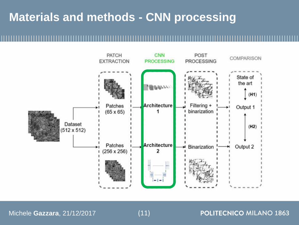
Michele Gazzara 21122017
Architecture 1
Input patch65 x 65
Output pixel probability
(12)
Michele Gazzara 21122017
Architecture 1
CL-10 CL-3CL-3CL-5
Input patch65 x 65
Output pixel probability
CL-n nxn conv
(12)
Michele Gazzara 21122017 (13)
Convolutional layer
Michele Gazzara 21122017
Architecture 1
CL-10 CL-3CL-3CL-5
Input patch65 x 65
Output pixel probability
CL-n nxn conv
ReLUReLU ReLU
Michele Gazzara 21122017 (14)
Rectifying Linear Unit (ReLU)
ReLU (119909) = ቊ0 119894119891 119909 le 0119909 119894119891 119909 gt 0
Michele Gazzara 21122017
Architecture 1
CL-10 CL-3CL-3MPCL-5MP MP
Input patch65 x 65
Output pixel probability
CL-n nxn conv MP 2x2 max pool
ReLUReLU ReLU
Michele Gazzara 21122017 (15)
Max pooling layer
Michele Gazzara 21122017
Architecture 1
CL-10 CL-3CL-3MPCL-5MP MP FCFC SM
Input patch65 x 65
Output pixel probability
CL-n nxn conv MP 2x2 max pool FC Fully connected layer SM Softmax layer
ReLUReLU ReLU
Michele Gazzara 21122017 (16)
Fully connected and Softmax layers
As many FC output valuesas the number of classes
p119895 = 119890119911119895
σ119898=1119872 119890119911119898
j = 0 1 hellip M
Where119963119947 is the FC output
M is the number of classes
Michele Gazzara 21122017
Architecture 1
CL-10 CL-3CL-3MPCL-5MP MP FCFC SM
Input patch65 x 65
Output pixel probability
CL-n nxn conv MP 2x2 max pool FC Fully connected layer SM Softmax layer
ReLUReLU ReLU
Michele Gazzara 21122017
Architecture 2
Output patch probability map
216 x 216
Input patch
256 x 256
(17)
Michele Gazzara 21122017
Architecture 2
Output patch probability map
216 x 216
Input patch
256 x 256
(17)
Michele Gazzara 21122017 (18)
Up-convolution
1) Up-sampling
2) 2x2 convolution
[O Ronneberger et al 2015]
Michele Gazzara 21122017
Architecture 2
Output patch probability map
216 x 216
Input patch
256 x 256
Michele Gazzara 21122017
Training settings
Cross EntropyWhereN number of samplesi sample indexy sample labelp sample probability
J = minus1
119873σ119894=1119873 119910119894 119897119900119892 119901119894 + 1 minus 119910119894 ∙ 119897119900119892(1 minus 119901119894)
(19)
[D Kline et al 2005]
Michele Gazzara 21122017
Training settings
Cross EntropyWhereN number of samplesi sample indexy sample labelp sample probability
J = minus1
119873σ119894=1119873 119910119894 119897119900119892 119901119894 + 1 minus 119910119894 ∙ 119897119900119892(1 minus 119901119894)
Mini-batch gradient descent
θ = θ minus 120578 120571120579 119869 (120579 119909(119894119894+119899) 119901(119894119894+119899))
Where120520 learning raten batch sizex input sample
(19)
[D Kline et al 2005]
[M Li et al 2014]
Michele Gazzara 21122017
Training settings
Cross EntropyWhereN number of samplesi sample indexy sample labelp sample probability
J = minus1
119873σ119894=1119873 119910119894 119897119900119892 119901119894 + 1 minus 119910119894 ∙ 119897119900119892(1 minus 119901119894)
Mini-batch gradient descent
Adam Optimizer
θ = θ minus 120578 120571120579 119869 (120579 119909(119894119894+119899) 119901(119894119894+119899))
Where120520 learning raten batch sizex input sample
θ119905+1119896 = θ119905119896 minus120578
119907119905 119892119905119896 + 120598
∙ 119898119905(119892119905119896)
Wheret batch indexk node indexv uncentered variancem meang gradient of J
(19)
[D Kingma et al 2014]
[D Kline et al 2005]
[M Li et al 2014]
Michele Gazzara 21122017
Materials and methods - Post processing
(20)
Michele Gazzara 21122017
Post processing
Architecture 1
Pixel probability
Spatial imagereconstruction
Medianfiltering
Otsuthresholding
(21)
Michele Gazzara 21122017
Post processing
Architecture 1
Pixel probability
Spatial imagereconstruction
Medianfiltering
Otsuthresholding
(21)
Patch probability
map
Otsuthresholding
Architecture 2
Michele Gazzara 21122017
Materials and methods - Comparison
(22)
Michele Gazzara 21122017
Evaluation protocol - Metrics
Accuracy (Acc)
Pixel error (PE)
Sensitivity (Sn) and Specificity (Sp)
SoslashrensenndashDice coefficient (DSC)
Sn = TP
TP+FN
PE = 1 - Acc
119860119888119888 =1
Nσj=1N 119904119888119900119903119890119895 score = ൝
1 119894119891 yj= ොy1198950 119894119891 yj ne ොy119895
119863119878119862 =2 119879119875
119865119875 + 119865119873 + 2 119879119875
Sp = TN
TN+FP
Where
119962119946 sample label
ෝ119962119946 prediction
N number of samples
i semple index
TP true positives
FN false negatives
TN true negatives
FP false positives
(23)
[I Arganda-Carreras et al 2015]
Michele Gazzara 21122017
Evaluation protocol - H1 and H2
Investigation of H1
VSNon CNN-based approaches
CNN-based approaches
Architecture 1(PE)
(24)
Investigation of H2
Architecture 1(Performance metrics and
computational costs)
Architecture 2(Performance metrics and
computational costs)
VS(Lilliefors and Wilcoxon test)
Michele Gazzara 21122017
Results - Investigation of H1
Model Method PE [∙10minus3]
Architecture 1 CNN 88
Kaynig et al (2010) RF 157
Liu et al (2012) ANN 134
Model Training images Training time PE [∙10minus3]
Architecture 1 327680 5 hours 10 min 88
Ciresan et al (2012) 3 millions 85 hours 60
Fakhry et al (2015) 42 millions 30 hours 51
Comparison with non-CNN based models
Comparison with other CNN based models
(25)
PE = 1 - Acc
Michele Gazzara 21122017
Evaluation protocol - H1 and H2
Investigation of H1
VSNon CNN-based approaches
CNN-based approaches
Architecture 1(PE)
Investigation of H2
Architecture 1(Performance metrics and
computational costs)
Architecture 2(Performance metrics and
computational costs)
VS(Lilliefors and Wilcoxon test)
Michele Gazzara 21122017
Results - Investigation of H2 metrics
(26)
Michele Gazzara 21122017
Results - Investigation of H2 computational costs
(27)
Michele Gazzara 21122017
Results - Segmented images
Architecture 2 output
Architecture 1 output
Input image Ground truth
(28)
Michele Gazzara 21122017
Discussion
H1
1 Architecture 1 performances exceed the non CNN-based models
2 Architecture 1 performances are comparable with other CNN-based models
Reduced dataset and training time
(29)
Michele Gazzara 21122017
Discussion
H1
1 Architecture 1 performances exceed the non CNN-based models
2 Architecture 1 performances are comparable with other CNN-based models
Reduced dataset and training time
H2
1 Architecture 2 overcomes Architecture 1in terms of accuracy
2 Architecture 2 computational costs are lower than Architecture 1
Architecture 1detects more FPs
Architecture 2 can be used for real
time applications
(29)
Michele Gazzara 21122017
Conclusions and future work
CONCLUSIONS
Automatic method for axon segmentation in EM images
Performances comparable with existing CNN models
Reduced computational costs
(30)
Michele Gazzara 21122017
Conclusions and future work
CONCLUSIONS
Automatic method for axon segmentation in EM images
Performances comparable with existing CNN models
Reduced computational costs
FUTURE WORK
Larger dataset
Human brain EM images
Up-convolution improvement
(30)
[H Gao et al 2017]
Michele Gazzara 21122017
Acknowledgements
(31)
Michele Gazzara 21122017
Thank you for your attention
(32)

Michele Gazzara 21122017
Architecture 1
CL-10 CL-3CL-3CL-5
Input patch65 x 65
Output pixel probability
CL-n nxn conv
(12)
Michele Gazzara 21122017 (13)
Convolutional layer
Michele Gazzara 21122017
Architecture 1
CL-10 CL-3CL-3CL-5
Input patch65 x 65
Output pixel probability
CL-n nxn conv
ReLUReLU ReLU
Michele Gazzara 21122017 (14)
Rectifying Linear Unit (ReLU)
ReLU (119909) = ቊ0 119894119891 119909 le 0119909 119894119891 119909 gt 0
Michele Gazzara 21122017
Architecture 1
CL-10 CL-3CL-3MPCL-5MP MP
Input patch65 x 65
Output pixel probability
CL-n nxn conv MP 2x2 max pool
ReLUReLU ReLU
Michele Gazzara 21122017 (15)
Max pooling layer
Michele Gazzara 21122017
Architecture 1
CL-10 CL-3CL-3MPCL-5MP MP FCFC SM
Input patch65 x 65
Output pixel probability
CL-n nxn conv MP 2x2 max pool FC Fully connected layer SM Softmax layer
ReLUReLU ReLU
Michele Gazzara 21122017 (16)
Fully connected and Softmax layers
As many FC output valuesas the number of classes
p119895 = 119890119911119895
σ119898=1119872 119890119911119898
j = 0 1 hellip M
Where119963119947 is the FC output
M is the number of classes
Michele Gazzara 21122017
Architecture 1
CL-10 CL-3CL-3MPCL-5MP MP FCFC SM
Input patch65 x 65
Output pixel probability
CL-n nxn conv MP 2x2 max pool FC Fully connected layer SM Softmax layer
ReLUReLU ReLU
Michele Gazzara 21122017
Architecture 2
Output patch probability map
216 x 216
Input patch
256 x 256
(17)
Michele Gazzara 21122017
Architecture 2
Output patch probability map
216 x 216
Input patch
256 x 256
(17)
Michele Gazzara 21122017 (18)
Up-convolution
1) Up-sampling
2) 2x2 convolution
[O Ronneberger et al 2015]
Michele Gazzara 21122017
Architecture 2
Output patch probability map
216 x 216
Input patch
256 x 256
Michele Gazzara 21122017
Training settings
Cross EntropyWhereN number of samplesi sample indexy sample labelp sample probability
J = minus1
119873σ119894=1119873 119910119894 119897119900119892 119901119894 + 1 minus 119910119894 ∙ 119897119900119892(1 minus 119901119894)
(19)
[D Kline et al 2005]
Michele Gazzara 21122017
Training settings
Cross EntropyWhereN number of samplesi sample indexy sample labelp sample probability
J = minus1
119873σ119894=1119873 119910119894 119897119900119892 119901119894 + 1 minus 119910119894 ∙ 119897119900119892(1 minus 119901119894)
Mini-batch gradient descent
θ = θ minus 120578 120571120579 119869 (120579 119909(119894119894+119899) 119901(119894119894+119899))
Where120520 learning raten batch sizex input sample
(19)
[D Kline et al 2005]
[M Li et al 2014]
Michele Gazzara 21122017
Training settings
Cross EntropyWhereN number of samplesi sample indexy sample labelp sample probability
J = minus1
119873σ119894=1119873 119910119894 119897119900119892 119901119894 + 1 minus 119910119894 ∙ 119897119900119892(1 minus 119901119894)
Mini-batch gradient descent
Adam Optimizer
θ = θ minus 120578 120571120579 119869 (120579 119909(119894119894+119899) 119901(119894119894+119899))
Where120520 learning raten batch sizex input sample
θ119905+1119896 = θ119905119896 minus120578
119907119905 119892119905119896 + 120598
∙ 119898119905(119892119905119896)
Wheret batch indexk node indexv uncentered variancem meang gradient of J
(19)
[D Kingma et al 2014]
[D Kline et al 2005]
[M Li et al 2014]
Michele Gazzara 21122017
Materials and methods - Post processing
(20)
Michele Gazzara 21122017
Post processing
Architecture 1
Pixel probability
Spatial imagereconstruction
Medianfiltering
Otsuthresholding
(21)
Michele Gazzara 21122017
Post processing
Architecture 1
Pixel probability
Spatial imagereconstruction
Medianfiltering
Otsuthresholding
(21)
Patch probability
map
Otsuthresholding
Architecture 2
Michele Gazzara 21122017
Materials and methods - Comparison
(22)
Michele Gazzara 21122017
Evaluation protocol - Metrics
Accuracy (Acc)
Pixel error (PE)
Sensitivity (Sn) and Specificity (Sp)
SoslashrensenndashDice coefficient (DSC)
Sn = TP
TP+FN
PE = 1 - Acc
119860119888119888 =1
Nσj=1N 119904119888119900119903119890119895 score = ൝
1 119894119891 yj= ොy1198950 119894119891 yj ne ොy119895
119863119878119862 =2 119879119875
119865119875 + 119865119873 + 2 119879119875
Sp = TN
TN+FP
Where
119962119946 sample label
ෝ119962119946 prediction
N number of samples
i semple index
TP true positives
FN false negatives
TN true negatives
FP false positives
(23)
[I Arganda-Carreras et al 2015]
Michele Gazzara 21122017
Evaluation protocol - H1 and H2
Investigation of H1
VSNon CNN-based approaches
CNN-based approaches
Architecture 1(PE)
(24)
Investigation of H2
Architecture 1(Performance metrics and
computational costs)
Architecture 2(Performance metrics and
computational costs)
VS(Lilliefors and Wilcoxon test)
Michele Gazzara 21122017
Results - Investigation of H1
Model Method PE [∙10minus3]
Architecture 1 CNN 88
Kaynig et al (2010) RF 157
Liu et al (2012) ANN 134
Model Training images Training time PE [∙10minus3]
Architecture 1 327680 5 hours 10 min 88
Ciresan et al (2012) 3 millions 85 hours 60
Fakhry et al (2015) 42 millions 30 hours 51
Comparison with non-CNN based models
Comparison with other CNN based models
(25)
PE = 1 - Acc
Michele Gazzara 21122017
Evaluation protocol - H1 and H2
Investigation of H1
VSNon CNN-based approaches
CNN-based approaches
Architecture 1(PE)
Investigation of H2
Architecture 1(Performance metrics and
computational costs)
Architecture 2(Performance metrics and
computational costs)
VS(Lilliefors and Wilcoxon test)
Michele Gazzara 21122017
Results - Investigation of H2 metrics
(26)
Michele Gazzara 21122017
Results - Investigation of H2 computational costs
(27)
Michele Gazzara 21122017
Results - Segmented images
Architecture 2 output
Architecture 1 output
Input image Ground truth
(28)
Michele Gazzara 21122017
Discussion
H1
1 Architecture 1 performances exceed the non CNN-based models
2 Architecture 1 performances are comparable with other CNN-based models
Reduced dataset and training time
(29)
Michele Gazzara 21122017
Discussion
H1
1 Architecture 1 performances exceed the non CNN-based models
2 Architecture 1 performances are comparable with other CNN-based models
Reduced dataset and training time
H2
1 Architecture 2 overcomes Architecture 1in terms of accuracy
2 Architecture 2 computational costs are lower than Architecture 1
Architecture 1detects more FPs
Architecture 2 can be used for real
time applications
(29)
Michele Gazzara 21122017
Conclusions and future work
CONCLUSIONS
Automatic method for axon segmentation in EM images
Performances comparable with existing CNN models
Reduced computational costs
(30)
Michele Gazzara 21122017
Conclusions and future work
CONCLUSIONS
Automatic method for axon segmentation in EM images
Performances comparable with existing CNN models
Reduced computational costs
FUTURE WORK
Larger dataset
Human brain EM images
Up-convolution improvement
(30)
[H Gao et al 2017]
Michele Gazzara 21122017
Acknowledgements
(31)
Michele Gazzara 21122017
Thank you for your attention
(32)
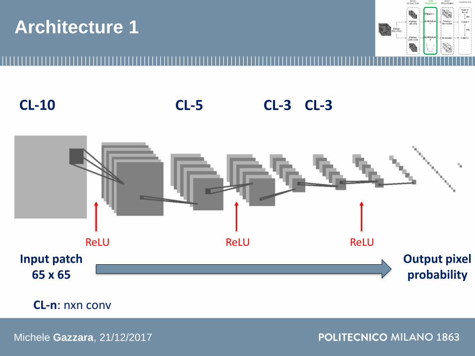
Michele Gazzara 21122017
Architecture 1
CL-10 CL-3CL-3CL-5
Input patch65 x 65
Output pixel probability
CL-n nxn conv
ReLUReLU ReLU
Michele Gazzara 21122017 (14)
Rectifying Linear Unit (ReLU)
ReLU (119909) = ቊ0 119894119891 119909 le 0119909 119894119891 119909 gt 0
Michele Gazzara 21122017
Architecture 1
CL-10 CL-3CL-3MPCL-5MP MP
Input patch65 x 65
Output pixel probability
CL-n nxn conv MP 2x2 max pool
ReLUReLU ReLU
Michele Gazzara 21122017 (15)
Max pooling layer
Michele Gazzara 21122017
Architecture 1
CL-10 CL-3CL-3MPCL-5MP MP FCFC SM
Input patch65 x 65
Output pixel probability
CL-n nxn conv MP 2x2 max pool FC Fully connected layer SM Softmax layer
ReLUReLU ReLU
Michele Gazzara 21122017 (16)
Fully connected and Softmax layers
As many FC output valuesas the number of classes
p119895 = 119890119911119895
σ119898=1119872 119890119911119898
j = 0 1 hellip M
Where119963119947 is the FC output
M is the number of classes
Michele Gazzara 21122017
Architecture 1
CL-10 CL-3CL-3MPCL-5MP MP FCFC SM
Input patch65 x 65
Output pixel probability
CL-n nxn conv MP 2x2 max pool FC Fully connected layer SM Softmax layer
ReLUReLU ReLU
Michele Gazzara 21122017
Architecture 2
Output patch probability map
216 x 216
Input patch
256 x 256
(17)
Michele Gazzara 21122017
Architecture 2
Output patch probability map
216 x 216
Input patch
256 x 256
(17)
Michele Gazzara 21122017 (18)
Up-convolution
1) Up-sampling
2) 2x2 convolution
[O Ronneberger et al 2015]
Michele Gazzara 21122017
Architecture 2
Output patch probability map
216 x 216
Input patch
256 x 256
Michele Gazzara 21122017
Training settings
Cross EntropyWhereN number of samplesi sample indexy sample labelp sample probability
J = minus1
119873σ119894=1119873 119910119894 119897119900119892 119901119894 + 1 minus 119910119894 ∙ 119897119900119892(1 minus 119901119894)
(19)
[D Kline et al 2005]
Michele Gazzara 21122017
Training settings
Cross EntropyWhereN number of samplesi sample indexy sample labelp sample probability
J = minus1
119873σ119894=1119873 119910119894 119897119900119892 119901119894 + 1 minus 119910119894 ∙ 119897119900119892(1 minus 119901119894)
Mini-batch gradient descent
θ = θ minus 120578 120571120579 119869 (120579 119909(119894119894+119899) 119901(119894119894+119899))
Where120520 learning raten batch sizex input sample
(19)
[D Kline et al 2005]
[M Li et al 2014]
Michele Gazzara 21122017
Training settings
Cross EntropyWhereN number of samplesi sample indexy sample labelp sample probability
J = minus1
119873σ119894=1119873 119910119894 119897119900119892 119901119894 + 1 minus 119910119894 ∙ 119897119900119892(1 minus 119901119894)
Mini-batch gradient descent
Adam Optimizer
θ = θ minus 120578 120571120579 119869 (120579 119909(119894119894+119899) 119901(119894119894+119899))
Where120520 learning raten batch sizex input sample
θ119905+1119896 = θ119905119896 minus120578
119907119905 119892119905119896 + 120598
∙ 119898119905(119892119905119896)
Wheret batch indexk node indexv uncentered variancem meang gradient of J
(19)
[D Kingma et al 2014]
[D Kline et al 2005]
[M Li et al 2014]
Michele Gazzara 21122017
Materials and methods - Post processing
(20)
Michele Gazzara 21122017
Post processing
Architecture 1
Pixel probability
Spatial imagereconstruction
Medianfiltering
Otsuthresholding
(21)
Michele Gazzara 21122017
Post processing
Architecture 1
Pixel probability
Spatial imagereconstruction
Medianfiltering
Otsuthresholding
(21)
Patch probability
map
Otsuthresholding
Architecture 2
Michele Gazzara 21122017
Materials and methods - Comparison
(22)
Michele Gazzara 21122017
Evaluation protocol - Metrics
Accuracy (Acc)
Pixel error (PE)
Sensitivity (Sn) and Specificity (Sp)
SoslashrensenndashDice coefficient (DSC)
Sn = TP
TP+FN
PE = 1 - Acc
119860119888119888 =1
Nσj=1N 119904119888119900119903119890119895 score = ൝
1 119894119891 yj= ොy1198950 119894119891 yj ne ොy119895
119863119878119862 =2 119879119875
119865119875 + 119865119873 + 2 119879119875
Sp = TN
TN+FP
Where
119962119946 sample label
ෝ119962119946 prediction
N number of samples
i semple index
TP true positives
FN false negatives
TN true negatives
FP false positives
(23)
[I Arganda-Carreras et al 2015]
Michele Gazzara 21122017
Evaluation protocol - H1 and H2
Investigation of H1
VSNon CNN-based approaches
CNN-based approaches
Architecture 1(PE)
(24)
Investigation of H2
Architecture 1(Performance metrics and
computational costs)
Architecture 2(Performance metrics and
computational costs)
VS(Lilliefors and Wilcoxon test)
Michele Gazzara 21122017
Results - Investigation of H1
Model Method PE [∙10minus3]
Architecture 1 CNN 88
Kaynig et al (2010) RF 157
Liu et al (2012) ANN 134
Model Training images Training time PE [∙10minus3]
Architecture 1 327680 5 hours 10 min 88
Ciresan et al (2012) 3 millions 85 hours 60
Fakhry et al (2015) 42 millions 30 hours 51
Comparison with non-CNN based models
Comparison with other CNN based models
(25)
PE = 1 - Acc
Michele Gazzara 21122017
Evaluation protocol - H1 and H2
Investigation of H1
VSNon CNN-based approaches
CNN-based approaches
Architecture 1(PE)
Investigation of H2
Architecture 1(Performance metrics and
computational costs)
Architecture 2(Performance metrics and
computational costs)
VS(Lilliefors and Wilcoxon test)
Michele Gazzara 21122017
Results - Investigation of H2 metrics
(26)
Michele Gazzara 21122017
Results - Investigation of H2 computational costs
(27)
Michele Gazzara 21122017
Results - Segmented images
Architecture 2 output
Architecture 1 output
Input image Ground truth
(28)
Michele Gazzara 21122017
Discussion
H1
1 Architecture 1 performances exceed the non CNN-based models
2 Architecture 1 performances are comparable with other CNN-based models
Reduced dataset and training time
(29)
Michele Gazzara 21122017
Discussion
H1
1 Architecture 1 performances exceed the non CNN-based models
2 Architecture 1 performances are comparable with other CNN-based models
Reduced dataset and training time
H2
1 Architecture 2 overcomes Architecture 1in terms of accuracy
2 Architecture 2 computational costs are lower than Architecture 1
Architecture 1detects more FPs
Architecture 2 can be used for real
time applications
(29)
Michele Gazzara 21122017
Conclusions and future work
CONCLUSIONS
Automatic method for axon segmentation in EM images
Performances comparable with existing CNN models
Reduced computational costs
(30)
Michele Gazzara 21122017
Conclusions and future work
CONCLUSIONS
Automatic method for axon segmentation in EM images
Performances comparable with existing CNN models
Reduced computational costs
FUTURE WORK
Larger dataset
Human brain EM images
Up-convolution improvement
(30)
[H Gao et al 2017]
Michele Gazzara 21122017
Acknowledgements
(31)
Michele Gazzara 21122017
Thank you for your attention
(32)
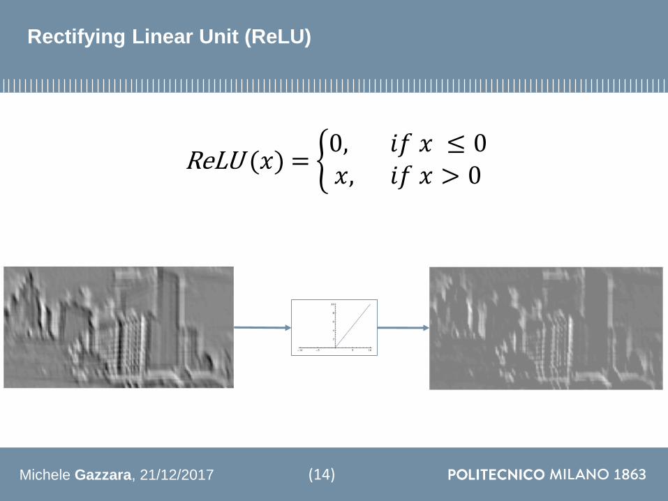

Michele Gazzara 21122017
Architecture 1
CL-10 CL-3CL-3MPCL-5MP MP
Input patch65 x 65
Output pixel probability
CL-n nxn conv MP 2x2 max pool
ReLUReLU ReLU
Michele Gazzara 21122017 (15)
Max pooling layer
Michele Gazzara 21122017
Architecture 1
CL-10 CL-3CL-3MPCL-5MP MP FCFC SM
Input patch65 x 65
Output pixel probability
CL-n nxn conv MP 2x2 max pool FC Fully connected layer SM Softmax layer
ReLUReLU ReLU
Michele Gazzara 21122017 (16)
Fully connected and Softmax layers
As many FC output valuesas the number of classes
p119895 = 119890119911119895
σ119898=1119872 119890119911119898
j = 0 1 hellip M
Where119963119947 is the FC output
M is the number of classes
Michele Gazzara 21122017
Architecture 1
CL-10 CL-3CL-3MPCL-5MP MP FCFC SM
Input patch65 x 65
Output pixel probability
CL-n nxn conv MP 2x2 max pool FC Fully connected layer SM Softmax layer
ReLUReLU ReLU
Michele Gazzara 21122017
Architecture 2
Output patch probability map
216 x 216
Input patch
256 x 256
(17)
Michele Gazzara 21122017
Architecture 2
Output patch probability map
216 x 216
Input patch
256 x 256
(17)
Michele Gazzara 21122017 (18)
Up-convolution
1) Up-sampling
2) 2x2 convolution
[O Ronneberger et al 2015]
Michele Gazzara 21122017
Architecture 2
Output patch probability map
216 x 216
Input patch
256 x 256
Michele Gazzara 21122017
Training settings
Cross EntropyWhereN number of samplesi sample indexy sample labelp sample probability
J = minus1
119873σ119894=1119873 119910119894 119897119900119892 119901119894 + 1 minus 119910119894 ∙ 119897119900119892(1 minus 119901119894)
(19)
[D Kline et al 2005]
Michele Gazzara 21122017
Training settings
Cross EntropyWhereN number of samplesi sample indexy sample labelp sample probability
J = minus1
119873σ119894=1119873 119910119894 119897119900119892 119901119894 + 1 minus 119910119894 ∙ 119897119900119892(1 minus 119901119894)
Mini-batch gradient descent
θ = θ minus 120578 120571120579 119869 (120579 119909(119894119894+119899) 119901(119894119894+119899))
Where120520 learning raten batch sizex input sample
(19)
[D Kline et al 2005]
[M Li et al 2014]
Michele Gazzara 21122017
Training settings
Cross EntropyWhereN number of samplesi sample indexy sample labelp sample probability
J = minus1
119873σ119894=1119873 119910119894 119897119900119892 119901119894 + 1 minus 119910119894 ∙ 119897119900119892(1 minus 119901119894)
Mini-batch gradient descent
Adam Optimizer
θ = θ minus 120578 120571120579 119869 (120579 119909(119894119894+119899) 119901(119894119894+119899))
Where120520 learning raten batch sizex input sample
θ119905+1119896 = θ119905119896 minus120578
119907119905 119892119905119896 + 120598
∙ 119898119905(119892119905119896)
Wheret batch indexk node indexv uncentered variancem meang gradient of J
(19)
[D Kingma et al 2014]
[D Kline et al 2005]
[M Li et al 2014]
Michele Gazzara 21122017
Materials and methods - Post processing
(20)
Michele Gazzara 21122017
Post processing
Architecture 1
Pixel probability
Spatial imagereconstruction
Medianfiltering
Otsuthresholding
(21)
Michele Gazzara 21122017
Post processing
Architecture 1
Pixel probability
Spatial imagereconstruction
Medianfiltering
Otsuthresholding
(21)
Patch probability
map
Otsuthresholding
Architecture 2
Michele Gazzara 21122017
Materials and methods - Comparison
(22)
Michele Gazzara 21122017
Evaluation protocol - Metrics
Accuracy (Acc)
Pixel error (PE)
Sensitivity (Sn) and Specificity (Sp)
SoslashrensenndashDice coefficient (DSC)
Sn = TP
TP+FN
PE = 1 - Acc
119860119888119888 =1
Nσj=1N 119904119888119900119903119890119895 score = ൝
1 119894119891 yj= ොy1198950 119894119891 yj ne ොy119895
119863119878119862 =2 119879119875
119865119875 + 119865119873 + 2 119879119875
Sp = TN
TN+FP
Where
119962119946 sample label
ෝ119962119946 prediction
N number of samples
i semple index
TP true positives
FN false negatives
TN true negatives
FP false positives
(23)
[I Arganda-Carreras et al 2015]
Michele Gazzara 21122017
Evaluation protocol - H1 and H2
Investigation of H1
VSNon CNN-based approaches
CNN-based approaches
Architecture 1(PE)
(24)
Investigation of H2
Architecture 1(Performance metrics and
computational costs)
Architecture 2(Performance metrics and
computational costs)
VS(Lilliefors and Wilcoxon test)
Michele Gazzara 21122017
Results - Investigation of H1
Model Method PE [∙10minus3]
Architecture 1 CNN 88
Kaynig et al (2010) RF 157
Liu et al (2012) ANN 134
Model Training images Training time PE [∙10minus3]
Architecture 1 327680 5 hours 10 min 88
Ciresan et al (2012) 3 millions 85 hours 60
Fakhry et al (2015) 42 millions 30 hours 51
Comparison with non-CNN based models
Comparison with other CNN based models
(25)
PE = 1 - Acc
Michele Gazzara 21122017
Evaluation protocol - H1 and H2
Investigation of H1
VSNon CNN-based approaches
CNN-based approaches
Architecture 1(PE)
Investigation of H2
Architecture 1(Performance metrics and
computational costs)
Architecture 2(Performance metrics and
computational costs)
VS(Lilliefors and Wilcoxon test)
Michele Gazzara 21122017
Results - Investigation of H2 metrics
(26)
Michele Gazzara 21122017
Results - Investigation of H2 computational costs
(27)
Michele Gazzara 21122017
Results - Segmented images
Architecture 2 output
Architecture 1 output
Input image Ground truth
(28)
Michele Gazzara 21122017
Discussion
H1
1 Architecture 1 performances exceed the non CNN-based models
2 Architecture 1 performances are comparable with other CNN-based models
Reduced dataset and training time
(29)
Michele Gazzara 21122017
Discussion
H1
1 Architecture 1 performances exceed the non CNN-based models
2 Architecture 1 performances are comparable with other CNN-based models
Reduced dataset and training time
H2
1 Architecture 2 overcomes Architecture 1in terms of accuracy
2 Architecture 2 computational costs are lower than Architecture 1
Architecture 1detects more FPs
Architecture 2 can be used for real
time applications
(29)
Michele Gazzara 21122017
Conclusions and future work
CONCLUSIONS
Automatic method for axon segmentation in EM images
Performances comparable with existing CNN models
Reduced computational costs
(30)
Michele Gazzara 21122017
Conclusions and future work
CONCLUSIONS
Automatic method for axon segmentation in EM images
Performances comparable with existing CNN models
Reduced computational costs
FUTURE WORK
Larger dataset
Human brain EM images
Up-convolution improvement
(30)
[H Gao et al 2017]
Michele Gazzara 21122017
Acknowledgements
(31)
Michele Gazzara 21122017
Thank you for your attention
(32)
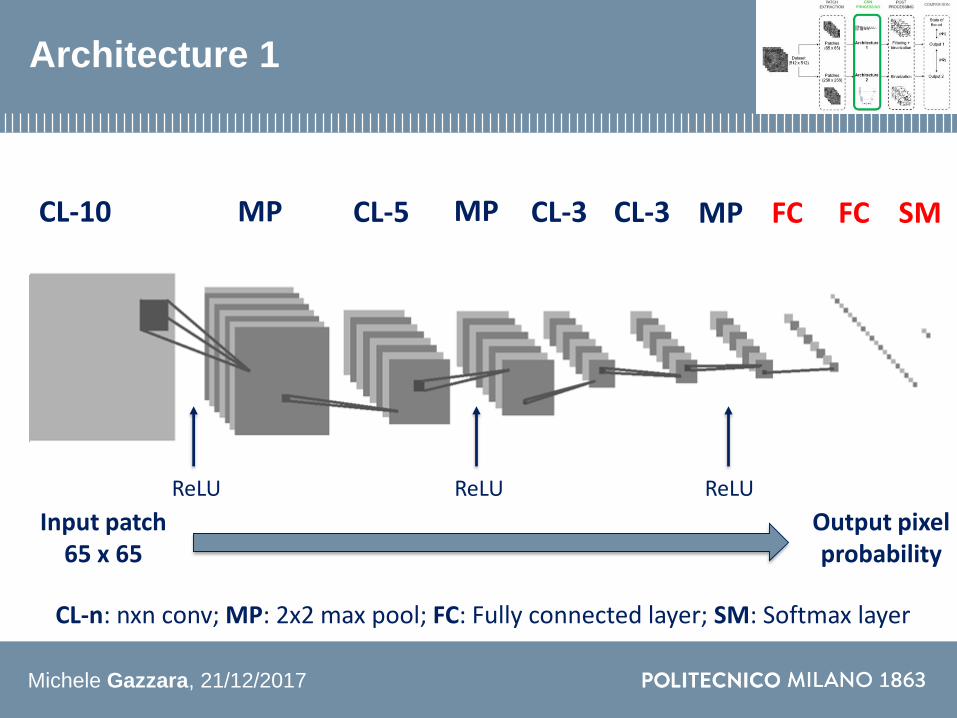
Michele Gazzara 21122017
Architecture 1
CL-10 CL-3CL-3MPCL-5MP MP FCFC SM
Input patch65 x 65
Output pixel probability
CL-n nxn conv MP 2x2 max pool FC Fully connected layer SM Softmax layer
ReLUReLU ReLU
Michele Gazzara 21122017 (16)
Fully connected and Softmax layers
As many FC output valuesas the number of classes
p119895 = 119890119911119895
σ119898=1119872 119890119911119898
j = 0 1 hellip M
Where119963119947 is the FC output
M is the number of classes
Michele Gazzara 21122017
Architecture 1
CL-10 CL-3CL-3MPCL-5MP MP FCFC SM
Input patch65 x 65
Output pixel probability
CL-n nxn conv MP 2x2 max pool FC Fully connected layer SM Softmax layer
ReLUReLU ReLU
Michele Gazzara 21122017
Architecture 2
Output patch probability map
216 x 216
Input patch
256 x 256
(17)
Michele Gazzara 21122017
Architecture 2
Output patch probability map
216 x 216
Input patch
256 x 256
(17)
Michele Gazzara 21122017 (18)
Up-convolution
1) Up-sampling
2) 2x2 convolution
[O Ronneberger et al 2015]
Michele Gazzara 21122017
Architecture 2
Output patch probability map
216 x 216
Input patch
256 x 256
Michele Gazzara 21122017
Training settings
Cross EntropyWhereN number of samplesi sample indexy sample labelp sample probability
J = minus1
119873σ119894=1119873 119910119894 119897119900119892 119901119894 + 1 minus 119910119894 ∙ 119897119900119892(1 minus 119901119894)
(19)
[D Kline et al 2005]
Michele Gazzara 21122017
Training settings
Cross EntropyWhereN number of samplesi sample indexy sample labelp sample probability
J = minus1
119873σ119894=1119873 119910119894 119897119900119892 119901119894 + 1 minus 119910119894 ∙ 119897119900119892(1 minus 119901119894)
Mini-batch gradient descent
θ = θ minus 120578 120571120579 119869 (120579 119909(119894119894+119899) 119901(119894119894+119899))
Where120520 learning raten batch sizex input sample
(19)
[D Kline et al 2005]
[M Li et al 2014]
Michele Gazzara 21122017
Training settings
Cross EntropyWhereN number of samplesi sample indexy sample labelp sample probability
J = minus1
119873σ119894=1119873 119910119894 119897119900119892 119901119894 + 1 minus 119910119894 ∙ 119897119900119892(1 minus 119901119894)
Mini-batch gradient descent
Adam Optimizer
θ = θ minus 120578 120571120579 119869 (120579 119909(119894119894+119899) 119901(119894119894+119899))
Where120520 learning raten batch sizex input sample
θ119905+1119896 = θ119905119896 minus120578
119907119905 119892119905119896 + 120598
∙ 119898119905(119892119905119896)
Wheret batch indexk node indexv uncentered variancem meang gradient of J
(19)
[D Kingma et al 2014]
[D Kline et al 2005]
[M Li et al 2014]
Michele Gazzara 21122017
Materials and methods - Post processing
(20)
Michele Gazzara 21122017
Post processing
Architecture 1
Pixel probability
Spatial imagereconstruction
Medianfiltering
Otsuthresholding
(21)
Michele Gazzara 21122017
Post processing
Architecture 1
Pixel probability
Spatial imagereconstruction
Medianfiltering
Otsuthresholding
(21)
Patch probability
map
Otsuthresholding
Architecture 2
Michele Gazzara 21122017
Materials and methods - Comparison
(22)
Michele Gazzara 21122017
Evaluation protocol - Metrics
Accuracy (Acc)
Pixel error (PE)
Sensitivity (Sn) and Specificity (Sp)
SoslashrensenndashDice coefficient (DSC)
Sn = TP
TP+FN
PE = 1 - Acc
119860119888119888 =1
Nσj=1N 119904119888119900119903119890119895 score = ൝
1 119894119891 yj= ොy1198950 119894119891 yj ne ොy119895
119863119878119862 =2 119879119875
119865119875 + 119865119873 + 2 119879119875
Sp = TN
TN+FP
Where
119962119946 sample label
ෝ119962119946 prediction
N number of samples
i semple index
TP true positives
FN false negatives
TN true negatives
FP false positives
(23)
[I Arganda-Carreras et al 2015]
Michele Gazzara 21122017
Evaluation protocol - H1 and H2
Investigation of H1
VSNon CNN-based approaches
CNN-based approaches
Architecture 1(PE)
(24)
Investigation of H2
Architecture 1(Performance metrics and
computational costs)
Architecture 2(Performance metrics and
computational costs)
VS(Lilliefors and Wilcoxon test)
Michele Gazzara 21122017
Results - Investigation of H1
Model Method PE [∙10minus3]
Architecture 1 CNN 88
Kaynig et al (2010) RF 157
Liu et al (2012) ANN 134
Model Training images Training time PE [∙10minus3]
Architecture 1 327680 5 hours 10 min 88
Ciresan et al (2012) 3 millions 85 hours 60
Fakhry et al (2015) 42 millions 30 hours 51
Comparison with non-CNN based models
Comparison with other CNN based models
(25)
PE = 1 - Acc
Michele Gazzara 21122017
Evaluation protocol - H1 and H2
Investigation of H1
VSNon CNN-based approaches
CNN-based approaches
Architecture 1(PE)
Investigation of H2
Architecture 1(Performance metrics and
computational costs)
Architecture 2(Performance metrics and
computational costs)
VS(Lilliefors and Wilcoxon test)
Michele Gazzara 21122017
Results - Investigation of H2 metrics
(26)
Michele Gazzara 21122017
Results - Investigation of H2 computational costs
(27)
Michele Gazzara 21122017
Results - Segmented images
Architecture 2 output
Architecture 1 output
Input image Ground truth
(28)
Michele Gazzara 21122017
Discussion
H1
1 Architecture 1 performances exceed the non CNN-based models
2 Architecture 1 performances are comparable with other CNN-based models
Reduced dataset and training time
(29)
Michele Gazzara 21122017
Discussion
H1
1 Architecture 1 performances exceed the non CNN-based models
2 Architecture 1 performances are comparable with other CNN-based models
Reduced dataset and training time
H2
1 Architecture 2 overcomes Architecture 1in terms of accuracy
2 Architecture 2 computational costs are lower than Architecture 1
Architecture 1detects more FPs
Architecture 2 can be used for real
time applications
(29)
Michele Gazzara 21122017
Conclusions and future work
CONCLUSIONS
Automatic method for axon segmentation in EM images
Performances comparable with existing CNN models
Reduced computational costs
(30)
Michele Gazzara 21122017
Conclusions and future work
CONCLUSIONS
Automatic method for axon segmentation in EM images
Performances comparable with existing CNN models
Reduced computational costs
FUTURE WORK
Larger dataset
Human brain EM images
Up-convolution improvement
(30)
[H Gao et al 2017]
Michele Gazzara 21122017
Acknowledgements
(31)
Michele Gazzara 21122017
Thank you for your attention
(32)

Michele Gazzara 21122017
Architecture 1
CL-10 CL-3CL-3MPCL-5MP MP FCFC SM
Input patch65 x 65
Output pixel probability
CL-n nxn conv MP 2x2 max pool FC Fully connected layer SM Softmax layer
ReLUReLU ReLU
Michele Gazzara 21122017
Architecture 2
Output patch probability map
216 x 216
Input patch
256 x 256
(17)
Michele Gazzara 21122017
Architecture 2
Output patch probability map
216 x 216
Input patch
256 x 256
(17)
Michele Gazzara 21122017 (18)
Up-convolution
1) Up-sampling
2) 2x2 convolution
[O Ronneberger et al 2015]
Michele Gazzara 21122017
Architecture 2
Output patch probability map
216 x 216
Input patch
256 x 256
Michele Gazzara 21122017
Training settings
Cross EntropyWhereN number of samplesi sample indexy sample labelp sample probability
J = minus1
119873σ119894=1119873 119910119894 119897119900119892 119901119894 + 1 minus 119910119894 ∙ 119897119900119892(1 minus 119901119894)
(19)
[D Kline et al 2005]
Michele Gazzara 21122017
Training settings
Cross EntropyWhereN number of samplesi sample indexy sample labelp sample probability
J = minus1
119873σ119894=1119873 119910119894 119897119900119892 119901119894 + 1 minus 119910119894 ∙ 119897119900119892(1 minus 119901119894)
Mini-batch gradient descent
θ = θ minus 120578 120571120579 119869 (120579 119909(119894119894+119899) 119901(119894119894+119899))
Where120520 learning raten batch sizex input sample
(19)
[D Kline et al 2005]
[M Li et al 2014]
Michele Gazzara 21122017
Training settings
Cross EntropyWhereN number of samplesi sample indexy sample labelp sample probability
J = minus1
119873σ119894=1119873 119910119894 119897119900119892 119901119894 + 1 minus 119910119894 ∙ 119897119900119892(1 minus 119901119894)
Mini-batch gradient descent
Adam Optimizer
θ = θ minus 120578 120571120579 119869 (120579 119909(119894119894+119899) 119901(119894119894+119899))
Where120520 learning raten batch sizex input sample
θ119905+1119896 = θ119905119896 minus120578
119907119905 119892119905119896 + 120598
∙ 119898119905(119892119905119896)
Wheret batch indexk node indexv uncentered variancem meang gradient of J
(19)
[D Kingma et al 2014]
[D Kline et al 2005]
[M Li et al 2014]
Michele Gazzara 21122017
Materials and methods - Post processing
(20)
Michele Gazzara 21122017
Post processing
Architecture 1
Pixel probability
Spatial imagereconstruction
Medianfiltering
Otsuthresholding
(21)
Michele Gazzara 21122017
Post processing
Architecture 1
Pixel probability
Spatial imagereconstruction
Medianfiltering
Otsuthresholding
(21)
Patch probability
map
Otsuthresholding
Architecture 2
Michele Gazzara 21122017
Materials and methods - Comparison
(22)
Michele Gazzara 21122017
Evaluation protocol - Metrics
Accuracy (Acc)
Pixel error (PE)
Sensitivity (Sn) and Specificity (Sp)
SoslashrensenndashDice coefficient (DSC)
Sn = TP
TP+FN
PE = 1 - Acc
119860119888119888 =1
Nσj=1N 119904119888119900119903119890119895 score = ൝
1 119894119891 yj= ොy1198950 119894119891 yj ne ොy119895
119863119878119862 =2 119879119875
119865119875 + 119865119873 + 2 119879119875
Sp = TN
TN+FP
Where
119962119946 sample label
ෝ119962119946 prediction
N number of samples
i semple index
TP true positives
FN false negatives
TN true negatives
FP false positives
(23)
[I Arganda-Carreras et al 2015]
Michele Gazzara 21122017
Evaluation protocol - H1 and H2
Investigation of H1
VSNon CNN-based approaches
CNN-based approaches
Architecture 1(PE)
(24)
Investigation of H2
Architecture 1(Performance metrics and
computational costs)
Architecture 2(Performance metrics and
computational costs)
VS(Lilliefors and Wilcoxon test)
Michele Gazzara 21122017
Results - Investigation of H1
Model Method PE [∙10minus3]
Architecture 1 CNN 88
Kaynig et al (2010) RF 157
Liu et al (2012) ANN 134
Model Training images Training time PE [∙10minus3]
Architecture 1 327680 5 hours 10 min 88
Ciresan et al (2012) 3 millions 85 hours 60
Fakhry et al (2015) 42 millions 30 hours 51
Comparison with non-CNN based models
Comparison with other CNN based models
(25)
PE = 1 - Acc
Michele Gazzara 21122017
Evaluation protocol - H1 and H2
Investigation of H1
VSNon CNN-based approaches
CNN-based approaches
Architecture 1(PE)
Investigation of H2
Architecture 1(Performance metrics and
computational costs)
Architecture 2(Performance metrics and
computational costs)
VS(Lilliefors and Wilcoxon test)
Michele Gazzara 21122017
Results - Investigation of H2 metrics
(26)
Michele Gazzara 21122017
Results - Investigation of H2 computational costs
(27)
Michele Gazzara 21122017
Results - Segmented images
Architecture 2 output
Architecture 1 output
Input image Ground truth
(28)
Michele Gazzara 21122017
Discussion
H1
1 Architecture 1 performances exceed the non CNN-based models
2 Architecture 1 performances are comparable with other CNN-based models
Reduced dataset and training time
(29)
Michele Gazzara 21122017
Discussion
H1
1 Architecture 1 performances exceed the non CNN-based models
2 Architecture 1 performances are comparable with other CNN-based models
Reduced dataset and training time
H2
1 Architecture 2 overcomes Architecture 1in terms of accuracy
2 Architecture 2 computational costs are lower than Architecture 1
Architecture 1detects more FPs
Architecture 2 can be used for real
time applications
(29)
Michele Gazzara 21122017
Conclusions and future work
CONCLUSIONS
Automatic method for axon segmentation in EM images
Performances comparable with existing CNN models
Reduced computational costs
(30)
Michele Gazzara 21122017
Conclusions and future work
CONCLUSIONS
Automatic method for axon segmentation in EM images
Performances comparable with existing CNN models
Reduced computational costs
FUTURE WORK
Larger dataset
Human brain EM images
Up-convolution improvement
(30)
[H Gao et al 2017]
Michele Gazzara 21122017
Acknowledgements
(31)
Michele Gazzara 21122017
Thank you for your attention
(32)

Michele Gazzara 21122017
Architecture 2
Output patch probability map
216 x 216
Input patch
256 x 256
(17)
Michele Gazzara 21122017
Architecture 2
Output patch probability map
216 x 216
Input patch
256 x 256
(17)
Michele Gazzara 21122017 (18)
Up-convolution
1) Up-sampling
2) 2x2 convolution
[O Ronneberger et al 2015]
Michele Gazzara 21122017
Architecture 2
Output patch probability map
216 x 216
Input patch
256 x 256
Michele Gazzara 21122017
Training settings
Cross EntropyWhereN number of samplesi sample indexy sample labelp sample probability
J = minus1
119873σ119894=1119873 119910119894 119897119900119892 119901119894 + 1 minus 119910119894 ∙ 119897119900119892(1 minus 119901119894)
(19)
[D Kline et al 2005]
Michele Gazzara 21122017
Training settings
Cross EntropyWhereN number of samplesi sample indexy sample labelp sample probability
J = minus1
119873σ119894=1119873 119910119894 119897119900119892 119901119894 + 1 minus 119910119894 ∙ 119897119900119892(1 minus 119901119894)
Mini-batch gradient descent
θ = θ minus 120578 120571120579 119869 (120579 119909(119894119894+119899) 119901(119894119894+119899))
Where120520 learning raten batch sizex input sample
(19)
[D Kline et al 2005]
[M Li et al 2014]
Michele Gazzara 21122017
Training settings
Cross EntropyWhereN number of samplesi sample indexy sample labelp sample probability
J = minus1
119873σ119894=1119873 119910119894 119897119900119892 119901119894 + 1 minus 119910119894 ∙ 119897119900119892(1 minus 119901119894)
Mini-batch gradient descent
Adam Optimizer
θ = θ minus 120578 120571120579 119869 (120579 119909(119894119894+119899) 119901(119894119894+119899))
Where120520 learning raten batch sizex input sample
θ119905+1119896 = θ119905119896 minus120578
119907119905 119892119905119896 + 120598
∙ 119898119905(119892119905119896)
Wheret batch indexk node indexv uncentered variancem meang gradient of J
(19)
[D Kingma et al 2014]
[D Kline et al 2005]
[M Li et al 2014]
Michele Gazzara 21122017
Materials and methods - Post processing
(20)
Michele Gazzara 21122017
Post processing
Architecture 1
Pixel probability
Spatial imagereconstruction
Medianfiltering
Otsuthresholding
(21)
Michele Gazzara 21122017
Post processing
Architecture 1
Pixel probability
Spatial imagereconstruction
Medianfiltering
Otsuthresholding
(21)
Patch probability
map
Otsuthresholding
Architecture 2
Michele Gazzara 21122017
Materials and methods - Comparison
(22)
Michele Gazzara 21122017
Evaluation protocol - Metrics
Accuracy (Acc)
Pixel error (PE)
Sensitivity (Sn) and Specificity (Sp)
SoslashrensenndashDice coefficient (DSC)
Sn = TP
TP+FN
PE = 1 - Acc
119860119888119888 =1
Nσj=1N 119904119888119900119903119890119895 score = ൝
1 119894119891 yj= ොy1198950 119894119891 yj ne ොy119895
119863119878119862 =2 119879119875
119865119875 + 119865119873 + 2 119879119875
Sp = TN
TN+FP
Where
119962119946 sample label
ෝ119962119946 prediction
N number of samples
i semple index
TP true positives
FN false negatives
TN true negatives
FP false positives
(23)
[I Arganda-Carreras et al 2015]
Michele Gazzara 21122017
Evaluation protocol - H1 and H2
Investigation of H1
VSNon CNN-based approaches
CNN-based approaches
Architecture 1(PE)
(24)
Investigation of H2
Architecture 1(Performance metrics and
computational costs)
Architecture 2(Performance metrics and
computational costs)
VS(Lilliefors and Wilcoxon test)
Michele Gazzara 21122017
Results - Investigation of H1
Model Method PE [∙10minus3]
Architecture 1 CNN 88
Kaynig et al (2010) RF 157
Liu et al (2012) ANN 134
Model Training images Training time PE [∙10minus3]
Architecture 1 327680 5 hours 10 min 88
Ciresan et al (2012) 3 millions 85 hours 60
Fakhry et al (2015) 42 millions 30 hours 51
Comparison with non-CNN based models
Comparison with other CNN based models
(25)
PE = 1 - Acc
Michele Gazzara 21122017
Evaluation protocol - H1 and H2
Investigation of H1
VSNon CNN-based approaches
CNN-based approaches
Architecture 1(PE)
Investigation of H2
Architecture 1(Performance metrics and
computational costs)
Architecture 2(Performance metrics and
computational costs)
VS(Lilliefors and Wilcoxon test)
Michele Gazzara 21122017
Results - Investigation of H2 metrics
(26)
Michele Gazzara 21122017
Results - Investigation of H2 computational costs
(27)
Michele Gazzara 21122017
Results - Segmented images
Architecture 2 output
Architecture 1 output
Input image Ground truth
(28)
Michele Gazzara 21122017
Discussion
H1
1 Architecture 1 performances exceed the non CNN-based models
2 Architecture 1 performances are comparable with other CNN-based models
Reduced dataset and training time
(29)
Michele Gazzara 21122017
Discussion
H1
1 Architecture 1 performances exceed the non CNN-based models
2 Architecture 1 performances are comparable with other CNN-based models
Reduced dataset and training time
H2
1 Architecture 2 overcomes Architecture 1in terms of accuracy
2 Architecture 2 computational costs are lower than Architecture 1
Architecture 1detects more FPs
Architecture 2 can be used for real
time applications
(29)
Michele Gazzara 21122017
Conclusions and future work
CONCLUSIONS
Automatic method for axon segmentation in EM images
Performances comparable with existing CNN models
Reduced computational costs
(30)
Michele Gazzara 21122017
Conclusions and future work
CONCLUSIONS
Automatic method for axon segmentation in EM images
Performances comparable with existing CNN models
Reduced computational costs
FUTURE WORK
Larger dataset
Human brain EM images
Up-convolution improvement
(30)
[H Gao et al 2017]
Michele Gazzara 21122017
Acknowledgements
(31)
Michele Gazzara 21122017
Thank you for your attention
(32)
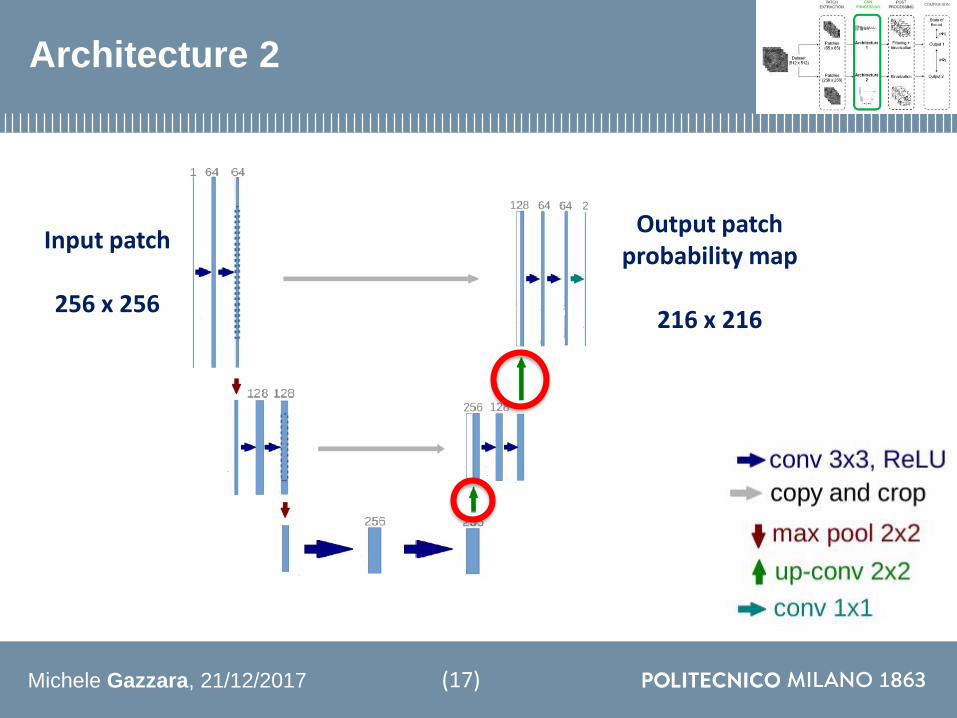
Michele Gazzara 21122017
Architecture 2
Output patch probability map
216 x 216
Input patch
256 x 256
(17)
Michele Gazzara 21122017 (18)
Up-convolution
1) Up-sampling
2) 2x2 convolution
[O Ronneberger et al 2015]
Michele Gazzara 21122017
Architecture 2
Output patch probability map
216 x 216
Input patch
256 x 256
Michele Gazzara 21122017
Training settings
Cross EntropyWhereN number of samplesi sample indexy sample labelp sample probability
J = minus1
119873σ119894=1119873 119910119894 119897119900119892 119901119894 + 1 minus 119910119894 ∙ 119897119900119892(1 minus 119901119894)
(19)
[D Kline et al 2005]
Michele Gazzara 21122017
Training settings
Cross EntropyWhereN number of samplesi sample indexy sample labelp sample probability
J = minus1
119873σ119894=1119873 119910119894 119897119900119892 119901119894 + 1 minus 119910119894 ∙ 119897119900119892(1 minus 119901119894)
Mini-batch gradient descent
θ = θ minus 120578 120571120579 119869 (120579 119909(119894119894+119899) 119901(119894119894+119899))
Where120520 learning raten batch sizex input sample
(19)
[D Kline et al 2005]
[M Li et al 2014]
Michele Gazzara 21122017
Training settings
Cross EntropyWhereN number of samplesi sample indexy sample labelp sample probability
J = minus1
119873σ119894=1119873 119910119894 119897119900119892 119901119894 + 1 minus 119910119894 ∙ 119897119900119892(1 minus 119901119894)
Mini-batch gradient descent
Adam Optimizer
θ = θ minus 120578 120571120579 119869 (120579 119909(119894119894+119899) 119901(119894119894+119899))
Where120520 learning raten batch sizex input sample
θ119905+1119896 = θ119905119896 minus120578
119907119905 119892119905119896 + 120598
∙ 119898119905(119892119905119896)
Wheret batch indexk node indexv uncentered variancem meang gradient of J
(19)
[D Kingma et al 2014]
[D Kline et al 2005]
[M Li et al 2014]
Michele Gazzara 21122017
Materials and methods - Post processing
(20)
Michele Gazzara 21122017
Post processing
Architecture 1
Pixel probability
Spatial imagereconstruction
Medianfiltering
Otsuthresholding
(21)
Michele Gazzara 21122017
Post processing
Architecture 1
Pixel probability
Spatial imagereconstruction
Medianfiltering
Otsuthresholding
(21)
Patch probability
map
Otsuthresholding
Architecture 2
Michele Gazzara 21122017
Materials and methods - Comparison
(22)
Michele Gazzara 21122017
Evaluation protocol - Metrics
Accuracy (Acc)
Pixel error (PE)
Sensitivity (Sn) and Specificity (Sp)
SoslashrensenndashDice coefficient (DSC)
Sn = TP
TP+FN
PE = 1 - Acc
119860119888119888 =1
Nσj=1N 119904119888119900119903119890119895 score = ൝
1 119894119891 yj= ොy1198950 119894119891 yj ne ොy119895
119863119878119862 =2 119879119875
119865119875 + 119865119873 + 2 119879119875
Sp = TN
TN+FP
Where
119962119946 sample label
ෝ119962119946 prediction
N number of samples
i semple index
TP true positives
FN false negatives
TN true negatives
FP false positives
(23)
[I Arganda-Carreras et al 2015]
Michele Gazzara 21122017
Evaluation protocol - H1 and H2
Investigation of H1
VSNon CNN-based approaches
CNN-based approaches
Architecture 1(PE)
(24)
Investigation of H2
Architecture 1(Performance metrics and
computational costs)
Architecture 2(Performance metrics and
computational costs)
VS(Lilliefors and Wilcoxon test)
Michele Gazzara 21122017
Results - Investigation of H1
Model Method PE [∙10minus3]
Architecture 1 CNN 88
Kaynig et al (2010) RF 157
Liu et al (2012) ANN 134
Model Training images Training time PE [∙10minus3]
Architecture 1 327680 5 hours 10 min 88
Ciresan et al (2012) 3 millions 85 hours 60
Fakhry et al (2015) 42 millions 30 hours 51
Comparison with non-CNN based models
Comparison with other CNN based models
(25)
PE = 1 - Acc
Michele Gazzara 21122017
Evaluation protocol - H1 and H2
Investigation of H1
VSNon CNN-based approaches
CNN-based approaches
Architecture 1(PE)
Investigation of H2
Architecture 1(Performance metrics and
computational costs)
Architecture 2(Performance metrics and
computational costs)
VS(Lilliefors and Wilcoxon test)
Michele Gazzara 21122017
Results - Investigation of H2 metrics
(26)
Michele Gazzara 21122017
Results - Investigation of H2 computational costs
(27)
Michele Gazzara 21122017
Results - Segmented images
Architecture 2 output
Architecture 1 output
Input image Ground truth
(28)
Michele Gazzara 21122017
Discussion
H1
1 Architecture 1 performances exceed the non CNN-based models
2 Architecture 1 performances are comparable with other CNN-based models
Reduced dataset and training time
(29)
Michele Gazzara 21122017
Discussion
H1
1 Architecture 1 performances exceed the non CNN-based models
2 Architecture 1 performances are comparable with other CNN-based models
Reduced dataset and training time
H2
1 Architecture 2 overcomes Architecture 1in terms of accuracy
2 Architecture 2 computational costs are lower than Architecture 1
Architecture 1detects more FPs
Architecture 2 can be used for real
time applications
(29)
Michele Gazzara 21122017
Conclusions and future work
CONCLUSIONS
Automatic method for axon segmentation in EM images
Performances comparable with existing CNN models
Reduced computational costs
(30)
Michele Gazzara 21122017
Conclusions and future work
CONCLUSIONS
Automatic method for axon segmentation in EM images
Performances comparable with existing CNN models
Reduced computational costs
FUTURE WORK
Larger dataset
Human brain EM images
Up-convolution improvement
(30)
[H Gao et al 2017]
Michele Gazzara 21122017
Acknowledgements
(31)
Michele Gazzara 21122017
Thank you for your attention
(32)
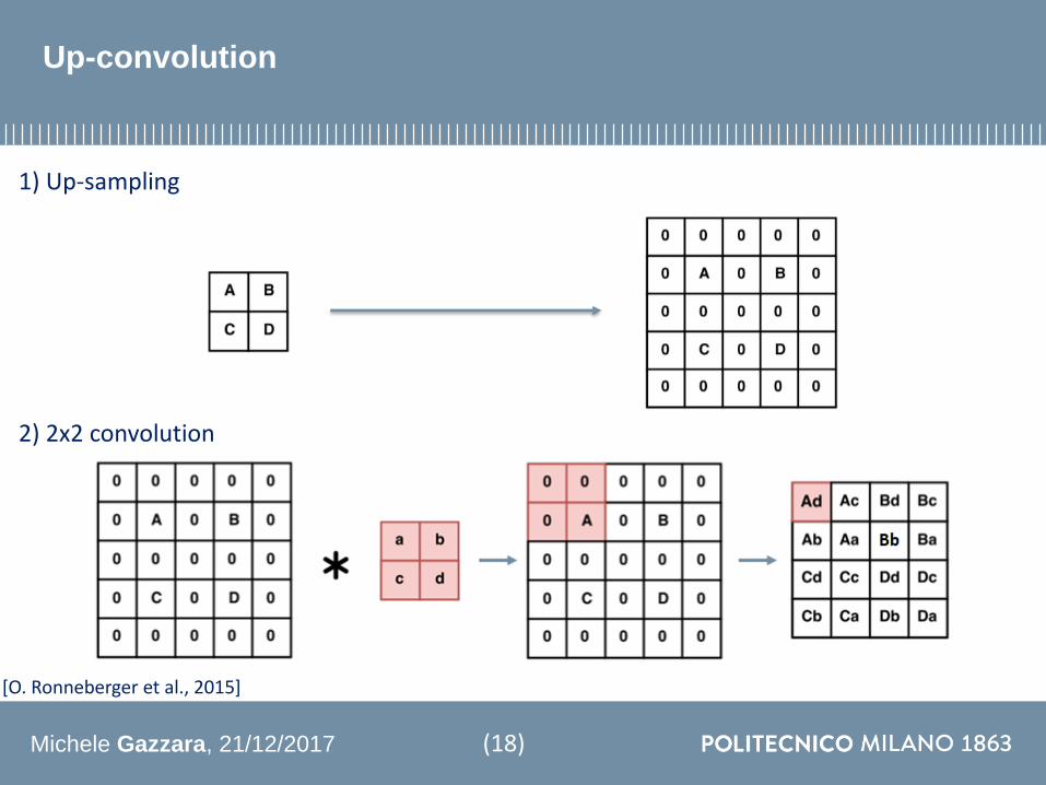

Michele Gazzara 21122017
Architecture 2
Output patch probability map
216 x 216
Input patch
256 x 256
Michele Gazzara 21122017
Training settings
Cross EntropyWhereN number of samplesi sample indexy sample labelp sample probability
J = minus1
119873σ119894=1119873 119910119894 119897119900119892 119901119894 + 1 minus 119910119894 ∙ 119897119900119892(1 minus 119901119894)
(19)
[D Kline et al 2005]
Michele Gazzara 21122017
Training settings
Cross EntropyWhereN number of samplesi sample indexy sample labelp sample probability
J = minus1
119873σ119894=1119873 119910119894 119897119900119892 119901119894 + 1 minus 119910119894 ∙ 119897119900119892(1 minus 119901119894)
Mini-batch gradient descent
θ = θ minus 120578 120571120579 119869 (120579 119909(119894119894+119899) 119901(119894119894+119899))
Where120520 learning raten batch sizex input sample
(19)
[D Kline et al 2005]
[M Li et al 2014]
Michele Gazzara 21122017
Training settings
Cross EntropyWhereN number of samplesi sample indexy sample labelp sample probability
J = minus1
119873σ119894=1119873 119910119894 119897119900119892 119901119894 + 1 minus 119910119894 ∙ 119897119900119892(1 minus 119901119894)
Mini-batch gradient descent
Adam Optimizer
θ = θ minus 120578 120571120579 119869 (120579 119909(119894119894+119899) 119901(119894119894+119899))
Where120520 learning raten batch sizex input sample
θ119905+1119896 = θ119905119896 minus120578
119907119905 119892119905119896 + 120598
∙ 119898119905(119892119905119896)
Wheret batch indexk node indexv uncentered variancem meang gradient of J
(19)
[D Kingma et al 2014]
[D Kline et al 2005]
[M Li et al 2014]
Michele Gazzara 21122017
Materials and methods - Post processing
(20)
Michele Gazzara 21122017
Post processing
Architecture 1
Pixel probability
Spatial imagereconstruction
Medianfiltering
Otsuthresholding
(21)
Michele Gazzara 21122017
Post processing
Architecture 1
Pixel probability
Spatial imagereconstruction
Medianfiltering
Otsuthresholding
(21)
Patch probability
map
Otsuthresholding
Architecture 2
Michele Gazzara 21122017
Materials and methods - Comparison
(22)
Michele Gazzara 21122017
Evaluation protocol - Metrics
Accuracy (Acc)
Pixel error (PE)
Sensitivity (Sn) and Specificity (Sp)
SoslashrensenndashDice coefficient (DSC)
Sn = TP
TP+FN
PE = 1 - Acc
119860119888119888 =1
Nσj=1N 119904119888119900119903119890119895 score = ൝
1 119894119891 yj= ොy1198950 119894119891 yj ne ොy119895
119863119878119862 =2 119879119875
119865119875 + 119865119873 + 2 119879119875
Sp = TN
TN+FP
Where
119962119946 sample label
ෝ119962119946 prediction
N number of samples
i semple index
TP true positives
FN false negatives
TN true negatives
FP false positives
(23)
[I Arganda-Carreras et al 2015]
Michele Gazzara 21122017
Evaluation protocol - H1 and H2
Investigation of H1
VSNon CNN-based approaches
CNN-based approaches
Architecture 1(PE)
(24)
Investigation of H2
Architecture 1(Performance metrics and
computational costs)
Architecture 2(Performance metrics and
computational costs)
VS(Lilliefors and Wilcoxon test)
Michele Gazzara 21122017
Results - Investigation of H1
Model Method PE [∙10minus3]
Architecture 1 CNN 88
Kaynig et al (2010) RF 157
Liu et al (2012) ANN 134
Model Training images Training time PE [∙10minus3]
Architecture 1 327680 5 hours 10 min 88
Ciresan et al (2012) 3 millions 85 hours 60
Fakhry et al (2015) 42 millions 30 hours 51
Comparison with non-CNN based models
Comparison with other CNN based models
(25)
PE = 1 - Acc
Michele Gazzara 21122017
Evaluation protocol - H1 and H2
Investigation of H1
VSNon CNN-based approaches
CNN-based approaches
Architecture 1(PE)
Investigation of H2
Architecture 1(Performance metrics and
computational costs)
Architecture 2(Performance metrics and
computational costs)
VS(Lilliefors and Wilcoxon test)
Michele Gazzara 21122017
Results - Investigation of H2 metrics
(26)
Michele Gazzara 21122017
Results - Investigation of H2 computational costs
(27)
Michele Gazzara 21122017
Results - Segmented images
Architecture 2 output
Architecture 1 output
Input image Ground truth
(28)
Michele Gazzara 21122017
Discussion
H1
1 Architecture 1 performances exceed the non CNN-based models
2 Architecture 1 performances are comparable with other CNN-based models
Reduced dataset and training time
(29)
Michele Gazzara 21122017
Discussion
H1
1 Architecture 1 performances exceed the non CNN-based models
2 Architecture 1 performances are comparable with other CNN-based models
Reduced dataset and training time
H2
1 Architecture 2 overcomes Architecture 1in terms of accuracy
2 Architecture 2 computational costs are lower than Architecture 1
Architecture 1detects more FPs
Architecture 2 can be used for real
time applications
(29)
Michele Gazzara 21122017
Conclusions and future work
CONCLUSIONS
Automatic method for axon segmentation in EM images
Performances comparable with existing CNN models
Reduced computational costs
(30)
Michele Gazzara 21122017
Conclusions and future work
CONCLUSIONS
Automatic method for axon segmentation in EM images
Performances comparable with existing CNN models
Reduced computational costs
FUTURE WORK
Larger dataset
Human brain EM images
Up-convolution improvement
(30)
[H Gao et al 2017]
Michele Gazzara 21122017
Acknowledgements
(31)
Michele Gazzara 21122017
Thank you for your attention
(32)
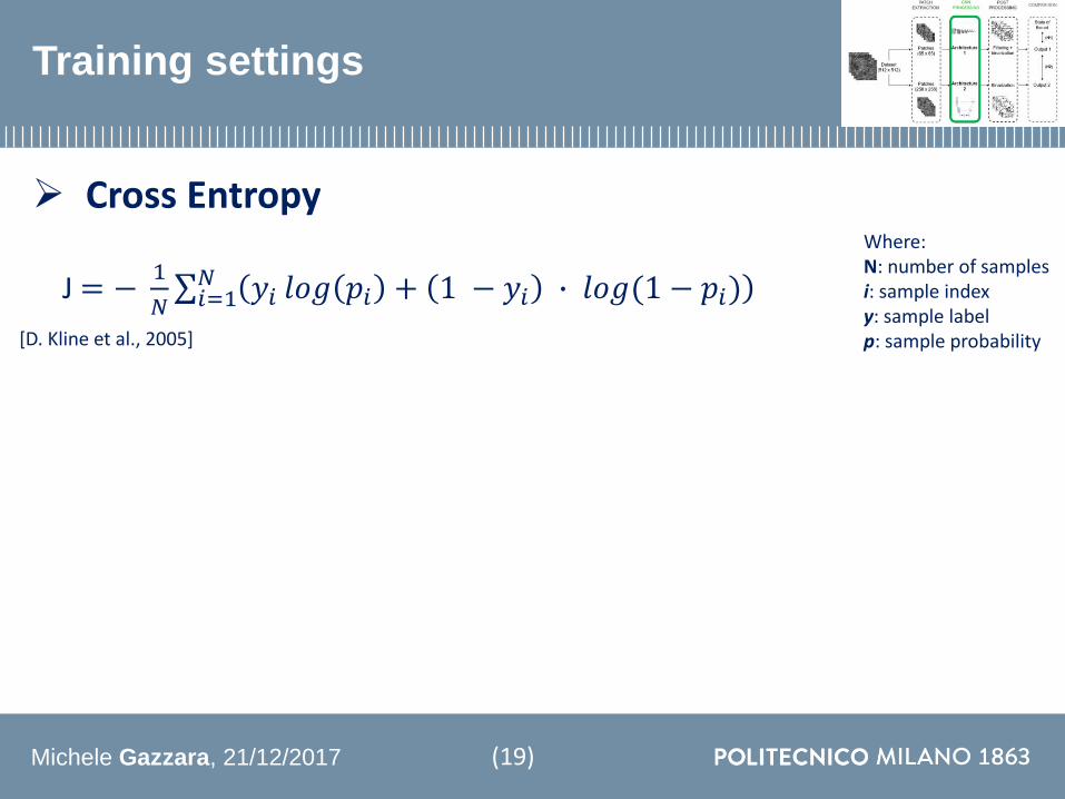
Michele Gazzara 21122017
Training settings
Cross EntropyWhereN number of samplesi sample indexy sample labelp sample probability
J = minus1
119873σ119894=1119873 119910119894 119897119900119892 119901119894 + 1 minus 119910119894 ∙ 119897119900119892(1 minus 119901119894)
(19)
[D Kline et al 2005]
Michele Gazzara 21122017
Training settings
Cross EntropyWhereN number of samplesi sample indexy sample labelp sample probability
J = minus1
119873σ119894=1119873 119910119894 119897119900119892 119901119894 + 1 minus 119910119894 ∙ 119897119900119892(1 minus 119901119894)
Mini-batch gradient descent
θ = θ minus 120578 120571120579 119869 (120579 119909(119894119894+119899) 119901(119894119894+119899))
Where120520 learning raten batch sizex input sample
(19)
[D Kline et al 2005]
[M Li et al 2014]
Michele Gazzara 21122017
Training settings
Cross EntropyWhereN number of samplesi sample indexy sample labelp sample probability
J = minus1
119873σ119894=1119873 119910119894 119897119900119892 119901119894 + 1 minus 119910119894 ∙ 119897119900119892(1 minus 119901119894)
Mini-batch gradient descent
Adam Optimizer
θ = θ minus 120578 120571120579 119869 (120579 119909(119894119894+119899) 119901(119894119894+119899))
Where120520 learning raten batch sizex input sample
θ119905+1119896 = θ119905119896 minus120578
119907119905 119892119905119896 + 120598
∙ 119898119905(119892119905119896)
Wheret batch indexk node indexv uncentered variancem meang gradient of J
(19)
[D Kingma et al 2014]
[D Kline et al 2005]
[M Li et al 2014]
Michele Gazzara 21122017
Materials and methods - Post processing
(20)
Michele Gazzara 21122017
Post processing
Architecture 1
Pixel probability
Spatial imagereconstruction
Medianfiltering
Otsuthresholding
(21)
Michele Gazzara 21122017
Post processing
Architecture 1
Pixel probability
Spatial imagereconstruction
Medianfiltering
Otsuthresholding
(21)
Patch probability
map
Otsuthresholding
Architecture 2
Michele Gazzara 21122017
Materials and methods - Comparison
(22)
Michele Gazzara 21122017
Evaluation protocol - Metrics
Accuracy (Acc)
Pixel error (PE)
Sensitivity (Sn) and Specificity (Sp)
SoslashrensenndashDice coefficient (DSC)
Sn = TP
TP+FN
PE = 1 - Acc
119860119888119888 =1
Nσj=1N 119904119888119900119903119890119895 score = ൝
1 119894119891 yj= ොy1198950 119894119891 yj ne ොy119895
119863119878119862 =2 119879119875
119865119875 + 119865119873 + 2 119879119875
Sp = TN
TN+FP
Where
119962119946 sample label
ෝ119962119946 prediction
N number of samples
i semple index
TP true positives
FN false negatives
TN true negatives
FP false positives
(23)
[I Arganda-Carreras et al 2015]
Michele Gazzara 21122017
Evaluation protocol - H1 and H2
Investigation of H1
VSNon CNN-based approaches
CNN-based approaches
Architecture 1(PE)
(24)
Investigation of H2
Architecture 1(Performance metrics and
computational costs)
Architecture 2(Performance metrics and
computational costs)
VS(Lilliefors and Wilcoxon test)
Michele Gazzara 21122017
Results - Investigation of H1
Model Method PE [∙10minus3]
Architecture 1 CNN 88
Kaynig et al (2010) RF 157
Liu et al (2012) ANN 134
Model Training images Training time PE [∙10minus3]
Architecture 1 327680 5 hours 10 min 88
Ciresan et al (2012) 3 millions 85 hours 60
Fakhry et al (2015) 42 millions 30 hours 51
Comparison with non-CNN based models
Comparison with other CNN based models
(25)
PE = 1 - Acc
Michele Gazzara 21122017
Evaluation protocol - H1 and H2
Investigation of H1
VSNon CNN-based approaches
CNN-based approaches
Architecture 1(PE)
Investigation of H2
Architecture 1(Performance metrics and
computational costs)
Architecture 2(Performance metrics and
computational costs)
VS(Lilliefors and Wilcoxon test)
Michele Gazzara 21122017
Results - Investigation of H2 metrics
(26)
Michele Gazzara 21122017
Results - Investigation of H2 computational costs
(27)
Michele Gazzara 21122017
Results - Segmented images
Architecture 2 output
Architecture 1 output
Input image Ground truth
(28)
Michele Gazzara 21122017
Discussion
H1
1 Architecture 1 performances exceed the non CNN-based models
2 Architecture 1 performances are comparable with other CNN-based models
Reduced dataset and training time
(29)
Michele Gazzara 21122017
Discussion
H1
1 Architecture 1 performances exceed the non CNN-based models
2 Architecture 1 performances are comparable with other CNN-based models
Reduced dataset and training time
H2
1 Architecture 2 overcomes Architecture 1in terms of accuracy
2 Architecture 2 computational costs are lower than Architecture 1
Architecture 1detects more FPs
Architecture 2 can be used for real
time applications
(29)
Michele Gazzara 21122017
Conclusions and future work
CONCLUSIONS
Automatic method for axon segmentation in EM images
Performances comparable with existing CNN models
Reduced computational costs
(30)
Michele Gazzara 21122017
Conclusions and future work
CONCLUSIONS
Automatic method for axon segmentation in EM images
Performances comparable with existing CNN models
Reduced computational costs
FUTURE WORK
Larger dataset
Human brain EM images
Up-convolution improvement
(30)
[H Gao et al 2017]
Michele Gazzara 21122017
Acknowledgements
(31)
Michele Gazzara 21122017
Thank you for your attention
(32)
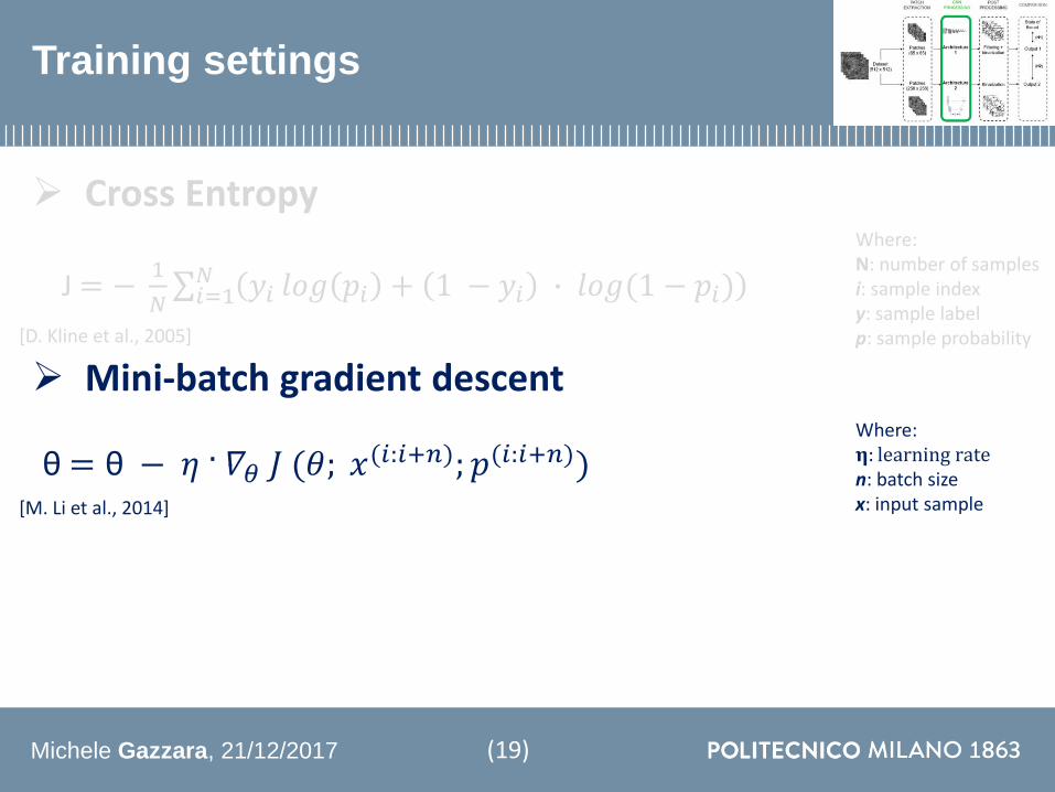
Michele Gazzara 21122017
Training settings
Cross EntropyWhereN number of samplesi sample indexy sample labelp sample probability
J = minus1
119873σ119894=1119873 119910119894 119897119900119892 119901119894 + 1 minus 119910119894 ∙ 119897119900119892(1 minus 119901119894)
Mini-batch gradient descent
θ = θ minus 120578 120571120579 119869 (120579 119909(119894119894+119899) 119901(119894119894+119899))
Where120520 learning raten batch sizex input sample
(19)
[D Kline et al 2005]
[M Li et al 2014]
Michele Gazzara 21122017
Training settings
Cross EntropyWhereN number of samplesi sample indexy sample labelp sample probability
J = minus1
119873σ119894=1119873 119910119894 119897119900119892 119901119894 + 1 minus 119910119894 ∙ 119897119900119892(1 minus 119901119894)
Mini-batch gradient descent
Adam Optimizer
θ = θ minus 120578 120571120579 119869 (120579 119909(119894119894+119899) 119901(119894119894+119899))
Where120520 learning raten batch sizex input sample
θ119905+1119896 = θ119905119896 minus120578
119907119905 119892119905119896 + 120598
∙ 119898119905(119892119905119896)
Wheret batch indexk node indexv uncentered variancem meang gradient of J
(19)
[D Kingma et al 2014]
[D Kline et al 2005]
[M Li et al 2014]
Michele Gazzara 21122017
Materials and methods - Post processing
(20)
Michele Gazzara 21122017
Post processing
Architecture 1
Pixel probability
Spatial imagereconstruction
Medianfiltering
Otsuthresholding
(21)
Michele Gazzara 21122017
Post processing
Architecture 1
Pixel probability
Spatial imagereconstruction
Medianfiltering
Otsuthresholding
(21)
Patch probability
map
Otsuthresholding
Architecture 2
Michele Gazzara 21122017
Materials and methods - Comparison
(22)
Michele Gazzara 21122017
Evaluation protocol - Metrics
Accuracy (Acc)
Pixel error (PE)
Sensitivity (Sn) and Specificity (Sp)
SoslashrensenndashDice coefficient (DSC)
Sn = TP
TP+FN
PE = 1 - Acc
119860119888119888 =1
Nσj=1N 119904119888119900119903119890119895 score = ൝
1 119894119891 yj= ොy1198950 119894119891 yj ne ොy119895
119863119878119862 =2 119879119875
119865119875 + 119865119873 + 2 119879119875
Sp = TN
TN+FP
Where
119962119946 sample label
ෝ119962119946 prediction
N number of samples
i semple index
TP true positives
FN false negatives
TN true negatives
FP false positives
(23)
[I Arganda-Carreras et al 2015]
Michele Gazzara 21122017
Evaluation protocol - H1 and H2
Investigation of H1
VSNon CNN-based approaches
CNN-based approaches
Architecture 1(PE)
(24)
Investigation of H2
Architecture 1(Performance metrics and
computational costs)
Architecture 2(Performance metrics and
computational costs)
VS(Lilliefors and Wilcoxon test)
Michele Gazzara 21122017
Results - Investigation of H1
Model Method PE [∙10minus3]
Architecture 1 CNN 88
Kaynig et al (2010) RF 157
Liu et al (2012) ANN 134
Model Training images Training time PE [∙10minus3]
Architecture 1 327680 5 hours 10 min 88
Ciresan et al (2012) 3 millions 85 hours 60
Fakhry et al (2015) 42 millions 30 hours 51
Comparison with non-CNN based models
Comparison with other CNN based models
(25)
PE = 1 - Acc
Michele Gazzara 21122017
Evaluation protocol - H1 and H2
Investigation of H1
VSNon CNN-based approaches
CNN-based approaches
Architecture 1(PE)
Investigation of H2
Architecture 1(Performance metrics and
computational costs)
Architecture 2(Performance metrics and
computational costs)
VS(Lilliefors and Wilcoxon test)
Michele Gazzara 21122017
Results - Investigation of H2 metrics
(26)
Michele Gazzara 21122017
Results - Investigation of H2 computational costs
(27)
Michele Gazzara 21122017
Results - Segmented images
Architecture 2 output
Architecture 1 output
Input image Ground truth
(28)
Michele Gazzara 21122017
Discussion
H1
1 Architecture 1 performances exceed the non CNN-based models
2 Architecture 1 performances are comparable with other CNN-based models
Reduced dataset and training time
(29)
Michele Gazzara 21122017
Discussion
H1
1 Architecture 1 performances exceed the non CNN-based models
2 Architecture 1 performances are comparable with other CNN-based models
Reduced dataset and training time
H2
1 Architecture 2 overcomes Architecture 1in terms of accuracy
2 Architecture 2 computational costs are lower than Architecture 1
Architecture 1detects more FPs
Architecture 2 can be used for real
time applications
(29)
Michele Gazzara 21122017
Conclusions and future work
CONCLUSIONS
Automatic method for axon segmentation in EM images
Performances comparable with existing CNN models
Reduced computational costs
(30)
Michele Gazzara 21122017
Conclusions and future work
CONCLUSIONS
Automatic method for axon segmentation in EM images
Performances comparable with existing CNN models
Reduced computational costs
FUTURE WORK
Larger dataset
Human brain EM images
Up-convolution improvement
(30)
[H Gao et al 2017]
Michele Gazzara 21122017
Acknowledgements
(31)
Michele Gazzara 21122017
Thank you for your attention
(32)

Michele Gazzara 21122017
Training settings
Cross EntropyWhereN number of samplesi sample indexy sample labelp sample probability
J = minus1
119873σ119894=1119873 119910119894 119897119900119892 119901119894 + 1 minus 119910119894 ∙ 119897119900119892(1 minus 119901119894)
Mini-batch gradient descent
Adam Optimizer
θ = θ minus 120578 120571120579 119869 (120579 119909(119894119894+119899) 119901(119894119894+119899))
Where120520 learning raten batch sizex input sample
θ119905+1119896 = θ119905119896 minus120578
119907119905 119892119905119896 + 120598
∙ 119898119905(119892119905119896)
Wheret batch indexk node indexv uncentered variancem meang gradient of J
(19)
[D Kingma et al 2014]
[D Kline et al 2005]
[M Li et al 2014]
Michele Gazzara 21122017
Materials and methods - Post processing
(20)
Michele Gazzara 21122017
Post processing
Architecture 1
Pixel probability
Spatial imagereconstruction
Medianfiltering
Otsuthresholding
(21)
Michele Gazzara 21122017
Post processing
Architecture 1
Pixel probability
Spatial imagereconstruction
Medianfiltering
Otsuthresholding
(21)
Patch probability
map
Otsuthresholding
Architecture 2
Michele Gazzara 21122017
Materials and methods - Comparison
(22)
Michele Gazzara 21122017
Evaluation protocol - Metrics
Accuracy (Acc)
Pixel error (PE)
Sensitivity (Sn) and Specificity (Sp)
SoslashrensenndashDice coefficient (DSC)
Sn = TP
TP+FN
PE = 1 - Acc
119860119888119888 =1
Nσj=1N 119904119888119900119903119890119895 score = ൝
1 119894119891 yj= ොy1198950 119894119891 yj ne ොy119895
119863119878119862 =2 119879119875
119865119875 + 119865119873 + 2 119879119875
Sp = TN
TN+FP
Where
119962119946 sample label
ෝ119962119946 prediction
N number of samples
i semple index
TP true positives
FN false negatives
TN true negatives
FP false positives
(23)
[I Arganda-Carreras et al 2015]
Michele Gazzara 21122017
Evaluation protocol - H1 and H2
Investigation of H1
VSNon CNN-based approaches
CNN-based approaches
Architecture 1(PE)
(24)
Investigation of H2
Architecture 1(Performance metrics and
computational costs)
Architecture 2(Performance metrics and
computational costs)
VS(Lilliefors and Wilcoxon test)
Michele Gazzara 21122017
Results - Investigation of H1
Model Method PE [∙10minus3]
Architecture 1 CNN 88
Kaynig et al (2010) RF 157
Liu et al (2012) ANN 134
Model Training images Training time PE [∙10minus3]
Architecture 1 327680 5 hours 10 min 88
Ciresan et al (2012) 3 millions 85 hours 60
Fakhry et al (2015) 42 millions 30 hours 51
Comparison with non-CNN based models
Comparison with other CNN based models
(25)
PE = 1 - Acc
Michele Gazzara 21122017
Evaluation protocol - H1 and H2
Investigation of H1
VSNon CNN-based approaches
CNN-based approaches
Architecture 1(PE)
Investigation of H2
Architecture 1(Performance metrics and
computational costs)
Architecture 2(Performance metrics and
computational costs)
VS(Lilliefors and Wilcoxon test)
Michele Gazzara 21122017
Results - Investigation of H2 metrics
(26)
Michele Gazzara 21122017
Results - Investigation of H2 computational costs
(27)
Michele Gazzara 21122017
Results - Segmented images
Architecture 2 output
Architecture 1 output
Input image Ground truth
(28)
Michele Gazzara 21122017
Discussion
H1
1 Architecture 1 performances exceed the non CNN-based models
2 Architecture 1 performances are comparable with other CNN-based models
Reduced dataset and training time
(29)
Michele Gazzara 21122017
Discussion
H1
1 Architecture 1 performances exceed the non CNN-based models
2 Architecture 1 performances are comparable with other CNN-based models
Reduced dataset and training time
H2
1 Architecture 2 overcomes Architecture 1in terms of accuracy
2 Architecture 2 computational costs are lower than Architecture 1
Architecture 1detects more FPs
Architecture 2 can be used for real
time applications
(29)
Michele Gazzara 21122017
Conclusions and future work
CONCLUSIONS
Automatic method for axon segmentation in EM images
Performances comparable with existing CNN models
Reduced computational costs
(30)
Michele Gazzara 21122017
Conclusions and future work
CONCLUSIONS
Automatic method for axon segmentation in EM images
Performances comparable with existing CNN models
Reduced computational costs
FUTURE WORK
Larger dataset
Human brain EM images
Up-convolution improvement
(30)
[H Gao et al 2017]
Michele Gazzara 21122017
Acknowledgements
(31)
Michele Gazzara 21122017
Thank you for your attention
(32)
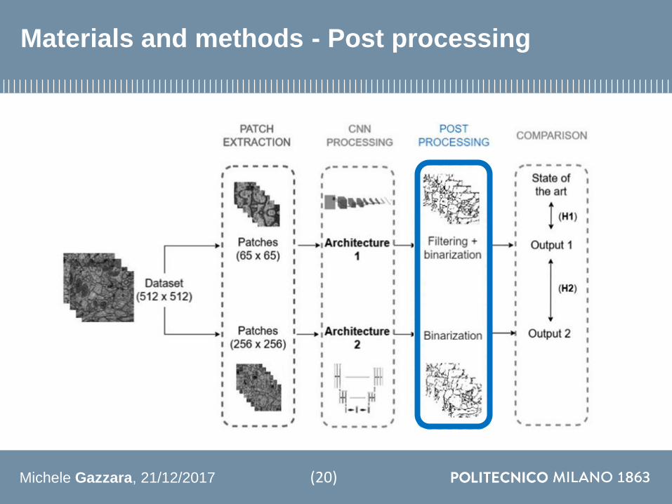
Michele Gazzara 21122017
Materials and methods - Post processing
(20)
Michele Gazzara 21122017
Post processing
Architecture 1
Pixel probability
Spatial imagereconstruction
Medianfiltering
Otsuthresholding
(21)
Michele Gazzara 21122017
Post processing
Architecture 1
Pixel probability
Spatial imagereconstruction
Medianfiltering
Otsuthresholding
(21)
Patch probability
map
Otsuthresholding
Architecture 2
Michele Gazzara 21122017
Materials and methods - Comparison
(22)
Michele Gazzara 21122017
Evaluation protocol - Metrics
Accuracy (Acc)
Pixel error (PE)
Sensitivity (Sn) and Specificity (Sp)
SoslashrensenndashDice coefficient (DSC)
Sn = TP
TP+FN
PE = 1 - Acc
119860119888119888 =1
Nσj=1N 119904119888119900119903119890119895 score = ൝
1 119894119891 yj= ොy1198950 119894119891 yj ne ොy119895
119863119878119862 =2 119879119875
119865119875 + 119865119873 + 2 119879119875
Sp = TN
TN+FP
Where
119962119946 sample label
ෝ119962119946 prediction
N number of samples
i semple index
TP true positives
FN false negatives
TN true negatives
FP false positives
(23)
[I Arganda-Carreras et al 2015]
Michele Gazzara 21122017
Evaluation protocol - H1 and H2
Investigation of H1
VSNon CNN-based approaches
CNN-based approaches
Architecture 1(PE)
(24)
Investigation of H2
Architecture 1(Performance metrics and
computational costs)
Architecture 2(Performance metrics and
computational costs)
VS(Lilliefors and Wilcoxon test)
Michele Gazzara 21122017
Results - Investigation of H1
Model Method PE [∙10minus3]
Architecture 1 CNN 88
Kaynig et al (2010) RF 157
Liu et al (2012) ANN 134
Model Training images Training time PE [∙10minus3]
Architecture 1 327680 5 hours 10 min 88
Ciresan et al (2012) 3 millions 85 hours 60
Fakhry et al (2015) 42 millions 30 hours 51
Comparison with non-CNN based models
Comparison with other CNN based models
(25)
PE = 1 - Acc
Michele Gazzara 21122017
Evaluation protocol - H1 and H2
Investigation of H1
VSNon CNN-based approaches
CNN-based approaches
Architecture 1(PE)
Investigation of H2
Architecture 1(Performance metrics and
computational costs)
Architecture 2(Performance metrics and
computational costs)
VS(Lilliefors and Wilcoxon test)
Michele Gazzara 21122017
Results - Investigation of H2 metrics
(26)
Michele Gazzara 21122017
Results - Investigation of H2 computational costs
(27)
Michele Gazzara 21122017
Results - Segmented images
Architecture 2 output
Architecture 1 output
Input image Ground truth
(28)
Michele Gazzara 21122017
Discussion
H1
1 Architecture 1 performances exceed the non CNN-based models
2 Architecture 1 performances are comparable with other CNN-based models
Reduced dataset and training time
(29)
Michele Gazzara 21122017
Discussion
H1
1 Architecture 1 performances exceed the non CNN-based models
2 Architecture 1 performances are comparable with other CNN-based models
Reduced dataset and training time
H2
1 Architecture 2 overcomes Architecture 1in terms of accuracy
2 Architecture 2 computational costs are lower than Architecture 1
Architecture 1detects more FPs
Architecture 2 can be used for real
time applications
(29)
Michele Gazzara 21122017
Conclusions and future work
CONCLUSIONS
Automatic method for axon segmentation in EM images
Performances comparable with existing CNN models
Reduced computational costs
(30)
Michele Gazzara 21122017
Conclusions and future work
CONCLUSIONS
Automatic method for axon segmentation in EM images
Performances comparable with existing CNN models
Reduced computational costs
FUTURE WORK
Larger dataset
Human brain EM images
Up-convolution improvement
(30)
[H Gao et al 2017]
Michele Gazzara 21122017
Acknowledgements
(31)
Michele Gazzara 21122017
Thank you for your attention
(32)
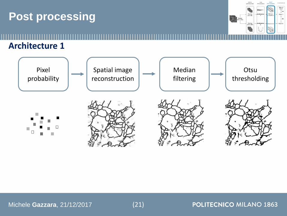
Michele Gazzara 21122017
Post processing
Architecture 1
Pixel probability
Spatial imagereconstruction
Medianfiltering
Otsuthresholding
(21)
Michele Gazzara 21122017
Post processing
Architecture 1
Pixel probability
Spatial imagereconstruction
Medianfiltering
Otsuthresholding
(21)
Patch probability
map
Otsuthresholding
Architecture 2
Michele Gazzara 21122017
Materials and methods - Comparison
(22)
Michele Gazzara 21122017
Evaluation protocol - Metrics
Accuracy (Acc)
Pixel error (PE)
Sensitivity (Sn) and Specificity (Sp)
SoslashrensenndashDice coefficient (DSC)
Sn = TP
TP+FN
PE = 1 - Acc
119860119888119888 =1
Nσj=1N 119904119888119900119903119890119895 score = ൝
1 119894119891 yj= ොy1198950 119894119891 yj ne ොy119895
119863119878119862 =2 119879119875
119865119875 + 119865119873 + 2 119879119875
Sp = TN
TN+FP
Where
119962119946 sample label
ෝ119962119946 prediction
N number of samples
i semple index
TP true positives
FN false negatives
TN true negatives
FP false positives
(23)
[I Arganda-Carreras et al 2015]
Michele Gazzara 21122017
Evaluation protocol - H1 and H2
Investigation of H1
VSNon CNN-based approaches
CNN-based approaches
Architecture 1(PE)
(24)
Investigation of H2
Architecture 1(Performance metrics and
computational costs)
Architecture 2(Performance metrics and
computational costs)
VS(Lilliefors and Wilcoxon test)
Michele Gazzara 21122017
Results - Investigation of H1
Model Method PE [∙10minus3]
Architecture 1 CNN 88
Kaynig et al (2010) RF 157
Liu et al (2012) ANN 134
Model Training images Training time PE [∙10minus3]
Architecture 1 327680 5 hours 10 min 88
Ciresan et al (2012) 3 millions 85 hours 60
Fakhry et al (2015) 42 millions 30 hours 51
Comparison with non-CNN based models
Comparison with other CNN based models
(25)
PE = 1 - Acc
Michele Gazzara 21122017
Evaluation protocol - H1 and H2
Investigation of H1
VSNon CNN-based approaches
CNN-based approaches
Architecture 1(PE)
Investigation of H2
Architecture 1(Performance metrics and
computational costs)
Architecture 2(Performance metrics and
computational costs)
VS(Lilliefors and Wilcoxon test)
Michele Gazzara 21122017
Results - Investigation of H2 metrics
(26)
Michele Gazzara 21122017
Results - Investigation of H2 computational costs
(27)
Michele Gazzara 21122017
Results - Segmented images
Architecture 2 output
Architecture 1 output
Input image Ground truth
(28)
Michele Gazzara 21122017
Discussion
H1
1 Architecture 1 performances exceed the non CNN-based models
2 Architecture 1 performances are comparable with other CNN-based models
Reduced dataset and training time
(29)
Michele Gazzara 21122017
Discussion
H1
1 Architecture 1 performances exceed the non CNN-based models
2 Architecture 1 performances are comparable with other CNN-based models
Reduced dataset and training time
H2
1 Architecture 2 overcomes Architecture 1in terms of accuracy
2 Architecture 2 computational costs are lower than Architecture 1
Architecture 1detects more FPs
Architecture 2 can be used for real
time applications
(29)
Michele Gazzara 21122017
Conclusions and future work
CONCLUSIONS
Automatic method for axon segmentation in EM images
Performances comparable with existing CNN models
Reduced computational costs
(30)
Michele Gazzara 21122017
Conclusions and future work
CONCLUSIONS
Automatic method for axon segmentation in EM images
Performances comparable with existing CNN models
Reduced computational costs
FUTURE WORK
Larger dataset
Human brain EM images
Up-convolution improvement
(30)
[H Gao et al 2017]
Michele Gazzara 21122017
Acknowledgements
(31)
Michele Gazzara 21122017
Thank you for your attention
(32)
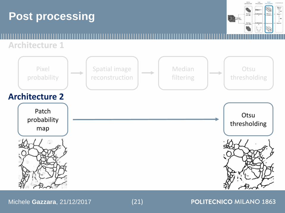
Michele Gazzara 21122017
Post processing
Architecture 1
Pixel probability
Spatial imagereconstruction
Medianfiltering
Otsuthresholding
(21)
Patch probability
map
Otsuthresholding
Architecture 2
Michele Gazzara 21122017
Materials and methods - Comparison
(22)
Michele Gazzara 21122017
Evaluation protocol - Metrics
Accuracy (Acc)
Pixel error (PE)
Sensitivity (Sn) and Specificity (Sp)
SoslashrensenndashDice coefficient (DSC)
Sn = TP
TP+FN
PE = 1 - Acc
119860119888119888 =1
Nσj=1N 119904119888119900119903119890119895 score = ൝
1 119894119891 yj= ොy1198950 119894119891 yj ne ොy119895
119863119878119862 =2 119879119875
119865119875 + 119865119873 + 2 119879119875
Sp = TN
TN+FP
Where
119962119946 sample label
ෝ119962119946 prediction
N number of samples
i semple index
TP true positives
FN false negatives
TN true negatives
FP false positives
(23)
[I Arganda-Carreras et al 2015]
Michele Gazzara 21122017
Evaluation protocol - H1 and H2
Investigation of H1
VSNon CNN-based approaches
CNN-based approaches
Architecture 1(PE)
(24)
Investigation of H2
Architecture 1(Performance metrics and
computational costs)
Architecture 2(Performance metrics and
computational costs)
VS(Lilliefors and Wilcoxon test)
Michele Gazzara 21122017
Results - Investigation of H1
Model Method PE [∙10minus3]
Architecture 1 CNN 88
Kaynig et al (2010) RF 157
Liu et al (2012) ANN 134
Model Training images Training time PE [∙10minus3]
Architecture 1 327680 5 hours 10 min 88
Ciresan et al (2012) 3 millions 85 hours 60
Fakhry et al (2015) 42 millions 30 hours 51
Comparison with non-CNN based models
Comparison with other CNN based models
(25)
PE = 1 - Acc
Michele Gazzara 21122017
Evaluation protocol - H1 and H2
Investigation of H1
VSNon CNN-based approaches
CNN-based approaches
Architecture 1(PE)
Investigation of H2
Architecture 1(Performance metrics and
computational costs)
Architecture 2(Performance metrics and
computational costs)
VS(Lilliefors and Wilcoxon test)
Michele Gazzara 21122017
Results - Investigation of H2 metrics
(26)
Michele Gazzara 21122017
Results - Investigation of H2 computational costs
(27)
Michele Gazzara 21122017
Results - Segmented images
Architecture 2 output
Architecture 1 output
Input image Ground truth
(28)
Michele Gazzara 21122017
Discussion
H1
1 Architecture 1 performances exceed the non CNN-based models
2 Architecture 1 performances are comparable with other CNN-based models
Reduced dataset and training time
(29)
Michele Gazzara 21122017
Discussion
H1
1 Architecture 1 performances exceed the non CNN-based models
2 Architecture 1 performances are comparable with other CNN-based models
Reduced dataset and training time
H2
1 Architecture 2 overcomes Architecture 1in terms of accuracy
2 Architecture 2 computational costs are lower than Architecture 1
Architecture 1detects more FPs
Architecture 2 can be used for real
time applications
(29)
Michele Gazzara 21122017
Conclusions and future work
CONCLUSIONS
Automatic method for axon segmentation in EM images
Performances comparable with existing CNN models
Reduced computational costs
(30)
Michele Gazzara 21122017
Conclusions and future work
CONCLUSIONS
Automatic method for axon segmentation in EM images
Performances comparable with existing CNN models
Reduced computational costs
FUTURE WORK
Larger dataset
Human brain EM images
Up-convolution improvement
(30)
[H Gao et al 2017]
Michele Gazzara 21122017
Acknowledgements
(31)
Michele Gazzara 21122017
Thank you for your attention
(32)

Michele Gazzara 21122017
Materials and methods - Comparison
(22)
Michele Gazzara 21122017
Evaluation protocol - Metrics
Accuracy (Acc)
Pixel error (PE)
Sensitivity (Sn) and Specificity (Sp)
SoslashrensenndashDice coefficient (DSC)
Sn = TP
TP+FN
PE = 1 - Acc
119860119888119888 =1
Nσj=1N 119904119888119900119903119890119895 score = ൝
1 119894119891 yj= ොy1198950 119894119891 yj ne ොy119895
119863119878119862 =2 119879119875
119865119875 + 119865119873 + 2 119879119875
Sp = TN
TN+FP
Where
119962119946 sample label
ෝ119962119946 prediction
N number of samples
i semple index
TP true positives
FN false negatives
TN true negatives
FP false positives
(23)
[I Arganda-Carreras et al 2015]
Michele Gazzara 21122017
Evaluation protocol - H1 and H2
Investigation of H1
VSNon CNN-based approaches
CNN-based approaches
Architecture 1(PE)
(24)
Investigation of H2
Architecture 1(Performance metrics and
computational costs)
Architecture 2(Performance metrics and
computational costs)
VS(Lilliefors and Wilcoxon test)
Michele Gazzara 21122017
Results - Investigation of H1
Model Method PE [∙10minus3]
Architecture 1 CNN 88
Kaynig et al (2010) RF 157
Liu et al (2012) ANN 134
Model Training images Training time PE [∙10minus3]
Architecture 1 327680 5 hours 10 min 88
Ciresan et al (2012) 3 millions 85 hours 60
Fakhry et al (2015) 42 millions 30 hours 51
Comparison with non-CNN based models
Comparison with other CNN based models
(25)
PE = 1 - Acc
Michele Gazzara 21122017
Evaluation protocol - H1 and H2
Investigation of H1
VSNon CNN-based approaches
CNN-based approaches
Architecture 1(PE)
Investigation of H2
Architecture 1(Performance metrics and
computational costs)
Architecture 2(Performance metrics and
computational costs)
VS(Lilliefors and Wilcoxon test)
Michele Gazzara 21122017
Results - Investigation of H2 metrics
(26)
Michele Gazzara 21122017
Results - Investigation of H2 computational costs
(27)
Michele Gazzara 21122017
Results - Segmented images
Architecture 2 output
Architecture 1 output
Input image Ground truth
(28)
Michele Gazzara 21122017
Discussion
H1
1 Architecture 1 performances exceed the non CNN-based models
2 Architecture 1 performances are comparable with other CNN-based models
Reduced dataset and training time
(29)
Michele Gazzara 21122017
Discussion
H1
1 Architecture 1 performances exceed the non CNN-based models
2 Architecture 1 performances are comparable with other CNN-based models
Reduced dataset and training time
H2
1 Architecture 2 overcomes Architecture 1in terms of accuracy
2 Architecture 2 computational costs are lower than Architecture 1
Architecture 1detects more FPs
Architecture 2 can be used for real
time applications
(29)
Michele Gazzara 21122017
Conclusions and future work
CONCLUSIONS
Automatic method for axon segmentation in EM images
Performances comparable with existing CNN models
Reduced computational costs
(30)
Michele Gazzara 21122017
Conclusions and future work
CONCLUSIONS
Automatic method for axon segmentation in EM images
Performances comparable with existing CNN models
Reduced computational costs
FUTURE WORK
Larger dataset
Human brain EM images
Up-convolution improvement
(30)
[H Gao et al 2017]
Michele Gazzara 21122017
Acknowledgements
(31)
Michele Gazzara 21122017
Thank you for your attention
(32)
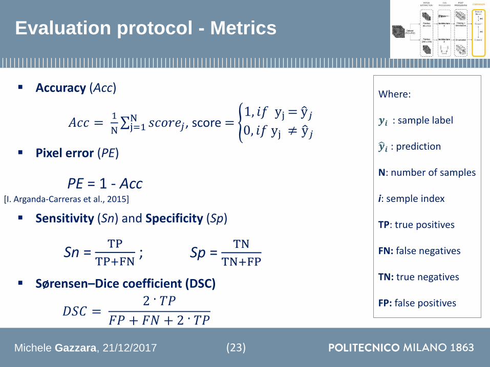
Michele Gazzara 21122017
Evaluation protocol - Metrics
Accuracy (Acc)
Pixel error (PE)
Sensitivity (Sn) and Specificity (Sp)
SoslashrensenndashDice coefficient (DSC)
Sn = TP
TP+FN
PE = 1 - Acc
119860119888119888 =1
Nσj=1N 119904119888119900119903119890119895 score = ൝
1 119894119891 yj= ොy1198950 119894119891 yj ne ොy119895
119863119878119862 =2 119879119875
119865119875 + 119865119873 + 2 119879119875
Sp = TN
TN+FP
Where
119962119946 sample label
ෝ119962119946 prediction
N number of samples
i semple index
TP true positives
FN false negatives
TN true negatives
FP false positives
(23)
[I Arganda-Carreras et al 2015]
Michele Gazzara 21122017
Evaluation protocol - H1 and H2
Investigation of H1
VSNon CNN-based approaches
CNN-based approaches
Architecture 1(PE)
(24)
Investigation of H2
Architecture 1(Performance metrics and
computational costs)
Architecture 2(Performance metrics and
computational costs)
VS(Lilliefors and Wilcoxon test)
Michele Gazzara 21122017
Results - Investigation of H1
Model Method PE [∙10minus3]
Architecture 1 CNN 88
Kaynig et al (2010) RF 157
Liu et al (2012) ANN 134
Model Training images Training time PE [∙10minus3]
Architecture 1 327680 5 hours 10 min 88
Ciresan et al (2012) 3 millions 85 hours 60
Fakhry et al (2015) 42 millions 30 hours 51
Comparison with non-CNN based models
Comparison with other CNN based models
(25)
PE = 1 - Acc
Michele Gazzara 21122017
Evaluation protocol - H1 and H2
Investigation of H1
VSNon CNN-based approaches
CNN-based approaches
Architecture 1(PE)
Investigation of H2
Architecture 1(Performance metrics and
computational costs)
Architecture 2(Performance metrics and
computational costs)
VS(Lilliefors and Wilcoxon test)
Michele Gazzara 21122017
Results - Investigation of H2 metrics
(26)
Michele Gazzara 21122017
Results - Investigation of H2 computational costs
(27)
Michele Gazzara 21122017
Results - Segmented images
Architecture 2 output
Architecture 1 output
Input image Ground truth
(28)
Michele Gazzara 21122017
Discussion
H1
1 Architecture 1 performances exceed the non CNN-based models
2 Architecture 1 performances are comparable with other CNN-based models
Reduced dataset and training time
(29)
Michele Gazzara 21122017
Discussion
H1
1 Architecture 1 performances exceed the non CNN-based models
2 Architecture 1 performances are comparable with other CNN-based models
Reduced dataset and training time
H2
1 Architecture 2 overcomes Architecture 1in terms of accuracy
2 Architecture 2 computational costs are lower than Architecture 1
Architecture 1detects more FPs
Architecture 2 can be used for real
time applications
(29)
Michele Gazzara 21122017
Conclusions and future work
CONCLUSIONS
Automatic method for axon segmentation in EM images
Performances comparable with existing CNN models
Reduced computational costs
(30)
Michele Gazzara 21122017
Conclusions and future work
CONCLUSIONS
Automatic method for axon segmentation in EM images
Performances comparable with existing CNN models
Reduced computational costs
FUTURE WORK
Larger dataset
Human brain EM images
Up-convolution improvement
(30)
[H Gao et al 2017]
Michele Gazzara 21122017
Acknowledgements
(31)
Michele Gazzara 21122017
Thank you for your attention
(32)
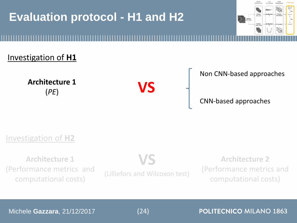
Michele Gazzara 21122017
Evaluation protocol - H1 and H2
Investigation of H1
VSNon CNN-based approaches
CNN-based approaches
Architecture 1(PE)
(24)
Investigation of H2
Architecture 1(Performance metrics and
computational costs)
Architecture 2(Performance metrics and
computational costs)
VS(Lilliefors and Wilcoxon test)
Michele Gazzara 21122017
Results - Investigation of H1
Model Method PE [∙10minus3]
Architecture 1 CNN 88
Kaynig et al (2010) RF 157
Liu et al (2012) ANN 134
Model Training images Training time PE [∙10minus3]
Architecture 1 327680 5 hours 10 min 88
Ciresan et al (2012) 3 millions 85 hours 60
Fakhry et al (2015) 42 millions 30 hours 51
Comparison with non-CNN based models
Comparison with other CNN based models
(25)
PE = 1 - Acc
Michele Gazzara 21122017
Evaluation protocol - H1 and H2
Investigation of H1
VSNon CNN-based approaches
CNN-based approaches
Architecture 1(PE)
Investigation of H2
Architecture 1(Performance metrics and
computational costs)
Architecture 2(Performance metrics and
computational costs)
VS(Lilliefors and Wilcoxon test)
Michele Gazzara 21122017
Results - Investigation of H2 metrics
(26)
Michele Gazzara 21122017
Results - Investigation of H2 computational costs
(27)
Michele Gazzara 21122017
Results - Segmented images
Architecture 2 output
Architecture 1 output
Input image Ground truth
(28)
Michele Gazzara 21122017
Discussion
H1
1 Architecture 1 performances exceed the non CNN-based models
2 Architecture 1 performances are comparable with other CNN-based models
Reduced dataset and training time
(29)
Michele Gazzara 21122017
Discussion
H1
1 Architecture 1 performances exceed the non CNN-based models
2 Architecture 1 performances are comparable with other CNN-based models
Reduced dataset and training time
H2
1 Architecture 2 overcomes Architecture 1in terms of accuracy
2 Architecture 2 computational costs are lower than Architecture 1
Architecture 1detects more FPs
Architecture 2 can be used for real
time applications
(29)
Michele Gazzara 21122017
Conclusions and future work
CONCLUSIONS
Automatic method for axon segmentation in EM images
Performances comparable with existing CNN models
Reduced computational costs
(30)
Michele Gazzara 21122017
Conclusions and future work
CONCLUSIONS
Automatic method for axon segmentation in EM images
Performances comparable with existing CNN models
Reduced computational costs
FUTURE WORK
Larger dataset
Human brain EM images
Up-convolution improvement
(30)
[H Gao et al 2017]
Michele Gazzara 21122017
Acknowledgements
(31)
Michele Gazzara 21122017
Thank you for your attention
(32)

Michele Gazzara 21122017
Evaluation protocol - H1 and H2
Investigation of H1
VSNon CNN-based approaches
CNN-based approaches
Architecture 1(PE)
Investigation of H2
Architecture 1(Performance metrics and
computational costs)
Architecture 2(Performance metrics and
computational costs)
VS(Lilliefors and Wilcoxon test)
Michele Gazzara 21122017
Results - Investigation of H2 metrics
(26)
Michele Gazzara 21122017
Results - Investigation of H2 computational costs
(27)
Michele Gazzara 21122017
Results - Segmented images
Architecture 2 output
Architecture 1 output
Input image Ground truth
(28)
Michele Gazzara 21122017
Discussion
H1
1 Architecture 1 performances exceed the non CNN-based models
2 Architecture 1 performances are comparable with other CNN-based models
Reduced dataset and training time
(29)
Michele Gazzara 21122017
Discussion
H1
1 Architecture 1 performances exceed the non CNN-based models
2 Architecture 1 performances are comparable with other CNN-based models
Reduced dataset and training time
H2
1 Architecture 2 overcomes Architecture 1in terms of accuracy
2 Architecture 2 computational costs are lower than Architecture 1
Architecture 1detects more FPs
Architecture 2 can be used for real
time applications
(29)
Michele Gazzara 21122017
Conclusions and future work
CONCLUSIONS
Automatic method for axon segmentation in EM images
Performances comparable with existing CNN models
Reduced computational costs
(30)
Michele Gazzara 21122017
Conclusions and future work
CONCLUSIONS
Automatic method for axon segmentation in EM images
Performances comparable with existing CNN models
Reduced computational costs
FUTURE WORK
Larger dataset
Human brain EM images
Up-convolution improvement
(30)
[H Gao et al 2017]
Michele Gazzara 21122017
Acknowledgements
(31)
Michele Gazzara 21122017
Thank you for your attention
(32)
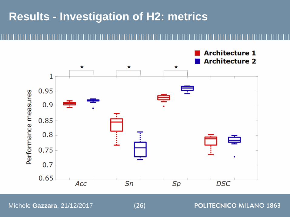
Michele Gazzara 21122017
Results - Segmented images
Architecture 2 output
Architecture 1 output
Input image Ground truth
(28)
Michele Gazzara 21122017
Discussion
H1
1 Architecture 1 performances exceed the non CNN-based models
2 Architecture 1 performances are comparable with other CNN-based models
Reduced dataset and training time
(29)
Michele Gazzara 21122017
Discussion
H1
1 Architecture 1 performances exceed the non CNN-based models
2 Architecture 1 performances are comparable with other CNN-based models
Reduced dataset and training time
H2
1 Architecture 2 overcomes Architecture 1in terms of accuracy
2 Architecture 2 computational costs are lower than Architecture 1
Architecture 1detects more FPs
Architecture 2 can be used for real
time applications
(29)
Michele Gazzara 21122017
Conclusions and future work
CONCLUSIONS
Automatic method for axon segmentation in EM images
Performances comparable with existing CNN models
Reduced computational costs
(30)
Michele Gazzara 21122017
Conclusions and future work
CONCLUSIONS
Automatic method for axon segmentation in EM images
Performances comparable with existing CNN models
Reduced computational costs
FUTURE WORK
Larger dataset
Human brain EM images
Up-convolution improvement
(30)
[H Gao et al 2017]
Michele Gazzara 21122017
Acknowledgements
(31)
Michele Gazzara 21122017
Thank you for your attention
(32)
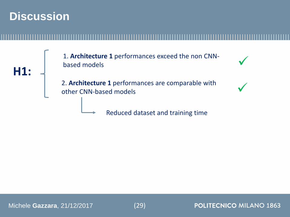
Michele Gazzara 21122017
Discussion
H1
1 Architecture 1 performances exceed the non CNN-based models
2 Architecture 1 performances are comparable with other CNN-based models
Reduced dataset and training time
(29)
Michele Gazzara 21122017
Discussion
H1
1 Architecture 1 performances exceed the non CNN-based models
2 Architecture 1 performances are comparable with other CNN-based models
Reduced dataset and training time
H2
1 Architecture 2 overcomes Architecture 1in terms of accuracy
2 Architecture 2 computational costs are lower than Architecture 1
Architecture 1detects more FPs
Architecture 2 can be used for real
time applications
(29)
Michele Gazzara 21122017
Conclusions and future work
CONCLUSIONS
Automatic method for axon segmentation in EM images
Performances comparable with existing CNN models
Reduced computational costs
(30)
Michele Gazzara 21122017
Conclusions and future work
CONCLUSIONS
Automatic method for axon segmentation in EM images
Performances comparable with existing CNN models
Reduced computational costs
FUTURE WORK
Larger dataset
Human brain EM images
Up-convolution improvement
(30)
[H Gao et al 2017]
Michele Gazzara 21122017
Acknowledgements
(31)
Michele Gazzara 21122017
Thank you for your attention
(32)

Michele Gazzara 21122017
Discussion
H1
1 Architecture 1 performances exceed the non CNN-based models
2 Architecture 1 performances are comparable with other CNN-based models
Reduced dataset and training time
H2
1 Architecture 2 overcomes Architecture 1in terms of accuracy
2 Architecture 2 computational costs are lower than Architecture 1
Architecture 1detects more FPs
Architecture 2 can be used for real
time applications
(29)
Michele Gazzara 21122017
Conclusions and future work
CONCLUSIONS
Automatic method for axon segmentation in EM images
Performances comparable with existing CNN models
Reduced computational costs
(30)
Michele Gazzara 21122017
Conclusions and future work
CONCLUSIONS
Automatic method for axon segmentation in EM images
Performances comparable with existing CNN models
Reduced computational costs
FUTURE WORK
Larger dataset
Human brain EM images
Up-convolution improvement
(30)
[H Gao et al 2017]
Michele Gazzara 21122017
Acknowledgements
(31)
Michele Gazzara 21122017
Thank you for your attention
(32)

Michele Gazzara 21122017
Conclusions and future work
CONCLUSIONS
Automatic method for axon segmentation in EM images
Performances comparable with existing CNN models
Reduced computational costs
(30)
Michele Gazzara 21122017
Conclusions and future work
CONCLUSIONS
Automatic method for axon segmentation in EM images
Performances comparable with existing CNN models
Reduced computational costs
FUTURE WORK
Larger dataset
Human brain EM images
Up-convolution improvement
(30)
[H Gao et al 2017]
Michele Gazzara 21122017
Acknowledgements
(31)
Michele Gazzara 21122017
Thank you for your attention
(32)

Michele Gazzara 21122017
Conclusions and future work
CONCLUSIONS
Automatic method for axon segmentation in EM images
Performances comparable with existing CNN models
Reduced computational costs
FUTURE WORK
Larger dataset
Human brain EM images
Up-convolution improvement
(30)
[H Gao et al 2017]
Michele Gazzara 21122017
Acknowledgements
(31)
Michele Gazzara 21122017
Thank you for your attention
(32)

Michele Gazzara 21122017
Acknowledgements
(31)
Michele Gazzara 21122017
Thank you for your attention
(32)

Michele Gazzara 21122017
Thank you for your attention
(32)