Interpolation over Light Fieldswith Applications in Computer Graphics∗

F. Betul Atalay† David M. Mount‡

Abstract

We present a data structure, called aray interpolant tree, or RI-tree, which stores a discrete set ofdirected lines in 3-space, each represented as a point in 4-space. Each directed line is associated withsome small number of continuous geometric attributes. We show how this data structure can be used foransweringinterpolation queries, in which we are given an arbitrary ray in 3-space and wish to interpolatethe attributes of neighboring rays in the data structure. We illustrate the practical value of the RI-treein two applications from computer graphics: ray tracing and volume visualization. In particular, givenobjects defined by smooth curved surfaces, the RI-tree can produce high-quality renderings significantlyfaster than standard methods. We also investigate a number of tradeoffs between the space and time usedby the data structure and the accuracy of the interpolation results.

1 Introduction

There is a growing interest in algorithms and data structures that combine elements of discrete algorithmdesign with continuous mathematics. This is particularly true in computer graphics. Consider for examplethe process of generating a photo-realistic image. The most popular method for doing this isray-tracing[18]. Ray-tracing models the light emitted from light sources as traveling along rays in 3-space. The color ofa pixel in the image is a reconstruction of the intensity of light traveling along various rays that are emittedfrom a light source, transmitted and reflected among the objects in the scene, and eventually entering theviewer’s eye.

There are many different methods for mapping this approach into an algorithm. At an abstract level, allray-tracers involve forming an image by combining various continuous quantities, orattributes, that havebeen generated from a discrete set of sampled rays. These continuous attributes include color, radiance,surface normals, and reflection and refraction vectors. These attributes vary continuously either as a functionof the location on the surface of an object or as a function of the location of the viewer and the locationsof the various light sources in 3-space. The reconstruction process involves combining various discretelysampled attributes in the context of some illumination model.

Producing images by ray-tracing is a computationally intensive process. The degree of realism in thefinal image depends on a number of factors, including the density and number of samples that are used to

∗A preliminary version of this paper appeared in theProc. of the 5th Workshop on Algorithm Engineering and Experiments(ALENEX 2003), R. Ladner, Editor, SIAM, 2003, 56–68. This material is based upon work supported by the National ScienceFoundation under Grant No. 0098151.

†Department of Computer Science, University of Maryland, College Park, Maryland. Email: betul@cs.umd.edu.‡Department of Computer Science and Institute for Advanced Computer Studies, University of Maryland, College Park, Mary-

land. Email: mount@cs.umd.edu.

1

compute a pixel’s intensity and the fidelity of the illumination model to the physics of illumination. Scenescan involve hundreds of light sources and from thousands to millions of objects, often represented as smoothsurfaces, including implicit surfaces [9], subdivision surfaces [30], and Bezier surfaces and NURBS [14].Reflective and transparent objects cause rays to be reflected and refracted, further increasing the numbersof rays that need to be traced. In traditional ray-tracing solutions, each ray is traced through the scene asneeded to compute the intensity of a pixel in the image [18]. To achieve smoothness avoid problems withaliasing, many rays may be shot for each pixel. A high resolution rendering can easily involve shooting onthe order of hundreds of millions of rays. Much of the computational effort involves determining the firstobject that is intersected by each ray and the location that the ray hits.

In this paper, we propose an approach to help to accelerate this process by reducing the number of inter-section calculations. Our algorithm facilitates fast, approximate rendering of a scene from any viewpoint,and is also useful when the scene is rendered from multiple viewpoints, as arises, for example, in computinganimations. Rather than tracing each input ray to compute the required attributes, we collect and store a rela-tively sparse set ofsampled raysand associate a number of continuous geometric attributes with each samplein a fast data structure. We can then use inexpensiveinterpolationmethods to approximate the value of thesesampled quantities for other input rays. Using an adaptive strategy, it is possible to avoid oversampling insmooth areas while providing sufficiently dense sampling in regions of high variation. We dynamicallymaintain acacheof the most recently generated samples, in order to reduce the space requirements of thedata structure.

The information associated with a given ray is indexed according to the directed line that supports theray, which in turn is modeled as a point in a 4-dimensionalline space. Given a ray to be traced, we accessthe data structure to locate a number of neighboring sampled rays in line space. We then interpolate thecontinuous attributes from the neighboring rays. The resulting data structure is called anray interpolanttree, or RI-treefor short.

1.1 Related Work

The idea of associating radiance information with points in line space has a considerable history, datingback to work in the 1930’s by Gershun on vector irradiance fields [16] and Moon and Spencer’s conceptof photic fields [25], and more recent papers by Levoy and Hanrahan [23] and Gortler, et al. [19]. Theterm “light field” in our title was coined by Levoy and Hanrahan, but our notion is more general than theirsbecause we consider interpolation of any continuous attributes, not just radiance. Most methods for storinglight field information in computer graphics are based on discretizing the space into uniform grids. Incontrast, we sample rays adaptively, concentrating more samples in regions where the variations in attributevalues are higher. The most closely related work to ours is the Interpolant Ray-tracer system introducedby Bala, Dorsey, and Teller [7], which combines adaptive sampling of radiance information, caching, andinterpolation for rendering convex objects. Our method generalizes theirs by storing and interpolating notonly radiance information but other sorts of continuous information, which may be relevant to the renderingprocess. In Section 3.9 we demonstrate the value of this approach. We also allow nonconvex objects. Unliketheir method, however, we do not provide guarantees on the worst-case approximation error.

In addition, there has been earlier research on accelerating ray tracing by reducing the cost of intersectioncomputations using bounding volume hierarchies [22, 27], space partitioning structures [15, 17, 21], andmethods exploiting ray coherence [1, 5, 20, 26]. Many of these methods can be applied in combination withours.

2

The design of efficient data structures for ray-tracing has been of interest in the field of computationalgeometry. This includes, for example, the work of Mitchell, Mount and Suri on simple cover complexity[24], the work of Aronov and Fortune on low weight triangulations [4], cost prediction for ray shooting byAronov, Bronnimann, Chang and Chiang [2, 3] and hierarchical uniform grids (HUG) space partitioningdata structure introduced by Cazals, Drettakis and Puech [10]. In a later study, Cazals and Puech compareduniform grids, recursive grids, and HUG for ray-tracing, and demonstrated statistically that recursive gridsand HUG outperform uniform grids for non-uniform distribution of scene objects[11].

A simpler variant of this data structure was introduced by the authors in [6]. The current data structurehas two main improvements over the previous one. Firstly, the previous data structure was not dynamic. Inthe preprocessing phase, the entire data structure was built sampling millions of rays originating from theentire space of viewpoints in various directions. This resulted in high preprocessing times, and high spacerequirements. The current data structure, on the other hand, is built dynamically. Samples are generatedon demand—only when they are actually needed, and maintained by a caching mechanism. Secondly, thecurrent system generalizes the framework and can handle scenes containing multiple objects with differentsurface reflectance properties, whereas the previous system focused on single reflective or transparent object.In addition, a systematic analysis of the performance of the data structure is presented in this paper.

1.2 Design Issues

The approach of computing a sparse set of sample rays and interpolating the results of ray shooting is mostuseful for rendering smooth objects that are reflective or transparent, for rendering animations when theviewpoint varies smoothly, and for generating high-resolution images and/or antialiased images generatedby supersampling [18] in which multiple rays are shot for each pixel of the image.

Although we have motivated the RI-tree data structure from the perspective of ray-tracing, there area number of applications having to do with lines in 3-space that can benefit from this general approach.To illustrate this, we have studied two different applications, one involving image generation through ray-tracing and the other involving volume visualization with applications in medical imaging for radiationtherapy.

There are a number of issues that arise in engineering a practical data structure for interpolation in linespace. These include the following.

How and where to sample rays?Regions of space where continuous information varies more rapidly needto be sampled with greater density than regions that vary smoothly.

Whether to interpolate? In the neighborhood of a discontinuity, the number of rays that may need to besampled to produce reasonable results may be unacceptably high. Because the human eye is verysensitive to discontinuities near edges and silhouettes, it is often wise to avoid interpolating acrossdiscontinuities. This raises the question of how to detect discontinuities. When they are detected, is itstill possible to interpolate or should we avoid interpolation and use standard ray-tracing instead?

How many samples to maintain?Even for reasonably smooth scenes, the number of sampled rays thatwould need to be stored for an accurate reconstruction runs well into millions. For this reason, wecachethe results of only the most relevant rays. What are the space-time tradeoffs involved with thisapproach?

3

We investigate these and other questions in the context of a number of experiments based on the ap-plications mentioned above. The paper is organized as follows. In the rest of this section, we give a briefoverview of our algorithm in the context of ray-tracing. In Section 2, we explain the construction of our datastructure, and its use for answeringinterpolation queries. In Section 3, we report experimental results.

1.3 Algorithm Overview

In order to make things concrete, we will describe our data structure in terms of a ray-tracing application. Asmentioned in the introduction, ray-tracing works by simulating the light propagation in a scene. A traditionalray-tracer shoots one or more rays from the viewpoint through each pixel of the image plane. Each ray istraced through the scene and the light intensity that is gathered determines the color of the correspondingpixel. To reduce problems of aliasing, multiple rays may also be traced for each pixel and these results areaveraged.

We can distinguish two major tasks in a ray-tracer. Thegeometric componentis responsible for cal-culating the closest visible object point along a specific ray, as theshading componentcomputes the colorof that point. If the object is reflective or transparent, the reflection and transmission rays are traced recur-sively to gather their contribution to the intensity. The primary expense in ray-tracing lies in the geometriccomponent, especially for scenes that contain complex objects such as Bezier or NURBS surfaces, and/orreflective and refractive objects.

Each object can be modeled abstractly as a functionf mapping input rays to a set of geometric attributes,which are used in color and shading computation. The attributes depend on the object’s surface reflectanceproperties. For objects whose surfaces are neither reflective nor transparent, denotedsimple surfaces, thefunction returns the point of intersection and the surface normal at this point. For objects whose surfaces areeither reflective or transparent the function additionally returns theexit ray, that is, the reflected or refractedray, respectively, that leaves the object’s surface. The exit ray is represented by its origin, theexit point,and directionalexit vector. In general, objects that are both reflective and refractive could be handled byassociating multiple exit rays with an input ray, but our implementation currently does not support this.These quantities are depicted in Figure 1 and the function is described schematically below. We will referto the combination of the underlined attributes below as theoutput ray.

For simple surfaces: f : Ray→ {Normal, IntersectionPoint}Otherwise: f : Ray→ {Normal, IntersectionPoint, ExitPoint, ExitVector}

���

���

���

���

������

������ ff

intersection point intersection point exit point

normal

input ray

exit vector

normal

input ray

Simple Object Refractive Object

Figure 1: Geometric attributes.

4

For many real world objects, which have large smooth surfaces,f is expected to vary smoothly. In thecontext of ray-tracing, this is referred to asray coherence. Nearby rays follow similar paths, hit nearbypoints having similar normal vectors and hence are subject to similar reflections and/or refractions. In theneighborhood of discontinuities, however, nearby input rays may follow quite different paths. In cases wherewe cannot find sufficient evidence to interpolate, we perform ray-tracing instead.

In a traditional ray-tracer, each object is associated with a procedure that computes intersections betweenrays and this object. For objects whose boundaries are sufficiently smooth, we replace this intersection pro-cedure with a data structure, which will be introduced in the next section. This data structure approximatesthe functionf through interpolation.

2 The Ray Interpolant Tree

In this section we introduce the main data structure used in our algorithm, theRI-treeor ray interpolant tree.Each RI-tree is associated with a singleobjectof the scene, which is loosely defined to be a collection oflogically related surfaces. The object is enclosed by an axis-aligned bounding box. The data structure storesthe geometric attributes associated with some set of sampled rays, which may originate from any point inspace and intersect the object’s bounding box.

2.1 Parameterizing Rays as Points

We will model each ray by the directed line that contains the ray. Directed lines can be represented as a pointlying on a 4-dimensional manifold in 5-dimensional projective space using Plucker coordinates [29], but wewill adopt a simpler representation, called thetwo-plane parameterization[19, 23, 7]. A directed line is firstclassified into one of 6 different classes (corresponding to 6plane pairs) according to the line’sdominantdirection, defined to be the axis corresponding to the largest coordinate of the line’s directional vector andits sign. (Ties may be broken arbitrarily.) These classes are denoted+X,−X, +Y,−Y,+Z,−Z. The

dw

h

(s,t)

(u,v)

d + 2w

h+ 2

w

Front Plane Back Plane

X

ZY

Figure 2: The two-plane parameterization of directed lines and rays. The +X plane pair is shown.

directed line is then represented by its two intercepts(s, t) and(u, v) with the front planeandback plane,respectively, that are orthogonal to the dominant direction and coinciding with the object’s bounding box.

5

uv

s

t

of left child

of right childfront plane

��������

��������

front plane

Front plane of parent

Back plane

Figure 3: Subdivision along s-axis.

Now, For example, as shown in Figure 2, rayR with dominant direction+X first intersects the front planeof the+X plane pair at(s, t), and then the back plane at(u, v), and hence is parameterized as(s, t, u, v).Note that, the+X and−X involve the same plane pair but differ in the distinction between front and backplane. It is easy to see that if the bounding box has widthw (alongx), heighth (alongy) and depthd (alongz), then a ray that intersects the bounding box and whose dominant direction is±X intersects the front andback planes through two parallel rectangles of heighth + 2w and depthd + 2w. (See Figure 2.)

2.2 The RI-tree

The RI-tree is a binary tree based on a recursive subdivision of the 4-dimensional space of directed lines. Itconsists of six separate 4-dimensional kd-trees [8, 28] one for each of the six dominant directions. The rootof each kd-tree is a 4-dimensional hypercube in line space containing all rays that are associated with thecorresponding plane pair. The 16 corner points of the hypercube represent the 16 rays from each of the fourcorners of the front plane to the each of the four corners of the back plane. Each node in this data structure isassociated with a 4-dimensional hyperrectangle, called acell. The 16 corner points of a leaf cell constitutethe ray samples, which form the basis of our interpolation. When the leaf cell is constructed, these 16 raysare traced and the associated geometric attributes are stored in the leaf.

2.3 Adaptive Subdivision and Cache Structure

The RI-tree grows and shrinks dynamically based on demand. Initially only the root cell is built by samplingits 16 corner rays. A leaf cell is is subdivided by placing a cut-plane at the midpoint orthogonal to the coor-dinate axis with the longest length. In terms of the plane pair, this corresponds to dividing the correspondingfront or back plane through the midpoint of the longer side. We partition the existing 16 corner samplesbetween the two children, and sample eight new corner rays that are shared between the two child cells.(These new rays are illustrated in Figure 3 in the case that thes-axis is split.)

Rays need to be sampled more densely in some regions than others, for example, in regions wheregeometric attributes have greater variation. For this reason, the subdivision is carried out adaptively basedon the distance between output attributes. The distance between two sets of output attributes are definedas the distance between their associated output rays. We define thedistancebetween two rays to be theL2

distance between their 4-dimensional representations. To determine whether a cell should be subdivided,we first compute the correct output ray associated with the midpoint of the cell, and then we compute an

6

approximate output ray by interpolation of the 16 corner rays for the same point. If the distance betweenthese two output rays exceeds a given user-defineddistance thresholdand the depth of the cell in the tree isless than a user-defineddepth constraint, the cell is subdivided. Otherwise the leaf is said to befinal.

If we were to expand all nodes in the tree until they are final, the resulting data structure could be verylarge, depending on the distance threshold and the depth constraint. For this reason we only expand a nodeto a final leaf if this leaf node is needed for some interpolation. Once a final leaf node is used, it is markedwith a time stamp. If the size of the data structure exceeds a user-definedcache size, then the the tree ispruned to a constant fraction of this size by removing all but the most recently used nodes. In this way, theRI-tree behaves much like an LRU-cache.

θr

1

r

Figure 4: Maximum angle isachieved by the cross diagonals oforthogonally opposing faces.

Comment on the depth constraint: An absolute bound on themaximum tree depth is a rather unnatural parameter. It is, however,possible to infer this value based on some more geometrically naturalparameters. For example, consider instead aangular similarity con-straint, θ, which bounds the maximum angle between any two inputrays that fall within the same leaf cell. In other words, if the anglebetween any two input rays that lie within the same leaf cell of thesubdivision is at mostθ, then these samples are sufficiently close toone another that further subdivision is not required.

Let us illustrate how to compute the tree depth constraint fromθ.We assume for simplicity that the object has been enclosed within abounding cube. Since angles are not affected by uniform scaling, wemay assume that this is a unit cube. It follows from our parameteri-zation, that for each of the dominant directions, it suffices to consider rays that intersect a pair of parallelsquares lying on the front and back planes for this direction, whose side lengths are 3 units. (ConsiderFigure 2 in the casew = h = d = 1.) Now, consider any leaf cell of the associated tree for this direction.Such a cell corresponds to the set of rays passing through two rectangular faces, one on each of these twoparallel squares. Since the sides of each rectangle are alternatingly split along the side of maximum length,the worst case arises when both sides of these faces are of equal length, sayr. (See Figure 4.) Among the16 corner rays sampled for any face pair, it can be shown that the maximum angle occurs between the crossdiagonals of two faces that are aligned orthogonally opposite one another, that is, so that the line connectingthe centers of these two faces is orthogonal to both faces. In this case, the diagonals are of equal length andintersect at their midpoints, from which we have

tanθ

2=

r√

2/21/2

= r√

2,

And so,r = (tan(θ/2))/√

2. Since four splits are required to halve the side length of a cell, and the initial(root) face is of side length 3, it follows that the maximum depth constraint, as a function of the angularsimilarity constraint, is

depth(θ) = 4 lg3r

= 4 lg3√

2tan θ

2

= 4 lg(

3√

2 cotθ

2

),

wherelg denotes logarithm base 2.We set a fixed depth constraints in our experiments, but this formulation in terms of an angular similarity

constraint would be a more appropriate parameter for software design purposes.

7

2.4 Rendering and Interpolation Queries

Recall that our goal is to use interpolation between sampled output rays whenever things are sufficientlysmooth. RI-tree can be used to perform a number of functions in rendering, including determining the firstobject that a ray hits, computing the reflection or refraction (exit) ray for nonsimple objects, and answeringvisibility queries, which are used for example to determine whether a point is visible to a light source or ina shadow.

Let us consider the interpolation of a given input rayR. We first mapR to the associated point in the4-dimensional directed line space and, depending on the dominant direction of this line, we find the leaf cellof the appropriate kd-tree through a standard descent. Since the nodes of the tree are constructed only asneeded, it is possible thatR will reside in a leaf that is not marked asfinal. This means that this particularleaf has not completed its recursive subdivision. In this case, the leaf is subdivided recursively, along thepathR would follow, until the termination condition is satisfied, and the final leaf containingR is nowmarked asfinal. (Other leaves generated by this process are not so marked.)

front plane

(s,t)

NE

back plane

R

(u, v)

Figure 5: Sampled rays within a directional group.

Given the final leaf cell containingR, the output attributes forR can now be interpolated. Interpolationproceeds in two steps. First we group the rays in groups of four, which we call thedirectional groups. Raysin the same group originate from the same corner point on the front plane, and pass through each of the fourcorners of the back plane (For example, Figure 5 shows the rays that originate from the north-east corner ofthe front plane). Within each directional group, bilinear interpolation with respect to the(u, v) coordinates isperformed to compute intermediate output attributes. The outputs of these interpolations are then bilinearlyinterpolated with respect to the(s, t) coordinates to get the approximate output attributes forR. Thus, thisis essentially a quadrilinear interpolation.

2.5 Handling Discontinuities and Regions of High Curvature

Through the use of interpolation, we can greatly reduce the number of ray samples that would otherwise beneeded to render a smooth surface. However, if the ray-output functionf contains discontinuities, as mayoccur at the edges and the outer silhouettes of the object, then we will observe bleeding of colors acrossthese edges. This could be remedied by building a deeper tree, which might involve sampling of rays up topixel resolution in the discontinuity regions. This could result in unacceptably high memory requirements.Instead our approach will be to detect and classify discontinuity regions. In some cases we apply a moresophisticated interpolation. Otherwise we do not interpolate and instead simply revert to ray-tracing. Wewill present a brief overview of how discontinuities are handled here. Further details are presented in [6].

Our objects are specified as a collection of smooth surfaces, referred to aspatches. Each patch isassigned apatch-identifier. Associated with each sample ray, we store the patch-identifier of the first patch

8

it hits. Since each ray sample knows which surface element it hits, it is possible to disallow any interpolationbetween different surfaces. It is often the case, however, that large smooth surfaces are composed of manysmaller patches, which are joined together along edges so that first and second partial derivatives varycontinuously across the edge. In such cases interpolation is allowed. We assume that the surfaces of thescene have been provided with this information, by partitioning patches into surface equivalence classes. Ifthe patch-identifiers associated with the 16 corner ray samples of a final leaf are in the same equivalenceclass, we conclude that there is no discontinuities crossing the region surrounded by the 16 ray hits, and weapply the interpolation process described above.

Requiring that all 16 patches arise from the same equivalence class can significantly limit the number ofinstances in which interpolation can be applied. After all, linear interpolation in 4-space can be performedwith as few as 5 sample points. If the patch-identifiers for the 16 corner samples of the leaf arise from morethan two equivalence classes, then we revert to ray tracing. On the other hand, if exactly two equivalenceclasses are present, implying that there is a single discontinuity boundary, then we perform an intersectiontest to determine which patch the query ray hits. Letpr denote this patch. This intersection test is not asexpensive as a general tracing of the ray, since typically only a few patches are involved, and only the firstlevel intersections of a ray-tracing procedure is computed (that is, no reflection rays or light rays need betraced). Among the 16 corner ray samples, only the ones that hit a patch in the same equivalence class aspr areusableas interpolants. These are the ray samples hitting the same side of a discontinuity boundary asthe query ray. If we determine that there is a sufficient number ofusableray samples, we then interpolatethe ray. Otherwise, we use ray-tracing. See [6] for further details.

Even if interpolation is allowed by the above criterion, it is still possible that interpolation may beinappropriate because the surface has high curvature, resulting in very different output rays for nearbyinput rays. High variations in the output ray (i.e. normal or the exit ray), signal a discontinuous region.As a measure to determine the distance between two output rays, we use the angular distance between theirdirectional vectors. If any pairwise distance between the output rays corresponding to the usable interpolantsis greater than a givenangular threshold, then interpolation is not performed.

3 Experimental Results

The data structure described in the previous section is based on a number of parameters, which directlyinfluence the algorithm’s accuracy and the size and depth of the tree, and indirectly influences the runningtime. We have implemented the data structure and have run a number of experiments to test its performanceas a function of a number of these parameters. We have performed our comparisons in the context of twoapplications.

Ray-tracing: This has been described in the previous section. We are given a scene consisting of objectsthat are either simple, reflective or transparent and a number of light sources. The output is a renderingof the scene from one or more viewpoints.

Volume Visualization: This application is motivated from the medical application of modeling the amountof radiation absorbed in human tissue [12]. We wish to visualize the absorption of radiation througha set of nonintersecting objects in 3-space. In the medical application these objects may be models ofhuman organs, bones, and tumors. For visualization purposes, we treat these shapes as though theyare transparent (but do not refract light rays). If we imagine illuminating such a scene by x-rays, then

9

the intensity of a pixel in the image is inversely proportional to the length of its intersection with thevarious objects of the scene. For each object stored as an RI-tree, the geometric attribute associatedwith each ray is this intersection length.

We know of no comparable algorithms or data structures with which to compare our data structure.Existing image-based data structures [19, 23] assume a dense sampling of the light field, which wouldeasily exceed our memory resources at the resolutions we would like to consider. The Interpolant Ray-tracer system by Bala, et al. [7] only deals with convex objects, and only interpolates radiance information.Our data structure can handle nonconvex objects and may interpolate any type of continuous attributes. Inthe ray-tracing application, for example, we prefer interpolating normals (for a simple object), rather thaninterpolating radiance. In Section 3.9, we provide a comparison of radiance versus normal interpolation insuch a case.

3.1 Test Inputs

We have generated a number of input scenes including different types of objects. As mentioned earlier, foreach object in a scene we may choose to represent it in the traditional method or to use our data structure.Our choice of input sets has been influenced by the fact that the RI-tree is most beneficial for high-resolutionrenderings of smooth objects, especially those that are reflective or transparent. We know of no appropriatebenchmark data sets satisfying these requirements, and so we have generated our own data sets.

Bezier Surface: This surface is used to demonstrate the results of interpolation algorithm for smooth re-flective objects. It is a reflective surface consisting of 100 Bezier patches, joined withC2 continuityat the edges. The surface is placed within a large sphere, which has been given a pseudo-randomprocedural texture [13]. Experiments run with the Bezier surface have been averaged over renderingsof the surface from 3 different viewpoints. Figure 13(a) shows the Bezier surface from one viewpoint.We rendered images of size600 × 600 without anitaliasing. (That is, only one ray is shot per pixel.)

Random volumes: We ran another set of experiments on randomly generated refractive, nonintersecting,convex Bezier objects. In order to generate nonintersecting objects, a given region is recursively sub-divided into a given number of non-intersecting cells by randomly generated axis-aligned hyperplanes,and a convex object is generated within each such cell. Each object is generated by first generating arandom convex planar polyline that defines the silhouette of right half of the object. The vertices ofthe polyline constitute the control points for a random number (n) of Bezier curves, ranging from 5to 16. Then a surface of revolution is generated, giving rise to4n Bezier surface patches. The vol-umes are used both for the ray-tracing and the volume visualization experiments. For ray-tracing werendered anti-aliased images of size300 × 300 (with 9 rays shot per pixel). For volume visualizationwe rendered600× 600 images without antialiasing. Results are averaged over three different randomscenes containing 8, 6, and 5 volumes respectively. Figure 14 shows a scene of refractive volumes.

Tomatoes: This is a realistic scene used to demonstrate the performance and quality of our algorithm forreal scenes. The scene consists of a number of tomatoes, modeled as spheres, placed within a reflectivebowl, modeled using Bezier surfaces. This is covered by a reflective and transparent but non-refractiveplastic wrap (the same Bezier surface described above). There is a Bezier surface tomato next to thebowl, and they are both placed on a reflective table within a large sphere. The wrap reflects theprocedurally textured sphere. The scene is shown in Figure 12.

10

0 0.05 0.1 0.15 0.2 0.25

4D Distance Threshold

3

3.25

3.5

3.75

4

4.25

4.5

4.75

5S

peed

-up

( F

LOP

s)

Speed-Up (FLOPs) vs. Distance Threshold

(a)

0 0.05 0.1 0.15 0.2 0.25

4D Distance Threshold

1.75

2

2.25

2.5

Spe

ed-u

p (

CP

U-t

ime)

Speed-Up (CPU-time) vs. Distance Threshold

(b)

0 0.05 0.1 0.15 0.2 0.25

4D Distance Threshold

0

0.0025

0.005

0.0075

0.01

0.0125

0.015

0.0175

0.02

RG

B-E

rror

RGB-Error vs. Distance Threshold

(c)

Figure 6: Varying the distance threshold. (Angular threshold =30◦, maximum tree depth = 28, for a600 ×600 image, without antialiased). Note that they-axis does not always start at 0.

3.2 Metrics

We measured thespeedupandactual errorcommitted as a function of four different parameters. Speedupis defined both in terms of number of floating point operations, orFLOPs, and CPU-time. FLOP speedup isthe ratio of the number of FLOPs performed by traditional ray-tracing to the number of FLOPs used by ouralgorithm to render the same scene. Similarly, CPU speedup is the ratio of CPU-times. Note that FLOPs andCPU-times for our algorithm include both the sampling and interpolation time. FLOP counts are machineindependent, but they tend to underestimate the time spent in data structure access. However, our experiencehas shown that this access time is not a dominant component of the overall running time.

The actual error committed in a ray-tracing application is measured as the averageL2 distance betweenthe RGB values of corresponding pixels in a ray-traced image and the interpolated image. RGB value is a3-dimensional vector with values normalized to the range[0, 1]. Thus the maximum possible error is

√3.

The error in a volume visualization application is measured as the average distance between the actual length

11

attribute and the corresponding interpolated length attribute.

3.3 Varying the Distance Threshold

Recall that the distance threshold, described in Section 2.3, is used to determine whether an approximateoutput ray and the corresponding actual output ray are close enough (in terms ofL2 distance) to terminatea subdivision process. We varied the distance threshold from0.01 to 0.25 while the other parameters arefixed. The results for the Bezier surface scenes are shown in Figure 6.

As expected, the actual error decreases as the threshold is lowered, due to denser sampling. But, theoverhead of more sample computations reduces the speedup. However, even for low thresholds where theimage quality is high, the CPU-speedup is greater than 2 and the FLOP-speedup is greater than 3. Thesespeedups can be quite significant for ray-tracing, where a single frame can take a long time to render.

Figure 13 (b) and (c) demonstrate how the variation in error reflects the changes in the quality of therendered image. Notice the blockiness in part (c) when the data structure is not subdivided as densely as inpart (b).

0 10 20 30

Angular Threshold

2

2.25

2.5

2.75

3

3.25

3.5

3.75

4

Spe

ed-u

p (

FLO

Ps)

Speed-Up (FLOPs) vs. Angular Threshold

(a)

0 10 20 30

Angular Threshold

0

0.0025

0.005

0.0075

0.01

0.0125

0.015

RG

B-E

rror

RGB-Error vs. Angular Threshold

(b)

Figure 7: Varying angular threshold (distance threshold=0.25, maximum depth=28,300× 300, antialiased).

3.4 Varying the Angular Threshold

The angular threshold, described in Section 2.5, is applied to each query to determine whether the surfacecurvature variation is too high to apply interpolation. We investigated the speedup and error as a function ofthe angular threshold over the renderings of three different random volume scenes. The angular threshold isvaried from5◦ to 30◦. The results are shown in Figure 7.

For lower thresholds, fewer rays could be interpolated due to distant interpolants, and those rays aretraced instead. In this case, the actual error committed is smaller but at the expense of lower speedups.However, the speedups are still acceptable even for low thresholds.

12

22 23 24 25 26 27 28 29 30

Tree Depth

3

3.25

3.5

3.75

4S

peed

-up

( F

LOP

s)

Speed-Up (FLOPs) vs. Tree Depth

(a)

22 23 24 25 26 27 28 29 30

Tree Depth

0

0.005

0.01

0.015

0.02

0.025

0.03

RG

B-E

rror

RGB-Error vs. Tree Depth

(b)

Figure 8: Varying tree depth (distance threshold=0.05, angular threshold=30,600 × 600, non-antialiased).

3.5 Varying the Maximum Tree Depth

Recall that the maximum tree depth, described in Section 2.3, is imposed to avoid excessive tree depthnear discontinuity boundaries. We considered maximum depths ranging from 22 to 30—corresponding toangular similarity ranges of11◦ down to2.7◦ (Because this is a kd-tree in 4-space, four levels of descent aregenerally required to halve the the diameter of a cell). The results for the Bezier surface scenes are shownin Figure 8. The angular threshold is fixed at30◦, and the distance threshold is fixed at0.05.

As the tree is allowed to grow up to a higher depth, rays are sampled with increasing density in theregions where the geometric attributes have greater variation, and thus, error committed by the interpolationalgorithm decreases with higher depths. The speedup graph shows a more interesting behavior. Up to acertain depth, the speedup increases with depth. Speedups are poor for very low-depth trees, since manyof the interpolants cannot pass the angular threshold test, and so many rays need to be traced rather thaninterpolated. However, the speedup decreases with very large depth values, since the overhead caused bydenser sampling starts to dominate.

It seems that a wise choice of depth would be a value that results in both a lower error, and reasonablespeedup. For example for the given graph, depth around 28 would be a good choice for this image. (Thiscorresponds to angular similarity constraint of roughly3.8◦.) However, peak performance depends on anumber of parameters that are particular to the ray tracing application, such as the expected cost of a singleray shoot. In addition, Tables 4–6 shows the required memory when depth is varied. When the tree isunnecessarily deep, not only does the speedup decrease, but space requirements increase as well.

3.6 Varying the Cache Size

As mentioned earlier, the RI-tree functions as an LRU cache. If an upper limit for the available memory—the cache size—is specified, the least recently used paths are pruned based on time stamps set whenever apath is accessed. Excessively small cache sizes can result in frequent regeneration of the same cells. Forthe Bezier surface scene, we have varied the cache size from 0.128 to 2.048 megabytes (MB). The resultingspeedup graph is shown in Figure 9.

13

0 0.5 1 1.5 2 2.5 3Cache Size (MB)

11.25

1.5

1.75

22.25

2.5

2.75

33.25

3.5

3.75

4S

peed

-up

( F

LOP

s)

Speed-Up (FLOPs) vs. Cache Size

(a)

0 0.5 1 1.5 2 2.5Cache Size (MB)

0

0.25

0.5

0.75

1

1.25

1.5

1.75

2

2.25

2.5

Spe

ed-u

p (

CP

U-t

ime)

Speed-Up (CPU-time) vs. Cache Size

(b)

Figure 9: Varying cache size (distance threshold = 0.05, angular threshold = 30, maximum tree depth = 28,600 × 600 image, non-antialiased).

Notice that we used small cache sizes to demonstrate the sudden increase in speedup as the cache sizeapproaches a reasonable value. Normally, we set the cache size to 100MB which is high enough to handlebigger scenes with many data structures. There are additional parameters involved in garbage collection,such as what percentage of the cache should be pruned. In these experiments, each garbage collectionprunes 70% of the cache.

3.7 Volume Visualization Experiments

We have tested the algorithm for the volume visualization application using the same random volumes weused for refractive objects. Images are600× 600 and not antialiased. Results of our sample runs are shownin Table 4-6. The FLOP speedup varies from2.817 to 3.549, and CPU speedup varies from2.388 to 2.814.For higher resolutions, or anti-aliased images the speedups could be higher. The error could be as low as0.008 for low distance thresholds, and is still at a reasonable value for higher thresholds. Figure 15 showsthe actual image, and the interpolated image visualizing one of the random volume scenes. All objects have0.5 opacity, and all have solid gray colors.

Dist Thresh Ang Thresh Tree Depth Speedup (FLOP) Speedup (CPU-time) Error Memory (MB)0.25 30 28 2.65 1.89 0.00482 340.05 10 28 2.40 1.75 0.00190 47

Table 1: Sample results for tomatoes scene (1200 × 900 non-antialiased).

3.8 Performance and Error for Tomatoes Scene

Finally, we have tested the algorithm on the tomatoes scene generating an image of size1200 × 900, non-antialiased. Table 1 shows sample results for the tomato scene and Figure 12 shows the corresponding

14

images. Figure 12(a) shows the ray-traced image. Part (b) shows the interpolated image, and a correspondingcolor-coded image in which the white regions denote the pixels that were traced rather than interpolated.Part (c) shows the interpolated image generated with lower thresholds and the corresponding color-codedimage. Notice that the artifacts in part (b) are corrected in part (c).

Note that the closest objects along the eye rays are correctly determined by interpolation, as are thereflection rays from the wrap and the bowl, and the shadows. The sky is reflected on the wrap. As expected,for lower threshold values we can get a very high quality image and still achieve speedups of 2 or higher. Ifquality is not the main objective, we can get approximate images at higher speedups. The error given is theaverage RGB-error as explained above.

3.9 Radiance versus Ray Interpolation

As we have mentioned before, in a ray-tracing application, we prefer interpolating normals (for a simpleobject), rather than interpolating radiance. Consider the Bezier surface scene, where the surface is simple(neither reflective nor refractive), but the specularity is high. Figure 10 shows the ray-traced image1 of apart of the surface illuminated by 2 light sources.

(a) (b)

Figure 10: (a) Ray-traced simple Bezier surface (b) Upper right part zoomed.

The comparison of radiance versus normal interpolation is somewhat analogous to the difference in theinterpolation methods used in Gouraud and Phong shading. If we choose to interpolate radiance, similar toGauraud shading, we may have to collect samples much more densely, in the regions near specular highlightsin order to achieve greater fidelity, since in those regions radiance varies rapidly. However, when we chooseto interpolate normals and then compute shading with respect to the interpolated normal, dense sampling isonly required in areas where the surface is not smooth enough, regardless of the radiance.

Consider Figure 11. In part (a), the leftmost image shows the surface rendered by using RI-tree, wherenormals are interpolated. The maximum depth allowed is 28, and this is enough to obtain a high qualityapproximation to the ray-traced image in Figure 10. The middle image is a visualization of the RI-tree cells.The rightmost image color codes the depth of the leaf cell used to interpolate the associated pixel. The

1For full resolution images visithttp://www.cs.umd.edu/˜mount/Projects/InterpOLF.

15

(a)

(b)

(c)

16 24 3280Leaf Depth

(d)

Figure 11: (a) Normal-interpolation, max. depth = 28, no. of nodes = 7.4K. (b) Normal-interpolation, max.depth =32, no. of nodes = 13K. (c) Radiance interpolation, max. depth = 32, no. of nodes = 25K. (d) Depth-color scale. 16

depth-color scale is given in part (d). Part (b) gives the corresponding images when the depth is allowed togrow up to 32, some cells are refined more around regions of high curvature.

Part (c) shows the images when the image is rendered by radiance interpolation such that the tree isrefined according to the variance in radiance. To generate an image of comparable quality to (a) and (b),the maximum depth should be set to at least 32. (For values lower than 32, the highlights are noticeablydistorted.) Number of nodes are 7.4K, 13K, and 25K for parts (a), (b) and (c) respectively. Note that Part(a) is a high quality approximation to the ray-traced version, and to achieve the same quality by radianceinterpolation, 3 times more nodes should be generated.

3.10 Animations

In an animation sequence, since many samples will be reused by subsequent frames, we expect that theperformance gain after the first frame would be higher. We have tested the algorithm on the following twoanimation sequences. In both cases, the degree of speedup for the first frame was considerably lower thansubsequent frames, since the data structure is built from scratch for the first frame, and subsequent framescan reuse some or all of the existing structure.

Light animation: In the first sequence, we use our tomatoes scene, illuminated by only one spotlight.During the animation, the viewpoint is fixed, but the spotlight is swinging, thus the illumination in thescene is different in each frame. Since, the viewpoint is fixed, no more nodes/samples are generatedafter the first frame, and so there is no sampling cost. The performance for the first three frames aregiven in Table 2. The speed-ups are roughly constant after the first frame.

Viewpoint animation: In the second sequence, we use the original tomatoes scene illuminated by 9 lightsources. In each frame, the viewpoint is rotated around the cup by1◦. And so, even though manysamples are reused, some new samples are also generated in each frame. The performance for the firstthree frames are given in Table 3. The speed-ups are roughly constant after the first frame.

Dist Thresh Ang Thresh Tree Depth Speedup (FLOP) Speedup (CPU-time)Frame1 Frame2 Frame3 Frame1 Frame2 Frame3

0.25 30 28 2.35 2.98 2.98 1.83 2.23 2.210.05 10 28 2.02 2.67 2.67 1.67 2.04 2.09

Table 2: Sample results for light animation (1200 × 900 non-antialiased).

Dist Thresh Ang Thresh Tree Depth Speedup (FLOP) Speedup (CPU-time)Frame1 Frame2 Frame3 Frame1 Frame2 Frame3

0.25 30 28 2.65 2.97 2.98 1.89 2.04 2.020.05 10 28 2.40 2.83 2.83 1.75 1.99 1.98

Table 3: Sample results for viewpoint animation (1200 × 900 non-antialiased).

17

4 Conclusions

In this paper, we have introduced the RI-tree data structure and illustrated its use in the context of a ray-tracing application. We have shown that the RI-tree can produce high-quality renderings faster than ray-tracing by storing an adaptively sampled set of rays and associated with them a number of geometric at-tributes, and then using inexpensive interpolation methods to approximate the values of these attributes fornew input rays. The data structure is built dynamically, generating samples when they are required, andmaintained as an LRU cache to bound the memory used.

Our approach is most useful for rendering smooth objects that are reflective or transparent, for renderinganimations when the viewpoint varies smoothly or when the illumination varies from frame to frame, and forgenerating high resolution images and/or antialiased images generated by supersampling in which multiplerays are shot for each pixel of the image.

The performance gain is achieved at the potential expense of quality. However, our system detects anddeals with the object boundaries and other strong discontinuities where the artifacts are more likely to benoticed. We have demonstrated the performance-quality tradeoff by experimenting with the few parametersthat control the quality of approximation.

Although, we have explained the data structure in the context of a ray-tracing application, storing andinterpolating certain geometric attributes, the data structure is flexible enough to interpolate any information,and it could be used for any other application having to do with lines in 3-space, given a sampling routine,and a measure of discrepancy between samples.

Note that the kd-tree decomposition is not a cell complex, and hence the interpolation is not continu-ous. Although there are methods which will further subdivide the kd-tree to produce a cell complex, theseapproaches do not scale well with dimension due to the exponential increase in the number of vertices andexplosion of cases that need to be considered. This raises the question of whether we can implement ahierarchical cell complex in 4-dimensional space, which would allow us to perform interpolation queriesefficiently. We are currently working on developing such a structure.

References

[1] J. Amanatides. Ray tracing with cones.Computer Graphics (Proc. of SIGGRAPH 84), 18(3):129–135,1984.

[2] B. Aronov, H. Bronnimann, A. Y. Chang, and Y. Chiang. Cost prediction for ray shooting. InProc.18th ACM Symp. on Comput. Geom.(SoCG’02), pages 293–302, 2002.

[3] B. Aronov, H. Bronnimann, A. Y. Chang, and Y. Chiang. Cost-driven octree consruction schemes: Anexperimental study. InProc. 19th ACM Symp. Comput. Geom. (SoCG’03), pages 227–236, 2003.

[4] B. Aronov and S. Fortune. Approximating minimum weight triangulations in three dimensions.Dis-crete Comput. Geom., 21(4):527–549, 1999.

[5] J. Arvo and D. Kirk. Fast ray tracing by ray classification.Computer Graphics (Proc. of SIGGRAPH87), 21(4):196–205, 1987.

18

[6] F.B. Atalay and D.M. Mount. Ray interpolants for fast ray-tracing reflections and refractions.Journalof WSCG (Proc. International Conf. in Central Europe on Comp. Graph., Visualization and Comp.Vision), 10(3):1–8, 2002.

[7] K. Bala, J. Dorsey, and S. Teller. Radiance interpolants for accelerated bounded-error ray tracing.ACM Trans. on Graph., 18(3), August 1999.

[8] J. L. Bentley. Multidimensional binary search trees used for associative searching.Commun. of ACM,18(9):509–517, 1975.

[9] J. Bloomenthal.An Introduction to Implicit Surfaces. Morgan-Kaufmann, San Francisco, 1997.

[10] F. Cazals, G. Drettakis, and C. Puech. Filtering, clustering and hierarchy construction: A new solutionfor ray-tracing complex scenes.Computer Graphics Forum, 14(3):371–382, 1995.

[11] F. Cazals and C. Puech. Bucket-like space partitioning data structures with applications to ray tracing.In Proc. 13th ACM Symp. Comput. Geom. (SoCG’97), pages 11–20, 1997.

[12] J. B. Van de Kamer and J. J. W. Lagendijk. Computation of high-resolution SAR distributions in ahead due to a radiating dipole antenna representing a hand-held mobile phone.Physics in Medicineand Biology, 47:1827–1835, 2002.

[13] D. S. Ebert, F. K. Musgrave, D. Peachey, K. Perlin, and S. Worley.Texturing and Modelling. AcademicPress Professional, San Diego, 1998.

[14] J. Foley, A. van Dam, S. Feiner, and J. Hughes.Computer Graphics Principles and Practice. Addison-Wesley, Reading, Mass., 1990.

[15] A. Fujimoto, T. Tanaka, and K. Iwata. Arts: Accelerated ray tracing system.IEEE Comp. Graph. andAppl., 6(4):16–26, April 1986.

[16] A. Gershun. The light field.Journal of Mathematics and Physics, XVIII:51–151, 1939. Moscow,1936, Translated by P. Moon and G. Timoshenko.

[17] A. S. Glassner. Space subdivision for fast ray tracing.IEEE Comp. Graph. and Appl., 4(10):15–22,October 1984.

[18] A. S. Glassner(editor).An Introduction to Ray Tracing. Academic Press, San Diego, 1989.

[19] S. J. Gortler, R. Grzeszczuk, R. Szeliski, and M. F. Cohen. The lumigraph.Computer Graphics (Proc.of SIGGRAPH 96), pages 43–54, August 1996.

[20] P. S. Heckbert and P. Hanrahan. Beam tracing polygonal objects.Computer Graphics (Proc. of SIG-GRAPH 84), 18(3):119–127, July 1984.

[21] M. R. Kaplan. Space tracing a constant time ray tracer.State of the Art in Image Synthesis (SIGGRAPH85 Course Notes), 11, July 1985.

[22] T. L. Kay and J. Kajiya. Ray tracing complex scenes.Computer Graphics (Proc. of SIGGRAPH 86),20(4):269–278, August 1986.

19

[23] M. Levoy and P. Hanrahan. Light field rendering.Computer Graphics (Proc. of SIGGRAPH 96), pages31–42, August 1996.

[24] J.S.B. Mitchell, D. M. Mount, and S. Suri. Query-sensitive ray shooting.International Journal ofComputational Geometry, 7(4):317–347, 1997.

[25] P. Moon and D. E. Spencer.The Photic Field. MIT Press, Cambridge, 1981.

[26] M. Ohta and M. Maekawa. Ray coherence theorem and constant time ray tracing algorithm.ComputerGraphics 1987 (Proc. of CG International ’87), pages 303–314, 1987.

[27] S. Rubin and T. Whitted. A three-dimensional representation for fast rendering of complex scenes.Computer Graphics (Proc. of SIGGRAPH 80), 14(3):110–116, July 1980.

[28] H. Samet.The Design and Analysis of Spatial Data Structures. Addison-Wesley, 1989.

[29] D. M. Y. Sommerville. Analytical Geometry in Three Dimensions. Cambridge University Press,Cambridge, 1934.

[30] D. Zorin, P. Schroder, and W. Sweldens. Interpolating subdivision for meshes with arbitrary topology.Computer Graphics (Proc. of SIGGRAPH 96), pages 189–192, 1996.

20

Test Input Dist Thresh Speedup (FLOP) Speedup (CPU-time) Error Memory (MB)Bezier Surface 0.010 3.12704 1.96466 0.00377 2.925

0.025 3.43796 1.99712 0.00483 2.3710.050 3.74473 2.07705 0.00676 1.9310.075 3.93950 2.11372 0.00858 1.6990.100 4.08325 2.24707 0.0103 1. 5490.125 4.19358 2.24816 0.01185 1.4420.150 4.28194 2.29041 0.01331 1.3610.175 4.35214 2.32532 0.01532 1.3010.200 4.41940 2.32863 0.01655 1.2530.225 4.48503 2.34465 0.01763 1.2120.250 4.52146 2.34591 0.01867 1.185

Random Volumes 0.010 3.12173 2.63532 0.00627 19.252(ray-tracing) 0.025 3.26194 2.64317 0.00645 17.518

0.050 3.40527 2.71941 0.00679 15.7990.075 3.49906 2.76194 0.00722 14.7650.100 3.56870 2.79244 0.00780 14.0880.125 3.62689 2.84409 0.00853 13.6030.150 3.67422 2.88046 0.00890 13.1830.175 3.70776 2.89190 0.00945 12.8750.200 3.74041 2.92770 0.00989 12.5830.225 3.77341 2.94416 0.01048 12.3310.250 3.80292 2.91917 0.01076 12.094

Random Volumes 0.050 2.95084 2.42804 0.00850 11.773(volume 0.150 3.31043 2.67274 0.01179 9.503

visualization) 0.250 3.54958 2.81416 0.01488 8.344

Table 4: Varying the distance threshold: Speedup and actual error on Bezier Surface and Random Volumes(ray-tracing and volume visualization).

21

Test Input Tree Depth Speedup (FLOP) Speedup (CPU-time) Error Memory (MB)Bezier Surface 22 3.50486 2.05642 0.02098 0.565

23 3.86223 2.14654 0.01491 0.70624 4.05344 2.21946 0.01112 0.88125 4.03178 2.17521 0.01032 1.08426 3.97010 2.15906 0.00953 1.31827 3.85335 2.05680 0.00760 1.60328 3.74473 2.07705 0.00676 1.93129 3.53944 2.04811 0.00663 2.26530 3.36016 1.97434 0.00653 2.629

Random Volumes 22 3.10450 2.56453 0.01859 3.729(ray-tracing) 23 3.41967 2.63197 0.01708 4.431

24 3.70909 2.74675 0.01526 5.44125 3.85445 2.90357 0.01449 6.56026 3.85108 2.93271 0.01305 7.98927 3.84435 2.87188 0.01187 9.66028 3.80292 2.91917 0.01076 12.09429 3.56893 2.79997 0.01026 14.36130 3.34045 2.73197 0.00987 17.413

Table 5: Varying the tree depth: Speedup and actual error on Bezier Surface and Random Volumes (ray-tracing and volume visualization).

Input Scene Ang Thresh Speedup (FLOP) Speedup (CPU-time) ErrorBezier Surface 5 2.68103 1.68226 0.00424

10 3.51840 2.01129 0.0059115 3.68553 2.11734 0.0066320 3.72731 2.12195 0.0067325 3.74471 2.11754 0.0067630 3.74473 2.07705 0.00676

Random Volumes 5 2.56317 2.15410 0.00478(ray-tracing) 10 3.44274 2.67800 0.00896

15 3.70928 2.83973 0.0100720 3.76320 2.88208 0.0105525 3.78206 2.89311 0.0106330 3.80292 2.91917 0.01076

Random Volumes 10 2.81703 2.38833 0.01047(volume 15 3.21517 2.62693 0.01340

visualization) 20 3.40653 2.73348 0.0141130 3.54958 2.81416 0.01488

Table 6: Varying the angular threshold: Speedup and actual error on Bezier Surface and Random Volumes(ray-tracing and volume visualization).

22

(a)

(b)

(c)

Figure 12: (a) Ray-traced image, (b) Interpolated image (distance threshold=0.25, angular threshold=30) andcorresponding color-coded image, white areas show the ray-traced regions, (c) Interpolated image (distancethreshold=0.05, angular threshold=10) and corresponding color-coded image, showing ray-traced pixels.

23

(a) (b) (c)

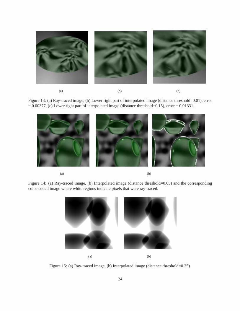
Figure 13: (a) Ray-traced image, (b) Lower right part of interpolated image (distance threshold=0.01), error= 0.00377, (c) Lower right part of interpolated image (distance threshold=0.15), error = 0.01331.

(a) (b)

Figure 14: (a) Ray-traced image, (b) Interpolated image (distance threshold=0.05) and the correspondingcolor-coded image where white regions indicate pixels that were ray-traced.

(a) (b)

Figure 15: (a) Ray-traced image, (b) Interpolated image (distance threshold=0.25).

24