international journal of engineering science address: [email protected] (j.b.r. loureiro)....

International Journal of Engineering Science 49 (2011) 397–410

Contents lists available at ScienceDirect

International Journal of Engineering Science

journal homepage: www.elsevier .com/locate / i jengsci

Scaling of turbulent separating flows

J.B.R. Loureiro a,⇑, A.P. Silva Freire b

a Scientific Division, Brazilian National Institute of Standards (INMETRO), Rio de Janeiro, Brazilb Mechanical Engineering Program (PEM/COPPE/UFRJ), C.P. 68503, 21945-970 Rio de Janeiro, Brazil

a r t i c l e i n f o a b s t r a c t

Article history:Received 21 May 2010Accepted 13 December 2010

Keywords:Law of the wallAdverse pressure gradientSeparationTurbulent boundary layerAsymptotic theory

0020-7225/$ - see front matter � 2010 Elsevier Ltddoi:10.1016/j.ijengsci.2010.12.001

⇑ Corresponding author.E-mail address: [email protected] (J.B.R. Lo

The present work investigates the scaling of the turbulent boundary layer in regions ofadverse pressure gradient flow. For the first time, direct numerical simulation and exper-imental data are applied to the theory presented in Cruz and Silva Freire [Cruz, D. O. A., &Silva Freire, A. P. (1998). On single limits and the asymptotic behaviour of separating tur-bulent boundary layers. International Journal of Heat and Mass Transfer, 41, 2097–2111] toexplain how the classical two-layered asymptotic structure reduces to a new structure con-sistent with the local solutions of Goldstein and of Stratford at a point of zero wall shearstress. The work discusses in detail the behaviour of an adaptable characteristic velocity(uR) that can be used in regions of attached as well as separated flows. In particular, uR

is compared to velocity scales based on the local wall shear stress and on the pressure gra-dient at the wall. This is also made here for the first time. A generalized law of the wall iscompared with the numerical and experimental data, showing good agreement. This law isshown to reduce to the classical logarithmic solution and to the solution of Stratford underthe relevant limiting conditions.

� 2010 Elsevier Ltd. All rights reserved.

1. Introduction

The early attempts at constructing theories for attached turbulent boundary layer flows in the asymptotic limit of largeReynolds number take as a central postulate the notion that the flow structure can be subdivided into two layers: (i) a wallviscous layer, in which the turbulent and laminar stresses are of comparable magnitude and (ii) a defect layer, in which thevelocity profile may be expressed in terms of a small perturbation to the external flow solution. Both original notions wereadvanced by Prandtl (1925) and von Kármán (1930) through dimensional analysis. They naturally lead to a universal solu-tion that has been shown by Millikan (1939) to have a logarithmic character and be dependent on velocity and length scalesbased on the friction velocity.

However, the action of a large adverse pressure gradient (APG) completely changes this picture, setting in a square-rootvelocity profile across the fully turbulent region that makes the previous scaling and asymptotic structures not suitable any-more (Stratford, 1959). In particular, at a point of flow separation the wall shear stress is zero so that none of the canonicaltheories (Bush & Fendell, 1972; Mellor, 1972; Yajnik, 1970) is valid.

Extensions of the Yajnik–Mellor (Mellor, 1972; Yajnik, 1970) theory to turbulent separation have been presented in lit-erature, notably by Melnik (1989), who proposes a formulation based on a two parameter expansion. One parameter of fun-damental importance to his developments, however, depends on a particular type of turbulent closure. This parameter isfurther used to regulate the order of magnitude of the pressure gradient term. Sychev and Sychev (1987) use the same

. All rights reserved.

ureiro).

http://dx.doi.org/10.1016/j.ijengsci.2010.12.001

mailto:[email protected]

http://dx.doi.org/10.1016/j.ijengsci.2010.12.001

http://www.sciencedirect.com/science/journal/00207225

http://www.elsevier.com/locate/ijengsci

398 J.B.R. Loureiro, A.P. Silva Freire / International Journal of Engineering Science 49 (2011) 397–410

theoretical framework of Yajnik (1970), Mellor (1972) and Bush and Fendell (1972) but consider an extra layer where theinternal friction forces, the pressure gradient and inertia forces balance each other. In their approach, no turbulence closureis required.

Many other different theories have been proposed in literature to explain the flow behaviour near to a separation point.However, no study satisfactorily elucidates the question of the scaling of mean velocity profiles in the entire domain of APGflows. As mentioned above, the appropriate near wall velocity scales for both attached and separated flows have long beenproposed by Prandtl (1925) and von Kármán (1930), and Stratford (1959), respectively. Regrettably, the conditions underwhich one must switch to the other and their impact on the local flow solution and asymptotic structure have not been ade-quately discussed in literature.

The present work uses a Kaplun-limit analysis (Cruz & Silva Freire, 1998) to correlate directly the asymptotic struc-ture of a separating flow with velocity and length scales (� = uR/ue,uR = reference velocity, ue = external flow velocity)based on a cubic algebraic equation that expresses the balance between pressure and internal friction forces in the innerregions of the flow and explains in physical terms the correct limiting behaviour of the local scales. For the first time,velocity and length scales based on the local wall shear stress, the local wall pressure gradient and on a combination ofboth are comprehensively compared with numerical and experimental data in regions of attached, separated and re-versed flow.

The work explains in a systematic way how the characteristic lengths of the wall viscous region �ðordð�Þ ¼ ordð1=�RÞ,R = Reynolds number = uel/m, l ¼ ðqu2

e=ðoxpÞwÞ;w ¼ wall conditionsÞ and of the fully turbulent region ~�ðordð~�Þ ¼ ordð�2ÞÞ de-fine an asymptotic structure that is valid throughout the flow region. Of special interest is an explanation about the relativechange in order of magnitude of the characteristic lengths at a separation point. The work also shows that in the reverse flowregion a y2-solution prevails over most of the near wall region. This finding is opposed to the results reported in Simpson(1983), who proposes a log-solution.

The validity domain of a local solution previously developed to describe the velocity profile in the fully turbulent region ofthe flow (Loureiro, Soares, Fontoura Rodrigues, Pinho, & Silva Freire, 2007; Loureiro, Pinho, & Silva Freire, 2007; Loureiro,Monteiro, Pinho, & Silva Freire, 2008) is compared with the characteristic flow regions defined by the presently identifiedasymptotic structure. This is also made here for the first time. The local solution satisfies the limiting behaviour for attached(log-solution) as well as separated (y1/2-solution) flows.

The current results are validated against three data sets: the flat-plate flows of Na and Moin (1998) and of Skote and Hen-nigson (2002) and the flow over a steep hill of Loureiro et al. (2007). These data were chosen for the very distinct geometry offlows they cover in addition to the possibility of analyzing the separation point region. The data of Na and Moin (1998) and ofSkote and Hennigson (2002) were obtained through a direct numerical simulation of the Navier–Stokes equations. Therefore,they are very detailed but for a low Reynolds number range. The data of Loureiro et al. (2007) were obtained through LDAmeasurements; they cover a higher Reynolds number range and furnish wall shear stress, mean velocity and turbulenceprofiles.

2. Relevant scales for separating flows

The above remarks concerning the changes in scaling laws will now be given a brief analytical explanation.

2.1. Characteristic scales for attached flows

The two-layered model established by Prandtl (1925), von Kármán (1930, 1939) for attached flows considers that acrossthe wall layer the total shear stress deviates just slightly from the wall shear stress. Hence, in the viscous layer a linear solu-tion u+ = y+ follows immediately with u+ = u/u⁄, y+ = y/(m/u⁄) and u� ¼

ffiffiffiffiffiffiffiffiffiffiffisw=q

p.

For the turbulence dominated flow region we may write:

oyst ¼ oyð�qu0v 0Þ ¼ 0: ð1Þ

A simple integration of the above equation implies that ord(u0) = ord(v0) = ord(u⁄), where we have clearly considered thevelocity fluctuations to be of the same order.

The analysis may proceed by taking as a closure assumption the mixing-length theory. A further equation integrationyields the classical law of the wall for a smooth surface:

uþ ¼ ,�1 ln yþ þ A; ð2Þ

where u+ = u/u⁄, y+ = y/(m/u⁄), , = 0.4, A = 5.0.

2.2. Characteristic scales for separated flows

The essential description of the physics of flow at a separation point has been given by Goldstein (1930, 1948) and byStratford (1959). The action of an arbitrary pressure rise in the inner layer distorts the velocity profile implying that the gra-dient of shear stress must now be balanced by the pressure gradient.

J.B.R. Loureiro, A.P. Silva Freire / International Journal of Engineering Science 49 (2011) 397–410 399

2.2.1. Viscous sublayerIn an attempt to elucidate the mathematical nature of some previously unknown laminar boundary layer solutions, Gold-

stein (1930, 1948) showed that if the fluid velocity at a separation point is approximated by a power-series in x and y, thenwhen some conditions are broken, the solution has an algebraic singularity. According to Goldstein’s analysis, the similaritycoordinate varies with x�1/4 and the solution expansion proceeds in powers of x1/4.

The papers of Goldstein consider p and oxp independent of y so that the canonical boundary layer equations can be usedand the external pressure gradient can be taken as a representative parameter. This is, of course, a false assumption, whichhas been rectified with the introduction of the triple-deck theory (see, e.g., Stewartson, 1974).

Goldstein, however, showed that at a point of zero skin-friction the velocity profile must follow a y2-profile at the wall.For turbulent flow, the fact that the local leading order equations must be dominated by viscous and pressure gradient ef-fects implies immediately that this result remains valid.

In fact, in the viscous region the local governing equation can be written as:

moyyu ¼ q�1oxp: ð3Þ

Two successive integrations of Eq. (3) and the fact that sw = 0, give:

uþ ¼ ð1=2Þyþ2; ð4Þ

with u+ = u/upm, y+ = y/(m/upm), upm = ((m/q)oxp)1/3.Note that in Eq. (4) the term oxp must be evaluated at y = 0. Hence, wall similarity solutions cannot be expressed in terms

of the external pressure gradient. In the following we refer to Eq. (4) as Goldstein’s solution.

2.2.2. Turbulent sublayerFor the turbulence dominated region, Stratford (1959) wrote:

oyst ¼ oxp: ð5Þ

Two successive integrations of Eq. (5) together with the mixing length hypothesis and, again, the fact that at a separationpoint sw = 0, give:

uþ ¼ ð2,�1Þyþ1=2; ð6Þ

with u+ and y+ defined as in Eq. (4).To find his solution Stratford used the condition y = 0, u = 0. Strictly speaking, this condition should not have been used

since Goldstein’s y2-expression is the solution that is valid at the wall. Stratford also incorporated an empirical factor – b(= 0.66) – to Eq. (6) to correct pressure rise effects on ,.

Thus, we may conclude that, at a separation point, ord(u0) = ord(v0) = ord(upm).

2.3. Characteristic scales for attached and separated flows

The relevant velocities and length scales in the wall region for flows away and close to a separation point are then (u⁄,m/u⁄) and (upm,m/upm), respectively.

The noticeable result is that both relevant velocity scales – u⁄ and upm – are contained in

�u0v 0 � q�1sw� �

� q�1oxp� �

y ¼ 0: ð7Þ

This equation is obtained through a first integration of the x-momentum equation. It represents the momentum balancein the near the wall region where the viscous and turbulent stresses are balanced by the local pressure gradient.

In the limiting cases sw� (y/q)(oxp) and sw� (y/q)(oxp), the scaling velocity tends to u⁄ and ((m/q)oxp)1/3, respectively,where oxp is to be considered at the wall.

To propose a characteristic velocity that is valid for the whole domain, Cruz and Silva Freire (1998, 2002) suggested toreduce Eq. (7) to an algebraic equation by considering ord(u0) = ord(v0) = ord(uR) and ord(y) = ord(m/uR). Thus, the referencevelocity, uR, is to be determined from:

u3R � q�1sw

� �uR � q�1m

� �oxp ¼ 0: ð8Þ

Eq. (8) always presents, at least, one real root. When three real roots are obtained, the highest root must be considered.

3. The method of kaplun, limits of equations, principal limits

In this section, part of the analysis of Cruz and Silva Freire (1998) is briefly repeated to establish a minimum condition fordiscussion. The following developments also introduce the correct flow scalings – ambiguously defined in Cruz and Silva Fre-ire (1998, 2002) – and a discussion on the flow asymptotic structure.


3.1. Asymptotic structure of an equilibrium turbulent boundary layer

Let us consider the problem of an incompressible turbulent flow over a smooth surface in a prescribed pressure distribu-tion. The time-averaged equations of motion – the continuity equation and the Reynolds equation – can be cast as:

oiui ¼ 0; ð9Þ

ujojui ¼ �q�1oip� �2oj u0ju0i

� �þ R�1

o2ui; ð10Þ

where the notation is classical. Thus, in a two-dimensional flow, (x1,x2) = (x,y) stands for a Cartesian coordinate system,(u1,u2) = (u,v) for the velocities, p for pressure and R (= uel/m) for the Reynolds number. The dashes are used to indicate a fluc-tuating quantity. In the fluctuation term, an overbar is used to indicate a time-average.

All mean variables are referred to the free-stream mean velocity, ue, and to the characteristic lengthl ¼ ðqu2

e=ðoxpÞwÞ; ðw ¼ wall conditionsÞ. The velocity fluctuations, on the other hand, are referred to the characteristic veloc-ity uR defined by Eq. (8) so that � = uR/ue.

The purpose of perturbation methods is to find approximate solutions to Eqs. (9) and (10) that are valid when one ormore of the variables or parameters in the problem are small or large. Provided the small parameters are taken to be � andR�1, one can clearly see that in the limits �? 0 or R ?1 terms containing high derivatives in the equation are lost. Thereduction in the order of the equation means that some of the boundary conditions will be lost as well, so that the approx-imations fail in places where they were to be imposed. One must then seek local approximations in terms of local scaledvariables that complement each other and can be matched in some common domain of validity. The essentials behind‘‘inner-outer’’ or ‘‘matched asymptotic’’ approximations involve the concepts of limit process, domain of validity, overlapand matching.

The present account on perturbation methods is based on the results of Kaplun (1967), Lagerstrom and Casten (1972) andLagerstrom (1988). For further details, the reader is referred to the original sources. In the following, we use the topology onthe collection of order classes as introduced by Meyer (1967). For positive, continuous functions of a single variable � definedon ð0; 1�, let ord g denote the class of equivalence introduced in Meyer.

Definition. (Lagerstrom, 1988). We say that f(x,�) is an approximation to g(x,�) uniformly valid to order d(�) in a convex setD(f is a d-approximation to g), if:

lim f ðx; yÞ � gðx; yÞð Þ=dð�Þ ¼ 0; �! 0; uniformly for x in D: ð11Þ

The function d(�) is sometimes called a gauge function.

The essential idea of the single limit process g-limit is to study the limit as �? 0 not for fixed x near a singularity point xd,but for x tending to xd in a definite relationship to � specified by a function g (�). Taking without any loss of generality xd = 0,we define:

xg ¼ x=gð�Þ; G xg; ��

¼ Fðx; �Þ; ð12Þ

with g(�) defined in N(= space of all positive continuous functions on ð0; 1�).

Definition of Kaplun limit. [Meyer, 1967] If the function G(xg;+0) = lim G(x g;�), �? 0, exists uniformly on {xg/jx gj > 0};then we define limg F(x;�) = G(xg;+0).

Thus, if g ? 0 as �? 0, then, in the limit process, x ? 0 also with the same rate of g, so that x/g tends to a non-zero limitvalue.

To investigate the asymptotic structure of the turbulent boundary layer we consider:

uðx; yÞ ¼ u1ðx; yÞ þ �u2ðx; yÞ;vðx; yÞ ¼ gv1ðx; yÞ;pðx; yÞ ¼ p1ðx; yÞ;

ð13Þ

and the following transformation:

y ¼ yg ¼ y=gð�Þ; uiðx; ygÞ ¼ uiðx; yÞ: ð14Þ

Upon substitution of Eqs. (13) and (14) into Eqs. (9) and (10) and depending on the order class of g we then find the fol-lowing formal limits:

continuity equation:

ord v i x; yg

� �� ¼ ord gui x; yg

� �� : ð15Þ


x-momentum equation:

ordg ¼ ord1 : u1oxu1 þ v1oyg u1 þ oxp1 ¼ 0; ð16Þord�2 < ordg < ord1 : u1oxu1 þ v1oyg u1 þ oxp1 ¼ 0; ð17Þord�2 ¼ ordg : u1oxu1 þ v1oyg u1 þ oxp1 ¼ �oyg u01v 01; ð18Þord 1=�2R

� �< ordg < ord�2 : oyg u01v 01 ¼ 0; ð19Þ

ord 1=�2R� �

¼ ordg : �oyg u01v 01 þ o2yg

u1 ¼ 0; ð20Þ

ordg < ord 1=�2R� �

: o2yg

u1 ¼ 0: ð21Þ

y-momentum equation:

ordg ¼ ord1 : u1oxv1 þ v1oyg v1 þ oyg p1 ¼ 0; ð22Þordg < ord1 : oyg p1 ¼ 0: ð23Þ

The set of Eqs. (15)–(23) is referred to by Kaplun as the ‘‘splitting’’ of the differential equations. The splitting is a formalproperty of the equations, obtained onto passage of the g-limit process. Thus, to every order of g a correspondence isinduced, limg? associated equation, on that subset of N for which the associated equation exists.

Definition. The formal local domain of an associated equation E is the set of orders g such that the g-limit process applied tothe original equation yields E.

One should note that passage of the g-limit establishes a hierarchy within the associate equations. Some equations aremore ‘‘complete’’ or ‘‘rich’’ than others in the sense that application of the g-limit process to them will result in otherassociated equations, but neither of them can be obtained from any of the other associated equations. Eqs. (18) and (20) aresuch ‘‘rich’’ equations. Limit-processes which yield ‘‘rich’’ equations were called by Kaplun principal limit-processes. Theseideas can be given a more strict interpretation by introducing Kaplun’s concept of equivalent in the limit for a given set ofequations for a given point (g,d) of the (N,N) product space.

Given any two associated equations E1 and E2, Kaplun defines:

R xg; ��

¼ E1 xg; ��

� E2 xg; ��

; ð24Þ

where � denotes a small parameter.According to Kaplun (1967), R should be interpreted as an operator giving the ‘‘apparent force’’ that must be added to E2

to yield E1.

Definition of equivalence in the limit. [Kaplun, 1967] Two equations E1 and E2 are said to be equivalent in the limit for agiven limit-process, limg, and to a given order, d (�), if:

R xg; ��

=dð�Þ ! 0; as �! 0; xg fixed: ð25Þ

The following definitions are now possible.

Definition of formal domain of validity. The formal domain of validity to order d of an equation E of formal local domain Dis the set De = D [ D0is, where D0is are the formal local domains of all equations E0i such that E and E0i are equivalent in D0i toorder d.

Definition of principal equation. An equation E of formal local domain D, is said to be principal to order d if:

(i) One can find another equation E0, of formal local domain D0, such that E and E0 are equivalent in D0 to order d.(ii) E is not equivalent to order d to any other equation in D.

An equation which is not principal is said to be intermediate.The intermediate equation, Eq. (21), together with the boundary condition u1ðx;0Þ ¼ 0, imply that the near wall solution

is u1ðx; ygÞ ¼ yg. This solution has to be contained by the principal solution furnished by Eq. (20). The outer flow equations, onthe other hand, imply that u1ðx; ygÞ ¼ ueðx; yÞ. Thus, we appear to be faced by a dilemma for the inner solution is unboundedin the limit yg !1 and hence no matching can be achieved with the bounded outer solution. In fact, the matching processthat involves the inner and outer solutions is to be performed in a region dominated by Eq. (19). As it turns out, Eq. (19)yields a solution with a limiting logarithmic behaviour that bridges a inner solution of order � to the outer solution of orderunity through the relationship � = ord(ln�1 R). This problem has been investigated by many authors (see, e.g., Afzal, 1976;


Izakson, 1937; Millikan, 1939; Tennekes, 1973; Yajnik, 1970) and is sometimes called a ‘generation gap’ (Mellor, 1972). Animportant additional implication is the deduction of an algebraic relationship that can be used for the prediction of the localskin-friction.

Nothing in the formal procedure that led to Eqs. (16)–(21) indicated that a inner solution with leading order � wasneeded. Only an inspection of the local solutions and of the matching conditions can reveal its existence. Terms that arefound from inspection of formally higher order terms are referred to in literature as switchback terms; they are quite com-mon in singular perturbation problems.

Since the leading order solution in the inner regions of the flow is ord (�), it follows that (1/�2 R) has to be replaced by (1/�R) in Eqs. (19)–(21) so that the inner region principal equation is given by

ord ð1=�RÞ ¼ ordg : �oyg u01v 01 þ o2yg

u1 ¼ 0: ð26Þ

Therefore, the principal equations to the turbulent boundary layer problem are Eqs. (18), (26) and (22). The relevantscales �2 and 1/� R coincide with the scales proposed by Sychev and Sychev (1987) for the description of their two internallayers. These authors also consider a third layer. However, in the interpretation of Kaplun limits, this is not necessary for onlyredundant information is conveyed. An important point to be raised here is the nature of the principal equation in y-direc-tion. To solve the boundary layer equations one needs to consider Eq. (22), instead of the Prandtl formulation oyp = 0. Bydoing this, the boundary layer approximation becomes a self-contained theory in the sense that any type of viscous-inviscidinteractive process becomes unnecessary.

To relate the formal properties of equations described above to the actual problem of determining the uniform domain ofvalidity of solutions, Kaplun (1967) advanced two assertions, the Axiom of Existence and the Ansatz about domains of valid-ity. These assertions constitute primitive and unverifiable assumptions of perturbation theory.

Axiom of existence. [Kaplun, 1967] If equations E and E0 are equivalent in the limit to the order d for a certain region, thengiven a solution S of E which lies in the region of equivalence of E and E0, there exists a solution S0 of E0 such that as �? 0,jS � S0j/d ? 0, in the region of equivalence of E and E0.

In simple terms, the axiom states that there exists a solution S0 of E0 such that the ‘‘distance’’ between S and S0 is of thesame order of magnitude of that between E and E0. In perturbation methods, a common approach is to consider the existenceof certain limits of the exact solution or expansions of a certain form. This is normally a sufficient condition to find the asso-ciated equations and to consider that the axiom is satisfied (Kaplun, 1967).

To the axiom of existence there corresponds an Ansatz; namely that there exists a solution S of E which lies in the regionof equivalence of E and E0. More explicitly, we write.

Ansatz about domains of validity. [Kaplun, 1967] An equation with a given formal domain of validity D has a solutionwhose actual domain of validity corresponds to D.

The word ‘‘corresponds to’’ in the Ansatz was assumed by Kaplun to actually mean ‘‘is equal to’’; this establishes the linkwe needed between the ‘‘formal’’ properties of the equation and the actual properties of the solution. According to Kaplun,the Ansatz can always be subjected to a canonical test which consists in exhibiting a solution S0 of E0 which lies in the region ofequivalence of E and E0 and is determined by the boundary conditions that correspond to S. Because the heuristic nature ofthe Axiom and of the Ansatz, comparison to experiments will always be important for validation purposes. The theory, how-ever, as implemented through the above procedure, is always helpful in understanding the matching process and in con-structing the appropriate asymptotic expansions.

The overlap domain of Eqs. (18) and (26) can now be determined through Rðxg; �Þ by taking d(�) = �a. Then upon substi-tuting E1 by Eq. (18), E2 by Eq. (26) and passing the limit as � tends to zero, one finds:

Doverlap ¼ g=ord ð�1þaRÞ�1< ordg < ord ð�2þaÞ

n o: ð27Þ

The two principal equations then provide approximate solutions that are accurate to order (�amax ) where:

amax ¼ �ð1=2Þ ðln R= ln �Þ þ 3ð Þ: ð28Þ

3.2. Asymptotic structure of a separating turbulent boundary layer

As the flow approaches a separation point, however, we have already seen that the structure depicted by Eqs. (15)–(26)breaks down. To account for the flow behaviour, we must consider Kaplun limits in x-direction.

Let us define:

x ¼ xD ¼ x=Dð�Þ;y ¼ yg ¼ y=gð�Þ;uiðxD; ygÞ ¼ uiðx; yÞ:

ð29Þ

with D(�) and g(�) defined on N.


The idea is to approach the separation point by taking simultaneously the g- and D-limits at a fixed rate f = D/g = ord(1).Note that in regions where ord(D) = ord(�), ord(u⁄) = ord(upm); under this condition, ord(�2) = ord(1/�R).

The resulting flow structure is given by

continuity equation:

ord v i x; yg

� �� ¼ ord ui x; yg

� �� : ð30Þ

x-momentum equation:

ordD ¼ ord1 : u1oxD u1 þ v1oyg u1 þ oxD p1 ¼ 0; ð31Þord�2 < ordD < ord1 : u1oxD u1 þ v1oyg u1 þ oxD p1 ¼ 0; ð32Þ

ord�2 ¼ ordD : u1oxD u1 þ v1oyg u1 þ oxD p1 ¼ �oxD u012 � oyg u01v 01 þ o2

xDu1 þ o2

ygu1; ð33Þ

ordD < ord�2 : o2xD

u1 þ o2yg

u1 ¼ 0: ð34Þ

y-momentum equation:

ordD ¼ ord1 : u1oxD v1 þ v1oyg v1 þ oyg p1 ¼ 0; ð35Þord�2 < ordD < ord1 : u1oxD v1 þ v1oyg v1 þ oyg p1 ¼ 0; ð36Þ

ord�2 ¼ ordD : u1oxD v1 þ v1oyg v1 þ oyg p1 ¼ �oxD u01v 01 � oygm012 þ o2

xDv1 þ o2

ygv1; ð37Þ

ordD < ord�2 : o2xD

v1 þ o2yg

v1 ¼ 0: ð38Þ

The principal equations are Eqs. (33) and (37). They show that near to a separation point the two principal equations, Eqs.(18) and (26), merge giving rise to a new structure dominated basically by two regions: a wake region (ord(g),ord(D) > �2)and a viscous region (ord(g),ord(D) < �2). These are regions governed, of course, by intermediate equations. Thus, matchingbetween them cannot be achieved directly. The disappearance of the region dominated solely by the turbulence effects isnoted. The principal equations recover the full Reynolds averaged Navier–Stokes equations.

The system of Eqs. (31)–(38), indicates that the pressure gradient effects become leading order effects for orders higherthan ord(�2) = ord(D). Thus, at about ord(x/l) = ord(D) = ord(�) we should have ord(u⁄) = ord(upm), so that these terms fur-nish first order corrections to the mean velocity profile.

4. Near wall solution

To find the relevant near wall solution of the flow, we consider the approximate equation in the domain bounded byord(�2) and ord (1/�R), the fully turbulent region. This equation is given by

ð,yÞoyu ¼ffiffiffiffiffiffiffiffiffiffiffiffiffiffiffiffiffiffiffiffiffiffiffiffiffiffiffiffiffiffiffiffiffiffiffiffiffiffiffiffiffiffiffiffiq�1swð Þ þ ðq�1oxpÞy

q; ð39Þ

where the mixing length hypothesis has been considered.A double integration of Eq. (39) furnishes:

u ¼ 2,�1D1=2w þ ,�1u� ln D1=2

w � u��

D1=2w þ u�

� �� þ C; ð40Þ

with Dw = q�1sw + (q�1oxp)y.Eq. (40) can be seen as a generalization of the classical law of the wall for separating flows. In the limiting case

(oxp)y� sw, Eq. (39) reduces to the logarithmic law. Near a point of separation Stratford’s solution is recovered.Eq. (40) can be used indistinctly in all flow regions – including regions of reversed flow – provided its domain of validity is

respected and appropriate integration constants are determined. Many other different treatments of the lower boundarycondition can be appreciated in literature. Loureiro et al. (2007), for example, have investigated the numerical predictionof flows over two-dimensional, smooth, steep hills according to the above formulation and the formulations of Mellor(1966) and of Nakayama and Koyama (1984). The standard j–� model was then used to close the averaged Navier–Stokesequations. The results are shown to vary greatly.

An extension of Eq. (40) to flows over rough walls has been introduced by Loureiro et al. (2008), Loureiro, Monteiro, Pinho,and Silva Freire (2009) and Loureiro and Silva Freire (2009).

5. Results: experimental and numerical validation

The structure of a separating turbulent boundary layer, as described above, will be tested against the DNS data of Na andMoin (1998) and Skote and Hennigson (2002) and the experimental data of Loureiro et al. (2007). These are accounts of the

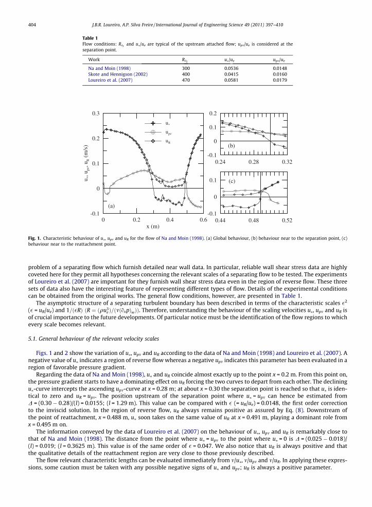
Table 1Flow conditions: Rd2 and u⁄/ue are typical of the upstream attached flow; upm/ue is considered at theseparation point.

Work Rd2 u⁄/ue upm/ue

Na and Moin (1998) 300 0.0536 0.0148Skote and Hennigson (2002) 400 0.0415 0.0160Loureiro et al. (2007) 470 0.0581 0.0179

0 0.2 0.4 0.6x (m)

-0.1

0

0.1

0.2

0.3

u *, u pν

, uR (

m/s

)

u*

upν

uR

0.44 0.48 0.52-0.1

0

0.1

0.24 0.28 0.32-0.1

0

0.1

0.2

(a)

(b)

(c)

Fig. 1. Characteristic behaviour of u⁄, upm and uR for the flow of Na and Moin (1998). (a) Global behaviour, (b) behaviour near to the separation point, (c)behaviour near to the reattachment point.


problem of a separating flow which furnish detailed near wall data. In particular, reliable wall shear stress data are highlycoveted here for they permit all hypotheses concerning the relevant scales of a separating flow to be tested. The experimentsof Loureiro et al. (2007) are important for they furnish wall shear stress data even in the region of reverse flow. These threesets of data also have the interesting feature of representing different types of flow. Details of the experimental conditionscan be obtained from the original works. The general flow conditions, however, are presented in Table 1.

The asymptotic structure of a separating turbulent boundary has been described in terms of the characteristic scales �2

(� = uR/ue) and 1=ð�RÞ ðR ¼ ðqu3e Þ=ðmðoxpÞwÞÞ. Therefore, understanding the behaviour of the scaling velocities u⁄, upm and uR is

of crucial importance to the future developments. Of particular notice must be the identification of the flow regions to whichevery scale becomes relevant.

5.1. General behaviour of the relevant velocity scales

Figs. 1 and 2 show the variation of u⁄, upm and uR according to the data of Na and Moin (1998) and Loureiro et al. (2007). Anegative value of u⁄ indicates a region of reverse flow whereas a negative upm indicates this parameter has been evaluated in aregion of favorable pressure gradient.

Regarding the data of Na and Moin (1998), u⁄ and uR coincide almost exactly up to the point x = 0.2 m. From this point on,the pressure gradient starts to have a dominating effect on uR forcing the two curves to depart from each other. The decliningu⁄-curve intercepts the ascending upm-curve at x = 0.28 m; at about x = 0.30 the separation point is reached so that u⁄ is iden-tical to zero and uR = upm. The position upstream of the separation point where u⁄ = upm can hence be estimated fromD = (0.30 � 0.28)/(l) = 0.0155; (l = 1.29 m). This value can be compared with � (= uR/ue) = 0.0148, the first order correctionto the inviscid solution. In the region of reverse flow, uR always remains positive as assured by Eq. (8). Downstream ofthe point of reattachment, x = 0.488 m, u⁄ soon takes on the same value of uR at x = 0.491 m, playing a dominant role fromx = 0.495 m on.

The information conveyed by the data of Loureiro et al. (2007) on the behaviour of u⁄, upm and uR is remarkably close tothat of Na and Moin (1998). The distance from the point where u⁄ = upm to the point where u⁄ = 0 is D = (0.025 � 0.018)/(l) = 0.019; (l = 0.3625 m). This value is of the same order of � = 0.047. We also notice that uR is always positive and thatthe qualitative details of the reattachment region are very close to those previously described.

The flow relevant characteristic lengths can be evaluated immediately from m/u⁄, m/upm and m/uR. In applying these expres-sions, some caution must be taken with any possible negative signs of u⁄ and upm; uR is always a positive parameter.

-0.8 -0.4 0 0.4 0.8x (m)

-0.004

-0.002

0

0.002

0.004

0.006

0.008

u *, u pν

, uR (

m/s

)

u*

upν

uR

(a)

0 0.02 0.04 0.06-0.002

0

0.002

0.004

0.006(b)

0.32 0.36 0.4 0.44-0.002

-0.001

0

0.001

0.002

0.003

(c)

Fig. 2. Characteristic behaviour of u⁄, upm and uR for the flow of Loureiro et al. (2007). (a) Global behaviour, (b) behaviour near to the separation point, (c)behaviour near to the reattachment point.

0 0.1 0.2 0.3 0.4 0.5 0.6x (m)

0.00001

0.00010

0.00100

0.01000

Fig. 3. Diagram of the asymptotic structure of the turbulent boundary layer for separating and reattaching flows; data of Na and Moin (1998).

-0.4 -0.2 0 0.2 0.4 0.6 0.8x (m)

0.00001

0.00010

0.00100

0.01000

0.10000

Fig. 4. Diagram of the asymptotic structure of the turbulent boundary layer for separating and reattaching flows; data of Loureiro et al. (2007), Loureiroet al. (2007).


5.2. General behaviour of the relevant length scales

The asymptotic structure of the flow is illustrated through Figs. 3 and 4, where the thickness scalings (�R)�1 and �2 areshown in semi-log form for the data of Na and Moin (1998) and Loureiro et al. (2007), respectively. Far upstream of the sep-aration point a classical two layered structure is found with thickness � (= (�R)�1) representing a leading order balance


between the laminar and turbulent stresses (Eq. (26)). Thickness ~� (= �2) represents the balance between the turbulent stressand inertial effects (Eq. (18)). As the separation point is approached, � and ~� exhibit opposed variations. The steady increaseof � together with the steady decrease of ~� provoke a continuous narrowing of the turbulence dominated region up to thepoint where it becomes completely extinguished. This happens exactly at the position of flow separation. The implicationis that at this position the near wall flow solution is viscous dominated so that a Goldstein solution prevails up to y � �.On the other hand, the region ord(g) = ord(y/l) = ord(�2), defines the flow position where Stratford’s solution is supposedto hold. Above this point, an inertia dominated solution is to be found.

In the region of reverse flow, the dominant roles of � and ~� are inverted. The negative wall shear stress combined with thelow pressure gradient at the wall make �� ~�. The asymptotic implication is that in the region of reverse flow, sometimesreferred to in literature as a ‘‘dead-air’’ area, the solution is largely viscous dominated. Thus, a Goldstein velocity profileis expected to be a good approximation up to large distances from the wall. A discussion on the ability of Goldstein’s solutionto represent the motion in regions of reverse flow is made next (see, for example, Fig. 7).

The roles of � and ~� is again inverted downstream of the point of flow reattachment, when the order ~�� is restored. Theflow then settles back to the canonical asymptotic structure of the turbulent boundary layer with a reestablishment of thelogarithmic region.

5.3. Evaluation of the solutions of Goldstein and of Stratford

An inspection of the flow behaviour near to a point of separation is of particular interest. The data of Na and Moin (1998)are shown in Fig. 5(a) and (b) in wall coordinates u+ and y+(= u/uR and y uR/m). The solutions of Goldstein and of Stratford aregiven respectively by u+ = 0.484 (y+)2 and u+ = 4.125 (y+)1/2 � 4.332 in the ranges 0.028 � y+� 1.33 and 1.54�y+� 14.82.This is consistent with the present asymptotic modeling of the problem whereby the two solutions are to be matched in aflow region of ord(1/�R) = ord(�2), that is ord(y+) = 1.

5.4. Local mean velocity distributions

The near wall solution furnished by Eq. (40) will now be tested against the data of Na and Moin (1998), Loureiro et al.(2007) and Skote and Hennigson (2002). For later reference we notice that Eq. (4) at a point where sw – 0 is given by

Fig. 5.Stratfor

uþ ¼ ð1=2Þuþpm3yþ2 þ uþ�

2yþ; ð41Þ

with uþ ¼ u=uR;uþpm ¼ upm=uR;uþ� ¼ u�=uR and y+ = yuR/m.The streamwise development of the Na and Moin mean velocity profiles is shown in Fig. 6 in wall coordinates. Six stations

have been considered, at positions x=d�i ¼ 50;100;158 (position of flow separation), 200, 250 and 257 (position of flow reat-tachment); d�i = inlet displacement thickness. The results at the exact positions of flow separation and reattachment wereinterpolated directly from the original data source.

Fig. 6(a) and (b) show the profiles upstream of the flow separation. The local solutions given by Eqs. (40) and (41) are alsoshown. Because the data of Na and Moin are obtained for a very low Reynolds number and under a non-zero pressure gra-dient condition, the profiles in the logarithmic regions of the flow never really approach the standard law of the wall profilewith A = 5 (Eq. (2)). The solution of Goldstein (Eq. (41)) exhibits a very good agreement to the DNS solution up to y+ = 4.5. Thelog solution is also a very good match to the DNS data provided C is taken as 16.4 ðx=d�i ¼ 50Þ and 9:7ðx=d�i ¼ 100Þ. This con-stant corresponds to the patching point y+ � 8. The asymptotic limits 1/�R and �2 are noted to define an overlap region thatcontinuously shrinks as the separation point is approached.

At the separation point (Fig. 6(c)), Goldstein’s solution is a good approximation up to about y+ = 1.5 (see also Fig. 5(a)); thelog solution appears to be a reasonable approximation up to y+ = 45. This value should be compared with the upper bound fora Stratford approximation, y+ � 15 (Fig. 5(b)). The overlap domain is reduced to ord(1/�R) = ord(�2).

1 2 3 40

4

8

12

0 0.4 0.8 1.2 1.6 20

0.2

0.4

0.6

0.8

1

u+

(a) (b)

Velocity profiles at the point of zero wall shear stress for the flow of Na and Moin (1998). (a) Solution of Goldstein (u+ = 0.484 (y+)2), (b) solution ofd (u+ = 4.125 (y+)1/2 � 4.332).

Fig. 7. Detail of mean velocity profiles in the region of reverse flow (Na & Moin, 1998). (a) x=d�i ¼ 200, (b) 250, d�i = inlet displacement thickness.

Fig. 6. Mean velocity profiles in wall coordinates according to the data of Na and Moin (1998). (a) x=d�i ¼ 50, (b) 100, (c) 158 (position of flow separation),(d) 200, (e) 250, (f) 257 (position of flow reattachment), d�i = inlet displacement thickness.



The velocity profiles in the reverse flow region are shown in Fig. 6(d) and (e). The dominant role of the viscous effects hadalready been illustrated in Figs. 3 and 4. Here, we see that Eq. (41) is a very good solution approximation up to about y+ = 1.4(for flow details see Fig. 7(a) and (b)). As a first approximation, the point y+ = 1 can actually be used in Fig. 6(d) and Fig. 6(e)to patch Eqs. (41) and (40). Eq. (40) is not a good solution in the interval 0.22 < y+ < 1, so that patching Eq. (41) directly to Eq.(40) offers a good simplifying procedure. In fact, Simpson (1983) remarked that for y/N < 0.02 (N = distance from the wall tothe maximum backflow velocity) a Goldstein solution should be appropriate. Farther from the wall, he argued turbulent ef-fects are supposed to play a role so that a log profile would be in order. He then suggests a solution of the form:

U= UNj j ¼ A y=N � lnðjy=NjÞ � 1ð Þ � 1; A ¼ 0:3: ð42Þ

Unfortunately, constant A in this expression has been assigned many values according to different authors. Skote andHennigson (2002) show that Eq. (42) furnishes a very poor agreement with their data. The same trend can be observed inFig. 7(b). The conclusion is that a Goldstein solution gives the best reverse flow representation in the interval y+ < 0.37.

Just downstream of the reattachment point (Fig. 6(f)), the velocity profile behaves much in the same way as near or at theseparation point. Goldstein and Stratford solutions apply and the log region starts to become dominant again.

The data of Loureiro et al. (2007) are shown in Fig. 8(a) and (b) where both measuring stations have been considered inregions of reverse flow. Station x/H = 0.5(H = hill height) is located just past the point of separation; in fact, up to y+ = 1.65,the flow is reverse. Eq. (41) is noted to be a good representation of the flow up to y+ = 2. Eq. (40) also gives a good represen-tation of the flow in this region provided C = �0.76. At station x/H = 3.75, the solution of Goldstein yields values slightly high-er than the measured profile. For the outer flow region, Eq. (40) gives good predictions on the condition that C = �27.

A further characterization of reverse and attached flows in given in Fig. 9(a) and (b) according to the DNS data of Skoteand Hennigson (2002). Again, in reverse flow (Fig. 9(a)), Eq. (41) is observed to furnish very good results for y+ < 1. On theother hand, the agreement of Eq. (40) with the outer region DNS data is very poor. Fig. 9(b) shows the mean velocity profiledownstream of the separation bubble; one can easily note that the flow has recovered a log region, which can be well de-scribed by Eq. (40) in 1.7 < y+ < 55 (C = �29).

The values of the integration constant in Eq. (40) are shown in Table 2 for the flow conditions considered in this work.

Fig. 8. Mean velocity profiles in wall coordinates according to the data of Loureiro et al. (2007). (a) x/H = 0.5, (b) 3.75, H = hill height.

Fig. 9. Mean velocity profiles in wall coordinates according to the data of Skote and Hennigson (2002). (a) x/d⁄ = 300, (b) 500.

Table 2Parameter C for the various flow conditions.

Work Station C

Na and Moin (1998) 50 16.4100 9.7158 �5.4200 �16250 �6.6257 �4

Loureiro et al. (2007) 0.5 �0.763.75 �27

Skote and Hennigson (2002) 300 �29500 5.9


6. Final remarks

In the first part of the work, a direct application of Kaplun limits to the equations of motion has shown how the canonicaltwo-layered asymptotic structure of the turbulent boundary layer reduces to a one-layered structure at a point of zero wallshear stress. This change in structure is provoked by a change in the scaling parameters that must account for the shearstress and pressure gradient effects at the wall. In fact, the procedure of Kaplun has been supplemented by a scaling algebraicequation that has been derived from the first principles. This is an important feature of the present analysis: the equationthat is used to furnish the local velocity and length scales has been derived directly from the equations of motions.

Some authors have suggested in the past that the external pressure gradient should be used to define the reference veloc-ity and length scales of a separating flow, in which case one should have upm = ((m/q)(oxp)e)1/3, l ¼ ðqu2

e=ðoxpÞeÞ, (e = externalconditions). For the wall region, the present results have proved otherwise. The solutions of Goldstein and Stratford shown inFig. 5 imply that in the definition of the wall layer scaling the wall pressure gradient must be used. Here, a correct scalingprocedure based on the inner wall conditions has been exhaustedly demonstrated by the global asymptotic structure of theflow as well as by the local mean velocity solutions.

The numerical computation of turbulent flows always requires the specification of very fine meshes in the near wall re-gion. To overcome this problem, procedures that resort to local approximate analytical solutions have commonly been devel-oped in literature. These procedures can be applied to numerical simulations based on Reynolds Averaged Navier–Stokesequations (RANS) or Large Eddy simulation (LES) methods and use expressions with the form of Eq. (40) to bridge a less re-fined outer solution directly to the wall.

The great problem with these procedures is the appearance of numerical instabilities, resulting from the explicit methodsthat are used to evaluate the wall functions. In algorithms that adopt temporal integration to minimize the uncertainties inthe specification of the initial conditions, the instabilities associated with the use wall-functions are amplified, demandingthe use of special methods to achieve numerical stabilization. The present results identify the correct scales to be used insuch methods, showing that near to a separation point u⁄ must be switched to upm. In addition, the present results show thatuR can be used throughout the flow domain.

Acknowledgments

APSF is grateful to the Brazilian National Research Council (CNPq) for the award of a Research Fellowship (Grant No303982/2009-8). The work was financially supported by CNPq through Grants No 473588/2009-9 and by the Rio de JaneiroResearch Foundation (FAPERJ) through Grant E-26/170.005/2008. JBRL is thankful to the Brazilian National Research Council(CNPq) for the financial support to this research through Grant 475759/2009-5.

References

Afzal, N. (1976). Millikan’s arguments at moderately large Reynolds number. Physics of Fluids, 19, 600–602.Bush, W. B., & Fendell, F. E. (1972). Asymptotic analysis of turbulent channel flow and boundary-layer flow. Journal of Fluid Mechanics, 56, 657.Cruz, D. O. A., & Silva Freire, A. P. (1998). On single limits and the asymptotic behaviour of separating turbulent boundary layers. International Journal of Heat

and Mass Transfer, 41, 2097–2111.Cruz, D. O. A., & Silva Freire, A. P. (2002). Note on a thermal law of the wall for separating and recirculating flows. International Journal of Heat and Mass

Transfer, 45, 1459–1465.Goldstein, S. (1930). Concerning some solutions of the boundary layer equations in hydrodynamics. Proceedings of the Cambridge Philosophical Society, 26,

1–18.Goldstein, S. (1948). On laminar boundary-layer flow near a position of separation. Quarterly Journal of Mechanics and Applied Mathematics, 1, 43–69.Izakson, A. (1937). On the formula for the velocity distribution near walls. Technical Physics USSR IV, 155–162.Kaplun, S. (1967). Fluid mechanics and singular perturbations. Academic Press.Lagerstrom, P. A. (1988). Matched asymptotic expansions. Heidelberg: Springer-Verlag.Lagerstrom, P. A., & Casten, R. G. (1972). Basic concepts underlying singular perturbation techniques. SIAM Review, 14, 63–120.


Loureiro, J. B. R., Monteiro, A. S., Pinho, F. T., & Silva Freire, A. P. (2008). Water tank studies of separating flow over rough hills. Boundary-Layer Meteorology,129, 289–308.

Loureiro, J. B. R., Monteiro, A. S., Pinho, F. T., & Silva Freire, A. P. (2009). The effect of roughness on separating flow over two-dimensional hills. Experiments inFluids, 46, 577–596.

Loureiro, J. B. R., Pinho, F. T., & Silva Freire, A. P. (2007). Near wall characterization of the flow over a two-dimensional steep smooth hill. Experiments inFluids, 42, 441–457.

Loureiro, J. B. R., & Silva Freire, A. P. (2009). Note on a parametric relation for separating flow over a rough hill. Boundary-Layer Meteorology, 131, 309–318.Loureiro, J. B. R., Soares, D. V., Fontoura Rodrigues, J. L. A., Pinho, F. T., & Silva Freire, A. P. (2007). Water tank and numerical model studies of flow over steep

smooth two-dimensional hills. Boundary-Layer Meteorology, 122, 343–365.Mellor, G. L. (1966). The effects of pressure gradients on turbulent flow near a smooth wall. Journal of Fluid Mechanics, 24, 255–274.Mellor, G. L. (1972). The large Reynolds number, asymptotic theory of turbulent boundary layers. International Journal of Engineering Science, 10, 851–873.Melnik, R. E. (1989). An asymptotic theory of turbulent separation. Computers and Fluids, 15, 165–184.Meyer, R. E. (1967). On the approximation of double limits by single limits and the Kaplun extension theorem. Journal of the Institute of Mathematics and its

Applications, 3, 245–249.Millikan, C. B. (1939). A critical discussion of turbulent flow in channels and tubes. In Proceedings of the 5th international congress on applied mechanics. NY:

John Wiley.Nakayama, A., & Koyama, H. (1984). A wall law for turbulent boundary layers in adverse pressure gradients. AIAA Journal, 22, 1386–1389.Na, Y., & Moin, P. (1998). Direct numerical simulation of a separated turbulent boundary layer. Journal of Fluid Mechanics, 374, 379–405.Prandtl, L. (1925). Über die ausgebildete turbulenz. ZAMM, 5, 136–139.Simpson, R. L. (1983). A model for the backflow mean velocity profile. AIAA Journal, 21, 142–143.Skote, M., & Hennigson, D. S. (2002). Direct numerical simulation of a separated turbulent boundary layer. Journal of Fluid Mechanics, 471, 107–136.Stewartson, K. (1974). Multistructured boundary layers on flat plates and related bodies. Advances in Applied Mechanics, 14, 145–239.Stratford, B. S. (1959). The prediction of separation of the turbulent boundary layer. Journal of Fluid Mechanics, 5, 1–16.Sychev, V. V., & Sychev, V. V. (1987). On turbulent boundary layer structure. Prikladnaia Matematika i Mekhanika-USSR, 51, 462–467.Tennekes, H. (1973). The logarithmic wind profile. Journal of the Atmospheric Sciences, 30, 234–238.von Kármán, Th. (1930). Mechanische aehnlichkeit und turbulenz. In Proceedings of the 3rd international congress for applied mechanics, Stockholm.von Kármán, Th. (1939). Transactions of the American Society for Mechanical Engineering, 61, 705.Yajnik, K. S. (1970). Asymptotic theory of turbulent shear flow. Journal of Fluid Mechanics, 42, 411–427.

international journal of engineering science address: [email protected] (j.b.r. loureiro)....

Documents