n. f. loureiro - ompuserpages.irap.omp.eu/~frincon/houches/loureiro.pdf · an introduction to...

An Introduction to Magnetic Reconnection �

N. F. LOUREIRO Instituto de Plasmas e Fusão Nuclear,

IST, Lisbon, Portugal

Les Houches school on “The Future of Plasma Astrophysics”

29th February 2013

Motivation Solar flares Earth’s magnetosphere

Sawtooth in tokamaks

Motivation: plenty of others! •  Fusion reactors (tokamaks): tearing modes,

disruptions, edge-localized modes •  Laser-solid interactions (inertial

confinement fusion) •  Magnetic dynamo •  Flares (accretion disks, magnetars, blazars,

etc) •  Etc. (actually, there’s no need for

observational/experimental motivation: it’s interesting per se.)

Doerk et al. ‘11

Recent review papers: Zweibel & Yamada ’09; Yamada et al., ’10; also books by Biskamp and Priest & Forbes. Reconnection in exotic HED environments: Uzdensky ‘11

even more motivation… “The prevalence of this research topic is a symptom not of

repetition or redundancy in plasma science but of the underlying unity of the intellectual endeavor. As a physical process, magnetic reconnection plays a role in magnetic fusion, space and astrophysical plasmas, and in laboratory experiments. That is, investigations in these different contexts have converged on this common scientific question. If this multipronged attack continues, progress in this area will have a dramatic and broad impact on plasma science.”

(S. C. Cowley & J. Peoples, Jr., “Plasma Science: advancing knowledge in the national interest”, National Academy of Sciences decadal survey on plasma physics, 2010)

RECONNECTION: ESSENTIAL INGREDIENTS

Reconnection: basic idea Oppositely directed magnetic field lines brought together by plasma flows.

Main features: - coupling between large and small scales (multiscale problem) - Magnetic energy is converted / dissipated (energy partition: what goes where?) - Reconnection rate ~ 0.01 – 0.1 L/VA (fast) - often reconnection events are preceded by long, quiescent periods (two-timescales, the trigger problem)

Frozen flux constraint Magnetic flux through a surface S, defined by a closed contour C:

Ψ =

�

SB · dS

How does Ψ change in time? 1. the magnetic field itself can change:

2. the surface moves with velocity u:

S

C

B

�∂Ψ

∂t

�

1

=

�

S

∂B

∂t· dS = −c

�

S∇×E · dS

C(t)

C(t+dt)

dl

�∂Ψ

∂t

�

2

=

�

CB · u× dl =

�

CB× u · dl

=

�

S∇× (B× u) · dS

Frozen flux constraint (cont’d)

Combine the two contributions to get:

Recognize that u is an arbitrary velocity. Let me chose it to be the plasma velocity: u = v, and recall Ohm’s law:

E+1

cv ×B = ηJ

dΨ

dt= −

�

S∇× (cE+ u×B) · dS

Neglect collisions (RHS) ideal Ohm’s law

dΨ

dt= 0

Magnetic flux through the arbitrary contour C is constant: magnetic field lines must move with (are frozen to) the plasma

Frozen flux vs. reconnection

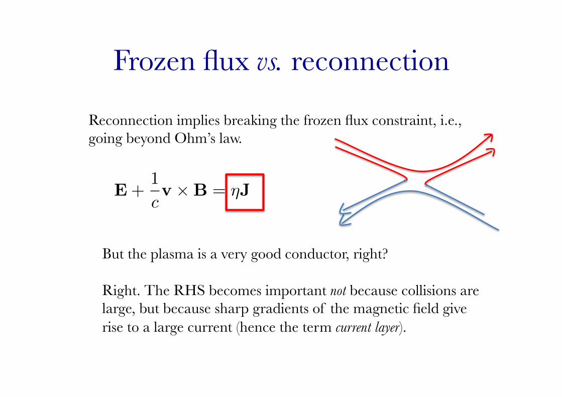
Reconnection implies breaking the frozen flux constraint, i.e., going beyond Ohm’s law.

E+1

cv ×B = ηJ

But the plasma is a very good conductor, right?

Frozen flux vs. reconnection

Reconnection implies breaking the frozen flux constraint, i.e., going beyond Ohm’s law.

E+1

cv ×B = ηJ

But the plasma is a very good conductor, right?

Right. The RHS becomes important not because collisions are large, but because sharp gradients of the magnetic field give rise to a large current (hence the term current layer).

ONE WAY TO GET RECONNECTION GOING: THE TEARING MODE

The tearing instability �[Furth, Killeen & Rosenbluth (FKR) ‘63; Coppi et al. ’76]

(Fitzpatrick’s book)

Take MHD eqs:

∂B

∂t= ∇× (v ×B) + η∇2B

ρdv

dt= −∇p+

1

cJ×B

Linearise (assume ): ∇ · v = 0

B0 = B0yf(x)y; v0 = 0

γBx = ikB0yf(x)vx + η

�d2

dx2− k2

�Bx

γ

�d2

dx2− k2

�vx = ikB0yf(x)

�d2

dx2− k2 − f ��(x)

f(x)

�Bx

Tearing cont’d

Definitions: τH = 1/kB0y; τη = a2/η

v = z×∇φ; B = z×∇ψ

Normalize lengths: x/a → x; ka → k

iφ/γτH → φRescale (for convenience):

ψ − f(x)φ =1

γτη

�d2

dx2− k2

�ψ

γ2τ2Hφ = −f(x)

�d2

dx2− k2 − f ��(x)

f(x)

�

Tearing cont’d

Ordering: 1/τη � γ � 1/τHExpect growth rate to be intermediate between resistive diffusion (very slow) and ideal MHD (very fast)

ψ − f(x)φ =1

γτη

�d2

dx2− k2

�ψ

γ2τ2Hφ = −f(x)

�d2

dx2− k2 − f ��(x)

f(x)

�ψ

Tearing cont’d

Ordering: 1/τη � γ � 1/τHExpect growth rate to be intermediate between resistive diffusion (very slow) and ideal MHD (very fast)

It’s a reconnecting mode: expect ideal MHD to be valid away from the reconnection layer (outer region), and resistive effects to be important in the reconnection layer (inner region = boundary layer)

ψ − f(x)φ =1

γτη

�d2

dx2− k2

�ψ

γ2τ2Hφ = −f(x)

�d2

dx2− k2 − f ��(x)

f(x)

�ψ

Tearing cont’d

Outer region:

Overlap region:

φ =ψ

f(x); f(x)

�d2

dx2− k2

�ψ = f ��(x)ψ

x � 1 → f(x) ≈ x ⇒ ψ�� = 0

For a reconnecting mode, ψ(0) must be finite. Need even solution.

ψ ≈ ψ0 + |x|ψ�0

This solution is discontinuous at x=0. A measure of that discontinuity is the instability parameter:

∆� =

�d

dxlnψ

�0+

0−

=2ψ�

0

ψ0

Tearing cont’d

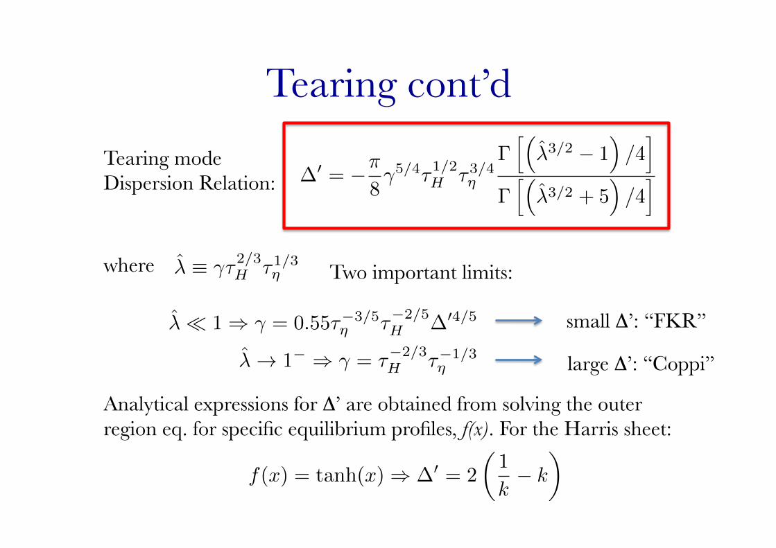
Tearing mode Dispersion Relation: ∆� = −π

8γ5/4τ1/2

Hτ3/4η

Γ��

λ3/2 − 1�/4

�

Γ��

λ3/2 + 5�/4

�

where λ ≡ γτ2/3H

τ1/3η

λ � 1 ⇒ γ = 0.55τ−3/5η τ−2/5

H∆�4/5

λ → 1− ⇒ γ = τ−2/3H

τ−1/3η

Two important limits:

small Δ’: “FKR”

large Δ’: “Coppi”

Analytical expressions for Δ’ are obtained from solving the outer region eq. for specific equilibrium profiles, f(x). For the Harris sheet:

f(x) = tanh(x) ⇒ ∆� = 2

�1

k− k

�

NONLINEAR RECONNECTION: THE SWEET-PARKER MODEL

The simplest description of reconnection: the Sweet-Parker model

δSP

LCS

Peter Sweet (‘58) and Eugene Parker (‘57) attempted to describe reconnection within the framework of resistive magnetohydrodynamics (MHD).


δSP

LCS

S = LCSVA/η

δSP /LCS ∼ S−1/2

uin/VA ∼ S−1/2

E ∼ cB0VAS−1/2



δSP

LCS

S = LCSVA/η

δSP /LCS ∼ S−1/2

uin/VA ∼ S−1/2

E ∼ cB0VAS−1/2


Typical solar corona parameters yield S~1014 ; this theory then predicts that flares should last ~2 months; in fact, flares last 15min – 1h. (still, Sweet-Parker (SP) theory was a great improvement on simple resistive diffusion of magnetic fields, which would yield ~3.106 years…)

Does the Sweet-Parker model work?

Sure!

Does the Sweet-Parker model work?

Sure!

Hmm… maybe it doesn’t…

Loureiro et al. ‘05

BEYOND SWEET-PARKER: TEARING INSTABILITY OF THE

CURRENT SHEET

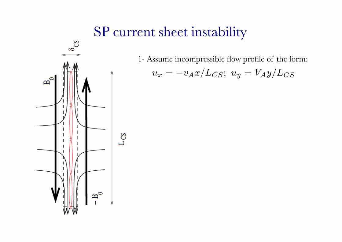
SP current sheet instability

1- Assume incompressible flow profile of the form:

ux = −vAx/LCS ; uy = VAy/LCS



2- Obtain consistent reconnecting magnetic field from resistive induction equation.





3- Linearize RMHD eqs and look for perturbations


γ � VA/LCS ≡ 1/τA





4- Asymptotic expansion using S>>1.








5- Obtain:



γmaxτA ∼ S1/4

kmaxLCS ∼ S3/8






5- Obtain:



γmaxτA ∼ S1/4

kmaxLCS ∼ S3/8

Super Alfvenic growth!!

Plasmoids galore!!

(Loureiro et al. ’07, ‘13)

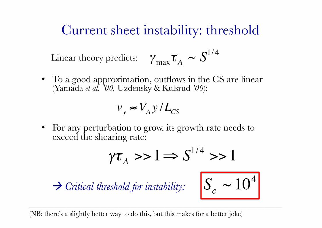
Current sheet instability: threshold

•  To a good approximation, outflows in the CS are linear (Yamada et al. ’00, Uzdensky & Kulsrud ’00):

•  For any perturbation to grow, its growth rate needs to exceed the shearing rate:

€

vy ≈VA y /LCS

€

γτA >>1⇒ S1/ 4 >>1

Critical threshold for instability:

€

Sc ~ 104

€

γmaxτA ~ S1/ 4

Linear theory predicts:

_______________________________________________________________________ (NB: there’s a slightly better way to do this, but this makes for a better joke)

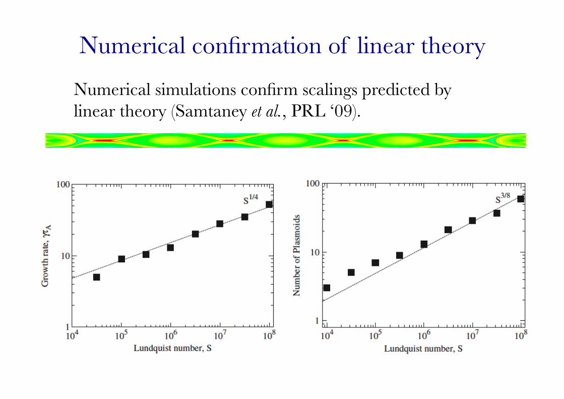
Numerical confirmation of linear theory

Numerical simulations confirm scalings predicted by linear theory (Samtaney et al., PRL ‘09).

Nonlinear stage: �hierarchical plasmoid chains

(Shibata & Tanuma ’01)

Long current sheets (S > Sc ~ 104) are violently unstable to multiple plasmoid formation.

•  Current layers between any two plasmoids are themselves unstable to the same instability if

•  Plasmoid hierarchy ends at the critical layer:

•  N ~ L / Lc plasmoids separated by near-critical current sheets.

Sn = LnVA/η > Sc

Hierarchical Plasmoid Chains

(Shibata & Tanuma ’01)

Long current sheets (S > Sc ~ 104) are violently unstable to multiple plasmoid formation.

Barta et al., ‘11 (also Huang et al., ‘10)

Plasmoid-dominated reconnection: �the ULS model

Theoretical model (ULS) (Uzdensky et al., PRL ’10) attempts to describe reconnection in stochastic plasmoid chains.

Key results: •  Nonlinear statistical steady state exists; effective reconnection

rate is: Eeff ~ Sc

-1/2~ 0.01 independent of S !

•  Plasmoid flux and size distribution functions are: f(ψ) ~ ψ-2 ; f(wx) ~ wx

-2

•  Monster plasmoids form occasionally: wmax ~ 0.1 L --- can disrupt the chain, observable

High-Lundquist-number reconnection Direct numerical simulations to investigate magnetic reconnection at S>Sc (Loureiro et al., PoP ‘12)

S=106, res. 163842

(see also Huang and Bhattacharjee ‘12,’13)

Reconnection and dissipation rates

Eeff ≈ 0.02

~ 40% of incoming magnetic energy dissipated into heat

Sweet-Parker rate

Sweet-Parker model breaks down for S>104

(see also: Lapenta ‘08, Bhattacharjee ‘09, Huang ‘10, ‘12) (Loureiro et al., ‘12)

Monster plasmoid formation tim

e

Monster plasmoid formation

Time-to-monster a few Alfvén times, independent of S

(Loureiro et al., ‘12)

Monster plasmoids: application to blazar flares?

Minute-timescale TeV flares appear to be a generic feature of blazar activity. Recent model proposed by Giannios (arXiv:1211.0296) claims that envelope can be do the reconnection, while the “bursts” could be due to monster plasmoids.

Reality check

There seems to be abundant evidence for plasmoids in solar flares and Earth’s magnetotail (see Loureiro PRE ‘13 and refs. therein).

Karlicky & Kliem ‘10

Reality check

Takasao et al. ‘12

RECONNECTION IN A TURBULENT PLASMA

Reconnection in a turbulent background

Many (if not all) environments where reconnection occurs are turbulent – how does that affect reconnection?

Lazarian & Vishniac ‘99

Very roughly: it’s SP but now the width d is determined by the typical field line wandering:

uinL = VA∆x

More precisely:

uin =λ⊥λ�

L

λ�VA

Plug in your favourite turbulence model (e.g., GS95: ) Independent of η.

λ� ∼ λ2/3⊥


No background turbulence

With background turbulence

Kowal et al. ‘09 S = 103


Kowal et al., ‘09

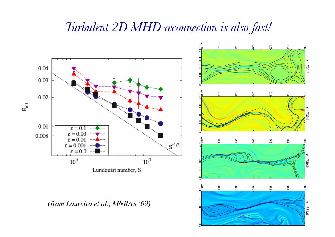
Turbulent 2D MHD reconnection is also fast!

(from Loureiro et al., MNRAS ‘09)

KINETIC RECONNECTION

Enter kinetics

What happens if

δSP < ρi, c/ωpi

Alternatively, even if , one is almost certain to get: δSP > ρi, c/ωpi

δc < ρi, c/ωpi

ρi

??

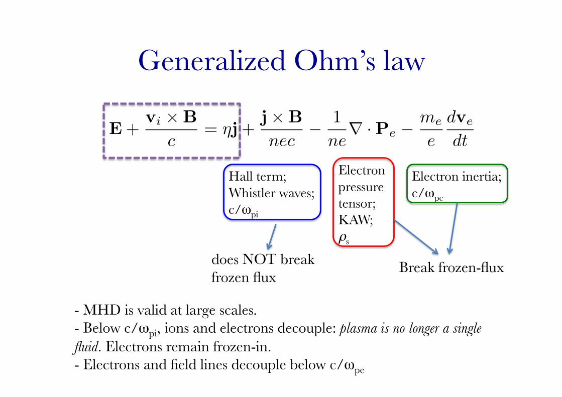
Generalized Ohm’s law

E+vi ×B

c= ηj


Hall term; Whistler waves; c/ωpi

E+vi ×B

c= ηj+

j×B

nec



Electron pressure tensor; KAW; ρs

E+vi ×B

c= ηj+

j×B

nec− 1

ne∇ ·Pe




Electron inertia; c/ωpe

E+vi ×B

c= ηj+

j×B

nec− 1

ne∇ ·Pe −

me

e

dve

dt





Break frozen-flux does NOT break frozen flux

E+vi ×B

c= ηj+

j×B

nec− 1

ne∇ ·Pe −

me

e

dve

dt





Break frozen-flux does NOT break frozen flux

E+vi ×B

c= ηj+

j×B

nec− 1

ne∇ ·Pe −

me

e

dve

dt

- MHD is valid at large scales. - Below c/ωpi, ions and electrons decouple: plasma is no longer a single fluid. Electrons remain frozen-in. - Electrons and field lines decouple below c/ωpe

GEM challenge

GEM challenge, Birn et al. ‘01

What is the minimal plasma description that yields fast reconnection rates?

The signature of Hall reconnection: quadrupolar magnetic field

(Breslau & Jardin ’03)

[Also observed in MRX (see H. Ji’s talk)]

Physical explanation of quadrupole field: Uzdensky & Kulsrud ‘06

Kinetic means kinetic…

Numata et al. ‘11

Two-fluid tearing mode theories seem to fail to predict linear tearing mode growth rates. The reason is the failure of simple equations of state (e.g., isothermal closure is not valid).

Kinetic means kinetic…

Numata et al. ‘11

Strongly suggests that minimum model for weakly collisional reconnection may be kinetic ions + drift kinetic electrons (and even that may not be sufficient)

Connection with other topics at this school

Reconnection in accretion disks (Hawley & Balbus ‘92)

Firehose / mirror in high-β reconnection (Schoeffler ‘11)

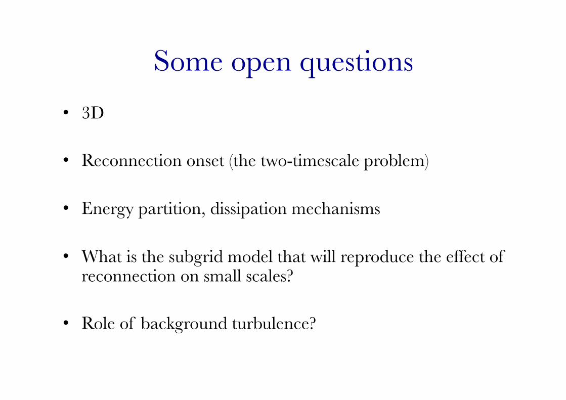
Some open questions

•  3D

•  Reconnection onset (the two-timescale problem)

•  Energy partition, dissipation mechanisms

•  What is the subgrid model that will reproduce the effect of reconnection on small scales?

•  Role of background turbulence?

Bibliography Selected references for topics covered or (mentioned) in this talk (this list is NOT exhaustive; many important papers NOT here)

•  General: –  Books by D. Biskamp and Priest & Forbes –  Recent review papers: Zweibel & Yamada ‘09, Yamada et al., ’10 –  Tutorial: Kulsrud ‘01

•  Tearing mode (fluid): –  MHD: Furth et al. ‘63, Coppi ’75 –  Collisionless: Cowley ’86, Porcelli ’91 (v. good overview in App. B of Zocco & Schekochihin ‘11) –  Rutherford ’73; Waelbroeck ’93 (nonlinear stage) –  Militello & Porcelli ’04, Escande & Ottaviani ‘04 “POEM”, saturation –  Steinolfson & Van Hoven ‘84, Loureiro et al. ’05 (sims.)

•  Tearing mode (kinetic): –  Coppi ’65, Drake & Lee ’77, Cowley ’86, Porcelli ‘91, Numata ‘11 (see App. B of Zocco &

Schekochihin ‘11)

•  Forced Reconnection: –  Hahm & Kulsrud ’84, Fitzpatrick ‘03, Cole & Fitzpatrick ’04

Bibliography cont’d •  Sweet-Parker:

–  Parker ‘57, Sweet ’58 –  Biskamp ‘86, Uzdensky ’00

•  Petschek ’64

•  Plasmoids: –  Shibata & Tanuma ‘01, Loureiro et al. ’07,’12,’13, Lapenta ‘08, Bhattacharjee ‘09, Daughton ‘09, Cassak ‘09,

Samtaney ‘09, Huang ’10, ’12, ‘13, Uzdensky ‘10, Barta ‘08,’11, etc

•  Reconnection in a turbulent plasma: –  Matthaeus & Lamkin ‘86, Lazarian & Vishniac ’99, Kowal ‘09, Loureiro ’09, Karimabadi ’13

•  Trigger: Bhattacharjee ‘04, Katz et al. ’10

•  Reconnection experiments: see H. Ji’s talk; Egedal; Brown, etc.

•  Reconnection simulations: see R. Grauer’s talk

_________________________________________________________ Acknowledgements: Research funded by FCT grant no. PTDC118187

n. f. loureiro - ompuserpages.irap.omp.eu/~frincon/houches/loureiro.pdf · an introduction to...

Documents