NBER WORKING PAPER SERIES

INTERNATIONAL CAPITAL FLOWS AND HOUSE PRICES:THEORY AND EVIDENCE

Jack FavilukisDavid Kohn

Sydney C. LudvigsonStijn Van Nieuwerburgh

Working Paper 17751http://www.nber.org/papers/w17751

NATIONAL BUREAU OF ECONOMIC RESEARCH1050 Massachusetts Avenue

Cambridge, MA 02138January 2012

Prepared for the National Bureau of Economic Research Housing and the Financial Crisis Conference,November 17-18, 2011, Cambridge, MA. We are grateful to John Driscoll, Victoria Ivashina, StevenLaufer, and Nikolai Roussanov for helpful comments and to Atif Mian and Amir Sufi for data. Thismaterial is based on work supported by the National Science Foundation under Grant No. 1022915to Ludvigson and Van Nieuwerburgh. The views expressed herein are those of the authors and donot necessarily reflect the views of the National Bureau of Economic Research.

NBER working papers are circulated for discussion and comment purposes. They have not been peer-reviewed or been subject to the review by the NBER Board of Directors that accompanies officialNBER publications.

© 2012 by Jack Favilukis, David Kohn, Sydney C. Ludvigson, and Stijn Van Nieuwerburgh. All rightsreserved. Short sections of text, not to exceed two paragraphs, may be quoted without explicit permissionprovided that full credit, including © notice, is given to the source.

International Capital Flows and House Prices: Theory and EvidenceJack Favilukis, David Kohn, Sydney C. Ludvigson, and Stijn Van NieuwerburghNBER Working Paper No. 17751January 2012JEL No. F20,F32,G12,G21

ABSTRACT

The last fifteen years have been marked by a dramatic boom-bust cycle in real estate prices, accompaniedby economically large fluctuations in international capital flows. We argue that changes in internationalcapital flows played, at most, a small role in driving house price movements in this episode and that,instead, the key causal factor was a financial market liberalization and its subsequent reversal. Usingobservations on credit standards, capital flows, and interest rates, we find that a bank survey measureof credit supply, by itself, explains 53 percent of the quarterly variation in house price growth in theU.S. over the period 1992-2010, while it explains 66 percent over the period since 2000. By contrast,once we control for credit supply, various measures of capital flows, real interest rates, and aggregateactivity—collectively—add less than 5% to the fraction of variation explained for these same movementsin home values. Credit supply retains its strong marginal explanatory power for house price movementsover the period 2002-2010 in a panel of international data, while capital flows have no explanatorypower.

Jack FavilukisLondon School of EconomicsDepartment of FinanceHoughton Street, London WC2A 2AEUnited Kingdomjack.favilukis@gmail.com

David KohnDepartment of EconomicsNew York University19 W. 4th Street 6th FloorNew York, NY 10012dk1310@nyu.edu

Sydney C. LudvigsonDepartment of EconomicsNew York University19 W. 4th Street, 6th FloorNew York, NY 10002and NBERsydney.ludvigson@nyu.edu

Stijn Van NieuwerburghStern School of BusinessNew York University44 W 4th Street, Suite 9-120New York, NY 10012and NBERsvnieuwe@stern.nyu.edu

1 Introduction

The last fifteen years have been marked by a dramatic boom-bust cycle in real estate prices, a

pattern unprecedented both in amplitude and in scope that affected many countries around the

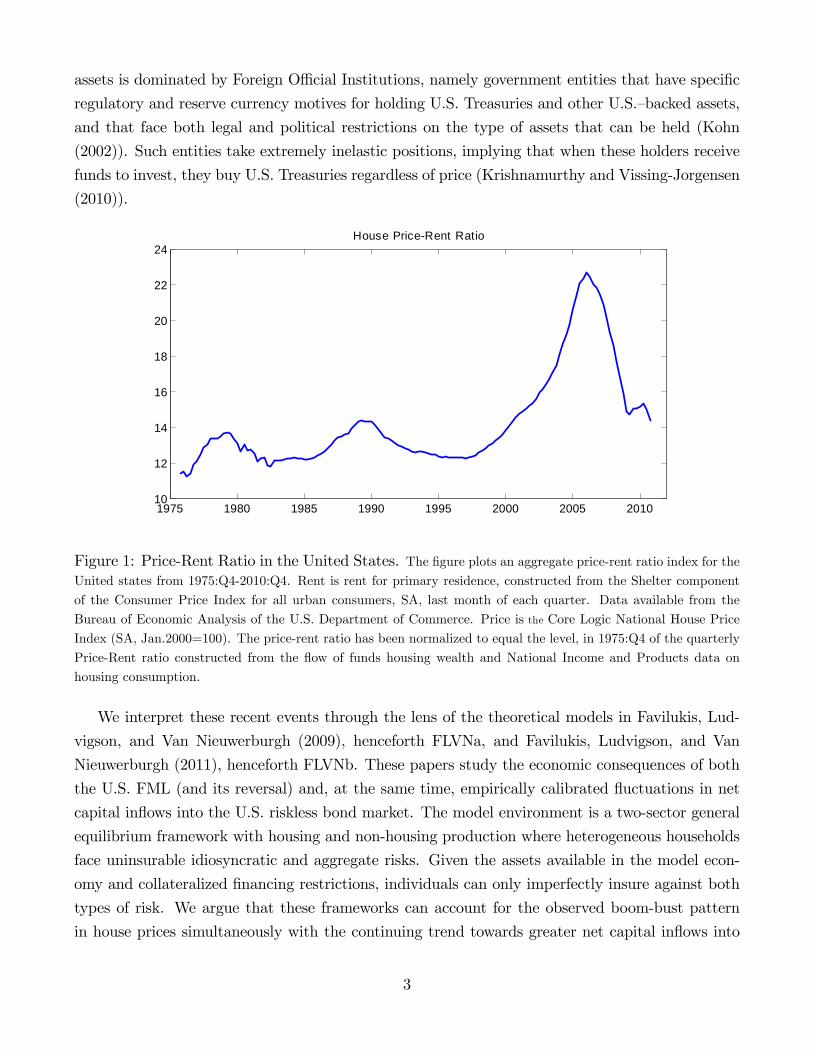
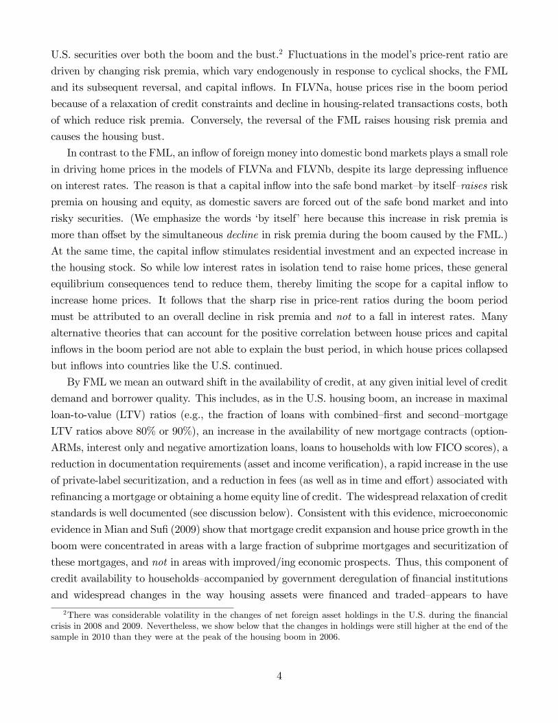
globe and most regions within the United States (Figure 1). Over the same period, there were

economically large fluctuations in international capital flows. Countries that exhibited the largest

house price increases also often exhibited large and increasing net inflows of foreign capital that

bankrolled sharply higher trade deficits. Economists have debated the role of international capital

flows in explaining these movements in house prices and asset market volatility more generally. A

common hypothesis is that house price increases are positively related to a rise in the country’s

net foreign inflows, either because they directly cause house price increases (perhaps by lowering

real interest rates), or because other factors simultaneously drive up both house prices and capital

inflows. In this article, we study both theory and evidence that bears on this hypothesis, focusing

on the unprecedented boom-bust cycle in housing markets that took place over the last 15 years.

We argue that changes in international capital flows played, at most, a small role driving house

price movements in this episode and that, instead, the key causal factor was a financial market

liberalization and its subsequent reversal that took place in many countries largely independently

of international capital flows. Financial market liberalization (FML hereafter) refers to a set of

regulatory and market changes and subsequent decisions by financial intermediaries that made it

easier and less costly for households to obtain mortgages, borrow against home equity, and adjust

their consumption.

By contrast, we argue that net capital flows into the United States over both the boom and

the bust period in housing have followed a largely independent path, driven to great extent by

foreign governments’ regulatory, reserve currency, and economic policy motives. Consider the

value of foreign holdings of U.S. assets minus U.S. holdings of foreign assets, referred to hereafter

as net foreign asset holdings in the U.S., or alternatively, as the U.S. net liability position. A

positive change in net foreign asset holdings indicates a capital inflow, or more borrowing from

abroad.1 As we show below, from 1994 to 2010, only the change in net foreign holdings of U.S.

securities (equities, corporate, U.S. Agency and Treasury bills and bonds) show any discernible

upward trend. Moreover, among securities, the upward trend has been driven almost entirely by

an increase in net foreign holdings of U.S. assets considered to be safe stores-of-value, specifically

U.S. Treasury and Agency debt. Yet inflows into these securities, rather than declining during the

housing bust, have on average continued to increase. Importantly, foreign demand for U.S. “safe”

1What we have defined as net foreign asset holdings, or the U.S. net liability position, is equal to the negative ofthe U.S. net international investment position in the U.S. Bureau of Economic Analysis balance of payments system.A country’s resource constraint limits its expenditures on (government and private) consumption and investmentgoods, fees, and services, to its domestic output plus the change in the market value of its net liabilities (minus thechange in the net international investment position). Thus a country’s ability to spend in excess of domestic incomein a given period depends positively on the change in its net foreign liabilities.

2

assets is dominated by Foreign Offi cial Institutions, namely government entities that have specific

regulatory and reserve currency motives for holding U.S. Treasuries and other U.S.—backed assets,

and that face both legal and political restrictions on the type of assets that can be held (Kohn

(2002)). Such entities take extremely inelastic positions, implying that when these holders receive

funds to invest, they buy U.S. Treasuries regardless of price (Krishnamurthy and Vissing-Jorgensen

(2010)).

1975 1980 1985 1990 1995 2000 2005 201010

12

14

16

18

20

22

24House Price­Rent Ratio

Figure 1: Price-Rent Ratio in the United States. The figure plots an aggregate price-rent ratio index for theUnited states from 1975:Q4-2010:Q4. Rent is rent for primary residence, constructed from the Shelter component

of the Consumer Price Index for all urban consumers, SA, last month of each quarter. Data available from the

Bureau of Economic Analysis of the U.S. Department of Commerce. Price is the Core Logic National House Price

Index (SA, Jan.2000=100). The price-rent ratio has been normalized to equal the level, in 1975:Q4 of the quarterly

Price-Rent ratio constructed from the flow of funds housing wealth and National Income and Products data on

housing consumption.

We interpret these recent events through the lens of the theoretical models in Favilukis, Lud-

vigson, and Van Nieuwerburgh (2009), henceforth FLVNa, and Favilukis, Ludvigson, and Van

Nieuwerburgh (2011), henceforth FLVNb. These papers study the economic consequences of both

the U.S. FML (and its reversal) and, at the same time, empirically calibrated fluctuations in net

capital inflows into the U.S. riskless bond market. The model environment is a two-sector general

equilibrium framework with housing and non-housing production where heterogeneous households

face uninsurable idiosyncratic and aggregate risks. Given the assets available in the model econ-

omy and collateralized financing restrictions, individuals can only imperfectly insure against both

types of risk. We argue that these frameworks can account for the observed boom-bust pattern

in house prices simultaneously with the continuing trend towards greater net capital inflows into

3

U.S. securities over both the boom and the bust.2 Fluctuations in the model’s price-rent ratio are

driven by changing risk premia, which vary endogenously in response to cyclical shocks, the FML

and its subsequent reversal, and capital inflows. In FLVNa, house prices rise in the boom period

because of a relaxation of credit constraints and decline in housing-related transactions costs, both

of which reduce risk premia. Conversely, the reversal of the FML raises housing risk premia and

causes the housing bust.

In contrast to the FML, an inflow of foreign money into domestic bond markets plays a small role

in driving home prices in the models of FLVNa and FLVNb, despite its large depressing influence

on interest rates. The reason is that a capital inflow into the safe bond market—by itself—raises risk

premia on housing and equity, as domestic savers are forced out of the safe bond market and into

risky securities. (We emphasize the words ‘by itself’here because this increase in risk premia is

more than offset by the simultaneous decline in risk premia during the boom caused by the FML.)

At the same time, the capital inflow stimulates residential investment and an expected increase in

the housing stock. So while low interest rates in isolation tend to raise home prices, these general

equilibrium consequences tend to reduce them, thereby limiting the scope for a capital inflow to

increase home prices. It follows that the sharp rise in price-rent ratios during the boom period

must be attributed to an overall decline in risk premia and not to a fall in interest rates. Many

alternative theories that can account for the positive correlation between house prices and capital

inflows in the boom period are not able to explain the bust period, in which house prices collapsed

but inflows into countries like the U.S. continued.

By FML we mean an outward shift in the availability of credit, at any given initial level of credit

demand and borrower quality. This includes, as in the U.S. housing boom, an increase in maximal

loan-to-value (LTV) ratios (e.g., the fraction of loans with combined—first and second—mortgage

LTV ratios above 80% or 90%), an increase in the availability of new mortgage contracts (option-

ARMs, interest only and negative amortization loans, loans to households with low FICO scores), a

reduction in documentation requirements (asset and income verification), a rapid increase in the use

of private-label securitization, and a reduction in fees (as well as in time and effort) associated with

refinancing a mortgage or obtaining a home equity line of credit. The widespread relaxation of credit

standards is well documented (see discussion below). Consistent with this evidence, microeconomic

evidence in Mian and Sufi(2009) show that mortgage credit expansion and house price growth in the

boom were concentrated in areas with a large fraction of subprime mortgages and securitization of

these mortgages, and not in areas with improved/ing economic prospects. Thus, this component of

credit availability to households—accompanied by government deregulation of financial institutions

and widespread changes in the way housing assets were financed and traded—appears to have

2There was considerable volatility in the changes of net foreign asset holdings in the U.S. during the financialcrisis in 2008 and 2009. Nevertheless, we show below that the changes in holdings were still higher at the end of thesample in 2010 than they were at the peak of the housing boom in 2006.

4

fluctuated, to great extent, independently of current and future economic conditions.

But credit availability can also change endogenously in response to fluctuations in the aggregate

economy and to revisions in expectations about future economic conditions, including house price

growth. This information is reflected immediately in collateral values that constrain borrowing

capacity. As in classic financial accelerator models (e.g., Bernanke and Gertler (1989), Kiyotaki

and Moore (1997)), endogenous shifts in borrowing capacity imply that economic shocks have a

much larger effect on asset prices than they would in frictionless environments without collater-

alized financing restrictions. Both exogenous and endogenous components of time-varying credit

availability to households are operative in the model of FLVNa.

While endogenous fluctuations in credit availability are clearly important in theory, it is unclear

how quantitatively important they have been empirically, especially in the recent housing boom-

bust episode. Some researchers have argued that credit availability is primarily driven by the

political economy, and in particular by political constituencies that influence bank regulation related

to credit availability (e.g., Mian, Sufi, and Trebbi (2009); Rice and Strahan (2010); Boz and

Mendoza (2011); Rajan and Ramcharan (2011b)). Such a component to credit availability could

in fact be independent of economic fundamentals, expectations of future fundamentals, and credit

demand.

Using observations on credit standards, capital flows, and interest rates for the U.S. and for a

panel of 11 countries, we present evidence on how these variables are related to real house price

movements in recent data. Our main measure of credit standards is compiled from quarterly bank

surveys of senior loan offi cers, carried out by national central banks as part of their regulatory

oversight. We consider this a summary indicator of fluctuations in the variables associated with a

FML, as described above. The surveys specifically address changes in a bank’s supply of credit, as

distinct from changes in its perceived demand for credit. We find for the U.S. that this measure of

credit supply, by itself, explains 53 percent of the quarterly variation in house price growth over the

period 1992-2010, while it explains 66 percent over the period since 2000. By contrast, controlling

for credit supply, various measures of capital flows, real interest rates, and aggregate activity—

collectively—add less than 5% to the fraction of variation explained for these same movements

in home values. Credit supply retains its strong marginal explanatory power for house price

movements over the period 2002-2010 in a panel of international data, while capital flows have

no explanatory power. Moreover, credit standards continues to be the most important variable

related to future home price fluctuations even when it has been rendered statistically orthogonal

to banks’perceptions of credit demand, and even when controlling for expected future economic

growth and expected future real interest rates. Taken together, these findings suggest that a stark

shift in bank lending practices—conspicuous in the FML and its reversal—were at the root of the

housing crisis.

The rest of this paper is organized as follows. The next section discusses theoretical literature

5

that has addressed the link between house prices, capital flows and/or credit supply. To provide

a theoretical frame of reference, here we also describe in detail the predictions of FLVNa for

house price movements. Section 3 turns to the data, presenting stylized facts on international

capital flows, interest rates and credit standards. Section 4 presents an empirical analysis of

the linkage between capital flows and house price fluctuations, controlling for measures of credit

supply, economic activity, and real interest rates. Section 5 concludes. Section 6 is an Appendix

that provides details on the data we use and on our estimation methodology.

2 Theories

A number of studies have addressed the link between house prices and capital flows, focusing on

the recent boom period in housing. For brevity, we will refer to the period of rapid home price

appreciation from 2000 to 2006 as the boom period in the U.S., and the period 2007 to present as

the bust.

The global savings glut hypothesis (Bernanke (2005), Mendoza, Quadrini, and Rios-Rull (2007),

Bernanke (2008), Caballero, Fahri, and Gourinchas (2008), Caballero and Krishnamurthy (2009))

contends that the excess savings of developing countries, notably China and emerging Asia, sought

safe, high-quality financial assets that their own economies could not provide. Because of the depth,

breadth, and safety of U.S. Treasury and Agency markets, those savings predominantly found their

way to the United States. Some have directly linked these patterns to higher U.S. home prices,

arguing that low interest rates (driven in part by the capital inflow) were a key determinant of

higher house prices during the boom (e.g., Bernanke (2005), Himmelberg, Mayer, and Sinai (2005),

Bernanke (2008), Taylor (2009), Adam, Marcet, and Kuang (2011)). In a similar spirit, Caballero

and Krishnamurthy (2009) identify the start of the housing boom with the Asian financial crisis

which fueled the demand for U.S. risk-free assets. In their model, Asian savers turn to U.S. assets,

resulting in a net capital inflow for the U.S. Global interest rates then fall in their model because

the U.S. economy is presumed to grow more slowly than the rest of the world.

Laibson and Mollerstrom (2010) have criticized the global savings glut hypothesis by noting

that an increase in world-wide savings should have led to an investment boom in countries that

were large importers of capital, notably the U.S. Instead, the U.S. experienced a consumption boom

that accompanied the housing boom, suggesting that saving world-wide was not unusually high.

Laibson and Mollerstrom (2010) present an alternative interpretation of the correlation between

home values and capital flows during the boom based on asset bubbles. Assuming a bubble in the

housing market, they argue that the rise in housing wealth generated by the bubble led to higher

consumption, which in turn led to greater borrowing from abroad and a substantial net capital

inflow to the U.S. A similar idea is presented in Ferrero (2011), but without the bubble. Ferrero

studies a two-sector representative-agent model of international trade in which lower collateral

6

requirements facilitate access to external funding and drive up house prices.

Others have argued that preference shocks and a desire for smooth (across goods) consumption

can generate a correlation between house prices and capital inflows. Gete (2010) shows that

consumption smoothing across tradeable (non-housing) goods and nontradable (housing) goods

can lead to a positive correlation between house prices and current account deficits. With an

exogenous increase in the home country’s preference for housing, productive inputs in the home

country are reallocated toward housing production, so that housing consumption can rise. But

with a preference for smooth consumption across goods, the tradeable non-housing good (presumed

identical across countries) will then be imported from abroad, leading to capital inflows to the home

country.

The theories above fall into two broad categories: those that rely on higher domestic demand

to drive both house prices and capital inflows in the same direction (Gete (2010), Laibson and

Mollerstrom (2010), Ferrero (2011)), and those that rely on capital inflow-driven low interest rates

to drive up house prices (Bernanke (2005), Himmelberg, Mayer, and Sinai (2005), Bernanke (2008),

Taylor (2009), Caballero and Krishnamurthy (2009), Adam, Marcet, and Kuang (2011)). While

these papers were motivated by observations on housing and capital flows during the housing boom,

they also have implications for the housing bust. The former imply that the housing bust should be

associated with a reversal of domestic demand, leading to a capital outflow. The latter imply that

the housing bust should be associated with a rise in real interest rates, correlated with a capital

outflow.

As we show below, recent data pose a number of challenges to these theories. First, while it

is true that real interest rates were low throughout the boom period, they have remained low and

even fallen further in the bust period. Second, while capital certainly flowed into countries like the

U.S. during the boom period, there is no evidence of a clear reversal in this trend during the bust

period.3 These observations suggest that the economic and political forces responsible for driving

capital flows and house prices over the entire period were, to a large extent, distinct. Below we

present empirical evidence that neither capital inflows nor real interest rates bear a strong relation

to house prices in a sample that includes both the boom and the bust.

We interpret these recent events through the lens of the theoretical models in FLVNa and

FLVNb, focusing specifically on the model in FLVNa in which a FML and its reversal are studied.

Rather than reproducing the mathematical description of the model here, we simply describe it

verbally and refer the reader to the original papers for details. Our focus here is on empirical

evidence relating home prices to various indicators as a means of distinguishing among theories.

Next we describe the model in FLVNa, and explain how it differs from the theories above.

3Some empirical studies document a positive correlation between house prices and capital inflows to the U.S.,but these studies typically have data samples that terminate at the end of the boom or shortly thereafter (e.g.,Aizenman and Jinjarak (2009), Kole and Martin (2009)).

7

2.1 The Housing Boom-Bust: A Theory of Time-Varying Risk-Premia

FLVNa study a two-sector general equilibrium model of housing and non-housing production where

heterogenous households face limited risk-sharing opportunities as a result of incomplete financial

markets. A house in the model is a residential durable asset that provides utility to the household, is

illiquid (expensive to trade), and can be used as collateral in debt obligations. The model economy

is populated by a large number of overlapping generations of households who receive utility from

both housing and nonhousing consumption and who face a stochastic life-cycle earnings profile.

We introduce market incompleteness by modeling heterogeneous agents who face idiosyncratic

and aggregate risks against which they cannot perfectly insure, and by imposing collateralized

borrowing constraints on households.

Within the context of this model, FLVNa focus on the macroeconomic consequences of three

systemic changes in housing finance, with an emphasis on how these factors affect risk premia

in housing markets, and how risk premia in turn affect home prices. First, FLVNa investigate

the impact of changes in housing collateral requirements.4 Second, they investigate the impact of

changes in housing transactions costs. Taken together, these two factors represent the theoretical

counterpart to the real-world FML discussed above. Third, FLVNa investigate the impact of an in-

flux of foreign capital into the domestic bond market. FLVNa argue that all three factors fluctuate

over time and changed markedly during and preceding the period of rapid home price appreciation

from 2000-2006, and the subsequent bust. In particular, the boom period was marked by a wide-

spread relaxation of collateralized borrowing constraints and declining housing transactions costs

(including costs associated with mortgage borrowing, home equity extraction, and refinance). The

period was also marked by a sustained depression of long-term interest rates that coincided with a

vast inflow of capital into U.S. safe bond markets. In the aftermath of the credit crisis that began

in 2007, the erosion in credit standards and transactions costs has been sharply reversed.5 We

provide evidence on this below.

The main impetus for rising price-rent ratios in the model in the boom period is the simultaneous

occurrence of positive economic shocks and a financial market liberalization, phenomena that

generate an endogenous decline in risk premia on housing and equity assets. As risk premia fall,

the aggregate house price index relative to aggregate rent, rises. A FML reduces risk premia for

two reasons, both of which are related to the ability of heterogeneous households to insure against

aggregate and idiosyncratic risks. First, lower collateral requirements directly increase access to

4Ferrero (2011) also assumes a relaxation of credit constraints to explain the housing boom. A key distinctionbetween his model and FLVNa, however, is that Ferrero studies a two-country representative agent model, so anincrease in borrowing by the domestic agent is only possible with increase in lending from rest of the world, hencea higher current account deficit. By contrast, in FLVNa, borrowing and lending can happen within the domesticeconomy between heterogeneous agents, so housing finance need not be tied to foreign savings. Thus, a reversal ofthe FML in a setting like that of Ferrero’s would necessitate a capital outflow, whereas in FLVNa it does not.

5Streitfeld (2009) argues that, since the credit crisis, borrowing restrictions and credit constraints have becomeeven more stringent than historical norms in the pre-boom period.

8

credit, which acts as a buffer against unexpected income declines. Second, lower transactions costs

reduce the expense of obtaining the collateral required to increase borrowing capacity and provide

insurance. These factors lead to an increase in risk-sharing, or a decrease in the cross-sectional

variance of marginal utility. The housing bust is caused by a reversal of the FML and of the

positive economic shocks and an endogenous decrease in borrowing capacity as collateral values

fall. These factors lead to an accompanying rise in housing risk premia, driving the house price-rent

ratio lower. Almost all of the theories discussed above are silent on the role of housing risk premia

in driving house price fluctuations.6

It is important to note that the rise in price-rent ratios caused by a financial market liberalization

in FLVNa must be attributed to a decline in risk premia and not to a fall in interest rates. Indeed,

the very changes in housing finance that accompany a financial market liberalization drive the

endogenous interest rate up, rather than down. It follows that, if price-rent ratios rise after a

financial market liberalization, it must be because the decline in risk premia more than offsets

the rise in equilibrium interest rates that is attributable to the FML. This aspect of a FML

underscores the importance of accounting properly for the role of foreign capital over the housing

cycle. Without an infusion of foreign capital, any period of looser collateral requirements and

lower housing transactions costs (such as that which characterized the housing boom) would be

accompanied by an increase in equilibrium interest rates, as households endogenously respond to

the improved risk-sharing opportunities afforded by a financial market liberalization by reducing

precautionary saving.

To model capital inflows, FLVNa introduce foreign demand for the domestic riskless bond into

the market clearing condition. This foreign capital inflow is modeled as driven by governmental

holders who inelastically place all of their funds in domestic riskless bonds. Foreign governmental

holders have a perfectly inelastic demand for safe securities and place all of their funds in those

securities, regardless of their price relative to other assets. Below we discuss data on U.S. inter-

national capital flows that supports this specification of the net capital flows in the United States

over the last 15 years.

The model in FLVNa implies that a rise in foreign purchases of domestic bonds, equal in

magnitude to those observed in the data from 2000-2010, leads to a quantitatively large decline in

the equilibrium real interest rate. Were this decline not accompanied by other, general equilibrium,

effects, it would lead to a significant housing boom in the model. But the general equilibrium effects

imply that a capital inflow is unlikely to have a large effect on house prices even if it has a large

effect on interest rates. One reason for this involves the central role of time-varying housing risk

premia. In models where risk premia are held fixed, a decline in the interest rate of this magnitude

would be suffi cient—by itself—to explain the rise in price-rent ratios observed from 2000-2006 under

6An exception is Caballero and Krishnamurthy (2009), but they do not study housing nor the FML and itsreversal.

9

reasonable calibrations. But with time-varying housing risk premia, the result can be quite different.

Foreign purchases of U.S. bonds crowd domestic savers out of the safe bond market, exposing them

to greater systematic risk in equity and housing markets. In response, risk premia on housing and

equity assets rise, substantially offsetting the effect of lower interest rates and limiting the impact

of foreign capital inflows on home prices.

There is a second offsetting general equilibrium effect. Foreign capital inflows also stimulate

residential investment, raising the expected stock of future housing and lowering the expected

future rental growth rate. Like risk premia, these expectations are reflected immediately house

prices (pushing down the national house price-rent ratio), further limiting the impact of foreign

capital inflows on home prices. The net effect of all of these factors is that a large capital inflow

into safe securities has at most a small positive effect on house prices.

It is useful to clarify the two opposing forces simultaneously acting on housing risk premia

in the model of FLVNa. During the housing boom, there is both a FML and a capital inflow.

As explained, the FML lowers risk premia, while foreign purchases of domestic safe assets raise

risk premia. Under the calibration of the model, the decline in risk premia resulting from the

FML during the boom period is far greater than the rise in risk premia resulting from the capital

inflow. On the whole, therefore, risk premia on housing assets fall, and this is the most important

contributing factor to the an increase in price-rent ratios during the boom. During the bust,

modeled as a reversal of the FML but not the capital inflows, risk premia unambiguously rise even

as interest rates remain low. The rise in risk premia drives the decline in house-price rent ratios.

These features of the model represent significant differences from other theories of capital flows

and house prices. They permit the model to explain not just the housing boom, but also the

housing bust, in which house price-rent ratios fell dramatically even though interest rates remained

low and there has been no clear reversal in the trend toward capital inflows into the U.S. bond

market. Moreover, they underscore the importance of distinguishing between interest rate changes

(which are endogenous) and credit supply. In the absence of a capital inflow, an expansion of

credit supply in the form of lower collateral requirements and lower transactions costs should lead,

in equilibrium, to higher interest rates, rather than lower, as households respond to the improved

risk-sharing/insurance opportunities by reducing precautionary saving. Instead we observed low

real interest rates, generated in the model of FLVNa by foreign capital inflows, but the inflows

themselves are not the key factor behind the housing boom-bust.

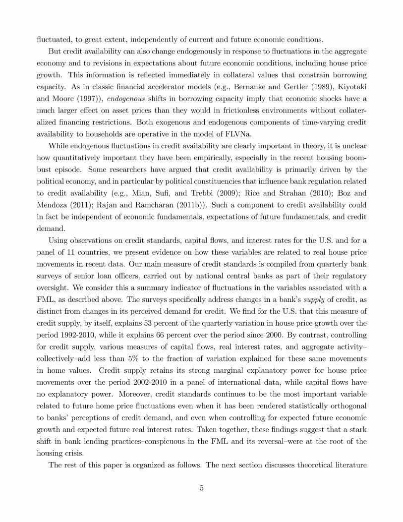
To illustrate the independent role of house prices and capital inflows in the model, Figure 2

plots the transition dynamics for both the aggregate price-rent ratio and for foreign holdings of

domestic assets over the period 2000-2010 from the model of FLVNa. The figure shows the dynamic

behavior of the price-rent ratio in response to a series of shocks designed to mimic both the state

of the economy and housing market conditions over the period 2000-2010. The economy begins

in year 2000 the stochastic steady state of a world with “normal” collateral requirements (i.e.,

10

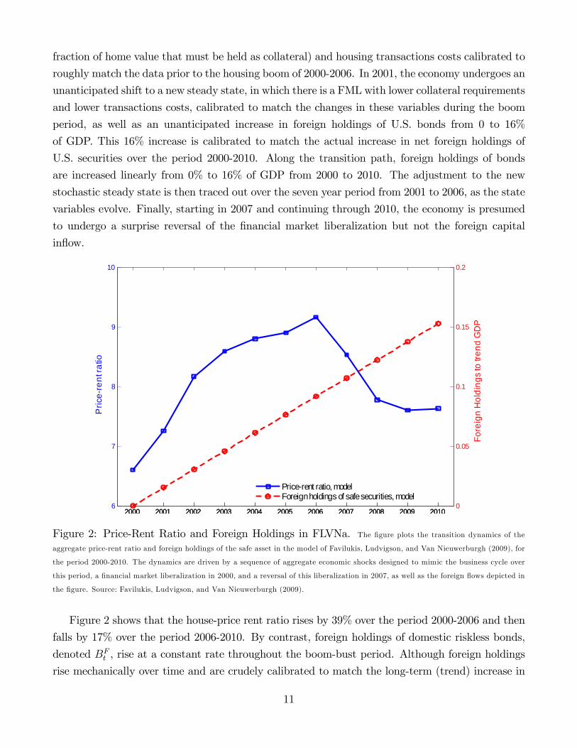
fraction of home value that must be held as collateral) and housing transactions costs calibrated to

roughly match the data prior to the housing boom of 2000-2006. In 2001, the economy undergoes an

unanticipated shift to a new steady state, in which there is a FML with lower collateral requirements

and lower transactions costs, calibrated to match the changes in these variables during the boom

period, as well as an unanticipated increase in foreign holdings of U.S. bonds from 0 to 16%

of GDP. This 16% increase is calibrated to match the actual increase in net foreign holdings of

U.S. securities over the period 2000-2010. Along the transition path, foreign holdings of bonds

are increased linearly from 0% to 16% of GDP from 2000 to 2010. The adjustment to the new

stochastic steady state is then traced out over the seven year period from 2001 to 2006, as the state

variables evolve. Finally, starting in 2007 and continuing through 2010, the economy is presumed

to undergo a surprise reversal of the financial market liberalization but not the foreign capital

inflow.

2000 2001 2002 2003 2004 2005 2006 2007 2008 2009 20106

7

8

9

10

Pric

e­re

nt ra

tio

2000 2001 2002 2003 2004 2005 2006 2007 2008 2009 20100

0.05

0.1

0.15

0.2

Fore

ign 

Hol

ding

s to

 tren

d G

DP

Price­rent ratio, modelForeign holdings of safe securities, model

Figure 2: Price-Rent Ratio and Foreign Holdings in FLVNa. The figure plots the transition dynamics of the

aggregate price-rent ratio and foreign holdings of the safe asset in the model of Favilukis, Ludvigson, and Van Nieuwerburgh (2009), for

the period 2000-2010. The dynamics are driven by a sequence of aggregate economic shocks designed to mimic the business cycle over

this period, a financial market liberalization in 2000, and a reversal of this liberalization in 2007, as well as the foreign flows depicted in

the figure. Source: Favilukis, Ludvigson, and Van Nieuwerburgh (2009).

Figure 2 shows that the house-price rent ratio rises by 39% over the period 2000-2006 and then

falls by 17% over the period 2006-2010. By contrast, foreign holdings of domestic riskless bonds,

denoted BFt , rise at a constant rate throughout the boom-bust period. Although foreign holdings

rise mechanically over time and are crudely calibrated to match the long-term (trend) increase in

11

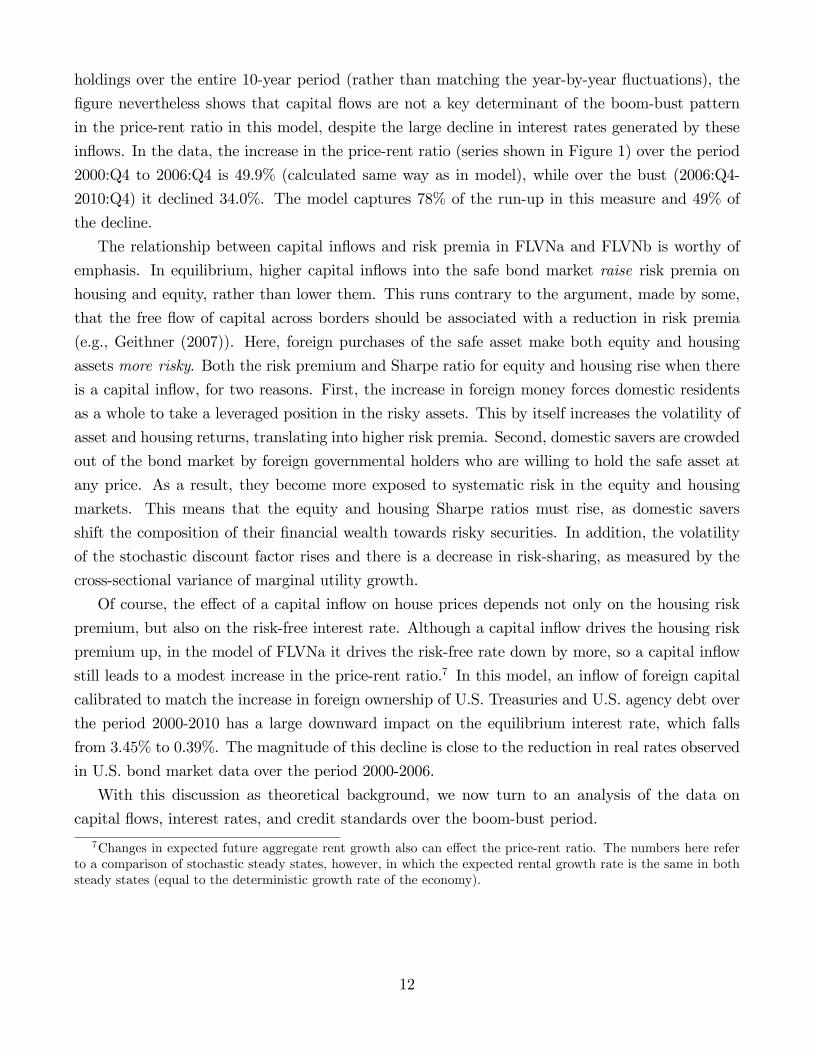
holdings over the entire 10-year period (rather than matching the year-by-year fluctuations), the

figure nevertheless shows that capital flows are not a key determinant of the boom-bust pattern

in the price-rent ratio in this model, despite the large decline in interest rates generated by these

inflows. In the data, the increase in the price-rent ratio (series shown in Figure 1) over the period

2000:Q4 to 2006:Q4 is 49.9% (calculated same way as in model), while over the bust (2006:Q4-

2010:Q4) it declined 34.0%. The model captures 78% of the run-up in this measure and 49% of

the decline.

The relationship between capital inflows and risk premia in FLVNa and FLVNb is worthy of

emphasis. In equilibrium, higher capital inflows into the safe bond market raise risk premia on

housing and equity, rather than lower them. This runs contrary to the argument, made by some,

that the free flow of capital across borders should be associated with a reduction in risk premia

(e.g., Geithner (2007)). Here, foreign purchases of the safe asset make both equity and housing

assets more risky. Both the risk premium and Sharpe ratio for equity and housing rise when there

is a capital inflow, for two reasons. First, the increase in foreign money forces domestic residents

as a whole to take a leveraged position in the risky assets. This by itself increases the volatility of

asset and housing returns, translating into higher risk premia. Second, domestic savers are crowded

out of the bond market by foreign governmental holders who are willing to hold the safe asset at

any price. As a result, they become more exposed to systematic risk in the equity and housing

markets. This means that the equity and housing Sharpe ratios must rise, as domestic savers

shift the composition of their financial wealth towards risky securities. In addition, the volatility

of the stochastic discount factor rises and there is a decrease in risk-sharing, as measured by the

cross-sectional variance of marginal utility growth.

Of course, the effect of a capital inflow on house prices depends not only on the housing risk

premium, but also on the risk-free interest rate. Although a capital inflow drives the housing risk

premium up, in the model of FLVNa it drives the risk-free rate down by more, so a capital inflow

still leads to a modest increase in the price-rent ratio.7 In this model, an inflow of foreign capital

calibrated to match the increase in foreign ownership of U.S. Treasuries and U.S. agency debt over

the period 2000-2010 has a large downward impact on the equilibrium interest rate, which falls

from 3.45% to 0.39%. The magnitude of this decline is close to the reduction in real rates observed

in U.S. bond market data over the period 2000-2006.

With this discussion as theoretical background, we now turn to an analysis of the data on

capital flows, interest rates, and credit standards over the boom-bust period.

7Changes in expected future aggregate rent growth also can effect the price-rent ratio. The numbers here referto a comparison of stochastic steady states, however, in which the expected rental growth rate is the same in bothsteady states (equal to the deterministic growth rate of the economy).

12

3 Trends in Capital Flows, Interest Rates, Credit Supply

While the notion of a global savings glut is controversial, recent data clearly suggest a reallocation

of savings away from the developed world, and toward the developing world, the so-called global

imbalances phenomenon. Unlike any prior period, global financial integration allowed for the

channeling of one country’s excess savings towards another country’s real estate boom. Such

financing occurred directly, for example by German banks’purchases of U.S. subprime securities,

but also indirectly through the U.S. Treasury and Agency bond markets. As the world’s sole

supplier of a global reserve currency, the U.S. experienced a surge in foreign ownership of U.S.

Treasuries and Agency bonds. Agency bonds refers to the debt of the two government-sponsored

enterprises (GSEs) Freddie Mac and Fannie Mae, as well as to the mortgage-backed securities

that they issue and guarantee. Due to their ambivalent private-public structure and their history

as agencies of the federal government, private market investors (including foreign investors) have

always assumed that the debt of Freddie Mac and Fannie Mae was implicitly backed by the U.S.

Treasury. That implicit backing became an explicit backing in September 2008 when Freddie

Mac and Fannie Mae were taken into government conservatorship. See Acharya, Richardson, Van

Nieuwerburgh, and White (2011) for details on the GSEs.

In this section, we discuss in detail data showing the trends in capital flows, U.S. real inter-

est rates, and the relaxation and subsequent tightening of housing credit constraints and credit

standards.

3.1 International Capital Flows

The Treasury International Capital (TIC) reporting system is the offi cial source of U.S. securities

flows data. It reports monthly data (with a six week lag) on foreigners purchases and sales of

all types of financial securities (equities, corporate, Agency, and Treasury bonds). We refer to

these monthly transactions data as the TIC flows data. The TIC system also produces periodic

benchmark surveys of the market value of foreigners’net holdings, or net asset positions, in U.S.

securities. Unlike the flows data, these data take into account the net capital gains on gross foreign

assets and liabilities. We refer to these as the TIC holdings data. The holdings data are collected

in detailed surveys conducted in December of 1978, 1984, 1989, and 1994, in March 2000, and

annually in June from 2002 to 2010. The survey data on holdings is thought to be of higher

quality than the flows data because it more accurately accounts for valuation effects (Warnock and

Warnock (2009)).8

The Bureau of Economic Analysis (BEA) in the U.S. Department of Commerce also provides

8As explained in Warnock and Warnock (2009), reporting to the surveys is mandatory, with penalties for non-compliance, and the data are subjected to extensive analysis and editing. Data on foreign holdings of U.S. securitiesare available at http://www.treasury.gov/resource-center/data-chart-center/tic/Pages/index.aspx.

13

annual estimates of the value of accumulated stocks (holdings) of U.S.-owned assets abroad and of

foreign-owned assets in the United States. We will refer to these as the BEA holdings data. These

include estimates of holdings of securities, based on the TIC data, as well as estimates of holdings

of other assets such as foreign direct investment, U.S. offi cial reserves and other U.S. government

reserves. We refer to the sum of these other assets plus financial securities as total assets. In recent

data, the main difference between the BEA estimate of net foreign holdings of total assets and

its estimate of net foreign holdings of total securities is attributable to foreign direct investment

(FDI), where, since 2006, the value of U.S. FDI abroad has exceeded the value of foreign FDI in

the U.S.9

The BEA defines the U.S. net international investment position (NIIP) as the value of U.S.-

owned assets abroad minus foreign-owned assets in the U.S. The overall change in the NIIP incorpo-

rates capital gains and losses on the prior stock of holdings of assets. Thus, the total change in U.S.

gross foreign assets equals net purchases by U.S. residents plus any capital gains on the prior stock

of gross foreign assets, while the total change in U.S. foreign liabilities equals net sales of assets to

foreign residents plus any capital gains accrued to foreigners on their U.S. assets. The change in

the NIIP is the difference between the two. Capital gains are the most important component of

valuation changes on the NIIP.

The BEA also collects quarterly and annual estimates of transactions with foreigners, including

trade in goods and services, receipts and payments of income, transfers, and transactions in financial

assets. We refer to these as the BEA transactions data. The transactions data measure the current

account (CA). Since the CA transactions data only measure purchases and sales of assets, they do

not adjust for valuation effects that must be taken into account in constructing the international

investment positions (holdings) of the U.S., as just discussed.10

When thinking about the recent boom-bust period in residential real estate, a question arises

as to which measure of capital flows to study. Obstfeld (2011) documents an increase in the

sheer volume of financial trade across borders, and argues that it could be positively correlated

with financial instability. Moreover, he shows that the amplitude of pure valuation changes in the

NIIP has grown in tandem with the volumes of gross flows. Because the CA ignores such valuation

changes, our preferred measure would therefore be a measure of total changes in net foreign holdings

of assets rather than changes in net transactions. Unfortunately, data on net foreign asset holdings

are only readily available in the U.S., and then only annually. (For the empirical work below, we

construct our own quarterly estimate of these holdings for securities.) Outside the U.S., only the

transactions-based CA data are available. Thus, when we use international data we use the CA as

a measure of capital flows, bearing in mind the limitations of these data for measuring changes in

actual asset holdings.

9These data are available at http://www.bea.gov/international/index.htm.10See the adjustments for valuations effects at http://www.bea.gov/international/xls/intinv10_t3.xls.

14

Since net foreign asset holdings data are available for the U.S., when working with U.S. data

we focus most on net foreign holdings as a measure of capital flows (although for completeness

we also present empirical results using the CA as a measure of capital flows). Within net foreign

holdings, we focus on changes in holdings of financial securities, rather than changes in holdings

of total assets. We argue that the former are far more relevant for residential real estate than the

latter. Recall that the most important difference between the two, especially in recent data, is

attributable to flows in FDI. But it is unclear how relevant FDI is for the housing market. For

example, during much of the housing boom, the value of net foreign holdings on FDI fell, implying

a net capital outflow on those types of assets. This fact is hardly consistent with the notion that

capital inflows to the U.S. helped finance the housing boom.

What flowed in during the housing boom was foreign capital directed at U.S. Treasuries and

Agency securities. There are several reasons we expect these assets—unlike FDI—to be directly

related to the U.S. housing market. First, foreign purchases of Agency securities allowed the

government sponsored enterprises (GSEs) Fannie Mae and Freddie Mac to broaden their market

for mortgage-backed securities (MBS) to international investors, funding the mortgage investments

themselves. Thus, an inflow of capital into U.S. Agencies can in turn free up U.S. banks to fund

additional mortgages. Second, because mortgage rates are often tied to Treasury rates, large

foreign Treasury purchases could in principle directly affect house prices through their effect on

interest rates. And, low Treasury rates could lead U.S. banks in search of yield to undertake more

risky mortgage investments (see Maddaloni and Peydro (2011) for evidence that banks increase the

riskiness of investments in low interest rate environments). In summary, because the FDI streams

are largely divorced from the U.S. housing market, the most appropriate measure of capital flows

for our purpose is not net foreign holdings of total assets but instead total securities.

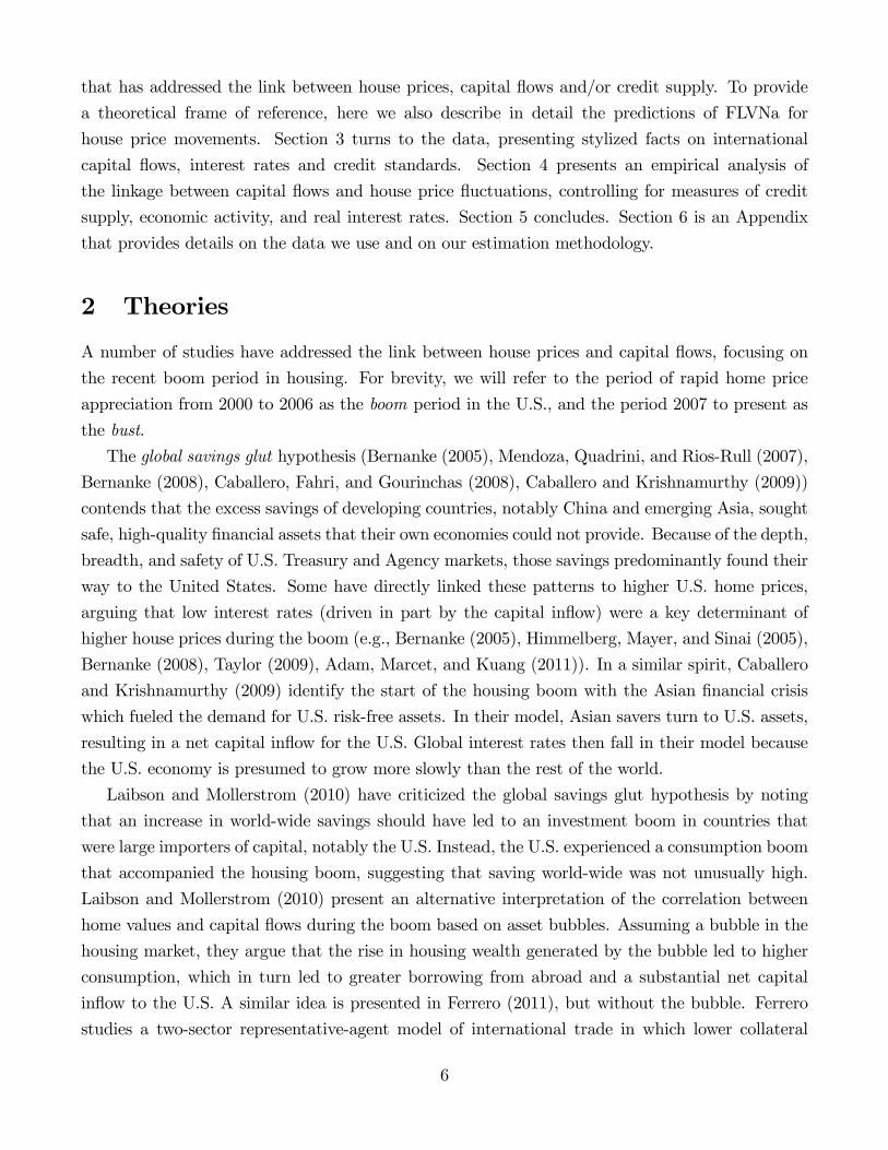
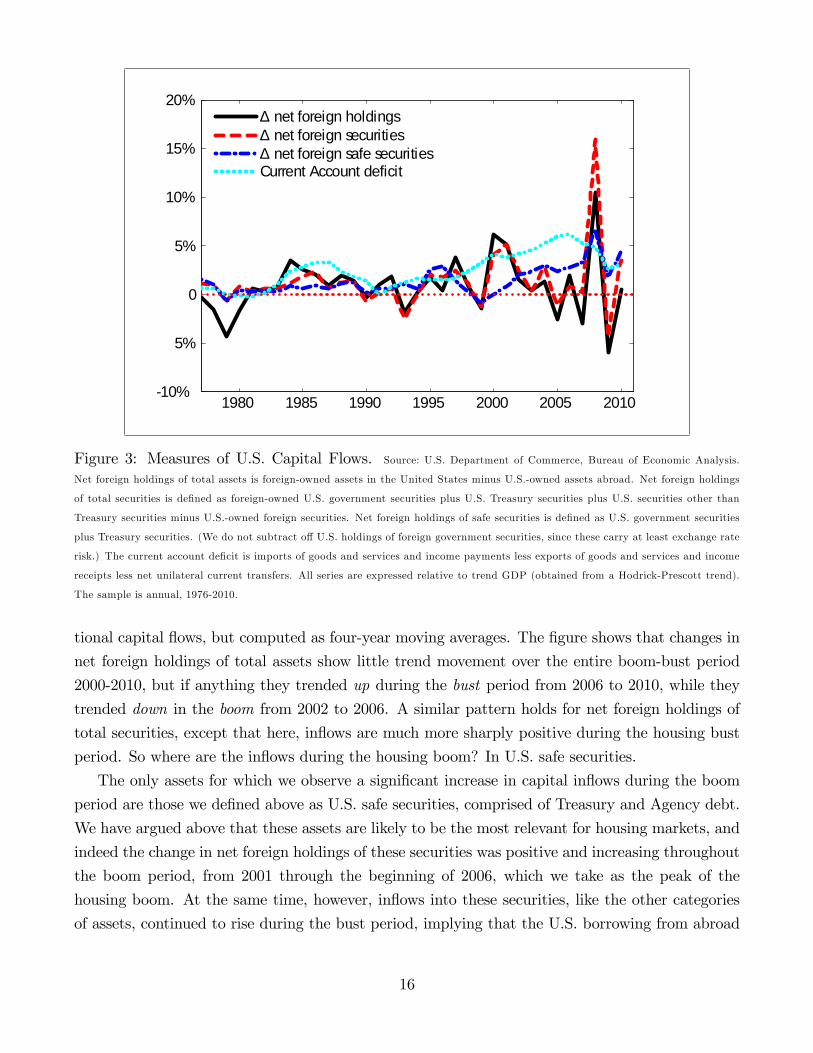
Figure 3 shows the movement in various measures of international capital flows into the United

States, relative to trend GDP, in annual data from 1976 to 2010. Plotted are the change in net

foreign holdings of total assets, total securities, and in what we will call U.S. “safe” securities

(defined as Treasuries and Agencies). We refer to a capital inflow as a positive change in holdings,

and vice versa for a capital outflow. Also plotted is the current account deficit. Figure 3 shows

that there is considerable volatility in these measures during housing boom and the subsequent

financial crisis, with particularly sharp increases in the change in net foreign holdings of U.S. assets

from 2007 to 2008. This corresponds to an upward spike in the change in the U.S. net foreign

liability position in 2008 (change in net foreign holdings of total assets in the figure). This series

declines from 2008 to 2009 and increases again from 2009 to 2010. Comparing the end-points of

these series in 2010 to their values in 2006, we see that—by any measure of assets—inflows (or the

change in holdings) were higher at the end of the sample in 2010 than they were at the peak of the

housing boom at the beginning of 2006 (end of 2005).

To get a better sense of the trends in these series, Figure 4 plots the same measures of interna-

15

1980 1985 1990 1995 2000 2005 2010­10%

5%

0

5%

10%

15%

20%∆ net foreign holdings∆ net foreign securities∆ net foreign safe securitiesCurrent Account deficit

Figure 3: Measures of U.S. Capital Flows. Source: U.S. Department of Commerce, Bureau of Economic Analysis.

Net foreign holdings of total assets is foreign-owned assets in the United States minus U.S.-owned assets abroad. Net foreign holdings

of total securities is defined as foreign-owned U.S. government securities plus U.S. Treasury securities plus U.S. securities other than

Treasury securities minus U.S.-owned foreign securities. Net foreign holdings of safe securities is defined as U.S. government securities

plus Treasury securities. (We do not subtract off U.S. holdings of foreign government securities, since these carry at least exchange rate

risk.) The current account deficit is imports of goods and services and income payments less exports of goods and services and income

receipts less net unilateral current transfers. All series are expressed relative to trend GDP (obtained from a Hodrick-Prescott trend).

The sample is annual, 1976-2010.

tional capital flows, but computed as four-year moving averages. The figure shows that changes in

net foreign holdings of total assets show little trend movement over the entire boom-bust period

2000-2010, but if anything they trended up during the bust period from 2006 to 2010, while they

trended down in the boom from 2002 to 2006. A similar pattern holds for net foreign holdings of

total securities, except that here, inflows are much more sharply positive during the housing bust

period. So where are the inflows during the housing boom? In U.S. safe securities.

The only assets for which we observe a significant increase in capital inflows during the boom

period are those we defined above as U.S. safe securities, comprised of Treasury and Agency debt.

We have argued above that these assets are likely to be the most relevant for housing markets, and

indeed the change in net foreign holdings of these securities was positive and increasing throughout

the boom period, from 2001 through the beginning of 2006, which we take as the peak of the

housing boom. At the same time, however, inflows into these securities, like the other categories

of assets, continued to rise during the bust period, implying that the U.S. borrowing from abroad

16

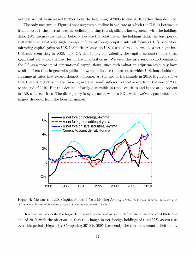
in these securities increased further from the beginning of 2006 to end 2010, rather than declined.

The only measure in Figure 4 that suggests a decline in the rate at which the U.S. is borrowing

from abroad is the current account deficit, pointing to a significant incongruence with the holdings

data. (We discuss this further below.) Despite the volatility in the holdings data, the bust period

still exhibited relatively high average inflows of foreign capital into all forms of U.S. securities,

mirroring capital gains on U.S. Liabilities relative to U.S. assets abroad, as well as a net flight into

U.S. safe securities, in 2008. The CA deficit (or, equivalently, the capital account) omits these

significant valuation changes during the financial crisis. We view this as a serious shortcoming of

the CA as a measure of international capital flows, since such valuation adjustments surely have

wealth effects that in general equilibrium would influence the extent to which U.S. households can

consume at rates that exceed domestic income. At the end of the sample in 2010, Figure 4 shows

that there is a decline in the (moving average trend) inflows to total assets from the end of 2008

to the end of 2010. But this decline is barely discernible in total securities and is not at all present

in U.S. safe securities. The discrepancy is again net flows into FDI, which we’ve argued above are

largely divorced from the housing market.

1980 1985 1990 1995 2000 2005 2010

­2%

0

2%

4%

6%∆ net foreign holdings, 4­yr ma∆ net foreign securities, 4­yr ma∆ net foreign safe securities, 4­yr maCurrent Account deficit, 4­yr ma

Figure 4: Measures of U.S. Capital Flows, 4-Year Moving Average. Notes: see Figure 3. Source: U.S. Departmentof Commerce, Bureau of Economic Analysis. The sample is annual, 1980-2010.

How can we reconcile the large decline in the current account deficit from the end of 2005 to the

end of 2010, with the observation that the change in net foreign holdings of total U.S. assets rose

over this period (Figure 3)? Comparing 2010 to 2005 (year end), the current account deficit fell by

17

$274,876 million, while the year-end change in net foreign holdings of total U.S. assets (relative to

trend GDP) rose by $395,440 million. The discrepancy is attributable to valuation effects, which

the current account ignores. Indeed, 126% of the discrepancy over this period is attributable to

valuation effects (-26% is attributable to a statistical discrepancy and other small adjustments

between the current and capital account flows). Thus, the decline in the current account deficit

from 2005 to 2010 suggests a decline in the rate at which U.S. liabilities are increasing, when

in fact this rate has increased, primarily because the change in capital gains foreign residents

enjoyed on U.S. assets from 2005 to 2010 far exceeded the change in capital gains accruing to

U.S. residents on their assets abroad. But these valuation adjustments came primarily from assets

other than what we have defined as U.S. safe assets. (This is perhaps not surprising since these

assets are far less volatile than is risky capital.) A break-down suggests that only 15.6% of these

valuation adjustments (specifically of the change in these adjustments from 2005 to 2010) came

from adjustments on U.S. safe assets. A much larger 39.7% came from financial securities other

than safe securities, and the majority (44.7%) came from valuation adjustments on assets other

than financial securities (including both safe and non-safe financial securities).

We can also compute the fraction of the cumulative change in net foreign holdings of safe assets

from the end of 2005 to the end of 2010 that is attributable valuation changes versus transactions.

Over this period, transactions account for 92.6%, while valuation changes account for just 7.3%.

This shows that, even accumulating over the entire bust period, there continues to be a strong

inflow of capital into U.S. safe securities that is not attributable merely to valuation changes.

To summarize, during the housing boom, only U.S. capital inflows on securities (equities,

corporate, U.S. Agency and Treasury bills and bonds) show any discernible upward trend. Among

securities, the upward trend has been driven almost entirely by an increase in net foreign holdings

of U.S. safe assets, specifically U.S. Treasury and Agency debt. Yet net inflows on these securities,

rather than declining during the housing bust, have continued to increase.

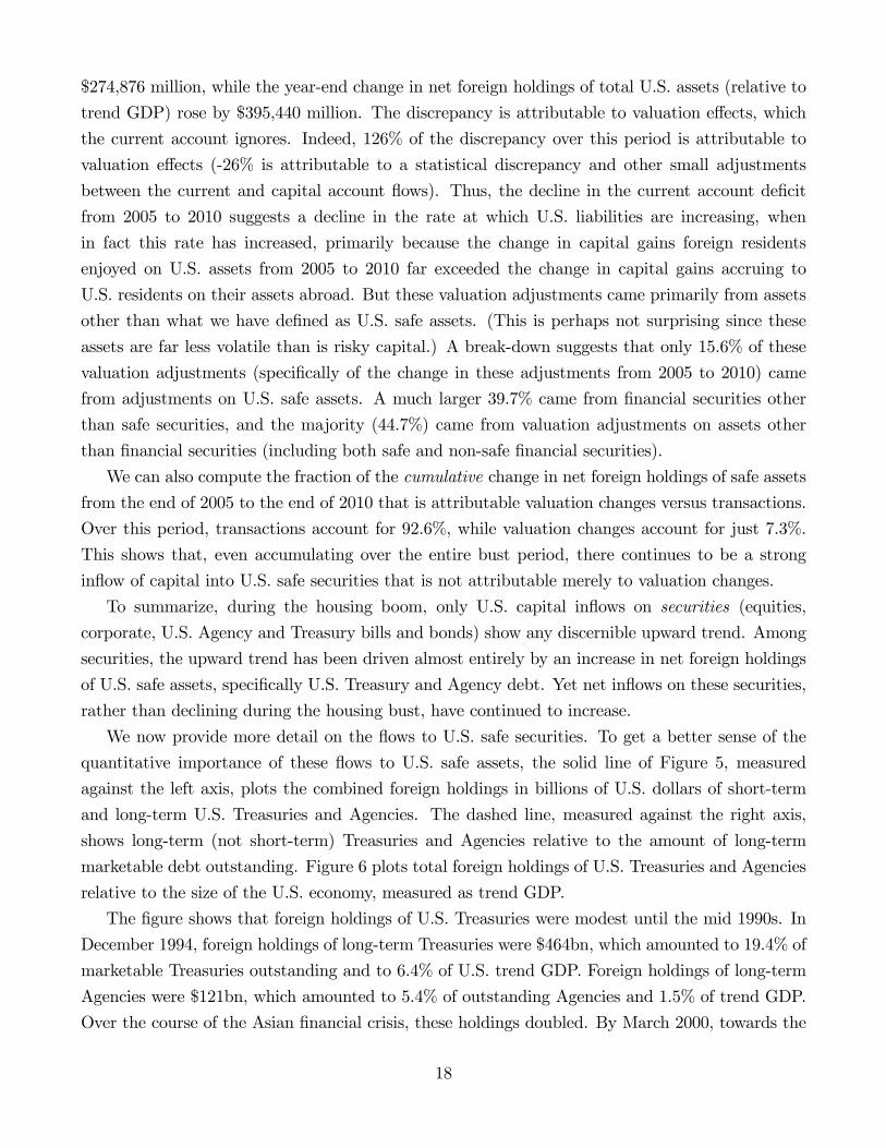
We now provide more detail on the flows to U.S. safe securities. To get a better sense of the

quantitative importance of these flows to U.S. safe assets, the solid line of Figure 5, measured

against the left axis, plots the combined foreign holdings in billions of U.S. dollars of short-term

and long-term U.S. Treasuries and Agencies. The dashed line, measured against the right axis,

shows long-term (not short-term) Treasuries and Agencies relative to the amount of long-term

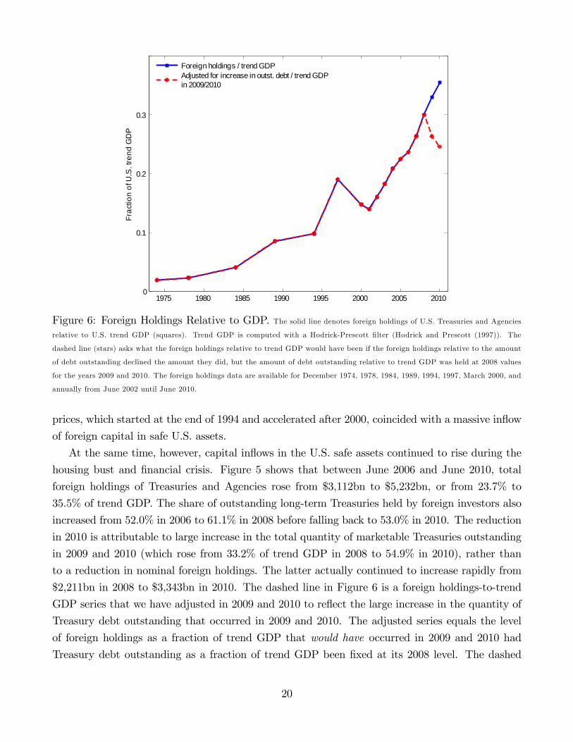
marketable debt outstanding. Figure 6 plots total foreign holdings of U.S. Treasuries and Agencies

relative to the size of the U.S. economy, measured as trend GDP.

The figure shows that foreign holdings of U.S. Treasuries were modest until the mid 1990s. In

December 1994, foreign holdings of long-term Treasuries were $464bn, which amounted to 19.4% of

marketable Treasuries outstanding and to 6.4% of U.S. trend GDP. Foreign holdings of long-term

Agencies were $121bn, which amounted to 5.4% of outstanding Agencies and 1.5% of trend GDP.

Over the course of the Asian financial crisis, these holdings doubled. By March 2000, towards the

18

1975 1980 1985 1990 1995 2000 2005 20100

1000

2000

3000

4000

5000

Fore

ign 

Hol

ding

s in

 Bill

ions

1975 1980 1985 1990 1995 2000 2005 20100

0.2

0.4

0.6

Fore

ign 

Hol

ding

s as

 Fra

ctio

n of

 Out

stan

ding

 Deb

t

TreasuriesAgencies

Figure 5: Foreign Holdings of U.S. Safe Assets. The figure plots foreign holdings of U.S. Treasuries (squares) and

U.S. Agencies (circles). U.S. Agencies denotes both the corporate bonds issued by the Government Sponsored Enterprizes and the

mortgage-backed securities guaranteed by them. The solid lines denote the amount of long-term and short-term holdings, in billions

of U.S. dollars, as measured against the left axis. The dashed lines denote the long-term foreign holdings relative to the total amount

of outstanding long-term (marketable) debt. Source: U.S. Treasury International Capital System’s annual survey of foreign portfolio

holdings of U.S. securities. The foreign holdings data are available for December 1974, 1978, 1984, 1989, 1994, 1997, March 2000, and

annually from June 2002 until June 2010.

end of the crisis, foreign holdings of long-term Treasuries and Agencies were $884bn and $261bn,

respectively, corresponding to 35.3% and 7.3% of the amounts outstanding. Total foreign holdings

of Treasuries and Agencies increased from 9.8% to 14.8% of trend GDP. Caballero, Fahri, and

Gourinchas (2008) argue that the Asian financial crisis represented a negative shock to the supply

of (investable/pledgeable) assets in East Asia, and led their investors to increase their investments

in U.S. bonds, one of the scarce risk-free assets available worldwide.

During housing boom from 2000-2006, the increase in foreign holdings of safe assets continued

at an even more rapid pace. Total foreign holdings of Treasuries and Agencies more than doubled

from $1,418bn in March 2000 to $3,112 in June 2006. Foreign holdings of long-term Treasuries went

from 35.3% to 52.0% of the total amount of Treasuries outstanding, while holdings of long-term

Agencies went from 7.3% to 17.2%. Most of the rise in foreign holdings of Treasuries took place

by 2004, while most of the rise in Agencies took place from 2004 to 2006. Total foreign holdings

of Treasuries and Agencies increased from 14.8% to 23.7% of trend GDP. The boom in U.S. house

19

1975 1980 1985 1990 1995 2000 2005 20100

0.1

0.2

0.3

Frac

tion 

of U

.S. t

rend

 GD

P

 Foreign holdings / trend GDP Adjusted for increase in outst. debt / trend GDP in 2009/2010

Figure 6: Foreign Holdings Relative to GDP. The solid line denotes foreign holdings of U.S. Treasuries and Agenciesrelative to U.S. trend GDP (squares). Trend GDP is computed with a Hodrick-Prescott filter (Hodrick and Prescott (1997)). The

dashed line (stars) asks what the foreign holdings relative to trend GDP would have been if the foreign holdings relative to the amount

of debt outstanding declined the amount they did, but the amount of debt outstanding relative to trend GDP was held at 2008 values

for the years 2009 and 2010. The foreign holdings data are available for December 1974, 1978, 1984, 1989, 1994, 1997, March 2000, and

annually from June 2002 until June 2010.

prices, which started at the end of 1994 and accelerated after 2000, coincided with a massive inflow

of foreign capital in safe U.S. assets.

At the same time, however, capital inflows in the U.S. safe assets continued to rise during the

housing bust and financial crisis. Figure 5 shows that between June 2006 and June 2010, total

foreign holdings of Treasuries and Agencies rose from $3,112bn to $5,232bn, or from 23.7% to

35.5% of trend GDP. The share of outstanding long-term Treasuries held by foreign investors also

increased from 52.0% in 2006 to 61.1% in 2008 before falling back to 53.0% in 2010. The reduction

in 2010 is attributable to large increase in the total quantity of marketable Treasuries outstanding

in 2009 and 2010 (which rose from 33.2% of trend GDP in 2008 to 54.9% in 2010), rather than

to a reduction in nominal foreign holdings. The latter actually continued to increase rapidly from

$2,211bn in 2008 to $3,343bn in 2010. The dashed line in Figure 6 is a foreign holdings-to-trend

GDP series that we have adjusted in 2009 and 2010 to reflect the large increase in the quantity of

Treasury debt outstanding that occurred in 2009 and 2010. The adjusted series equals the level

of foreign holdings as a fraction of trend GDP that would have occurred in 2009 and 2010 had

Treasury debt outstanding as a fraction of trend GDP been fixed at its 2008 level. The dashed

20

line shows that the increase in foreign holdings of U.S. Treasuries in 2009 and 2010 is less than

proportional to the increase in outstanding Treasuries over those years. In this relative sense,

therefore, foreigners have become less willing to hold U.S. Treasuries. According to the adjusted

series there is a reduction in foreign holdings as a fraction of trend GDP, from 30.0% of trend

GDP in 2008, to 24.6% in 2010, suggesting that a substantial “unwind”of foreign positions in U.S.

Treasuries may be underway, at least relative to the total amount of U.S. debt being issued.

Although there has so far been no reduction in nominal foreign holdings of U.S. Treasuries

during the housing bust, the financial crisis did lead to a substantial reduction in nominal foreign

holdings of U.S. Agencies. While foreign holdings of Agencies still rose from 17.2% in 2006 to 20.8%

of the amount outstanding in 2008, they fell back sharply to 15.6% of the amount outstanding in

2010 even as the amount outstanding remained flat.

Foreign Offi cial Holdings An important aspect of recent patterns in international capital flows

is that foreign demand for U.S. Treasury securities is dominated by Foreign Offi cial Institutions.

Krishnamurthy and Vissing-Jorgensen (2010) find that demand for U.S. Treasury securities by

governmental holders is extremely inelastic, implying that when these holders receive funds to

invest they buy U.S. Treasuries, regardless of their price. As explained in Kohn (2002), government

entities have specific regulatory and reserve currency motives for holding U.S. Treasuries and face

both legal and political restrictions on the type of assets that can be held, forcing them into safe

securities.

Data from the TIC system breaks out what share of foreign holdings of U.S. Treasuries is

attributable to Foreign Offi cial Institutions, which are government entities, mostly central banks.

Foreign Offi cial Institutions own the vast majority of U.S. Treasuries in recent data: in June 2010

Foreign Offi cial Institutions held 75% of all foreign holdings of U.S. Treasuries. That share has

always been high and has risen from 58% in March 2000 to 75% in June 2010. Indeed, 75%

represents a lower bound on the fraction of such securities held by Foreign Offi cial Institutions,

since some prominent foreign governments purchase U.S. securities through offshore centers and

third-country intermediaries, purchases that would not be attributed to Foreign Offi cial entities by

the TIC system—see Warnock and Warnock (2009). Foreign Offi cial Institutions also accounted for

64% of the foreign holdings of Agencies in June 2010.

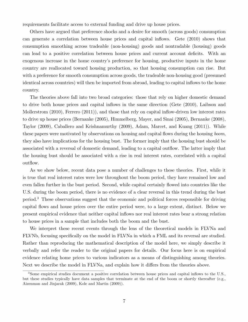
Asian central banks (China, Japan, Korea) have acquired massive U.S. dollar reserves in the

process of stabilizing their exchange rate. The share of foreign holdings is higher for long-term than

for short-term securities. The left panel of Figure 7 shows the foreign holdings as of December

2010 by country groups. China excludes Hong Kong, which is part of Rest of Asia. Banking

centers consist of the United Kingdom, the Caribbean, Luxembourg, Belgium, and Ireland. It is

widely believed that China holds a non-trivial fraction of its safe dollar assets through financial

intermediaries in the U.K. and in other banking centers Warnock (2010). The graph then suggests

21

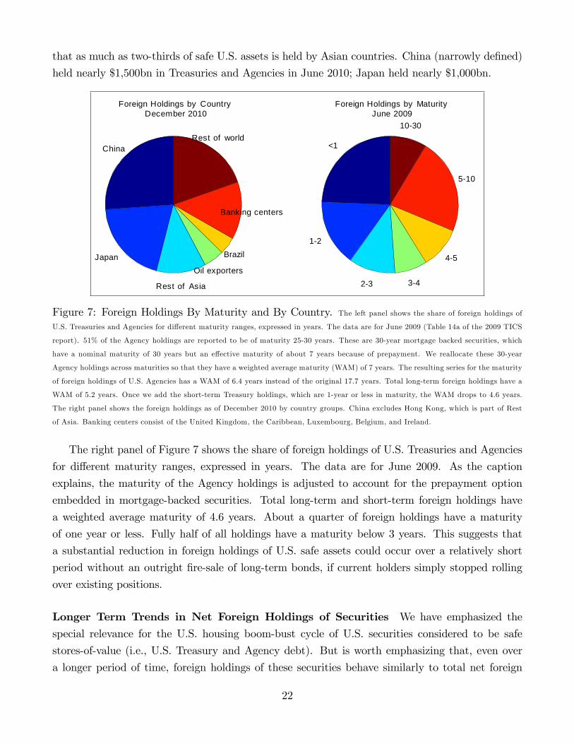
that as much as two-thirds of safe U.S. assets is held by Asian countries. China (narrowly defined)

held nearly $1,500bn in Treasuries and Agencies in June 2010; Japan held nearly $1,000bn.

China

 Japan

 Rest of  Asia

 Oil exporters

 Brazil

 Banking centers

 Rest of  world

Foreign Holdings by  Country December 2010

<1

1­2

2­3 3­4

4­5

5­10

10­30

Foreign Holdings by  Maturity June 2009

Figure 7: Foreign Holdings By Maturity and By Country. The left panel shows the share of foreign holdings ofU.S. Treasuries and Agencies for different maturity ranges, expressed in years. The data are for June 2009 (Table 14a of the 2009 TICS

report). 51% of the Agency holdings are reported to be of maturity 25-30 years. These are 30-year mortgage backed securities, which

have a nominal maturity of 30 years but an effective maturity of about 7 years because of prepayment. We reallocate these 30-year

Agency holdings across maturities so that they have a weighted average maturity (WAM) of 7 years. The resulting series for the maturity

of foreign holdings of U.S. Agencies has a WAM of 6.4 years instead of the original 17.7 years. Total long-term foreign holdings have a

WAM of 5.2 years. Once we add the short-term Treasury holdings, which are 1-year or less in maturity, the WAM drops to 4.6 years.

The right panel shows the foreign holdings as of December 2010 by country groups. China excludes Hong Kong, which is part of Rest

of Asia. Banking centers consist of the United Kingdom, the Caribbean, Luxembourg, Belgium, and Ireland.

The right panel of Figure 7 shows the share of foreign holdings of U.S. Treasuries and Agencies

for different maturity ranges, expressed in years. The data are for June 2009. As the caption

explains, the maturity of the Agency holdings is adjusted to account for the prepayment option

embedded in mortgage-backed securities. Total long-term and short-term foreign holdings have

a weighted average maturity of 4.6 years. About a quarter of foreign holdings have a maturity

of one year or less. Fully half of all holdings have a maturity below 3 years. This suggests that

a substantial reduction in foreign holdings of U.S. safe assets could occur over a relatively short

period without an outright fire-sale of long-term bonds, if current holders simply stopped rolling

over existing positions.

Longer Term Trends in Net Foreign Holdings of Securities We have emphasized the

special relevance for the U.S. housing boom-bust cycle of U.S. securities considered to be safe

stores-of-value (i.e., U.S. Treasury and Agency debt). But is worth emphasizing that, even over

a longer period of time, foreign holdings of these securities behave similarly to total net foreign

22

holdings of all securities. The reason is that foreign holdings of U.S. securities other than Treasuries

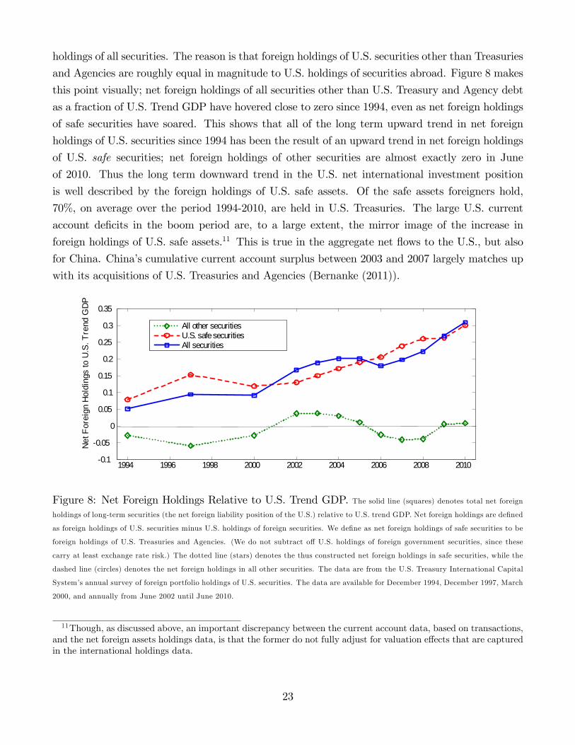
and Agencies are roughly equal in magnitude to U.S. holdings of securities abroad. Figure 8 makes

this point visually; net foreign holdings of all securities other than U.S. Treasury and Agency debt

as a fraction of U.S. Trend GDP have hovered close to zero since 1994, even as net foreign holdings

of safe securities have soared. This shows that all of the long term upward trend in net foreign

holdings of U.S. securities since 1994 has been the result of an upward trend in net foreign holdings

of U.S. safe securities; net foreign holdings of other securities are almost exactly zero in June

of 2010. Thus the long term downward trend in the U.S. net international investment position

is well described by the foreign holdings of U.S. safe assets. Of the safe assets foreigners hold,

70%, on average over the period 1994-2010, are held in U.S. Treasuries. The large U.S. current

account deficits in the boom period are, to a large extent, the mirror image of the increase in

foreign holdings of U.S. safe assets.11 This is true in the aggregate net flows to the U.S., but also

for China. China’s cumulative current account surplus between 2003 and 2007 largely matches up

with its acquisitions of U.S. Treasuries and Agencies (Bernanke (2011)).

1994 1996 1998 2000 2002 2004 2006 2008 2010­0.1

­0.05

0

0.05

0.1

0.15

0.2

0.25

0.3

0.35

Net

 For

eign

 Hol

ding

s to

 U.S

. Tre

nd G

DP

All other securitiesU.S. safe securitiesAll securities

Figure 8: Net Foreign Holdings Relative to U.S. Trend GDP. The solid line (squares) denotes total net foreignholdings of long-term securities (the net foreign liability position of the U.S.) relative to U.S. trend GDP. Net foreign holdings are defined

as foreign holdings of U.S. securities minus U.S. holdings of foreign securities. We define as net foreign holdings of safe securities to be

foreign holdings of U.S. Treasuries and Agencies. (We do not subtract off U.S. holdings of foreign government securities, since these

carry at least exchange rate risk.) The dotted line (stars) denotes the thus constructed net foreign holdings in safe securities, while the

dashed line (circles) denotes the net foreign holdings in all other securities. The data are from the U.S. Treasury International Capital

System’s annual survey of foreign portfolio holdings of U.S. securities. The data are available for December 1994, December 1997, March

2000, and annually from June 2002 until June 2010.

11Though, as discussed above, an important discrepancy between the current account data, based on transactions,and the net foreign assets holdings data, is that the former do not fully adjust for valuation effects that are capturedin the international holdings data.

23

Risky Mortgage Holdings Although net flows into securities other than Treasuries and Agen-

cies have hovered around zero, there were substantial gross flows across borders into private-label

products such as mortgage-backed securities (MBS), collateralized debt obligations (CDO), and

credit default swaps (CDS) with non-prime residential or commercial real estate as the underlying

or as the reference entity. Because an average of 80% of such private-label MBS principal received

a AAA rating from the credit ratings agencies and earned yields above those of Treasuries (see

U.S. Treasury Department (2011)), large foreign (as well as domestic) institutional investors were

able and willing to hold these assets on their books. The TICS data indicate that foreigners held

$594bn of non-agency mortgage-backed securities in June 2007. By June 2009, these holdings more

than halved to $266bn, after which they stabilized at $257bn in June 2010. Less than 10% of these

are held by foreign offi cial institutions (U.S. Treasury Department (2011)).

Bernanke (2011) shows interesting cross-country differences in the composition of countries’

U.S. investment portfolio. China and emerging Asia held three-quarters of their U.S. investments

in the form of Treasuries and Agencies in 2007. Their share of all AAA-rated securities was 77.5%,

while the AAA-rated share of all U.S. securities outstanding was only 36%. European (as well

as domestic) investors held only about one-third of their U.S. portfolio in the form of AAA-rated

assets. Not only did Europeans invest in non-AAA corporate debt, they accumulated $500bn in

U.S. asset-backed (largely mortgage-backed) securities between 2003 and 2007.

In addition to their different risk profiles over the housing cycle, Europe and Asia differ by

their current account positions. While the Asian economies ran a large current account surplus,

financing the purchases of U.S. assets with large trade surpluses, Europe had a balanced current

account over this period. It financed the purchases of risky U.S. assets by issuing external liabilities,

mostly equity, sovereign debt, and asset-backed commercial paper (ABCP). A prototypical example

of European holdings were AAA-rated tranches of subprime MBS held by large banks through

lightly-regulated off-balance sheet vehicles, and financed with ABCP (Acharya, Schnabl, and Suarez

(2010)).

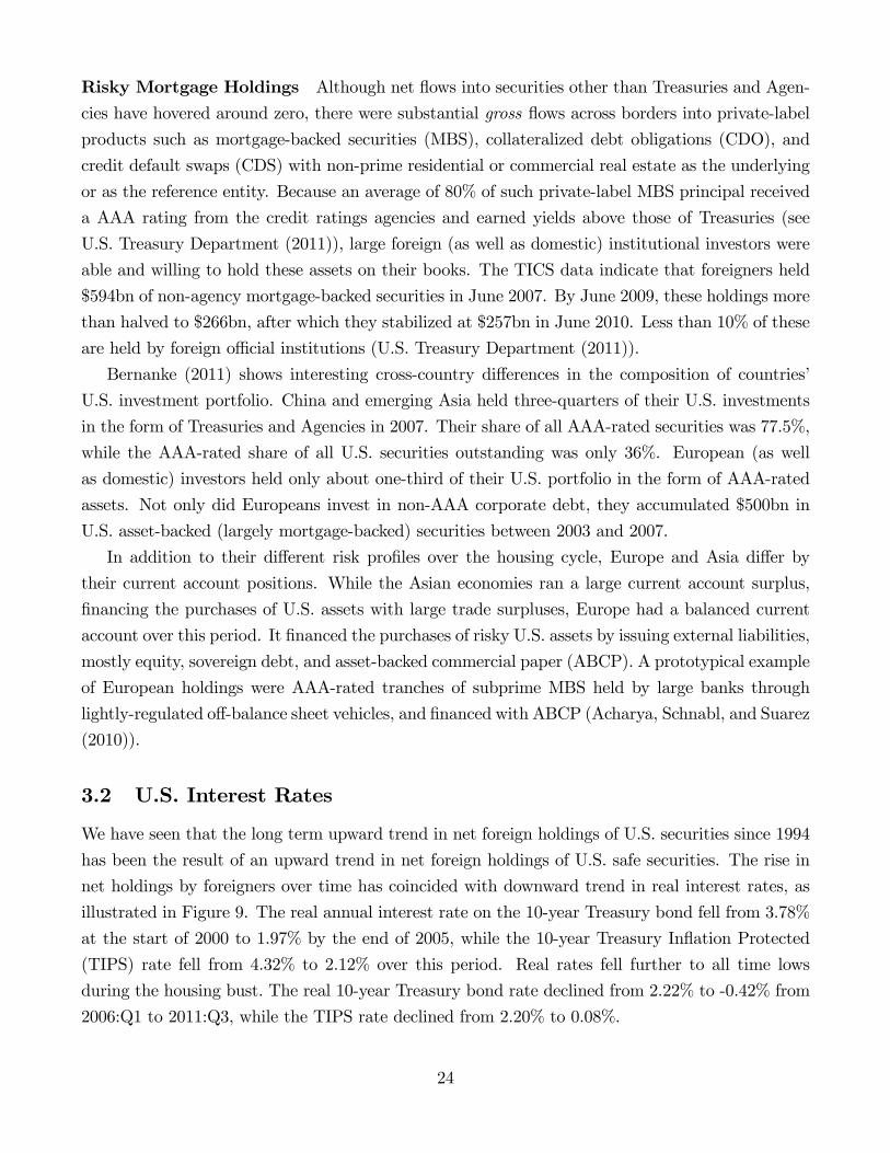
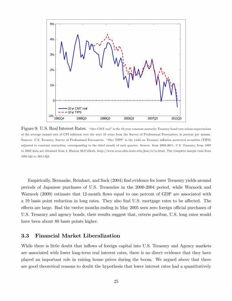
3.2 U.S. Interest Rates

We have seen that the long term upward trend in net foreign holdings of U.S. securities since 1994

has been the result of an upward trend in net foreign holdings of U.S. safe securities. The rise in

net holdings by foreigners over time has coincided with downward trend in real interest rates, as

illustrated in Figure 9. The real annual interest rate on the 10-year Treasury bond fell from 3.78%

at the start of 2000 to 1.97% by the end of 2005, while the 10-year Treasury Inflation Protected

(TIPS) rate fell from 4.32% to 2.12% over this period. Real rates fell further to all time lows

during the housing bust. The real 10-year Treasury bond rate declined from 2.22% to -0.42% from

2006:Q1 to 2011:Q3, while the TIPS rate declined from 2.20% to 0.08%.

24

1991Q4 1995Q3 1999Q3 2003Q3 2007Q3 2011Q3­1%

0

1%

2%

3%

4%

5%

10 yr CMT real10 yr TIPS

Figure 9: U.S. Real Interest Rates. “10yr CMT real”is the 10-year constant maturity Treasury bond rate minus expectationsof the average annual rate of CPI inflation over the next 10 years from the Survey of Professional Forecasters, in percent per annum.

Sources: U.S. Treasury, Survey of Professional Forecasters. “10yr TIPS” is the yield on Treasury inflation protected securities (TIPS)

adjusted to constant maturities, corresponding to the third month of each quarter. Source: from 2003-2011, U.S. Treasury, from 1997

to 2002 data are obtained from J. Huston McCulloch, http://www.econ.ohio-state.edu/jhm/ts/ts.html. The complete sample runs from

1991:Q4 to 2011:Q3.

Empirically, Bernanke, Reinhart, and Sack (2004) find evidence for lower Treasury yields around

periods of Japanese purchases of U.S. Treasuries in the 2000-2004 period, while Warnock and

Warnock (2009) estimate that 12-month flows equal to one percent of GDP are associated with

a 19 basis point reduction in long rates. They also find U.S. mortgage rates to be affected. The

effects are large. Had the twelve months ending in May 2005 seen zero foreign offi cial purchases of

U.S. Treasury and agency bonds, their results suggest that, ceteris paribus, U.S. long rates would

have been about 80 basis points higher.

3.3 Financial Market Liberalization

While there is little doubt that inflows of foreign capital into U.S. Treasury and Agency markets

are associated with lower long-term real interest rates, there is no direct evidence that they have

played an important role in raising house prices during the boom. We argued above that there

are good theoretical reasons to doubt the hypothesis that lower interest rates had a quantitatively

25

large effect on house prices during the boom. Empirically, Glaeser, Gottlieb, and Gyourko (2010)

concur and find that even when the house price impact of lower interest rates should be stronger

(at a low initial rate), they account for at most 1/5 of the observed change in housing prices. We

present additional evidence on this below.

What then accounts for the dramatic rise in U.S. house prices during the boom if not low

interest rates? A key missing element in this scenario is the shift in credit standards and housing

transactions costs, summarized above as a FML and its reversal. The widespread relaxation of

credit standards is well documented (see Nichols, Pennington-Cross, and Yezer (2005), Favilukis,

Ludvigson, and Van Nieuwerburgh (2009), Ferrero (2011) for more details). Moreover, a growing

body of empirical evidence directly links measures that identify changes in credit supply (as opposed

to changes in demand) to movements in asset prices.

3.3.1 Loan-to-Value Ratios

Many different aspects of mortgage lending over the 2000-2010 period are consistent with a re-

laxation of credit standards. It may seem that an obvious way to measure relaxation of credit

standards is to study loan-to-value ratios. Several studies have observed that average or median

loan-to-value ratios did not increase much over time; see for example the contribution by Glaeser,

Gottlieb, and Gyourko (2010) in this volume. There are at least three problems with using average

LTV ratios as an indicator of tightness of credit constraints. First, average loan-to-value ratio mea-

sures usually mix in mortgages for house purchases with those for refinancing. The latter category

of have much lower LTV ratios because the borrowers often have accumulated substantial amounts

of home equity already. These refinancing are quantitatively important because, during the hous-

ing boom, mortgage interest rates came down persistently, leading to a massive refinancing boom.

The share of refis in originations was 63% in 2002, 72% in 2003, and around 50% in 2004-2006

(Inside Mortgage Finance data).

Second, the average loan-to-value ratio are typically based only on the first lien on the house.

But often, new borrowers would take out an 80% LTV first lien and then a second (and possibly

third) lien (closed-end second or home equity line of credit). By the end of 2006 households routinely

were able to buy homes with 100% or higher financing using a piggyback second mortgage or home

equity loan. The fraction of households with second liens rose dramatically during the boom. For

subprime loans, that fraction rose from 3% in 2002 to 30%; for Alt-A loans it rose from 3% to

44%.12 In addition, second or third liens were the often the way in which existing home owners

tapped into their home equity, often several quarters after they took out the original mortgage.

12An indirect indicator of the prevalence of the use of second mortgages is that the fraction of first liens withLTV exactly equal to 80% rose substantially between 2002 and 2006 Krainer, LeRoy, and Munpyung (2009). Theyshow that the fraction of FRMs with exactly 80% LTV decreased from 22% to 6% over this period, the presumptionbeing that a rising share of these 80% LTV loans were associated with second liens.

26

This equity extraction through second liens is in addition to extraction via cash-out refinancing,

another innovation of the boom which became increasingly prevalent. The contribution in this

volume by Lee, Mayer, and Tracy (2011) shows that second lien balances grew from about $200

billion at the start of 2002 to over $1 trillion by the end of 2007. It also shows that the prevalence

of second mortgages rose in every U.S. region from below 10% at the start of the boom (bit higher

in coastal cyclical markets) to around 40% in 2006 (except for the Midwest declining region which

peaks at a 20% share).

What this evidence suggests is that we should look at combined LTVs (CLTVs), combining

all liens on a property, at the time of purchase. And to gauge how credit constraints affected

the marginal household, we should look at the right tail of that CLTV distribution. Lee, Mayer,

and Tracy (2011) show that the average LTV at purchase for properties with one lien stayed

rather constant over the boom, if anything it declined a bit. Likewise, the share of purchases with

one mortgage with an LTV greater or equal to 95% also stays constant. By contrast, the share of

purchases with multiple mortgages with a CLTV greater or equal to 95% rises dramatically in every

region. The nationwide increase is from about a 25% share to about a 60% share. At the peak,

about two-thirds of purchase mortgages with a second lien had a CLTV of 95% or more. Keys,

Piskorski, Seru, and Vig (2011), also in this volume, show that the average CLTV on subprime

loans increases from 80% in 1997 to 96% in 2006.

A recent study using detailed data on mortgages in Los Angeles county shows the dramatic

easing of credit constraints over the boom period and subsequent reversal in another way. Figure 10

from Laufer (2011) shows the share of properties in LA country with CLTVs at purchase above 100%

for all loans except non-conventional loans (FHA and VA loans). That share rises from 8% in 2001

to 54% in the fourth quarter of 2006, before collapsing. The sharp drop in this series beginning in

2007 and reaching zero by 2008 reflects a significant reduction in the maximum LTV ratio permitted

by mortgage originators, since home values (in the denominator) were simultaneously falling.

Third, there is a widespread belief that house price appraisals, done at the time of mortgage

origination, were upward biased during the boom. This would downward bias LTV and CLTV

ratios. As a result, what may look like flat or modestly increasing (average) CLTVs may in fact

be increasing CLTVs once measured relative to the true value of the property.

3.3.2 Other Aspects of Credit Availability

The behavior of CLTV ratios in the boom and bust does not do full justice to several aspects

of the increased availability of mortgage credit. New mortgage products became available to

borrowers that were previously unable to obtain mortgage credit. The share of subprime mortgage

originations (to borrowers with low FICO credit scores) went from less than 10% of originations

in 2002 to 40% of originations by 2006, growing from 120 billion in originations in 2001 to 600

27

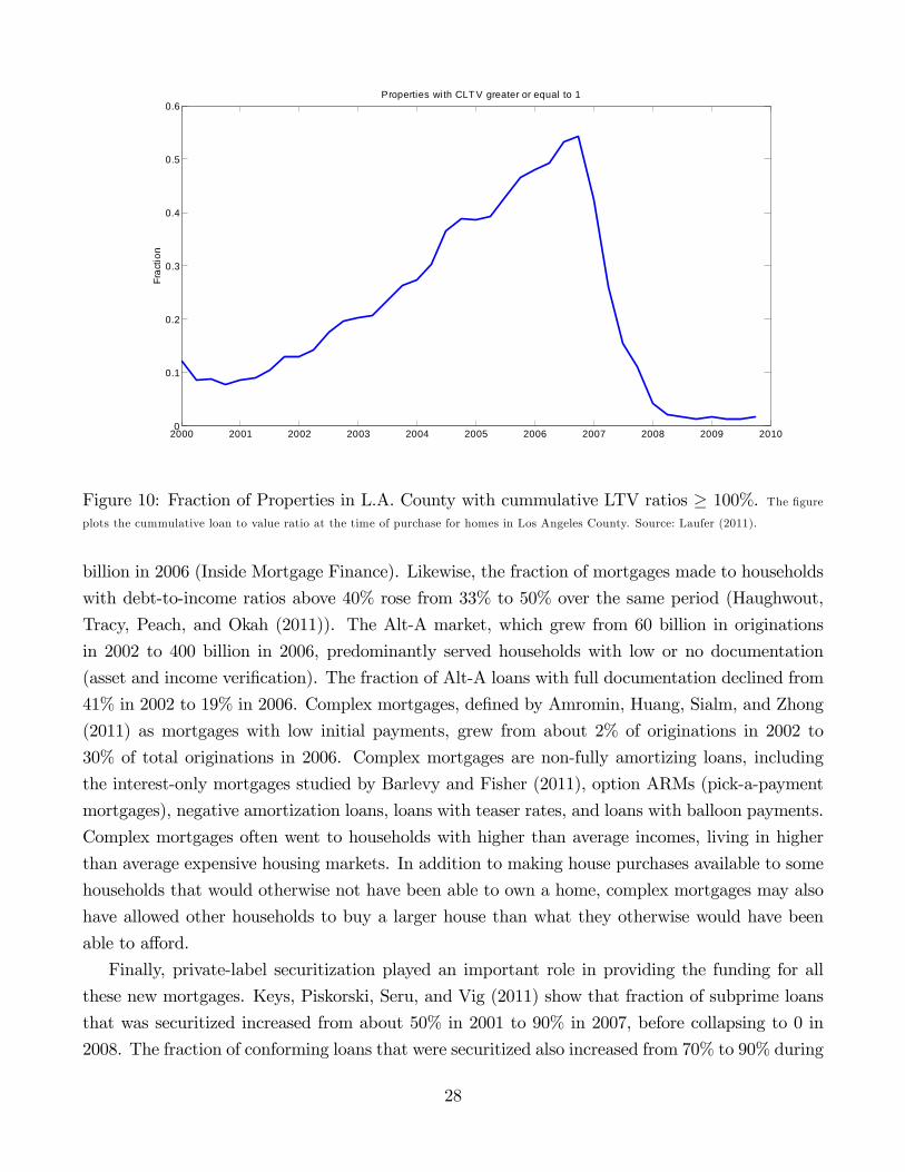
2000 2001 2002 2003 2004 2005 2006 2007 2008 2009 20100

0.1

0.2

0.3

0.4

0.5

0.6

Frac

tion

Properties with CLT V greater or equal to 1

Figure 10: Fraction of Properties in L.A. County with cummulative LTV ratios ≥ 100%. The figureplots the cummulative loan to value ratio at the time of purchase for homes in Los Angeles County. Source: Laufer (2011).

billion in 2006 (Inside Mortgage Finance). Likewise, the fraction of mortgages made to households

with debt-to-income ratios above 40% rose from 33% to 50% over the same period (Haughwout,

Tracy, Peach, and Okah (2011)). The Alt-A market, which grew from 60 billion in originations

in 2002 to 400 billion in 2006, predominantly served households with low or no documentation

(asset and income verification). The fraction of Alt-A loans with full documentation declined from

41% in 2002 to 19% in 2006. Complex mortgages, defined by Amromin, Huang, Sialm, and Zhong

(2011) as mortgages with low initial payments, grew from about 2% of originations in 2002 to

30% of total originations in 2006. Complex mortgages are non-fully amortizing loans, including

the interest-only mortgages studied by Barlevy and Fisher (2011), option ARMs (pick-a-payment

mortgages), negative amortization loans, loans with teaser rates, and loans with balloon payments.

Complex mortgages often went to households with higher than average incomes, living in higher

than average expensive housing markets. In addition to making house purchases available to some

households that would otherwise not have been able to own a home, complex mortgages may also

have allowed other households to buy a larger house than what they otherwise would have been

able to afford.

Finally, private-label securitization played an important role in providing the funding for all

these new mortgages. Keys, Piskorski, Seru, and Vig (2011) show that fraction of subprime loans

that was securitized increased from about 50% in 2001 to 90% in 2007, before collapsing to 0 in

2008. The fraction of conforming loans that were securitized also increased from 70% to 90% during

28

the boom, and has stabilized at that level.

3.3.3 Exogenous Changes in Credit Supply

Moreover, a growing body of empirical evidence directly links measures that identify changes in

credit supply (as opposed to changes in demand) to movements in asset prices.

Adelino, Schoar, and Severino (2011) exploit exogenous variation in the government-controlled

conforming loan limit (CLL) as an instrument for changing credit supply. The CLL determines

the maximum size of a mortgage that can be purchased or securitized by Fannie Mae or Freddie

Mac. Because these loans were widely understood to have the implicit (and since 2008 explicit)

backing of the U.S. government, borrowers in the market for loans that fall below the CLL have

easier access to credit at less costly terms. Changes in the CLL are set annually and depend on

the previous year’s limit plus the change in the median national house price. These movements

are clearly exogenous to individual mortgage transactions, local housing markets, and the local

economy. Using data on single-family house purchases in 10 metropolitan statistical areas between

1998 and 2006, Adelino et. al. show that houses that became newly eligible for a conforming loan

just after an increase in the CLL saw significant price increases relative to similar houses that were

already below the limit before the CLL increase.

Rajan and Ramcharan (2011a) exploit interstate banking restrictions to study the effect of

credit supply on land prices in the early 20th century U.S. Regulations at the time stipulated that

banks could not lend across state borders. They argue that the number of banks in this era proxied

for credit supply, with more banks indicating higher supply. They show that the number of banks

in a county positively predicts land prices independently of fundamentals likely to move credit

demand for land (commodity prices). They also find that the number of banks in neighboring

in-state counties affects land prices more than the number of banks in equidistant counties out-

of-state. Since banks were prohibited from lending across state borders, it is diffi cult to form a

coherent story for this latter fact that does not involve credit supply.

In a similar spirit, Favara and Imbs (2011) identify movements credit supply in more recent

data (since 1994) by studying bank branching restrictions. Even though interstate banking (i.e.,

cross-state ownership of banks) was made legal after the passage of the Interstate Banking and

Branching Effi ciency Act of 1994, U.S. states retained the right to erect barriers to interstate

branching. They study branching deregulations since 1994 and show that they significantly affect

the supply of mortgage credit. With deregulation, the number and volume of originated mortgage

loans rise, while denial rates fall, echoing evidence in Mian and Sufi (2009), discussed below. This

deregulation has no effect on a placebo sample, formed of independent mortgage companies that

should not be affected by the regulatory changes. Deregulation leads to greater supply of mortgage

credit, which they find leads to significantly higher house prices.

29

Our main measure of credit availability is based on quarterly bank lending surveys for countries

in the Euro area and the U.S. For the U.S., we use the Senior Loan Offi cer Opinion Survey on Bank

Lending Practices (SLOOS), collected by the Federal Reserve. An important aspect of this survey

is that it asks banks to explicitly distinguish between changes in the supply of credit as distinct

from the demand for credit, on bank loans to businesses and households over the past three months.

Thus in principal, answers to the appropriate questions are able to identify a movement in supply

separately from a movement in demand. We focus on questions related to mortgage credit supply to

households. The detailed information is considered highly reliable because the surveys are carried

out by central banks which are also bank regulators with access to a large amount of information

about a bank’s operations, including those reflected in loan applications and balance sheet data.

Data for other countries are from bank lending surveys conducted by national central banks,

and the European Central Bank. The survey questions are modeled after the U.S. Survey of Senior

Loan Offi cers. (See the Appendix for data sources.) We use these data below in our empirical

analysis.

For the U.S. SLOOS survey, banks indicate easing, tightening, or no change in lending standards

compared to the previous three months. We use the net percentage of banks that have eased their

lending standards on mortgage loans as a measure of credit supply. This is the difference between

the percentage of banks reporting easing and the percentage of banks reporting tightening, thus a

positive figure indicates a net easing of lending standards, considering all bank respondents.

Figure 11 reports the net percentage of banks easing over time. We denote this variable CSt.

According to this measure, there was a significant easing of standards from 2002-2006, and a very

sharp tightening afterwards. Notice that this measure does not weight banks by their relative

importance in the mortgage market, nor does it weight the responses by the degree of tightening.

Thus, it is not an indicator of the strength of credit easing or tightening, only of its breadth.

Moreover, until 2007, the survey did not distinguish between prime and subprime mortgages. The

figure shows clearly a broad tightening of credit standards beginning in the end of 2006. A cursory

investigation of the figure suggests that the easing of standards in the boom was more modest. One

must be careful in interpreting this series however. There is a long string of observations starting

in 1998 and continuing through 2006 that show a net easing of credit standards. Recall that the

survey asks bank’s about how their standards have changed relative to the pervious three months.

Thus a series of observations indicating easier credit conditions relative to previous quarters by a

few important banks in the mortgage space, once cumulated, could indicate a significant relaxation

of underwriting standards.

We can relate CS to the growth in mortgages outstanding. Before doing so, Figure 12 shows the

share of mortgages outstanding by holder, over time. The line labeled “GSE portfolio and pools”

are Agency and GSE-backed mortgage pools, comprised only by conforming mortgage loans.13 The

13Prior to 2010:Q1, only a small fraction of GSE-mortgage pools were held in portfolio at Fannie Mae and Freddie

30

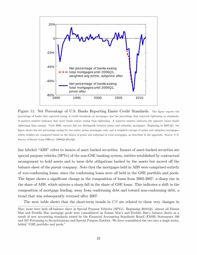
1990 1995 2000 2005 2010­80%

­60%

­40%

­20%

0

20%

 Net percentage of banks easing total mortgages unti l 2006Q1, weighted avg prime, subprime after

 Net percentage of banks easing total mortgages unti l 2006Q1, prime after

Figure 11: Net Percentage of U.S. Banks Reporting Easier Credit Standards. The figure reports the

percentage of banks that reported easing of credit standards on mortgages, less the percentage that reported tightening os standards.

A positive number indicates that more banks report easing than tightening. A negative number indicates the opposite (more banks

tightening than easing). Until 2006, surveys did not distinguish between prime and subprime mortgages. Beginning in 2007:Q1, the

figure shows the net percentage easing for two series: prime mortgages only, and a weighted average of prime and subprime mortgages,

where weights are computed based on the shares of prime and subprime in total mortgages, as described in the appendix. Source: U.S.

Survey of Senior Loan Offi cers, 1990Q2-2011Q2.

line labeled “ABS”refers to issuers of asset backed securities. Issuers of asset-backed securities are

special purpose vehicles (SPVs) of the non-GSE banking system, entities established by contractual

arrangement to hold assets and to issue debt obligations backed by the assets but moved off the

balance sheet of the parent company. Note that the mortgages held in ABS were comprised entirely

of non-conforming loans, since the conforming loans were all held in the GSE portfolio and pools.

The figure shows a significant change in the composition of loans from 2002-2007: a sharp rise in

the share of ABS, which mirrors a sharp fall in the share of GSE loans. This indicates a shift in the

composition of mortgage lending, away from conforming debt and toward non-conforming debt, a

trend that was subsequently reversed after 2007.

The next table shows that the short-term trends in CS are related to these very changes in

Mac; most were held off-balance sheet in Special Purpose Vehicles (SPVs). Beginning 2010:Q1, almost all FannieMae and Freddie Mac mortgage pools were consolidated on Fannie Mae’s and Freddie Mac’s balance sheets as aresult of new accounting standards issued by the Financial Accounting Standards Board (FASB) Statements 166and 167 Pertaining to Securitizations and Special Purpose Entities. We have consoldated the two into a single series,labled “GSE portfolio and pools.”

31

1990 1992 1994 1996 1998 2000 2002 2004 2006 2008 2010 20120

0.1

0.2

0.3

0.4

0.5

0.6

Sha

re o

f Tot

al H

ome 

Mor

tgag

es

U.S.­Chartered Commercial BanksSavings InstitutionsGSE portfolio and poolsABS

Figure 12: Mortgage Shares By Holder Over Time. “ABS”are home mortgages by Issuers of asset-backed securitieswhich are special purpose vehicles’(SPVs), entities established by contractual arrangement to hold assets and to issue debt obligations

backed by the assets. “U.S. Chartered Commercial Banks” refers to mortgages held by U.S.-chartered commercial banks. “Savings

Institutions” refers to state-chartered savings banks, federal savings banks, cooperative banks, and savings and loan associations. GSE

portfolio and pools refers to mortgages held as MBS assets in the portfolio of Government Sponsored Enterprises plus mortgages held

in Agency- and GSE backed-Mortgage pools not on GSE balance sheets prior to 2010:Q1. Data are from Federal Reserve, flow of funds,

table L.218. Sample 1990Q1-2011Q2.

the composition of lending over the boom/bust period. We investigate the relation between the

four-quarter moving average value of the SLOOS net percentage indicator CS shown in Figure 11,

and year-over-year growth in mortgage credit outstanding, by holder. The table reports results

from a regression of the latter on the former. The first column shows the relation over the full

sample 1991:Q1-2010:Q4. This column shows that CS is positively related to growth in ABS and

negatively related to growth in mortgages held in GSE pools. The last row shows the results from

a regression of the ratio of ABS to GSE pools. CS is positively related to growth in this ratio.

Thus the percentage of banks reporting an easing of credit standards is associated with a shift

in the composition of loans, toward non-conforming loans and away from conforming loans. The

subsequent columns show that this result is unique to the boom-bust period 2000-2010. In both

the boom (2000-2006) and bust (2007-2010), CS is positively related to the ratio ABS/GSE, but

it is negatively related to this ratio in the years prior to this boom/bust cycle (1991:Q1-1999:Q4).

32

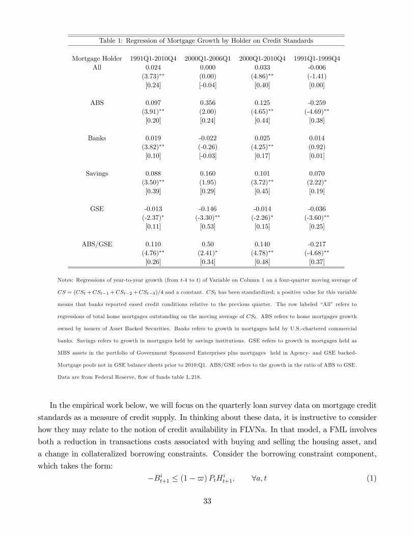
Table 1: Regression of Mortgage Growth by Holder on Credit Standards

Mortgage Holder 1991Q1-2010Q4 2000Q1-2006Q1 2000Q1-2010Q4 1991Q1-1999Q4All 0.024 0.000 0.033 -0.006

(3.73)∗∗ (0.00) (4.86)∗∗ (-1.41)[0.24] [-0.04] [0.40] [0.00]

ABS 0.097 0.356 0.125 -0.259(3.91)∗∗ (2.00) (4.65)∗∗ (-4.69)∗∗

[0.20] [0.24] [0.44] [0.38]

Banks 0.019 -0.022 0.025 0.014(3.82)∗∗ (-0.26) (4.25)∗∗ (0.92)[0.10] [-0.03] [0.17] [0.01]

Savings 0.088 0.160 0.101 0.070(3.50)∗∗ (1.95) (3.72)∗∗ (2.22)∗

[0.39] [0.29] [0.45] [0.19]

GSE -0.013 -0.146 -0.014 -0.036(-2.37)∗ (-3.30)∗∗ (-2.26)∗ (-3.60)∗∗

[0.11] [0.53] [0.15] [0.25]

ABS/GSE 0.110 0.50 0.140 -0.217(4.76)∗∗ (2.41)∗ (4.78)∗∗ (-4.68)∗∗

[0.26] [0.34] [0.48] [0.37]

Notes: Regressions of year-to-year growth (from t-4 to t) of Variable on Column 1 on a four-quarter moving average of

CS = (CSt +CSt−1 +CSt−2 +CSt−3)/4 and a constant. CSt has been standardized; a positive value for this variable

means that banks reported eased credit conditions relative to the previous quarter. The row labeled “All” refers to

regressions of total home mortgages outstanding on the moving average of CSt. ABS refers to home mortgages growth

owned by issuers of Asset Backed Securities. Banks refers to growth in mortgages held by U.S.-chartered commercial

banks. Savings refers to growth in mortgages held by savings institutions. GSE refers to growth in mortgages held as

MBS assets in the portfolio of Government Sponsored Enterprises plus mortgages held in Agency- and GSE backed-

Mortgage pools not in GSE balance sheets prior to 2010:Q1. ABS/GSE refers to the growth in the ratio of ABS to GSE.

Data are from Federal Reserve, flow of funds table L.218.

In the empirical work below, we will focus on the quarterly loan survey data on mortgage credit

standards as a measure of credit supply. In thinking about these data, it is instructive to consider

how they may relate to the notion of credit availability in FLVNa. In that model, a FML involves

both a reduction in transactions costs associated with buying and selling the housing asset, and

a change in collateralized borrowing constraints. Consider the borrowing constraint component,

which takes the form:

−Bit+1 ≤ (1−$)PtH

it+1, ∀a, t (1)

33

where Bit+1 is the amount of bonds household i owns at the beginning of period t + 1, Pt denotes

the relative price of housing in units of the non-housing consumption good (Pt is the time t price of

a unit of housing of fixed quality and quantity), and H it+1 is the housing stock owned by household

i and the beginning of period t + 1. A negative value for Bi indicates a borrowing position. This

equation represents the collateral constraint in the model, where 0 ≤ $ ≤ 1. It says that households

may borrow no more than a fraction (1−$) of the value of housing, implying that they must post

collateral equal to a fraction $ of the value of the house. This constraint can be thought of as a

down-payment constraint for new home purchases, but it also encompasses collateral requirements

for home equity borrowing against existing homes. The constraint gives the maximum combined

loan-to-value (LTV) ratio for first and second mortgages and home equity withdrawal.

FLVNa asks how a plausibly calibrated change in its value (along with a calibrated change in

housing transactions costs) changes the equilibrium outcome. Thus, one way credit supply can

change is via a change in the fraction (1−$) of the home’s value that must be held as collateral.

But, as discussed above, borrowing capacity will fluctuate endogenously with the collateral value

pHt Hit+1 even if that fraction remains unchanged. This represents an endogenous change in bor-

rowing capacity, driven by economic shocks and accompanied by revisions in expectations about

future economic conditions. These factors get immediately reflected in house prices, which affects

borrowing capacity and the tightness of constraints. We argue that either of these represent a

change in credit supply in the sense that they are related to a borrower’s access to funds via her

credit constraint. Moreover, the two could be correlated (expectations of a decline in economic

activity could lead to an increase in $), as they are in the transition dynamics studied by FLVNa

and displayed in Figure 2 above.14

4 International Evidence on House Price Fluctuations

We have seen above that the U.S. experienced large capital inflows and commensurate current

account deficits at the same time that it experienced strong growth in house prices. The same

is true for countries such as Iceland, Ireland, and Spain. In fact, during the boom, there is a

positive cross-country correlation of current account deficits with house price growth on the one

hand (Ferrero (2011), Laibson and Mollerstrom (2010), Gete (2010)) and with value added and

the labor share of the construction industry on the other hand (Gete (2010)). Using data that

ends before the bust, Aizenman and Jinjarak (2009) provide a precise estimate of the relationship

between house prices and external imbalances: a one standard deviation increase in lagged current

14The transition dynamics are an exploration of movements between stochastic states with different values for $(as well as the housing transactions costs). An important aspect of the transition is that the exogenous changesin borrowing capacity are correlated with endogenous changes in borrowing capacity, because the exogenous andunexpected decline in $ is calibrated to coincide with an economic boom, which bolsters collateral values andendogenously relaxes borrowing constraints.

34

account deficits is associated with a 10% appreciation of real estate prices.

Panel A of Table 2 replicates the flavor of these results for the boom period and extends the

sample to a larger set of countries. It reports real house price growth (deflated by CPI), cumulative

current account deficits, and cumulative residential investment over the period 2000:Q1 to 2006:Q4,

with the last two variables measured relative to GDP in 2006:Q4. Countries such as Germany,

Switzerland, China, and Austria accumulated large current account surpluses and exhibited slow

house price growth and modest residential investment, while countries such as the U.S., Spain, the

U.K., Portugal, Greece, Estonia, New Zealand, and Australia attracted lots of external capital,

exhibited large rises in house prices, and experienced significant residential investment booms. In

the boom period, there is a positive cross-country correlation between average house price changes

and average current account deficits equal to 23%. There is also a negative cross-country correlation

between residential investment an house price growth: countries with more residential investment

experienced lower house price growth, consistent with the idea that residential investment drives

up the expected housing stock and drives down the expected future growth rate on the dividend

to housing (rent).

It is tempting to conclude that the excess savings of the first group of countries found its way

to the real estate industry in the second group of countries and fueled the housing boom there.

However, as argued above, general equilibrium considerations suggest that large inflows into safe

assets need not lead to large house price booms because the effect of lower interest rates is offset by a

rise in risk premia and an expected increase in the housing stock from higher residential investment.

This may help explain why the current account patterns from the boom period persisted in many

countries during the housing bust, while house prices and residential investment patterns obviously

did not. Panel B of Table 2 shows that the cross-country correlation between house price changes

and current account dynamics reverses in the bust sample from 2006:Q4 to 2010:Q4. The cross-

country correlation between the current account deficit and house price growth is now −38%. By

itself, this negative correlation is certainly not consistent with the notion that capital inflows cause

higher house price growth. Nor is it consistent with the hypothesis that capital inflows lead to a

relaxation of credit standards, which in turn causes higher house price growth. To further explore

these issues, we now turn to a statistical analysis of the relation between house price changes (or

changes in price-rent ratios), measures of capital flows, credit standards and interest rates.

35

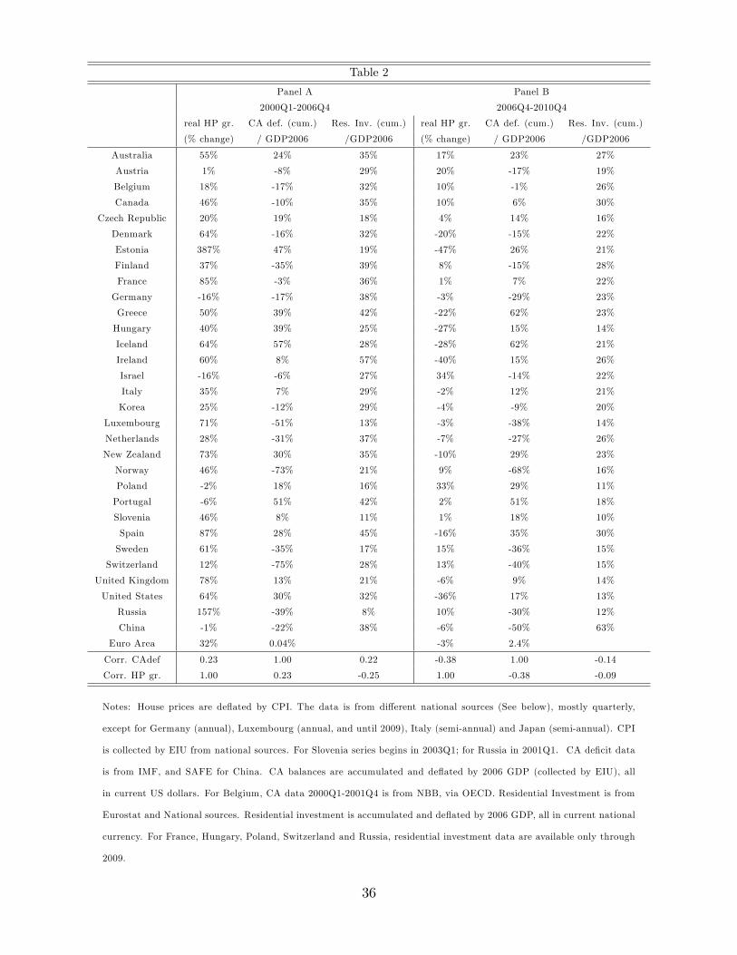
Table 2

Panel A Panel B

2000Q1-2006Q4 2006Q4-2010Q4

real HP gr. CA def. (cum.) Res. Inv. (cum.) real HP gr. CA def. (cum.) Res. Inv. (cum.)

(% change) / GDP2006 /GDP2006 (% change) / GDP2006 /GDP2006

Australia 55% 24% 35% 17% 23% 27%

Austria 1% -8% 29% 20% -17% 19%

Belgium 18% -17% 32% 10% -1% 26%

Canada 46% -10% 35% 10% 6% 30%

Czech Republic 20% 19% 18% 4% 14% 16%

Denmark 64% -16% 32% -20% -15% 22%

Estonia 387% 47% 19% -47% 26% 21%

Finland 37% -35% 39% 8% -15% 28%

France 85% -3% 36% 1% 7% 22%

Germany -16% -17% 38% -3% -29% 23%

Greece 50% 39% 42% -22% 62% 23%

Hungary 40% 39% 25% -27% 15% 14%

Iceland 64% 57% 28% -28% 62% 21%

Ireland 60% 8% 57% -40% 15% 26%

Israel -16% -6% 27% 34% -14% 22%

Italy 35% 7% 29% -2% 12% 21%

Korea 25% -12% 29% -4% -9% 20%

Luxembourg 71% -51% 13% -3% -38% 14%

Netherlands 28% -31% 37% -7% -27% 26%

New Zealand 73% 30% 35% -10% 29% 23%

Norway 46% -73% 21% 9% -68% 16%

Poland -2% 18% 16% 33% 29% 11%

Portugal -6% 51% 42% 2% 51% 18%

Slovenia 46% 8% 11% 1% 18% 10%

Spain 87% 28% 45% -16% 35% 30%

Sweden 61% -35% 17% 15% -36% 15%

Switzerland 12% -75% 28% 13% -40% 15%

United Kingdom 78% 13% 21% -6% 9% 14%

United States 64% 30% 32% -36% 17% 13%

Russia 157% -39% 8% 10% -30% 12%

China -1% -22% 38% -6% -50% 63%

Euro Area 32% 0.04% -3% 2.4%

Corr. CAdef 0.23 1.00 0.22 -0.38 1.00 -0.14

Corr. HP gr. 1.00 0.23 -0.25 1.00 -0.38 -0.09

Notes: House prices are deflated by CPI. The data is from different national sources (See below), mostly quarterly,

except for Germany (annual), Luxembourg (annual, and until 2009), Italy (semi-annual) and Japan (semi-annual). CPI

is collected by EIU from national sources. For Slovenia series begins in 2003Q1; for Russia in 2001Q1. CA deficit data

is from IMF, and SAFE for China. CA balances are accumulated and deflated by 2006 GDP (collected by EIU), all

in current US dollars. For Belgium, CA data 2000Q1-2001Q4 is from NBB, via OECD. Residential Investment is from

Eurostat and National sources. Residential investment is accumulated and deflated by 2006 GDP, all in current national

currency. For France, Hungary, Poland, Switzerland and Russia, residential investment data are available only through

2009.

36

4.1 Regression Analysis

In this section we undertake a basic empirical analysis of correlations among house prices and

other variables. We emphasize that, in presenting these next results, we do not make claims about

causality. Later, focusing on the correlation between credit standards and house prices, we will

provide some additional discussion and evidence on this question.

A few words about the data are in order. First, with regard to an international panel of data,

we are limited to far fewer observations given the availability of bank lending survey data for

non-U.S. countries. These data extend only from 2002:Q4 to 2010:Q4. For this reason we also

look separately at regressions for the U.S. alone, where data reaches back much further, starting

in 1990:Q4. Second, as explained in the Appendix, the data on bank lending standards differs

somewhat by country. When we analyze the U.S. alone, we use the net percentage easing indicator

plotted above. In the other countries the surveys are modeled after the U.S. SLOOS survey, but

the way the survey results are aggregated can differ. For 9 of the 11 countries for which we have

data on credit standards (Austria, Belgium, Euro Area, France, Korea, Portugal, Spain, United

States, Ireland) we have available, or can construct, a diffusion index of credit standards or a scale

transformation thereof (some countries report a mean value indicator—see the appendix—which is a

scale transformation of the diffusion index) with the information reported by the Central Banks.

This diffusion index, however, is not a scale transformation of the net percentage indicator discussed

above, and there are two (Canada and Netherlands) that only report the net percentage indicator.

For the panel regressions that we report on here, we simply use all these data together in one

regression, even though the credit standards measure for two countries (Canada and Netherlands)

are not a scale transformation of the other countries’measures. Results available on request show

that the findings are virtually unchanged if we exclude these two countries. We standardize these

bank lending survey measures, country by country, by subtracting the mean and dividing by the

standard deviation, for the period 2002Q4-2010Q4. This insures that, at least for the 9 countries

for which we have a diffusion index or mean value indicator, the credit supply measure for each

country is in the same units. The Appendix provides more details on the credit supply data by

country.

Third, we use a measure of the change in net foreign holdings of U.S. securities as our main

measure of international capital flows into the U.S. (Although for completeness, we also report

results using the CA deficit.) Recall that annual net foreign holdings estimates are compiled

by the BEA in their international investment data, year-end positions.15 Yet all the rest of our

data are quarterly. Instead of limiting ourselves to annual observations, we therefore form a simple

15As discussed above, these BEA year-end holdings data begin in 1976. This is in contrast to the TIC data onasset holdings which is reported annually only starting in 2002. Thus, the BEA constructs its own estimate ofyear-end positions prior to 2002 using as raw inputs the TIC flows data and the periodic TIC benchmark surveysof holdings. The BEA year-end data are located at http://www.bea.gov/international/xls/intinv10_t2.xls

37

estimate of the quarter-end net foreign liability position of the U.S. in total securities, by employing

a methodology to interpolate between the year-end positions, taking into account the quarterly

transactions data in these same securities.16 The procedure is as follows.

Let nhQ4 be the value of net foreign holdings of total securities observed at the end of quarter

Q4 of a given year, where net foreign holdings are defined as foreign holdings of U.S. securities

minus U.S. holdings of foreign securities. These data are available from the BEA year-end positions

table. Let n̂hq be an estimate that we will form of the value of these net foreign holdings at the end

of quarter q in that same year. Let ntq be net transactions in those securities during that quarter,

where net transactions are net foreign purchases (gross foreign purchases less gross foreign sales)

of U.S. owned securities minus U.S. net purchases (gross U.S. purchases less gross U.S. sales) of

foreign owned securities. These data are available from the BEA international transactions table.

To obtain estimates of quarterly holdings for the three quarters within a year, we accumulate

according to

n̂hq = n̂hq−1 + ntq + adjq

where

adjq = gapQ4 ∗ wq,Q4

wq,Q4 ≡|ntq|

3∑k=0

|ntQ4−k|

gapQ4 ≡ (nhQ4 − nhQ4−4)−3∑k=0

ntQ4−k.

The above recursion ensures that our estimate of the holdings at the end of Q4 of a given year,

n̂hQ4, is equal to the recorded value from the annual holdings data, nhQ4. For all other quarters

within a year, the above recursion forms an estimate of holdings at the end of the quarter, which is

equal to the estimated net holdings from last quarter, plus the net transactions in that quarter, plus

an adjustment. The adjustment is equal to the gap between the change in measured holdings from

the year in which the quarter resides and the previous year and the cumulation of all the quarterly

transactions over the year, times a weight, where the weight is given by that quarter’s value of net

transactions relative to the value over the entire year. Thus, quarters for which net transactions

were higher in absolute value receive a greater weight in the adjustment. Notice that, in the absence

of any valuation adjustments, the cumulation of all the quarterly transactions over the year would

equal the total change in net foreign holdings or year-end positions. The observed change in year-

end positions takes into account the valuation changes, and gapQ4 is the difference between the

observed change in year-end positions and the cumulation of the quarterly transactions. Thus,

16The data on international transactions in financial securities are in the balance of payments dataset, found athttp://www.bea.gov/international/xls/table1.xls.

38

roughly speaking, the adjustment adjq captures the pure valuation effects that are not reflected in

the cumulation of transactions but are reflected in the total change in net foreign holdings. The

weights wq,Q4 give quarters with a larger value of transactions more weight in the adjustment. We

now present results from a regression analysis using these and other data.

We begin with evidence from the panel of 11 countries mentioned above (Austria, Belgium,

Canada, Euro Area, France, Korea, Netherlands Portugal, Spain, United States, Ireland). For these

countries, we have quarterly observations from 2002:Q4 to 2010:Q4 on real house price growth, the

current account deficit and credit standards. The variable CS in these regressions is a diffusion

index measure that, when increased, indicates an easing of credit standards. A detailed description

of all of these data, including data sources, is given in the Appendix. Table 3 reports the results

of a panel fixed-effects regression of real house price growth on the current account, CS, and

interactions of these variables. The variable CAdef/GDP is the current account deficit, divided

by the country’s GDP.

Table 3 shows that CAdef/GDP bears a negative relation to contemporaneous real house price

growth, though it is not statistically significant.17 The credit standard measure CS is statistically

significant, and an increase in CS leads to an increase in real house price growth (row 2). Row 3

shows that CS remains the only significant determinant of house price growth when both variables

are included, while rows 4 and 5 document some interaction effects: countries and time periods in

which there was an increase in credit supply experienced a larger increase in house price growth if

they also ran current account deficits. But, controlling for this, CAdef/GDP has a statistically

insignificant marginal effect on house price growth (row 4), while CS by itself has a strongly

significant marginal effect (row 5). The R2 statistics range from 6 to 9 percent whenever CStis included in the regression, either by itself or interactively with CAdef/GDP. To interpret the

magnitudes of the coeffi cients on CS, recall that this variables is standardized, so a one-unit

increase in this measure implies a one standard deviation increase around its mean. The coeffi cient

is 0.005, which implies that a one-standard deviation increase in CS leads to a 50 basis point

rise in quarterly real house price growth, roughly a 2% rise at an annual rate. This increase

represents about one-quarter of a one-standard deviation change in quarterly U.S. real house price

growth (2.0%).These results provide little support for the hypothesis that capital inflows played

an important role in driving the changes in house prices internationally over the recent boom-bust

period.

17We use the Driscoll and Kraay (1998) consistent covariance-matrix estimates to produce heteroscedasticityconsistent standard errors that are robust to general forms of autocorrelation and cross-sectional (spatial) correlationbetween the residuals.

39

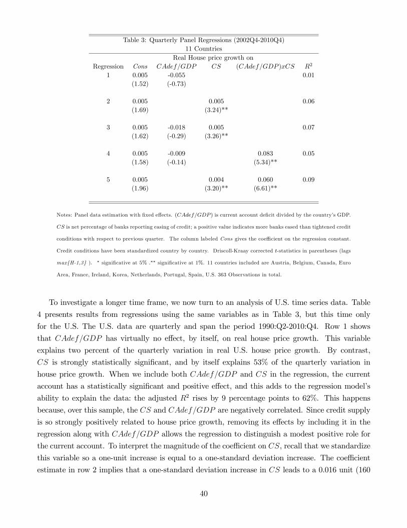
Table 3: Quarterly Panel Regressions (2002Q4-2010Q4)11 Countries

Real House price growth onRegression Cons CAdef/GDP CS (CAdef/GDP )xCS R2

1 0.005 -0.055 0.01(1.52) (-0.73)

2 0.005 0.005 0.06(1.69) (3.24)**

3 0.005 -0.018 0.005 0.07(1.62) (-0.29) (3.26)**

4 0.005 -0.009 0.083 0.05(1.58) (-0.14) (5.34)**

5 0.005 0.004 0.060 0.09(1.96) (3.20)** (6.61)**

Notes: Panel data estimation with fixed effects. (CAdef/GDP ) is current account deficit divided by the country’s GDP.

CS is net percentage of banks reporting easing of credit; a positive value indicates more banks eased than tightened credit

conditions with respect to previous quarter. The column labeled Cons gives the coeffi cient on the regression constant.

Credit conditions have been standardized country by country. Driscoll-Kraay corrected t-statistics in parentheses (lags

max{H-1,3} ). ∗ significative at 5% .∗∗ significative at 1%. 11 countries included are Austria, Belgium, Canada, Euro

Area, France, Ireland, Korea, Netherlands, Portugal, Spain, U.S. 363 Observations in total.

To investigate a longer time frame, we now turn to an analysis of U.S. time series data. Table

4 presents results from regressions using the same variables as in Table 3, but this time only

for the U.S. The U.S. data are quarterly and span the period 1990:Q2-2010:Q4. Row 1 shows

that CAdef/GDP has virtually no effect, by itself, on real house price growth. This variable

explains two percent of the quarterly variation in real U.S. house price growth. By contrast,

CS is strongly statistically significant, and by itself explains 53% of the quarterly variation in

house price growth. When we include both CAdef/GDP and CS in the regression, the current

account has a statistically significant and positive effect, and this adds to the regression model’s

ability to explain the data: the adjusted R2 rises by 9 percentage points to 62%. This happens

because, over this sample, the CS and CAdef/GDP are negatively correlated. Since credit supply

is so strongly positively related to house price growth, removing its effects by including it in the

regression along with CAdef/GDP allows the regression to distinguish a modest positive role for

the current account. To interpret the magnitude of the coeffi cient on CS, recall that we standardize

this variable so a one-unit increase is equal to a one-standard deviation increase. The coeffi cient

estimate in row 2 implies that a one-standard deviation increase in CS leads to a 0.016 unit (160

40

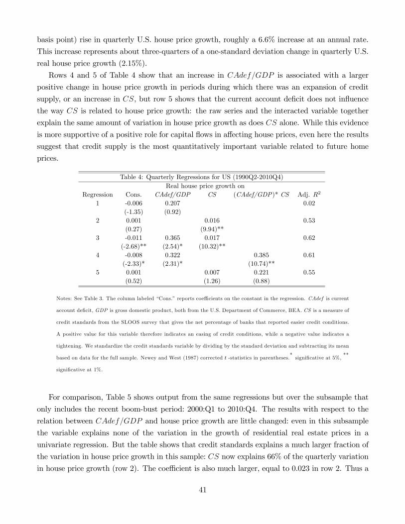
basis point) rise in quarterly U.S. house price growth, roughly a 6.6% increase at an annual rate.

This increase represents about three-quarters of a one-standard deviation change in quarterly U.S.

real house price growth (2.15%).

Rows 4 and 5 of Table 4 show that an increase in CAdef/GDP is associated with a larger

positive change in house price growth in periods during which there was an expansion of credit

supply, or an increase in CS, but row 5 shows that the current account deficit does not influence

the way CS is related to house price growth: the raw series and the interacted variable together

explain the same amount of variation in house price growth as does CS alone. While this evidence

is more supportive of a positive role for capital flows in affecting house prices, even here the results

suggest that credit supply is the most quantitatively important variable related to future home

prices.

Table 4: Quarterly Regressions for US (1990Q2-2010Q4)Real house price growth on

Regression Cons. CAdef/GDP CS (CAdef/GDP)* CS Adj. R2

1 -0.006 0.207 0.02(-1.35) (0.92)

2 0.001 0.016 0.53(0.27) (9.94)**

3 -0.011 0.365 0.017 0.62(-2.68)** (2.54)* (10.32)**

4 -0.008 0.322 0.385 0.61(-2.33)* (2.31)* (10.74)**

5 0.001 0.007 0.221 0.55(0.52) (1.26) (0.88)

Notes: See Table 3. The column labeled “Cons.”reports coeffi cients on the constant in the regression. CAdef is current

account deficit, GDP is gross domestic product, both from the U.S. Department of Commerce, BEA. CS is a measure of

credit standards from the SLOOS survey that gives the net percentage of banks that reported easier credit conditions.

A positive value for this variable therefore indicates an easing of credit conditions, while a negative value indicates a

tightening. We standardize the credit standards variable by dividing by the standard deviation and subtracting its mean

based on data for the full sample. Newey and West (1987) corrected t -statistics in parentheses.* significative at 5%, **

significative at 1%.

For comparison, Table 5 shows output from the same regressions but over the subsample that

only includes the recent boom-bust period: 2000:Q1 to 2010:Q4. The results with respect to the

relation between CAdef/GDP and house price growth are little changed: even in this subsample

the variable explains none of the variation in the growth of residential real estate prices in a

univariate regression. But the table shows that credit standards explains a much larger fraction of

the variation in house price growth in this sample: CS now explains 66% of the quarterly variation

in house price growth (row 2). The coeffi cient is also much larger, equal to 0.023 in row 2. Thus a

41

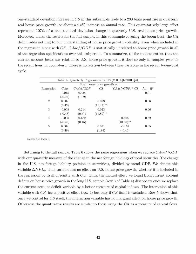
one-standard deviation increase in CS in this subsample leads to a 230 basis point rise in quarterly

real house price growth, or about a 9.5% increase an annual rate. This quantitatively large effect

represents 107% of a one-standard deviation change in quarterly U.S. real house price growth.

Moreover, unlike the results for the full sample, in this subsample covering the boom-bust, the CA

deficit adds nothing to our understanding of house price growth volatility, even when included in

the regression along with CS. CAdef/GDP is statistically unrelated to house price growth in all

of the regression specifications over this subperiod. To summarize, to the modest extent that the

current account bears any relation to U.S. house price growth, it does so only in samples prior to

the recent housing boom-bust. There is no relation between these variables in the recent boom-bust

cycle.

Table 5: Quarterly Regressions for US (2000:Q1-2010:Q4)Real house price growth on

Regression Cons CAdef/GDP CS (CAdef/GDP)* CS Adj. R2

1 -0.018 0.435 0.01(-0.96) (1.02)

2 0.002 0.023 0.66(0.43) (11.43)**

3 -0.008 0.214 0.023 0.66(-0.48) (0.57) (11.89)**

4 -0.008 0.189 0.465 0.62(-0.40) (0.45) (10.60)**

5 0.002 0.031 -0.162 0.65(0.46) (1.84) (-0.46)

Notes: See Table 4.

Returning to the full sample, Table 6 shows the same regressions when we replace CAdef/GDP

with our quarterly measure of the change in the net foreign holdings of total securities (the change

in the U.S. net foreign liability position in securities), divided by trend GDP. We denote this

variable ∆NFLt. This variable has no effect on U.S. house price growth, whether it is included in

the regression by itself or jointly with CSt. Thus, the modest effect we found from current account

deficits on house price growth in the long U.S. sample (row 3 of Table 4) disappears once we replace

the current account deficit variable by a better measure of capital inflows. The interaction of this

variable with CSt has a positive effect (row 4) but only if CS itself is excluded. Row 5 shows that,

once we control for CS itself, the interaction variable has no marginal affect on house price growth.

Otherwise the quantitative results are similar to those using the CA as a measure of capital flows.

42

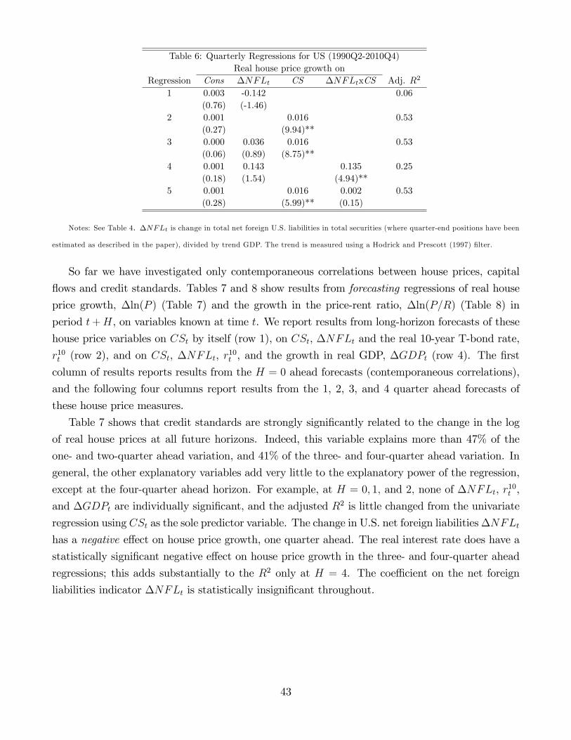
Table 6: Quarterly Regressions for US (1990Q2-2010Q4)Real house price growth on

Regression Cons ∆NFLt CS ∆NFLtxCS Adj. R2

1 0.003 -0.142 0.06(0.76) (-1.46)

2 0.001 0.016 0.53(0.27) (9.94)**

3 0.000 0.036 0.016 0.53(0.06) (0.89) (8.75)**

4 0.001 0.143 0.135 0.25(0.18) (1.54) (4.94)**

5 0.001 0.016 0.002 0.53(0.28) (5.99)** (0.15)

Notes: See Table 4. ∆NFLt is change in total net foreign U.S. liabilities in total securities (where quarter-end positions have been

estimated as described in the paper), divided by trend GDP. The trend is measured using a Hodrick and Prescott (1997) filter.

So far we have investigated only contemporaneous correlations between house prices, capital

flows and credit standards. Tables 7 and 8 show results from forecasting regressions of real house

price growth, ∆ln(P ) (Table 7) and the growth in the price-rent ratio, ∆ln(P/R) (Table 8) in

period t+H, on variables known at time t. We report results from long-horizon forecasts of these

house price variables on CSt by itself (row 1), on CSt, ∆NFLt and the real 10-year T-bond rate,

r10t (row 2), and on CSt, ∆NFLt, r10

t , and the growth in real GDP, ∆GDPt (row 4). The first

column of results reports results from the H = 0 ahead forecasts (contemporaneous correlations),

and the following four columns report results from the 1, 2, 3, and 4 quarter ahead forecasts of

these house price measures.

Table 7 shows that credit standards are strongly significantly related to the change in the log

of real house prices at all future horizons. Indeed, this variable explains more than 47% of the

one- and two-quarter ahead variation, and 41% of the three- and four-quarter ahead variation. In

general, the other explanatory variables add very little to the explanatory power of the regression,

except at the four-quarter ahead horizon. For example, at H = 0, 1, and 2, none of ∆NFLt, r10t ,

and ∆GDPt are individually significant, and the adjusted R2 is little changed from the univariate

regression using CSt as the sole predictor variable. The change in U.S. net foreign liabilities∆NFLt

has a negative effect on house price growth, one quarter ahead. The real interest rate does have a

statistically significant negative effect on house price growth in the three- and four-quarter ahead

regressions; this adds substantially to the R2 only at H = 4. The coeffi cient on the net foreign

liabilities indicator ∆NFLt is statistically insignificant throughout.

43

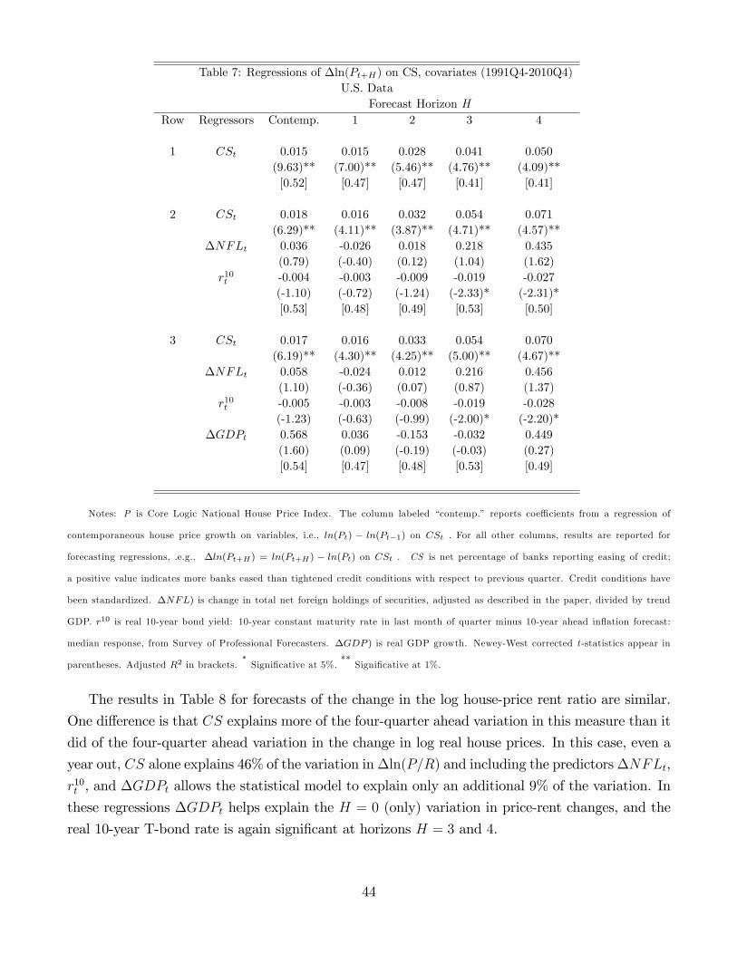
Table 7: Regressions of ∆ln(Pt+H) on CS, covariates (1991Q4-2010Q4)U.S. Data

Forecast Horizon HRow Regressors Contemp. 1 2 3 4

1 CSt 0.015 0.015 0.028 0.041 0.050(9.63)** (7.00)** (5.46)** (4.76)** (4.09)**[0.52] [0.47] [0.47] [0.41] [0.41]

2 CSt 0.018 0.016 0.032 0.054 0.071(6.29)** (4.11)** (3.87)** (4.71)** (4.57)**

∆NFLt 0.036 -0.026 0.018 0.218 0.435(0.79) (-0.40) (0.12) (1.04) (1.62)

r10t -0.004 -0.003 -0.009 -0.019 -0.027(-1.10) (-0.72) (-1.24) (-2.33)* (-2.31)*[0.53] [0.48] [0.49] [0.53] [0.50]

3 CSt 0.017 0.016 0.033 0.054 0.070(6.19)** (4.30)** (4.25)** (5.00)** (4.67)**

∆NFLt 0.058 -0.024 0.012 0.216 0.456(1.10) (-0.36) (0.07) (0.87) (1.37)

r10t -0.005 -0.003 -0.008 -0.019 -0.028(-1.23) (-0.63) (-0.99) (-2.00)* (-2.20)*

∆GDPt 0.568 0.036 -0.153 -0.032 0.449(1.60) (0.09) (-0.19) (-0.03) (0.27)[0.54] [0.47] [0.48] [0.53] [0.49]

Notes: P is Core Logic National House Price Index. The column labeled “contemp.” reports coeffi cients from a regression of

contemporaneous house price growth on variables, i.e., ln(Pt) − ln(Pt−1) on CSt . For all other columns, results are reported for

forecasting regressions, .e.g., ∆ln(Pt+H) = ln(Pt+H) − ln(Pt) on CSt . CS is net percentage of banks reporting easing of credit;

a positive value indicates more banks eased than tightened credit conditions with respect to previous quarter. Credit conditions have

been standardized. ∆NFL) is change in total net foreign holdings of securities, adjusted as described in the paper, divided by trend

GDP. r10 is real 10-year bond yield: 10-year constant maturity rate in last month of quarter minus 10-year ahead inflation forecast:

median response, from Survey of Professional Forecasters. ∆GDP ) is real GDP growth. Newey-West corrected t -statistics appear in

parentheses. Adjusted R2 in brackets.∗Significative at 5%. ** Significative at 1%.

The results in Table 8 for forecasts of the change in the log house-price rent ratio are similar.

One difference is that CS explains more of the four-quarter ahead variation in this measure than it

did of the four-quarter ahead variation in the change in log real house prices. In this case, even a

year out, CS alone explains 46% of the variation in∆ln(P/R) and including the predictors∆NFLt,

r10t , and ∆GDPt allows the statistical model to explain only an additional 9% of the variation. In

these regressions ∆GDPt helps explain the H = 0 (only) variation in price-rent changes, and the

real 10-year T-bond rate is again significant at horizons H = 3 and 4.

44

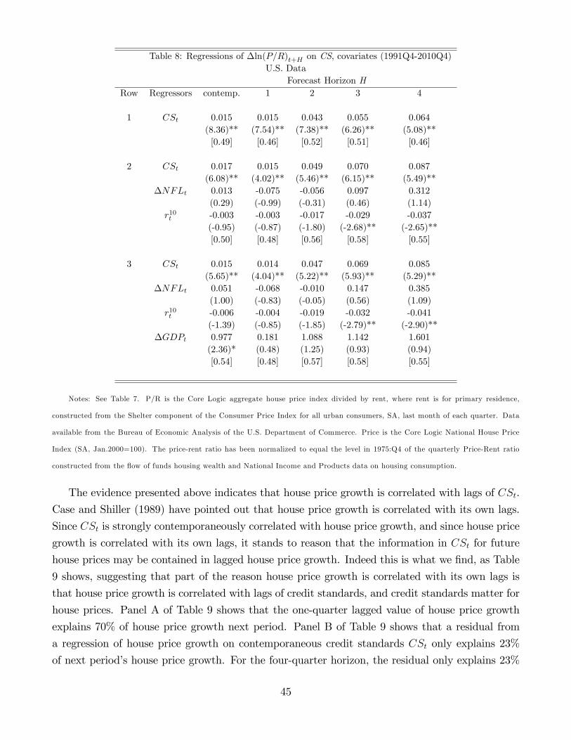
Table 8: Regressions of ∆ln(P/R)t+H on CS, covariates (1991Q4-2010Q4)U.S. Data

Forecast Horizon HRow Regressors contemp. 1 2 3 4

1 CSt 0.015 0.015 0.043 0.055 0.064(8.36)** (7.54)** (7.38)** (6.26)** (5.08)**[0.49] [0.46] [0.52] [0.51] [0.46]

2 CSt 0.017 0.015 0.049 0.070 0.087(6.08)** (4.02)** (5.46)** (6.15)** (5.49)**

∆NFLt 0.013 -0.075 -0.056 0.097 0.312(0.29) (-0.99) (-0.31) (0.46) (1.14)

r10t -0.003 -0.003 -0.017 -0.029 -0.037(-0.95) (-0.87) (-1.80) (-2.68)** (-2.65)**[0.50] [0.48] [0.56] [0.58] [0.55]

3 CSt 0.015 0.014 0.047 0.069 0.085(5.65)** (4.04)** (5.22)** (5.93)** (5.29)**

∆NFLt 0.051 -0.068 -0.010 0.147 0.385(1.00) (-0.83) (-0.05) (0.56) (1.09)

r10t -0.006 -0.004 -0.019 -0.032 -0.041(-1.39) (-0.85) (-1.85) (-2.79)** (-2.90)**

∆GDPt 0.977 0.181 1.088 1.142 1.601(2.36)* (0.48) (1.25) (0.93) (0.94)[0.54] [0.48] [0.57] [0.58] [0.55]

Notes: See Table 7. P/R is the Core Logic aggregate house price index divided by rent, where rent is for primary residence,

constructed from the Shelter component of the Consumer Price Index for all urban consumers, SA, last month of each quarter. Data

available from the Bureau of Economic Analysis of the U.S. Department of Commerce. Price is the Core Logic National House Price

Index (SA, Jan.2000=100). The price-rent ratio has been normalized to equal the level in 1975:Q4 of the quarterly Price-Rent ratio

constructed from the flow of funds housing wealth and National Income and Products data on housing consumption.

The evidence presented above indicates that house price growth is correlated with lags of CSt.

Case and Shiller (1989) have pointed out that house price growth is correlated with its own lags.

Since CSt is strongly contemporaneously correlated with house price growth, and since house price

growth is correlated with its own lags, it stands to reason that the information in CSt for future

house prices may be contained in lagged house price growth. Indeed this is what we find, as Table

9 shows, suggesting that part of the reason house price growth is correlated with its own lags is

that house price growth is correlated with lags of credit standards, and credit standards matter for

house prices. Panel A of Table 9 shows that the one-quarter lagged value of house price growth

explains 70% of house price growth next period. Panel B of Table 9 shows that a residual from

a regression of house price growth on contemporaneous credit standards CSt only explains 23%

of next period’s house price growth. For the four-quarter horizon, the residual only explains 23%

45

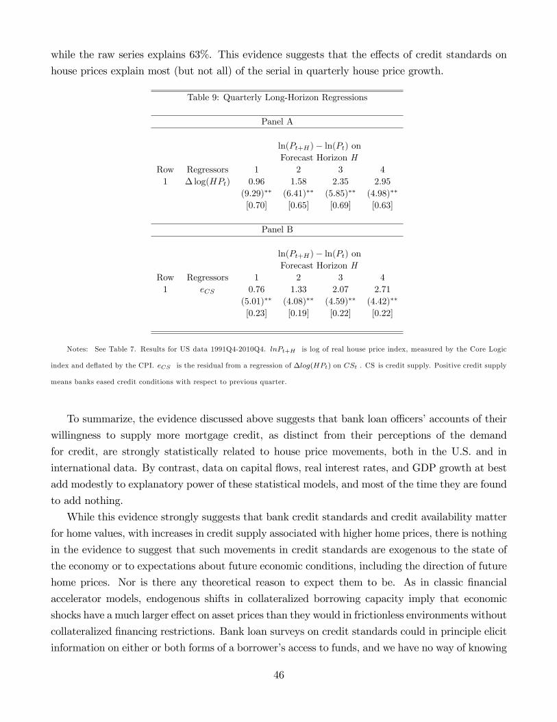
while the raw series explains 63%. This evidence suggests that the effects of credit standards on

house prices explain most (but not all) of the serial in quarterly house price growth.

Table 9: Quarterly Long-Horizon Regressions

Panel A

ln(Pt+H)− ln(Pt) onForecast Horizon H

Row Regressors 1 2 3 41 ∆ log(HPt) 0.96 1.58 2.35 2.95

(9.29)∗∗ (6.41)∗∗ (5.85)∗∗ (4.98)∗∗

[0.70] [0.65] [0.69] [0.63]

Panel B

ln(Pt+H)− ln(Pt) onForecast Horizon H

Row Regressors 1 2 3 41 eCS 0.76 1.33 2.07 2.71

(5.01)∗∗ (4.08)∗∗ (4.59)∗∗ (4.42)∗∗

[0.23] [0.19] [0.22] [0.22]

Notes: See Table 7. Results for US data 1991Q4-2010Q4. lnPt+H is log of real house price index, measured by the Core Logic

index and deflated by the CPI. eCS is the residual from a regression of ∆log(HPt) on CSt . CS is credit supply. Positive credit supply

means banks eased credit conditions with respect to previous quarter.

To summarize, the evidence discussed above suggests that bank loan offi cers’accounts of their

willingness to supply more mortgage credit, as distinct from their perceptions of the demand

for credit, are strongly statistically related to house price movements, both in the U.S. and in

international data. By contrast, data on capital flows, real interest rates, and GDP growth at best

add modestly to explanatory power of these statistical models, and most of the time they are found

to add nothing.

While this evidence strongly suggests that bank credit standards and credit availability matter

for home values, with increases in credit supply associated with higher home prices, there is nothing

in the evidence to suggest that such movements in credit standards are exogenous to the state of

the economy or to expectations about future economic conditions, including the direction of future

home prices. Nor is there any theoretical reason to expect them to be. As in classic financial

accelerator models, endogenous shifts in collateralized borrowing capacity imply that economic

shocks have a much larger effect on asset prices than they would in frictionless environments without

collateralized financing restrictions. Bank loan surveys on credit standards could in principle elicit

information on either or both forms of a borrower’s access to funds, and we have no way of knowing

46

from the survey questions how much of any given change in standards is represented by one or the

other. In our view, either of these represents a movement in credit availability, and both could be

important for home prices.

Still, don’t endogenous movements in credit supply raise a question of causality? If credit

standards move in response to changing economic conditions, which in turn alter expectations of

future home price movements, then how do we rule out the possibility that (current and future)

home prices affect credit availability rather than the other way around? The answer, we argue, is

that we don’t rule this out nor should we seek to, since the direction of causality is not central for

the question of whether credit availability plays a role in driving asset price fluctuations. A natural

benchmark is a complete markets environment, where borrowing constraints and transactions costs

play no role in the equilibrium allocations. Indeed, it’s hard to understand why credit standards

would be correlated at all with asset values in such an environment. With incomplete markets,

credit availability can have a large dynamic impact on asset prices even if fluctuations in that

availability are completely endogenous. From this perspective, as long as we have a clean measure

of credit supply, as distinct from credit demand, any correlation of credit supply with asset prices

is of relevance for the question of whether credit supply matters for asset prices.

That said, we do want to distinguish movements in credit supply from movements in credit

demand. The SLOOS survey explicitly asks banks to do so, but their may be some residual

correlation between the two. Moreover, it is of some interest to ask whether, as a factual matter,

the credit supply measure that we study has an exogenous component that still affects house prices

once we control for expectations about future economic conditions.

Table 10 presents some evidence related to these questions. Instead of using the raw credit

supply CSt series, for these results we first regress it on the SLOOS survey’s measure of credit

demand (the net percentage of banks reporting higher credit demand), and take the residual of

this regression εCD,t, as a measure of credit supply. (After obtaining this residual we standardize

it so as to give it the same units the raw measure used previously had.)We also replace current

GDP growth from the regressions above, with the expected GDP growth rate for the year ahead,

∆GDPt→t+4, as measured by the Survey of Professional Forecasters (SPF) median forecast. In

these regressions, we continue to use our measure of capital inflows ∆NFLt and the real 10-year

T-bond rate r10t as additional explanatory variables. Notice that r10

t is itself a forward looking

variable since it equals the nominal 10-year T-bond rate minus the expected 10-year inflation rate

(also from the SPF, median forecast). Once we include these forecasts of future economic activity

as additional predictor variables, any remaining role for our residual credit supply measure εCD,tin explaining house price movements must be independent of such expectations.

47

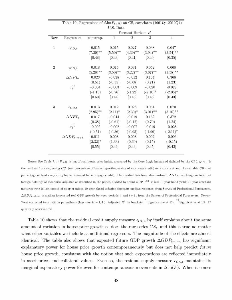
Table 10: Regressions of ∆ln(Pt+H) on CS, covariates (1991Q4-2010Q4)U.S. Data

Forecast Horizon HRow Regressors contemp. 1 2 3 4

1 εCD,t 0.015 0.015 0.027 0.038 0.047(7.20)** (5.50)** (4.39)** (3.94)** (3.54)**[0.48] [0.43] [0.41] [0.40] [0.35]

2 εCD,t 0.018 0.015 0.031 0.052 0.068(5.28)** (3.50)** (3.22)** (3.67)** (3.58)**

∆NFLt 0.023 -0.038 -0.012 0.164 0.368(0.51) (-0.55) (-0.08) (0.71) (1.23)

r10t -0.004 -0.003 -0.009 -0.020 -0.028(-1.13) (-0.76) (-1.22) (-2.10)* (-2.08)*[0.50] [0.44] [0.43] [0.46] [0.43]

3 εCD,t 0.013 0.012 0.028 0.051 0.070(2.95)** (2.11)* (2.30)* (3.01)** (3.10)**

∆NFLt 0.017 -0.044 -0.019 0.162 0.372(0.38) (-0.61) (-0.12) (0.70) (1.24)

r10t -0.002 -0.002 -0.007 -0.019 -0.028(-0.51) (-0.36) (-0.95) (-1.99) (-2.11)*

∆GDPt→t+4 0.011 0.008 0.008 0.002 -0.003(2.32)* (1.33) (0.69) (0.15) (-0.15)[0.55] [0.46] [0.43] [0.45] [0.42]

Notes: See Table 7. lnPt+H is log of real house price index, measured by the Core Logic index and deflated by the CPI. eCD,t is

the residual from regressing CS (net percentage of banks reporting easing of mortgage credit) on a constant and the variable CD (net

percentage of banks reporting higher demand for mortgage credit). The residual has been standardized. ∆NFL is change in total net

foreign holdings of securities, adjusted as described in the paper, divided by trend GDP. r10 is real 10-year bond yield: 10-year constant

maturity rate in last month of quarter minus 10-year ahead inflation forecast: median response, from Survey of Professional Forecasters.

∆GDPt→t+4 is median forecasted real GDP growth between periods t and t+ 4 , from the Survey of Professional Forecasters. Newey-

West corrected t-statistic in parenthesis (lags maxH − 1, 4 ). Adjusted R2 in brackets.*Significative at 5%. **Significative at 1%. 77

quarterly observations.

Table 10 shows that the residual credit supply measure εCD,t by itself explains about the same

amount of variation in house price growth as does the raw series CSt, and this is true no matter

what other variables we include as additional regressors. The magnitude of the effects are almost

identical. The table also shows that expected future GDP growth ∆GDPt→t+4 has significant

explanatory power for house price growth contemporaneously but does not help predict future

house price growth, consistent with the notion that such expectations are reflected immediately

in asset prices and collateral values. Even so, the residual supply measure εCD,t maintains its

marginal explanatory power for even for contemporaneous movements in ∆ ln(P ). When it comes

48

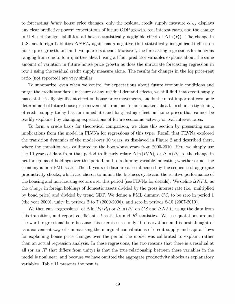
to forecasting future house price changes, only the residual credit supply measure εCD,t displays

any clear predictive power: expectations of future GDP growth, real interest rates, and the change

in U.S. net foreign liabilities, all have a statistically negligible effect of ∆ ln (Pt). The change in

U.S. net foreign liabilities ∆NFLt again has a negative (but statistically insignificant) effect on

house price growth, one and two quarters ahead. Moreover, the forecasting regressions for horizons

ranging from one to four quarters ahead using all four predictor variables explains about the same

amount of variation in future house price growth as does the univariate forecasting regression in

row 1 using the residual credit supply measure alone. The results for changes in the log price-rent

ratio (not reported) are very similar.

To summarize, even when we control for expectations about future economic conditions and

purge the credit standards measure of any residual demand effects, we still find that credit supply

has a statistically significant effect on house price movements, and is the most important economic

determinant of future house price movements from one to four quarters ahead. In short, a tightening

of credit supply today has an immediate and long-lasting effect on home prices that cannot be

readily explained by changing expectations of future economic activity or real interest rates.

To form a crude basis for theoretical comparison, we close this section by presenting some

implications from the model in FLVNa for regressions of this type. Recall that FLVNa explored

the transition dynamics of the model over 10 years, as displayed in Figure 2 and described there,

where the transition was calibrated to the boom-bust years from 2000-2010. Here we simply use

the 10 years of data from that period to linearly relate ∆ ln (P/R)t or ∆ ln (Pt) to the change in

net foreign asset holdings over this period, and to a dummy variable indicating whether or not the

economy is in a FML state. The 10 years of data are also influenced by the sequence of aggregate

productivity shocks, which are chosen to mimic the business cycle and the relative performance of

the housing and non-housing sectors over this period (see FLVNa for details). We define ∆NFLt as

the change in foreign holdings of domestic assets divided by the gross interest rate (i.e., multiplied

by bond price) and divided by trend GDP. We define a FML dummy, CS, to be zero in period 1

(the year 2000), unity in periods 2 to 7 (2000-2006), and zero in periods 8-10 (2007-2010).

We then run “regressions”of ∆ ln (Pt/Rt) or ∆ ln (Pt) on CS and ∆NFLt using the data from

this transition, and report coeffi cients, t-statistics and R2 statistics. We use quotations around

the word ‘regressions’here because this exercise uses only 10 observations and is best thought of

as a convenient way of summarizing the marginal contributions of credit supply and capital flows

for explaining house price changes over the period the model was calibrated to explain, rather

than an actual regression analysis. In these regressions, the two reasons that there is a residual at

all (or an R2 that differs from unity) is that the true relationship between these variables in the

model is nonlinear, and because we have omitted the aggregate productivity shocks as explanatory

variables. Table 11 presents the results.

49

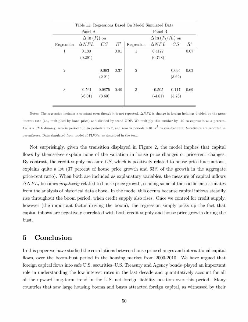
Table 11: Regressions Based On Model Simulated Data

Panel A Panel B

∆ ln (Pt) on ∆ ln (Pt/Rt) on

Regression ∆NFL CS R2 Regression ∆NFL CS R2

1 0.130 0.01 1 0.4177 0.07

(0.291) (0.748)

2 0.063 0.37 2 0.095 0.63

(2.21) (3.62)

3 -0.561 0.0875 0.48 3 -0.505 0.117 0.69

(-6.01) (3.60) (-4.01) (5.73)

Notes: The regression includes a constant even though it is not reported. ∆NFL is change in foreign holdings divided by the gross

interest rate (i.e., multiplied by bond price) and divided by trend GDP. We multiply this number by 100 to express it as a percent.

CS is a FML dummy, zero in period 1, 1 in periods 2 to 7, and zero in periods 8-10. rf is risk-free rate. t -statistics are reported in

parentheses. Data simulated from model of FLVNa, as described in the text.

Not surprisingly, given the transition displayed in Figure 2, the model implies that capital

flows by themselves explain none of the variation in house price changes or price-rent changes.

By contrast, the credit supply measure CS, which is positively related to house price fluctuations,

explains quite a lot (37 percent of house price growth and 63% of the growth in the aggregate

price-rent ratio). When both are included as explanatory variables, the measure of capital inflows

∆NFLt becomes negatively related to house price growth, echoing some of the coeffi cient estimates

from the analysis of historical data above. In the model this occurs because capital inflows steadily

rise throughout the boom period, when credit supply also rises. Once we control for credit supply,

however (the important factor driving the boom), the regression simply picks up the fact that

capital inflows are negatively correlated with both credit supply and house price growth during the

bust.

5 Conclusion

In this paper we have studied the correlations between house price changes and international capital

flows, over the boom-bust period in the housing market from 2000-2010. We have argued that

foreign capital flows into safe U.S. securities—U.S. Treasury and Agency bonds—played an important

role in understanding the low interest rates in the last decade and quantitatively account for all

of the upward long-term trend in the U.S. net foreign liability position over this period. Many

countries that saw large housing booms and busts attracted foreign capital, as witnessed by their

50

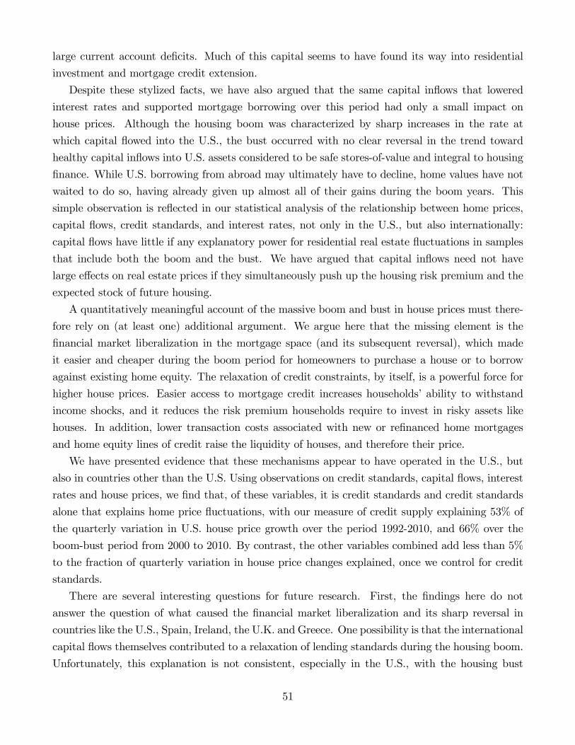
large current account deficits. Much of this capital seems to have found its way into residential

investment and mortgage credit extension.

Despite these stylized facts, we have also argued that the same capital inflows that lowered

interest rates and supported mortgage borrowing over this period had only a small impact on

house prices. Although the housing boom was characterized by sharp increases in the rate at

which capital flowed into the U.S., the bust occurred with no clear reversal in the trend toward

healthy capital inflows into U.S. assets considered to be safe stores-of-value and integral to housing

finance. While U.S. borrowing from abroad may ultimately have to decline, home values have not

waited to do so, having already given up almost all of their gains during the boom years. This

simple observation is reflected in our statistical analysis of the relationship between home prices,

capital flows, credit standards, and interest rates, not only in the U.S., but also internationally:

capital flows have little if any explanatory power for residential real estate fluctuations in samples

that include both the boom and the bust. We have argued that capital inflows need not have

large effects on real estate prices if they simultaneously push up the housing risk premium and the

expected stock of future housing.

A quantitatively meaningful account of the massive boom and bust in house prices must there-

fore rely on (at least one) additional argument. We argue here that the missing element is the

financial market liberalization in the mortgage space (and its subsequent reversal), which made

it easier and cheaper during the boom period for homeowners to purchase a house or to borrow

against existing home equity. The relaxation of credit constraints, by itself, is a powerful force for

higher house prices. Easier access to mortgage credit increases households’ability to withstand

income shocks, and it reduces the risk premium households require to invest in risky assets like

houses. In addition, lower transaction costs associated with new or refinanced home mortgages

and home equity lines of credit raise the liquidity of houses, and therefore their price.

We have presented evidence that these mechanisms appear to have operated in the U.S., but

also in countries other than the U.S. Using observations on credit standards, capital flows, interest

rates and house prices, we find that, of these variables, it is credit standards and credit standards

alone that explains home price fluctuations, with our measure of credit supply explaining 53% of

the quarterly variation in U.S. house price growth over the period 1992-2010, and 66% over the

boom-bust period from 2000 to 2010. By contrast, the other variables combined add less than 5%

to the fraction of quarterly variation in house price changes explained, once we control for credit

standards.

There are several interesting questions for future research. First, the findings here do not

answer the question of what caused the financial market liberalization and its sharp reversal in

countries like the U.S., Spain, Ireland, the U.K. and Greece. One possibility is that the international

capital flows themselves contributed to a relaxation of lending standards during the housing boom.

Unfortunately, this explanation is not consistent, especially in the U.S., with the housing bust

51

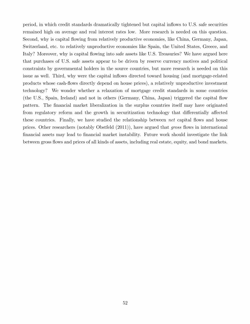
period, in which credit standards dramatically tightened but capital inflows to U.S. safe securities

remained high on average and real interest rates low. More research is needed on this question.

Second, why is capital flowing from relatively productive economies, like China, Germany, Japan,

Switzerland, etc. to relatively unproductive economies like Spain, the United States, Greece, and

Italy? Moreover, why is capital flowing into safe assets like U.S. Treasuries? We have argued here

that purchases of U.S. safe assets appear to be driven by reserve currency motives and political

constraints by governmental holders in the source countries, but more research is needed on this

issue as well. Third, why were the capital inflows directed toward housing (and mortgage-related

products whose cash-flows directly depend on house prices), a relatively unproductive investment

technology? We wonder whether a relaxation of mortgage credit standards in some countries

(the U.S., Spain, Ireland) and not in others (Germany, China, Japan) triggered the capital flow

pattern. The financial market liberalization in the surplus countries itself may have originated

from regulatory reform and the growth in securitization technology that differentially affected

these countries. Finally, we have studied the relationship between net capital flows and house

prices. Other researchers (notably Obstfeld (2011)), have argued that gross flows in international

financial assets may lead to financial market instability. Future work should investigate the link

between gross flows and prices of all kinds of assets, including real estate, equity, and bond markets.

52

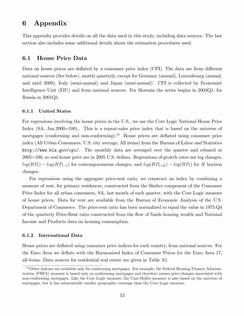
6 Appendix

This appendix provides details on all the data used in this study, including data sources. The last

section also includes some additional details about the estimation procedures used.

6.1 House Price Data

Data on house prices are deflated by a consumer price index (CPI). The data are from different

national sources (See below), mostly quarterly, except for Germany (annual), Luxembourg (annual,

and until 2009), Italy (semi-annual) and Japan (semi-annual). CPI is collected by Economist

Intelligence Unit (EIU) and from national sources. For Slovenia the series begins in 2003Q1; for

Russia in 2001Q1.

6.1.1 United States

For regressions involving the house prices in the U.S., we use the Core Logic National House Price

Index (SA, Jan.2000=100).. This is a repeat-sales price index that is based on the universe of

mortgages (conforming and non-conforming).18 House prices are deflated using consumer price

index (All Urban Consumers, U.S. city average, All items) from the Bureau of Labor and Statistics

http://www.bls.gov/cpi/. The monthly data are averaged over the quarter and rebased at

2005=100, so real house price are in 2005 U.S. dollars. Regressions of growth rates use log changes,

log(HPt) − log(HPt−1) for contemporaneous changes, and log(HPt+H) − log(HPt) for H horizon

changes.

For regressions using the aggregate price-rent ratio, we construct an index by combining a

measure of rent, for primary residences, constructed from the Shelter component of the Consumer

Price Index for all urban consumers, SA, last month of each quarter, with the Core Logic measure

of house prices. Data for rent are available from the Bureau of Economic Analysis of the U.S.

Department of Commerce. The price-rent ratio has been normalized to equal the value in 1975:Q4

of the quarterly Price-Rent ratio constructed from the flow of funds housing wealth and National

Income and Products data on housing consumption.

6.1.2 International Data

House prices are deflated using consumer price indices for each country, from national sources. For

the Euro Area we deflate with the Harmonized Index of Consumer Prices for the Euro Area 17,

all-items. Data sources for residential real estate are given in Table A1.

18Other indexes are available only for conforming mortgages. For example, the Federal Housing Finance Adminis-tration (FHFA) measure is based only on conforming mortgages and therefore misses price changes associated withnon-conforming mortgages. Like the Core Logic measure, the Case-Shiller measure is also based on the universe ofmortgages, but it has substantially smaller geographic coverage than the Core Logic measure.

53

\

Table A.1: Data sources for house prices.Australia Australian Bureau of Statistics. Exist. dwellings(8 CITIES),PER DWEL.,Q-ALL NSA. (1)Austria Oesterreichische National Bank. All dwellings(VIENNA),PER SQ.M.,Q-ALL NSA. (1)Belgium EXISTING DWELLINGS, PER DWEL.,Q-ALL NSA. (1)Canada Teranet- National Bank of Canada. Comp. 6 Cities (monthly, averaged to quarterly using sales pair count).Czech Republic Czech Statistical Offi ce. House prices.Denmark Statistics Denmark. ALL SINGLE-FAMILY HOUSE,PER DWEL,Q-ALL NSA.Estonia Statistical Offi ce of Estonia. Av. price per sq.m., 2-rooms and kitchen, Tallinn (1). 2009 onwards, 55-70m2.Euro Area European Central Bank. Euro area 17 (fixed composition); New and existing dwellings; Not S.A.Finland Statistics Finland. EXISTING HOUSES,PER SQ.M,Q-ALL NSA. (1)France National Institute of Statistics and Economic Studies. Existing Dwellings, Q-ALL NSA. (1)Germany Deutsche Bundesbank, based on data provided by BulwienGesa AG. Existing Dwellings, Y-ALL NSA. (1)Greece Bank of Greece. ALL DWELL.(URBAN GREECE EX.ATHENS),PER SQ.M, NSA. (1)Hungary FHB Bank. FHB House Price Index (actual buying and selling transaction data of residential real estate).Iceland Icelandic Property Registry. ALL DWELLINGS(GR. REYKJAVK),PER SQ.M,M-ALL NSA. (1)Ireland Economic and Social Research Institute (ESRI). ALL DWELLINGS, PER DWELLING., Q-ALL NSA. (1)Israel The Central Bureau of Statistics. Prices of Dwellings (Until September 2010 - Owner Occupied Dwellings).Italy Bank of Italy. ALL DWELLINGS, PER SQUARE M., H-ALL NSA. (1)Korea Kookmin Bank in Korea. ALL DWELLINGS, M-ALL NSA. (1)Luxembourg Central Bank of Luxembourg. ALL DWELLINGS, Y-ALL NSA. (1)Netherlands Statistics Netherlands. Existing own homes. Dwellings: all. Price index purchase prices.New Zealand The Reserve Bank of New Zealand. All dwellings, Q-ALL NSA. QVL. (1)Norway Statistics Norway. All dwellings, Q-AVG,NSA. (1)Poland Central Statistics Offi ce. Price of a square meter of usable floor space of a residential building.Portugal Inteligência de Imobiliário. All dwellings, PER SQUARE METER,M-ALL NSA. (1)Slovenia Statistical Offi ce of The Republic of Slovenia. Existing Dwellings,Q-ALL NSA. (1)Spain Bank of Spain. All dwellings, PER SQUARE M., Q-ALL NSA. (1)Sweden Statistics Sweden. ALL OWNER-OCCUPIED DWELLINGS,PER DWEL.,Q-ALL NSA. (1)Switzerland Swiss National Bank. ALL 1-FAMILY HOUSES,PER DWELLING,Q-ALL NSA.(1)United Kingdom Offi ce for National Statistics. All dwellings (ONS), PER DWEL.,M,Q-ALL NSA.(1)United States Federal Housing Finance Agency. Family Houses, Q-ALL NSA (all transactions, FHFA).(1)Russia Federal State Statistics Service. EXISTING DWELLINGS,PER SQUARE M,Q-ALL NSA.(1)China National Bureau of Statistics of China. Land prices, Resid. and Commercial, Q-ALL NSA. (1)

Notes: Series (1) can be found at the Bank of International Settlements website, http://www.bis.org/statistics/pp.htm.

6.2 Current Account Data

Current Account is measured as the current account deficit. Data are available from the Interna-

tional Monetary Fund for all countries except China. For China data are from State Administration

of Foreign Exchange, SAFE. CA balances are accumulated and deflated by 2006 GDP (collected by

Economist Intelligence Unit, EIU), in current US dollars. For Belgium, CA data 2000:Q1-2001:Q4

are from the National Bank of Belgium, provided by the Organization of Economic Cooperation

and Development (OECD).

United States: (CAdef/GDP )t is current account deficit over nominal GDP, at current market

prices. Balance of current account is from the Bureau of Economic Analysis, U.S. International

Transactions Accounts Data, in millions of dollars, not seasonally adjusted. GDP data is from the

Bureau of Economic Analysis, National Economic Accounts, in billions of current dollars, seasonally

adjusted at annual rates; we transform it to quarterly rates dividing by four.

International Data: (CAdef/GDP )t is current account deficit over nominal GDP, at current

market prices. Data from International Monetary Fund, in millions of US dollars, and GDP data

are collected by the Economist Intelligence Unit on nominal GDP (USD), quarterly.

54

6.3 Residential Investment

Residential Investment data are from Eurostat and national sources, as indicated in Table A.2.

Residential investment is accumulated and deflated by 2006 GDP, all in current national currency.

For France, Hungary, Poland, Switzerland and Russia, data is available only until 2009.

Table A.2: Data sources for residential investment.Australia Australian Bureau of Statistics. Private Gross fixed capital formation, Dwellings, Total , $ millionsAustria Eurostat.Belgium National Bank of Belgium. Gross fixed capital formation, dwellings, current prices, millions of Euros.Canada Statistics Canada, Capital formation in residential structures, current prices, national currency, NSA.Czech Republic Eurostat.Denmark Eurostat.Estonia Eurostat.Euro AreaFinland Eurostat.France Eurostat.Germany Eurostat.Greece Eurostat.Hungary Eurostat.Iceland Eurostat.Ireland Central Statistics Offi ce Ireland. Gross Dom. Physical Cap. Formation at current prices. Fixed capital, Dwellings.Israel Central Bureau of Statistics. Gross Domestic Capital Formation. Residential Buildings, current prices.Italy Eurostat.Japan Cabinet Offi ce, Gov. of Japan, Billions of Yen, nominal Private residential investment, not SA.Korea Bank of Korea, Gross fixed capital formation in residential buildings, current prices, Bil. Won.Luxembourg Eurostat.Netherlands Eurostat.New Zealand Statistics New Zealand. Gross Fixed Capital Formation, Residential buildings, current prices, $ Millions.Norway Norway Statistics. Gross fixed capital formation, Dwellings (households). Current prices (mill. NOK)Poland Eurostat.Portugal Eurostat.Slovenia Eurostat.Spain Eurostat.Sweden Eurostat.Switzerland Eurostat.United Kingdom Eurostat.United States US Bureau of Economic Analysis. Fixed Investment, Residential, Billions of dollars.Russia Federal State Statistics Service. Investment in fixed capital, in residential houses, current prices, billions rubles.China National Bureau of Statistics China (NBSC). Total Inv. Residential Buildings in the whole country, million yuan.

Notes: Most of the series are from national sources via Eurostat. Gross fixed capital formation, in construction work: housing,

millions of national currency, current prices.

6.4 Data on Credit Standards

6.4.1 United States

The variable CSt is a net percentage index that indicates the percentage of banks relaxing credit

standards for mortgage loans (both ’considerably’ and ’somewhat’), with respect to the previ-

ous quarter, minus the percentage of banks tightening credit standards (both ’considerably’ and

’somewhat’). This indicator is taken from the Senior Loan Offi cer Opinion Survey on Bank

55

Lending Practices for the US, published by The Federal Reserve. They report the net percent-

age of banks tightening standards. The negative of this is the net percentage of banks easing

standards, which we use in our empirical work. This is a quarterly survey of approximately

sixty large domestic banks and twenty-four U.S. branches and agencies of foreign banks. Ques-

tions cover changes in the standards and terms of the banks’ lending and the state of business

and household demand for loans. These data are available since May 1990, when the survey

then began including approximately 20 questions designed to measure changes in credit stan-

dards and terms on bank loans and perceived changes in the demand for bank credit. See

http://www.federalreserve.gov/boarddocs/snloansurvey/. We focus on the question that

asks about residential mortgage loans at each bank. From 1990Q2 (beginning of the Survey) to

2006Q4, the question is about residential mortgage loans in general:

Over the past three months, how have your bank’s credit standards for approving

applications from individuals for mortgage loans to purchase homes changed?

The recommendations for answering this question state

...If your bank’s credit standards have not changed over the relevant period, please

report them as unchanged even if the standards are either restrictive or accommodative

relative to longer-term norms. If your bank’s credit standards have tightened or eased

over the relevant period, please so report them regardless of how they stand relative to

longer-term norms. Also, please report changes in enforcement of existing standards as

changes in standards.

See http://www.federalreserve.gov/boarddocs/snloansurvey/ for more details.

From 2007Q1 onwards, the question is asked for each of three categories of residential mortgage

loans: prime residential mortgages, nontraditional residential mortgages, and subprime residential

mortgages. The answer to this question can be one of the following: tightened considerably, tight-

ened somewhat, remained basically unchanged, eased somewhat, eased considerably. Responses are

grouped in ’Large Banks’and ’Other Banks’. The index, however, is calculated using information

of “all respondents”. Given that the question is referenced to the past three months, we date the

index with respect to the quarter when changes to lending standards occurred (as opposed to when

the responses are collected, i.e., net percentage reported in July 2011 is the net percentage for

2011Q2). In the report beginning in 2007:Q1, a distinction is made between prime and subprime

mortgages in the survey. In the regressions using U.S. credit supply CS is a weighted average

of prime and subprime mortgages: (net percentage easing on prime)*weight plus (net percentage

easing on subprime)*(1-weight), where weight is 0.75 for 2007 and 0.95 for 2008. After that weight

equals 1, because no bank reported that they originated sub-prime mortgages. The earlier weights

56

are based on the paper http://www.jchs.harvard.edu/publications/finance/UBB10-1.pdf,

page 85, Figures 1-3. These numbers are approximately the average share of banks that originated

subprime residential mortgages, according to the Survey (23% for 2007 and 8% for 2008). Results

are not sensitive to using one or the other set of numbers.

We standardize the net percentage indicator by subtracting the mean and dividing by the

standard deviation.

6.4.2 International Data

CSt stands for credit standards for housing loans. Data are from bank lending surveys conducted by

national central banks, and the European Central Bank. The survey questions are modeled after the

U.S. Survey of Senior Loan Offi cers. Central Banks report the information in different ways. Some

Central Banks report net percentages, some report diffusion indices, and some report mean values.

Net percentage is the percentage of banks loosening (or tightening) credit standards with respect to

the previous quarter minus the percentage of banks tightening them (or relaxing). Diffusion index

is the percentage of banks loosening (or tightening) credit standards “considerably”with respect to

the previous quarter multiplied by 1 plus the percentage of banks loosening (or tightening) credit

standards “somewhat”multiplied by 0.5 minus the percentage of banks tightening (or relaxing)

“somewhat”times 0.5, minus the percentage of banks tightening (or relaxing) “considerably”times

1. Mean values: each answer receives a value from 1 to 5 (where for 5, the bank reported that relaxed

the credit standards “considerably”, 3 didn’t change them, and 1 is a “considerable”tightening),

and the mean value for each quarter is reported.

Mean values are a scale transformation of the diffusion index, but the net percentage indicator is

not. There are 9 countries for which we can construct either the diffusion index (Austria, Belgium,

Euro Area, France, Korea, Portugal, Spain, United States) or a mean value (Ireland) with the

information reported by the Central Banks. We have a larger set of 11 countries for which we have

only information on the net percentage (Canada and Netherlands). We standardize these indices,

country by country, by subtracting the mean and dividing by the standard deviation, for the period

2002Q4-2010Q4.

A positive value for CSt reflects easing credit conditions with respect to previous quarter, and

units are in terms of standard deviations.

Micro data for each country are not publicly available, but each of the countries above publishes

an indicator (net percentage, mean index, diffusion index) that reflects the change in credit condi-

tions in the country. The data sources are summarized in the table below. For Austria, Belgium,

Euro Area, France, Ireland, Netherlands, Portugal, Spain, the survey is based on the Bank Lending

Survey conducted by the European Central Bank (ECB).See http://www.ecb.int/stats/money/

surveys/lend/html/index.en.html. The European Central Bank’s website states:

57

The survey addresses issues such as credit standards for approving loans as well as

credit terms and conditions applied to enterprizes and households. It also asks for an

assessment of the conditions affecting credit demand. The survey is addressed to senior

loan offi cers of a representative sample of euro area banks and will be conducted four

times a year. The sample group participating in the survey comprises around 90 banks

from all euro area countries and takes into account the characteristics of their respective

national banking structures.

We focus on question 8 from the ECB survey, Item 8.1, Loans for house purchase:

Over the past three months, how have your bank’s credit standards as applied to the

approval of loans to households changed?

Respondents can reply one of the following answers: tighten considerably, tighten somewhat,

basically unchanged, ease somewhat, ease considerably.

For Korea and Canada, the raw questions in the survey differ somewhat. The survey for Korea

is from the Korean Survey of Lending Attitudes, which asks about households’“housing lending.”

The diffusion index is the sum of the responses of significant increase plus responses of moderate

increase minus responses of a significant decrease minus responses of moderate decrease times

0.5, divided by 100. For Canada, the Balance of Opinion survey delivers only a net percentage

indicator based only on overall lending conditions (inclusive of residential mortgages but also of

other forms of credit). The net percentage indicator we use is minus a weighted percentage of

surveyed financial institutions reporting tightened credit conditions plus the weighted percentage

reporting eased credit conditions.

Finally, when we analyze the intenational data in panel regressions, for the United States, we

construct a diffusion index (rather than use the net percentag indicator) from the data reported by

the Senior Loan Offi cer Opinion Survey on Bank Lending Practices for the US, published by The

Federal Reserve. Data for 2007 onwards is weighted average of prime and sub-prime mortgages,

with the following weights for prime mortgages: 2007, 0.75; 2008, 0.95; 2009 and 2010, 0. See

above.

Data sources for each country are given in Table A.3.

Table A.3: Data sources for credit standardsAustria Oesterreichische Nationalbank. Bank Lending Survey.Belgium Nationale Bank van Belgie. Bank Lending Survey.Canada Bank of Canada. Senior Loan Offi cer Survey. Lending conditions: Balance of Opinion.Euro Area European Central Bank. Bank Lending Survey.France Banque de France. Bank Lending Survey.Ireland Central Bank of Ireland. Bank Lending Survey. Mean.Korea Bank of Korea, Financial System Review. Survey Bank Lending Practices. Lending attitude.Netherlands De Nederlandsche Bank. Bank Lending Survey.Portugal Banco de Portugal. Bank Lending Survey.Spain Banco de Espana. Bank Lending Survey.United States Federal Reserve. Senior Loan Offi cer Opinion Survey.

58

Notes: For countries other than Korea and Canada, surveys follow the BLS survey conducted by the European Central Bank. In

that survey, the questions attained for our purpose are Q8.1 and Q13.1, about mortgage credit We construct diffusion indeces based on

this question for use in the Panel regressions. For Korea, we use the Lending Attitude diffusion index for households’housing, and for

Canada we use the ’Overall Balance of Opinion’diffusion index.

6.5 Estimation Details

6.5.1 U.S. Regressions

For the contemporaneous quarterly regressions we report Newey-West corrected standard errors

(and t-statistics) using 4 lags. For the long horizon quarterly regressions we use lags equal to

max{Horizon− 1, 4}, to take into consideration the use of overlapping data.

6.5.2 Panel Regressions

We use a balanced panel from 2002Q4 to 2010Q4, for 10 countries plus the Euro-Area: Austria,

Belgium, Canada, Euro Area, France, Ireland, Korea, Netherlands, Portugal, Spain, United States.

The choice of sample period is determined by the availability of a balanced panel for data on credit

standards (European Central Bank conducts the Bank Lending Survey since 2002Q4), and quarterly

house prices (For Italy and Germany we only have annual data on house prices, for Hungary only

semi-annual data on credit conditions, and for Poland we only have data on credit conditions

since 2003Q4). We also use a subsample of 9 countries where we drop Canada and Netherlands

(see information on credit standards, above). The Euro Area consists of 17 countries: Austria,

Belgium, Cyprus, Estonia, Finland, France, Germany, Greece, Ireland, Italy, Luxembourg, Malta,

the Netherlands, Portugal, Slovakia, Slovenia, and Spain. We construct log changes, log(HPt) −log(HPt−1) for contemporaneous changes, and log(HPt+H)− log(HPt) for H horizon changes.

For the contemporaneous quarterly regressions, we report the robust standard errors (and t-

statistics) using the Driscoll-Kraay statistic, with lags=3 (default). For the quarterly long horizon

regressions, we use instead number of lags equal to max{Horizon− 1, 3} to take into account theuse of overlapping data. For more on Driscoll-Kraay statistic, see Robust Standard Errors for Panel

Regressions with Cross-Sectional Dependence, by Daniel Hoechle,

http://fmwww.bc.edu/repec/bocode/x/xtscc\_paper.pdf. and Driscoll and Kraay (1998).

59

References

Acharya, V. V., M. Richardson, S. Van Nieuwerburgh, and L. J. White (2011): Guar-

anteed To Fail: Freddie, Fannie, and the Debacle of U.S. Mortgage Finance. Princeton University

Press.

Acharya, V. V., P. Schnabl, and G. Suarez (2010): “Securitization Without Risk Transfer,”

NBER Working Paper No. w15730.

Adam, K., A. Marcet, and P. Kuang (2011): “House Price Booms and the Current Account,”

Working Paper.

Adelino, M., A. Schoar, and F. Severino (2011): “Credit Supply and House Prices: Evidence

from Mortgage Market Segmentation,”Working Paper.

Aizenman, J., and Y. Jinjarak (2009): “Current account patterns and national real estate

markets,”Journal of Urban Economics, 66(2), 75—89.

Amromin, G., J. Huang, C. Sialm, and E. Zhong (2011): “Complex Mortgages,” WP

NBER17315.

Barlevy, G., and J. D. Fisher (2011): “Mortgage Choices and Housing Speculation,”Federal

Reserve Bank of Chicago, WP2010-12.

Bernanke, B. S. (2005): Remarks by Governor Ben S. Bernanke at the Sandridge Lecture,

Virginia Association of Economics, Richmond, Virginia, March 10, 2005.

(2008): Remarks by Chairman Ben S. Bernanke at the International Monetary Conference,

Barcelona, Spain (via satellite), June 3, 2008.

(2011): “International Capital Flows and the Returns to Safe Assets in the United States

2003-2007,”Banque de France Financial Stability Review, 15, 13—26.

Bernanke, B. S., and M. Gertler (1989): “Agency Costs, Net Worth and Business Cycle

Flutuations,”American Economic Review, 79, 14—31.

Bernanke, B. S., V. R. Reinhart, and B. P. Sack (2004): “Monetary Policy Alternatives

at the Zero Bound: An Empirical Assessment,”Brookings Papers on Economic Activity, (2),

1—100.

Boz, E., and E. Mendoza (2011): “Financial Innovation, the Discovery of Risk, and the U.S.

Credit Crisis,”Unpublished paper.

60

Caballero, R. J., E. Fahri, and P.-O. Gourinchas (2008): “An Equilibrium Model of

“Global Imbalances”and Low Interest Rates,”American Economic Review, 98(1), 358—393.

Caballero, R. J., and A. Krishnamurthy (2009): “Global Imbalances and Financial

Fragility,”American Economic Review Papers and Proceedings, 99, 584—588.

Case, K. E., and R. J. Shiller (1989): “The Effi ciency of the Market for Single-Family Homes,”

American Economic Review, 79(1), 125—137.

Driscoll, J. C., and A. C. Kraay (1998): “Consistent Covariance Matrix Estimation With

Spatially Dependent Panel Data,”The Review of Economics and Statistics, 80(4), 549—560.

Favara, G., and J. Imbs (2011): “Credit Supply and the Price of Housing,”Working Paper.

Favilukis, J., S. C. Ludvigson, and S. Van Nieuwerburgh (2009): “The Macroeconomic

Effects of Housing Wealth, Housing Finance and Limited Risk Sharing in General Equilibrium,”

Unpublished paper, New York University.

(2011): “Foreign Ownership of U.S. Safe Assets: Good or Bad?,” Unpublished paper,

New York University.

Ferrero, A. (2011): “House Prices Booms and Current Account Deficits,”Unpublished paper,

Federal Reserve Bank of New York.

Geithner, T. (2007): Remarks by New York Federal Reserve President Timothy Geithner at

the Council on Foreign Relations’C. Peter McColough Roundtable Series on International Eco-

nomics, New York City, January 11, 2007.

Gete, P. (2010): “Housing Markets and Current Account Dynamics,”Unpublished paper.

Glaeser, E. L., J. D. Gottlieb, and J. Gyourko (2010): “Can Cheap Credit Explain The

Housing Boom?,”Unpublished Paper, Harvard University.

Haughwout, A., J. Tracy, R. Peach, and E. Okah (2011): “Mortgages Defaults and the

Credit Crunch,”Unpublished.

Himmelberg, C., C. Mayer, and T. Sinai (2005): “Assessing High House Prices: Bubbles,

Fundamentals and Misperceptions,”Journal of Economic Perspectives, 19(4), 67—92.

Hodrick, R., and E. C. Prescott (1997): “Post-War U.S. Business Cycles: A Descriptive

Empirical Investigation,”Journal of Money, Credit, and Banking, 29, 1—16.

Keys, B. J., T. Piskorski, A. Seru, and V. Vig (2011): “Mortgage Financing in the Housing

Boom and Bust,”Unpublished paper.

61

Kiyotaki, N., and J. Moore (1997): “Credit Cycles,”Journal of Political Economy, 105(2).

Kohn, D. L. (2002): “Panel: Implications of Declining Treasury Debt. What Should the Federal

Reserve Do as Treasury Debt Is Repaid?,”Journal of Money, Credit and Banking, 34(3), 941—

945.

Kole, L. S., and R. F. Martin (2009): “The Relationship Between House Prices and the Current

Account,”Board of Governors of the Federal Reserve System, Working Paper.

Krainer, J., S. F. LeRoy, and O. Munpyung (2009): “Mortgage default and mortgage valu-

ation,”Working Paper Series 2009-20, Federal Reserve Bank of San Francisco.

Krishnamurthy, A., and A. Vissing-Jorgensen (2010): “The Aggregate Demand for Trea-

sury Debt,”Unpublished paper, Kellog School, Northwestern University.

Laibson, D., and J. Mollerstrom (2010): “Capital Flows, Consumption Booms and Asset

Bubbles: A Behavioural Alternative to the Savings Glut Hypothesis,”Economic Journal, 120,

354—374.

Laufer, S. (2011): “Equity Extraction and Mortgage Default,”Working Paper. New York Uni-

versity.

Lee, D., C. Mayer, and J. Tracy (2011): “A New Look at Second Liens,”Working Paper.

Maddaloni, A., and J.-L. Peydro (2011): “Bank Risk-taking, Securitization, Supervision, and

Low Interest Rates: Evidence from the Euro-area and the U.S. Lending Standards,”The Review

of Financial Studies, 24(6).

Mendoza, E. G., V. Quadrini, and J.-V. Rios-Rull (2007): “Financial Integration, Financial

Deepness and Global Imbalances,”NBER Working Paper No. 12909.

Mian, A., and A. Sufi (2009): “The Consequences of Mortgage Expansion: Evidence from the

U.S. Mortgage Default Crisis,”Quarterly Journal of Economics, 124(4), 1449—1496.

Mian, A., A. Sufi, and F. Trebbi (2009): “The Political Economy of the U.S.

Mortgage Default Crisis,” Chicago GSB Research Paper No. 08-17. Available at SSRN:

http//ssrn.com/abstract=1291524.

Newey, W. K., and K. D. West (1987): “A Simple, Positive Semidefinite, Heteroskedasticity

and Autocorrelation Consistent Covariance Matrix,”Econometrica, 55, 703—708.

Nichols, J., A. Pennington-Cross, and A. Yezer (2005): “Borrower Self-Selection, Un-

derwriting Costs, and Subprime Mortgage Credit Supply,”Journal of Real Estate Finance and

Economics, 30, 197—219.

62

Obstfeld, M. (2011): “Financial Flows, Financial Crises, and Global Imbalances,” Keynote

address to the 15th International Conference on Macroeconomic Analysis and International

Finance, 26-28 May, 2011, University of Crete, Greece.

Rajan, R., and R. Ramcharan (2011a): “The Anatomy of a Credit Crisis: The Boom and Bust

in Farm Land Prices in the United States in the 1920s,”Working Paper.

(2011b): “Constituencies and Legislation: The Fight over the McFadden Act of 1927,”

Working Paper.

Rice, T., and P. E. Strahan (2010): “Does Credit Competition Affect Small-Firm Finance?,”

The Journal of Finance, 65(3), 861—889.

Streitfeld, D. (2009): “Tight Mortgage Rules Exclude Even Good Risks,”The New York Times,

Saturday, July 11, p. A1.

Taylor, J. B. (2009): Getting Off Track: How Government Actions and Interventions Caused,

Prolonged, and Worsened the Financial Crisis. Hoover Institution Press, Stanford.

U.S. Treasury Department (2011): “Report on Foreign portfolio Holdings of U.S. Securities,

as of June 30, 2010,” Department of Treasury, Federal Reserve Bank of New York, Board of

Governors of the Federal Reserve System.

Warnock, F. (2010): “Two Myths About the U.S. Dollar,”Capital Flows Quarterly.

Warnock, F. E., and V. C. Warnock (2009): “International Capital Flows and U.S. Interest

Rates,”Journal of International Money and Finance, 28, 903—919.

63