industrial structure and capital flows

American Economic Review 2012, 102(5): 2111–2146 http://dx.doi.org/10.1257/aer.102.5.2111

2111

Industrial Structure and Capital Flows†

By Keyu Jin*

This paper provides a new theory of international capital flows. In a framework that integrates factor-proportions-based trade and finan-cial capital flows, a novel force emerges: capital tends to flow toward countries that become more specialized in capital-intensive indus-tries. This “composition” effect competes with the standard force that channels capital toward the location where it is scarcer. If the compo-sition effect dominates, capital flows away from the country hit by a positive labor force/productivity shock—a flow “reversal.’’ Extended to a quantitative framework, the model generates sizable current account imbalances between developing and developed countries broadly consistent with the data. (JEL F14, F21, F32, F41, L16, O19)

Commodity trade and capital flows are the two engines of globalization. Until now, little has been known about how they interact. The conventional analyses of international macroeconomics and trade theory in separation fails to account for the influence of macroeconomic dynamics on the structure of trade as well as the aggre-gate feedback effects of trade patterns. This paper demonstrates that their interaction can be crucial in determining the global allocation of capital, shedding new light on widely-debated issues surrounding global imbalances.

The main purpose of this paper is to develop a general-equilibrium framework that integrates a factor-proportions paradigm of trade and financial capital flows, allow-ing for their interplay. From only basic ingredients, it derives new results on how the global equilibrium responds to a variety of shocks and structural changes. In con-trast to predictions from the standard open-economy macroeconomic framework, a permanent increase in the labor-force or labor productivity in a country can induce a net capital outflow. Also, capital can flow from developing countries to advanced economies when these countries integrate. The underlying mechanism hinges on a new force driving international capital flows: capital tends to flow toward econo-mies that become more specialized in capital–intensive sectors—a “composition” effect. Simultaneously present is the standard, “convergence” effect, which channels capital toward where the effective capital-labor ratio is lower. These two forces can

* Department of Economics, London School of Economics and Political Science, Houghton Street WC2A 2AE (e-mail: [email protected]). This paper is part of my doctoral thesis at Harvard University, under the supervision of Kenneth Rogoff, whom I would like to thank for his continual guidance and support. My deep gratitude extends to Robert Barro, Emmanuel Farhi, and Gita Gopinath for their invaluable advice. Professors Pol Antrás, John Campbell, Richard Cooper, Arnaud Costinot, Alejandro Cuñat, Elhanan Helpman, Marc Melitz, Nathan Nunn, and Harvard International Economics Workshop and Macroeconomics workshop participants offered helpful comments. I also thank Gianluca Benigno, Stéphane Guibaud, Kai Guo, Ethan Ilzetzki, Oleg Itskhoki, Karthik Kalyanaraman, Jean Lee, Robert McMillan, Paolo Pesenti, Hélène Rey, Dan Sacks, Florent Ségonne, Jaume Ventura, and Alwyn Young. Attakrit Leckcivilize provided excellent research assistance. I would also like to thank three anonymous referees.

† To view additional materials, visit the article page at http://dx.doi.org/10.1257/aer.102.5.2111.

Contents

Industrial Structure and Capital Flows† 2111

I. The Model Description 2114

A. Production Technologies 2115

B. Consumers 2117

C. Market Clearing 2118

D. Equilibrium 2119

II. The Composition Effect 2122

A. Aggregate Savings and Investment 2124

B. International Capital Flows 2127

III. Quantitative Analysis 2128

A. A Multi-Period OLG Model 2128

B. Calibration 2129

C. Results 2131

D. Discussion 2134

IV. Suggestive Empirical Evidence 2135

V. Final Remarks 2139

Appendix 2140

I. Derivations of the Analytical Model 2140A. The Two-Country, Two-Period Multi-Sector OLG Model 2140B. Special Case: A Closed-Form Solution 2142C. Initial Equilibrium 2143II. Computational Algorithm 2143III. Data Appendix 2143

REFERENCES 2144

http://dx.doi.org/10.1257/aer.102.5.2111

mailto:[email protected]


2112 THE AMERICAN ECONOMIC REVIEW AuGuST 2012

become competing, and the direction of capital flows depends on which one of the two effects dominates.

Two of the most important phenomena in the global economy have been trade and financial integration and rapid labor force/productivity growth in emerging mar-kets. The standard open-economy models predict a net capital inflow into develop-ing countries—the opposite of what is actually happening. Yet, the basic underlying assumption in these workhorse frameworks is that countries cannot engage in intra-temporal commodity trade but only in intertemporal trade. This assumption becomes untenable when these large-scale forces alter a country’s comparative advantage, and consequently, its structure of trade.1

How can changes in the structure of trade and specialization patterns affect capital flows? The starkest example illustrating the relationship between a country’s com-position of production and its demand and supply of capital is the case of complete specialization. Assume that one country, “Home,” fully specializes in producing a capital-intensive good that uses capital and labor as an input to production, and the other country, “Foreign,” fully specializes in producing a labor-intensive good that uses only labor as an input. Foreign generates labor income, but in the absence of domestic demand for capital, it always saves in Home. A labor force/productivity boom in Foreign can only lead to a capital outflow. This limiting case is obviously extreme but the intuition carries over to the more general case where all sectors use both factors of production and countries produce all goods (incomplete and endog-enous specialization). The demand for capital in a country relative to its supply of savings hinges on its industrial structure. An industrial structure that is tilted toward capital-intensive sectors will face greater investment demands, and thus a high share of output accruing to investment, at the same time generating a low share of output accruing to labor income. An industrial structure that concentrates on producing labor-intensive goods will see exactly the opposite. Thus in a fully-integrated world economy, a country that experiences a labor force/productivity shock (Foreign) that causes its production structure to shift toward labor-intensive goods will tend to see a net capital outflow.

The analytical framework developed in this paper is a stochastic two-country overlapping generations model with production and capital accumulation, based on the closed-economy, one-good framework in Abel (2003).2 Multiple tradable sectors that differ in factor intensity are incorporated to capture factor-proportions-based trade, and financial capital is allowed to flow across borders.3 Adjustment costs serve to pin down the country-level capital stock in a world of factor price

1 Romalis (2004) finds that countries tend to capture larger shares of world production and trade for commodities that require more intensive use of their abundant factors, and that countries that rapidly accumulate a factor see their production and export structures systematically shift toward industries that intensively use that factor.

2 Abel (2003) develops a closed-economy, one-sector overlapping-generations model with capital adjustment costs to analyze the effect of a baby boom on stock prices and capital accumulation.

3 The key difference between this framework and the Heckscher-Ohlin-Mundell framework is the incorporation of a realistic macroeconomic environment. The first distinguishing feature is that capital stock takes one period to adjust—as is standard in macroeconomic models. Specifically, capital stock in each sector is augmented by investment rather than through the reallocation of capital across sectors. This feature is reminiscent of the “specific-factors model” in the trade literature (Jones 1971; Amano 1977; Neary 1978; Brecher and Findlay 1983). Second, the notion of capital mobility is no longer restricted to the static allocation of capital across countries for a fixed level of world capital stock, but pertains to one in which capital flows are driven by the allocation of savings across countries. Third, there is simultaneous mobility in trade flows and capital flows.

2113JIN: INDuSTRIAL STRuCTuRE AND CAPITAL FLOWSVOL. 102 NO. 5

equalization.4 One advantage of this framework is its analytical tractability. Closed-form solutions can be obtained in a special case of this open-economy stochastic growth model with multiple tradable sectors, making transparent the key mecha-nisms that underpin the new results.

I show that in this integrated framework it is possible to isolate the convergence effect and the composition effect in order to examine their disparate impact on capital flows. The standard, familiar neoclassical case becomes one of two special cases in an integrated framework—namely, the case when sectors feature no differences in factor intensities, and only the convergence effect is present. The other special case, in which the most labor-intensive sector uses only labor as an input to production, isolates the composition effect. In the general case, the convergence effect and the composition effect coexist and the condition under which the latter effect dominates is that factor intensities be sufficiently different so that specialization patterns are pronounced.

The standard open-economy models are the one-good or two-good stochastic growth models of large open economies (Backus, Kehoe, and Kydland 1992, 1994). These models allow for capital flows across borders but factor-proportions trade is absent. The overlapping generations structure featured in the model is analytically convenient although not essential.5 Two-sector, two-country models which feature factor-proportions trade, on the other hand, usually assume that capital cannot flow across countries. Examples include Beaudry and Collard (2006); Ventura (1997); Atkeson and Kehoe (2000); Mundell (1957), among others. The purpose of examin-ing the interaction between trade and capital flows calls for both trade and financial mobility, a feature which distinguishes this paper from the works in these two sets of literature. Cuñat and Maffezzoli (2004) is an example that allows for both trade and financial mobility, although it focuses on the business cycle properties of a two-country model with Hecksher-Ohlin trade, paying particular attention to the correla-tion between the terms of trade and output.

Recent interest has emerged in examining the relationship between commodity trade and capital flows. Ju and Wei (2007, 2009) incorporate labor market rigidity in a dynamic Heckscher-Ohlin framework. Ju and Wei (2007) examine how labor market rigidity affects the size of current account adjustment to shocks and its adjustment speed to the long run equilibrium.6 Ju and Wei (2009) show that in the same frame-work, capital can flow from a labor-abundant country to a capital-abundant country when there is a positive productivity increase in the labor-intensive sector of the for-mer. Antras and Caballero (2009) examine the relationship between trade and capital

4 With factor price equalization, capital earns the same returns everywhere and can be located anywhere. A com-mon way of pinning down capital stock is to assume balanced trade—that capital cannot flow across borders. See Beaudry and Collard (2006) and Atkeson and Kehoe (2000) as recent examples. However, adjustment costs can be shut off and FPE will not occur as a result of risk in a stochastic, incomplete-markets model. Further discussions can be found in footnote 18.

5 A technical Appendix showing similar results in a representative-agent model is available upon request.6 They show that the degree of labor market frictions in a country affects the size and speed of current account

adjustment to shocks, in a small open economy. When there is some degree of mobility in both trade and capital, an economy’s adjustment to shocks involves a combination of a change in the composition of goods trade (intra-temporal trade) and the current account (intertemporal trade). In the extreme case that labor is sector specific, all adjustment to shocks takes place through intertemporal trade. Thus, relatively more rigid labor regulations induce a larger response in the current account, and slow down the speed of adjustment of the current account toward the long-run equilibrium.


flows when countries differ in financial development and sectors differ in financial dependence. They find that trade and capital flows can become complements.7

What sets this paper apart from these other works is its focus on isolating trade and specialization—arising from changes in endowment and productivity alone— as drivers of capital flows. In contrast, market frictions play a key role in deter-mining the structure of trade and specialization patterns in these other works, and hence alter the relationship between trade and capital flows. Ju and Wei (2007, 2009) exhibit some conceptual similarities with the current work in that it also fea-tures multiple sectors with different factor intensities. However, the main mecha-nism driving the results in the present paper—the “composition effect’’— does not arise in their model for the reason that in addition to labor market rigidity—which obstructs labor reallocation—trade costs, and costs to international capital flows in their framework all work against comparative advantage in its impact on shaping specialization patterns.8

Finally, in terms of explaining global imbalances—in particular the net flow of capital from certain developing countries to industrialized countries—this paper proposes an alternative view highlighting the importance of trade and specialization, in contrast to works that put financial heterogeneity at center stage, including Ju and Wei (2006); Caballero, Farhi, and Gourinchas (2008); and Mendoza, Quadrini, and Rios-Rull (2009). Gourinchas and Jeanne (2009) focus on the allocation of capital across developing countries and show that in the data, capital tends to flow more to countries that invest and grow less, the opposite of the prediction of the neoclassical growth model. Aguiar and Amador (2010) provide a political economy perspective, with contracting frictions, on why countries which grow fast tend to experience net capital outflows.

The rest of the paper is organized as follows. The multiple-sector framework is described in Section I. A special case that isolates the composition effect and emits a closed-form solution characterizing the evolution of capital and international capital flows is presented in Section II. The quantitative predictions of the general model is presented in Section III, and Section IV explores its empirical implications. Finally, Section V concludes.

I. The Model Description

Consider a world with two countries, Home (h) and Foreign ( f ), each charac-terized by an overlapping generations economy in which consumers live for two periods. A consumer supplies one unit of labor when young and does not work when old. The assumption of a two-period model is important only for analytical

7 The financial friction in their paper limits the amount of capital allocated to the financially-constrained sector, and the degree of financial contractibility can vary across countries. By allowing the South to specialize in a sector with lower financial frictions, international trade reduces the negative impact of financial underdevelopment on the rental rate of capital, and causes the return to capital to be higher in the South. The implication is thus that, in the presence of asymmetric financial development, trade integration increases capital flows from the North to the South.

8 In addition, capital can adjust costlessly across sectors within a country, as in the Heckscher-Ohlin model. The ability to instantaneously adjust capital across sectors, within a country, while international capital flows are costly, substantially dampens the need for cross-border flows. Another important difference is that in this paper, the reversal of capital flows can also occur in ex ante symmetric countries, whereas in their paper it only occurs when the labor-abundant country experiences a productivity increase in its labor-intensive sector.


convenience, and is relaxed in the quantitative analyses undertaken in Section III. Each country uses identical technology to produce intermediate goods i = 1, … , m, which are traded freely and costlessly. Intermediate goods are combined to pro-duce a composite good that is used for consumption and investment. Preferences and production technologies are assumed to have the same structure and parameter values across countries. However, the technologies differ in two aspects: in each country, the labor input consists only of domestic labor, and intermediate-goods-producing firms are subject to country-specific productivity and labor force shocks. Henceforth, j denotes countries and i denotes sectors.

A. Production Technologies

The production technology, identical in each country, uses capital and labor to produce an intermediate good. Let Y it j

be the gross production of intermediate good i in country j :

(1) Y it j = ( K it j

) α i ( A t j N it j ) 1− α i ,

where 0 < α i < 1 for all i, and α i ’s are indexed in such a way that α 1 < α 2 ⋯ < α i ⋯ < α m . Let K it j

be j ’s aggregate capital stock in sector i at the beginning of period t, and N it j

be the aggregate input of labor employed in sector i. The country-specific labor productivity A t j evolves according to

ln A t j = ln A t−1

j + ϵ At

j ,

where the growth rate of labor productivity, ϵ At j , is an i.i.d. random variable. A high

realization of ϵ At j represents a productivity boom in country j.

The intermediate goods produced by the production technology are combined to form a unit of a composite good, used for both consumption and investment. Let

I it j = [ ∑

k=1

m

γ k 1 _ θ ( x ki, t j

) θ−1 _ θ ]

θ _ θ−1

,

where x ki, t j denotes the amount of good k used for investment in the i th sector of

country j, ∑ i=1 m γ i = 1, and θ > 0.

In the absence of barriers to international trade, the law of one price holds for all intermediate goods, and there is one international price associated with each good i, denoted p it . That preferences are symmetric across countries implies that the associ-ated investment price index in any country is the same, and is given by

(2) P t = [ ∑ i=1

m

γ i p it 1−θ ]

1 _ 1−θ

,

which for simplicity is normalized to 1.


The capital used in producing good i in country j is augmented by investment goods, I it j

and the current capital stock K it j . The law of motion for capital stock

is given by K i, t+1 j = G( K it j

, I it j ) where G( K it j

, I it j ) is nondecreasing and linearly

homogeneous in K it j and I it j

. Convex adjustment costs are represented by therestriction ∂ 2 G j

_ ∂ I it j 2

< 0. Following Abel (2003), I take a log-linear specification of G( K it j

, I it j ),

(3) K i, t+1 j = a( I it j

) ϕ ( K it j ) 1−ϕ ,

where 0 < ϕ < 1 and a > 0. As in Abel (2003), this log-linear capital accumula-tion equation reduces to the one in the neoclassical growth model with complete depreciation in each period if ϕ = 1 and a = 1. On the other hand, if ϕ = 0 and a = 1, it is reduced to the case of the Lucas-tree asset pricing model in which the capital stock is constant. Compared to the standard capital accumulation equation with adjustment costs,

(4) K i, t+1 j = (1 − δ) K it j

+ I it j − b _

2 ( I it j

_ K it j − δ )

2

K it j ,

the log-linear model and the standard model are equivalent up to the second order if a = ϕ −ϕ , δ = ϕ, and b = 1 − ϕ

_ ϕ , where δ is the depreciation rate. The purpose of adopting the log-linear specification is to derive an analytical solution for the equilibrium quantity of capital, presented in Section II. The subsequent quantitative analyses in Section III adopt the standard capital accumulation equation (4).

Let q it j be the price of capital in sector i and country j at t. It is the price, in terms

of the composite good, of acquiring one unit of capital at the end of period t to be carried into period t + 1. Thus, the price is the additional I it j

needed to augment K i, t+1 j

by one unit, that is, (∂ K i, t+1 j /∂ I it j

) −1 . For ϕ > 0, equation (3) implies that

(5) q it j = 1 _

aϕ ( I it j _ K it j )

1−ϕ

.

If 0 < ϕ < 1, then q it j is increasing in sector i’s investment-capital ratio, I it j

/ K it j . The

value, in terms of the composite good, of the aggregate capital stock in sector i to be carried into period t + 1 is q it j

K i, t+1 j , which, by equations (3) and (5), implies that

(6) q it j K i, t+1 j

= I it j _ ϕ .

Factor markets are competitive so that each factor, capital and labor, earns its mar-ginal product. The wage rate per unit of labor in sector i in country j is

(7) w it j = (1 − α i ) p it

Y it j _

N it j .


Since labor is perfectly mobile across sectors within any country j, the wage rate in each sector i in any period t, w it j

, is equal to the country-specific wage rate w t j .Following Abel (2003), the total rental to capital in any period can be interpreted

as the sum of the rentals of capital earned in the intermediate-production process, and in the capital adjustment process, where capital also contributes to lower instal-lation costs next period. The rental earned in period t by the capital stock in sector i

and country j is α i p it Y it j

_ K it j

. The rental earned in the capital adjustment process at

time t is the marginal contribution of capital in augmenting capital stock for use in

the following period, d K t+1 j

_ d K t j

, multiplied by the relative price of capital q it . It follows

from equations (3) and (5) that this rental is equal to 1 − ϕ _ ϕ I t

j _

K t j . The rate of return to

capital of sector i in country j during period t is thus the sum of these two rent-als, divided by the price at which it was purchased in the previous period, q i, t−1 j

, which gives9

(8) R it j =

α i p it Y it j

_

K it j + 1 − ϕ _ ϕ I it

j _

K it j __ q i, t−1 .

B. Consumers

At the beginning of period t, a measure N t j of consumers are born in country j, where N t j evolves according to

ln N t j = ln N t−1 j + ϵ N, t j

,

with ϵ N, t j being an i.i.d. random variable that is independent of ϵ A, t j

at all leads and lags. A high realization of ϵ N, t j

represents a labor force boom in country j. In period t, a young consumer in Home inelastically supplies one unit of labor and

earns the competitive wage w t h , which is used for consumption c t y, h , and for purchas-ing capital. Let k i, t+1 h, j

be the amount of capital that a young consumer in Home buys in sector i from country j, at a price q it j

per unit, at the end of period t to be carried into period t + 1. In Home, a young consumer’s consumption and purchases of capital satisfy

(9) c t y, h = w t h − ∑ j=h, f

∑ i=1

m

q it j k i, t+1 h, j

.

9 When combined with the consumer’s problem in Section IB, the rate of return to capital can also be understood from the point of view of an old consumer who purchased the capital stock in the previous period and is going to sell it to the young consumers in the current period. The rate of return to capital is thus the sum of the dividend income p it Y it j

− w it j N it j

− I it j and the market value of capital stock from selling it to the younger consumers in period t,

q it j K i, t+1 j

, divided by the market value of capital stock when purchased in the previous period, q i, t−1 j K it j

.


Assume that consumers do not have bequest motives, and therefore consume all available resources when they are old. The consumption of an old Home consumer in period t + 1, denoted as c t+1 o, h

, is entirely financed by capital, so that

(10) c t+1 o, h = ∑

j=h, f

∑ i=1

m

R i, t+1 j q it j

k i, t+1 h, j .

The lifetime utility of consumption that a Home consumer born in the beginning of period t maximizes is

(11) u t = ( c t y, h ) 1−ρ _

1 − ρ + β 피 t [ ( c t+1 o, h ) 1−ρ _ 1 − ρ ],

where β denotes the discount factor, and satisfies 0 < β < 1, c t y, j denotes the con-sumption of a young consumer in j in period t, and c t+1 o, j

denotes the consumption of an old consumer in j in period t + 1. The aggregate consumption index in j at t is

(12) C t j = [ ∑ i=1

m

γ i 1 _ θ ( c it j

) θ−1 _ θ

] θ _ θ−1

,

where c it j is the consumption demand for good i in j. Since the composite good used

for consumption is the same composite good used for investment, the consumer price index is given by equation (2).

C. Market Clearing

The intermediate goods markets clear when global demand of any good i equals its global supply. Let Y it g

denote the global output of good i, where Y it g

≡ ∑ j=h, f Y it j

(henceforward, g denotes global variables). Market clearing for each good i requires that

(13) Y it g = ∑

j=h, f

c it j + ∑

j=h, f

∑ k=1

m

x ki, t j ,

where

c it j = γ i ( p it ) −θ C t j

and

x ki, t j = γ i ( p it ) −θ I it j

.

If θ = 1, consumers devote a constant share γ i of total spending to good i. Let I t j = ∑ i=1

m I it j

denote country j ’s aggregate investment in period t. Replacing these


expressions for c it j and x ki j

into equation (13) yields the relative price of any two intermediate goods i and k:

(14) p it _ p kt

= ( γ i _ γ k Y kt

g _ Y it g )

1 _ θ

.

The relative price of any two goods falls with respect to an increase in the relative output of the two goods with an elasticity 1/θ. When θ = 1, relative output changes are completely offset by relative price changes so that the nominal values of output remain constant across sectors.10

Lastly, domestic labor markets clear when

∑ i=1

m

N it j = N t j

for any j. The world resource constraint says that the total amount of final goods in the world, denoted as Y t g , is used for two purposes: consumption and capital forma-tion. Let I t g = ∑ j

I t j denote world investment in period t. Then, the world resource

constraint requires that

(15) Y t g ≡ ∑ i=1

m

p it Y it g = C t g + I t g ,

where C t g = ∑ j ( N t j c t y, j + N t−1 j

c t o, j ). GDP at time t in any country j is defined to be the total value of consumption in j and the market value of capital stock in j, at time t:

GD P t j = ∑ i=1

m

p it Y it j + 1 − ϕ _ ϕ I t j ,

where the second equality comes from equation (6).11

D. Equilibrium

A semi-closed form solution of the equilibrium of the economy follows when relying on three simplifying assumptions, summarized below:

ASSUMPTION 1: unitary elasticity of substitution of intermediate goods (θ = 1).

ASSUMPTION 2: Consumers have logarithmic preferences ( ρ = 1).

ASSUMPTION 3: The capital-adjustment technology is log-linear, as in equation (3).

10 When θ = 1, the value of output in any industry i is a constant fraction γ i of the total value of world output, so that p it Y it g

= γ i ∑ k=1 m p kt Y kt g

.11 World GDP, GD P t g = ∑ j

G D P t j , exceeds Y t g by [(1 − ϕ)/ϕ] Y t g , which is the value added by the capital adjust-

ment technology.


Assumption 2 simplifies the consumption/saving problem and implies that private sav-ing does not depend on the real rate of return. Severing the link through which the rate of return affects capital accumulation allows for analytical expressions for the optimal level of consumption in each country. When Assumptions of 1 and 3 are combined with Assumption 2, the global aggregate investment-output ratio and the global industry-level investment-output ratio are both constants. Relying on these results, the evolution of the capital stock in each sector i in any country j, is characterized by one key vari-able—the present discounted value of the expected share of good i produced domesti-cally. Without these assumptions, neither the semi-closed form solution in the general case nor the full-closed form solution in the special case, presented in Section II, is possible. In later sections, all of these assumptions are relaxed, and it is shown that none is crucial for the main qualitative results of interest.

Assuming that consumers have logarithmic utility, the optimal consumption of a young consumer in period t is a constant fraction of the present value of lifetime resources, which, in this setting, is simply the wage income earned by the young. The optimal consumption of a young consumer in j is therefore

(16) c t y, j = 1 _ 1 + β w t j .

Let C t y, j be the aggregate consumption of the young cohort, where C t y, j = N t j c t y, j . Aggregating this across countries implies that the world consumption of the young in period t, C t y, g ≡ ∑ j

C t y, j , is a constant fraction of world labor income,

W t g ≡ ∑ j w t j N t j . With a unitary elasticity of substitution (Assumption 1), W t g is

a constant share s l = ∑ i γ i (1 − α i ) of world output, where s l can be interpreted as a

weighted-average labor share, the weights being the expenditure share of good i, γ i . It follows that the global investment-output ratio is a constant:12

(17) I t g _ Y t g

= ψ s l ,

where ψ = ϕβ _

1 + β . How is world investment allocated across industries and coun-tries? To determine global investment at the industry level, let I it

g = μ it I t g so that

μ it represents the share of industry i’s investment in aggregate investment, and let I it j

= η it j I it g

so that η it j represents j’s share of global investment in sector i. Investment

in any sector i, in any country j, can thus be written as

(18) I it j = μ it η it j

I t g ,

where

(19) ∑ j

η it j = 1, ∑

i=1

m

μ it = 1.

12 Aggregating equation (9) across countries gives C t y, g = W t g − ∑ j ∑ i

q it j

K i, t+1 j , where K i, t+1 j

= k i, t+1 h, j N t+1 h

+ k i, t+1 f, j

N t+1 f is the total amount of financial capital claimed by the world on j’s i th sector. Then, setting the expression

for optimal aggregate consumption of the young, equation (16), to the left hand side of the above equation, while using the fact that q it j

K i, t+1 j = I it j

/ϕ from equation (5), yields the investment-output ratio in equation (17).


LEMMA 1: The share of global investment allocated to industry i, μ it , is a constant where

(20) μ i = γ i α i _ ∑ k=1

m γ k α k

∀t.

The greater the “weighted capital share” in industry i, γ i α i , relative to the weighted-average capital share s k ≡ ∑ k=1

m γ k α k , the larger the share of global investment

apportioned to industry i. That μ i is a constant hinges on the assumption of a unitary elasticity of substitution θ—the case in which the relative values of output across industries is constant (implied by equation (14)). The share of world resources allocated to any industry i, including employment allocations N it g

,13 and investment allocations I it g

, thus remain constant across industries, despite stochastic shocks. The country-share of global investment in any industry i, η it j

, is the key variable in determining the evolution of a country’s aggregate capital stock and aggregate investment. This share can be written explicitly as

(21) η it j = (1 − λ) ∑

k=0

∞

λ k 피 t ( Y i, t+k+1 j

_ Y i, t+k+1 g

),

where λ = β(1 − ϕ)/1 + β __ s k / s l + β(1 − ϕ)/1 + β < 1 is the discount factor of j’s future share of

output in industry i. This expression says that a higher expected share of j’s production of good i amounts to a higher share of investment in i allocated to j. In the absence of adjustment costs where ϕ = 1, η it j

does not depend on future output after date t + 1, so that the investment in sector i is determined solely by its expected share of output of good i at t + 1.

Country j’s share of global investment can be written as I t j = η t j I t g , where, sum-ming equation (18) across industries, gives

η t j ≡ ∑ i=1

m

μ i η it j = ∑

i=1

m

γ i α i _ s k η it j ,

where the second line uses equation (20) and s k is the weighted-average capital share. Investment in any country j is not only associated with the size of its expected relative production, captured by η it j

, but also with its composition of production, where more weight (higher α i ) is put on the expected share of future capital- intensive-goods production, and less weight is put on its expected share of labor-intensive-goods production.

By contrast, in the one-sector model, η t j is country j’s expected present-discounted value of its share of the only good produced globally (equation (21) without

13 The share of world employment in sector i in total global employment is γ i (1 − α i )/ s l , the “weighted labor share” of industry i relative to the weighted-average labor share. This follows from the wage equalization condi-tion across any sectors i and k within a country: (1 − α i ) p it Y it / N it = (1 − α k ) p k t Y k t / N k t . Aggregating this equation across countries and using the fact that p it Y it

g = γ i Y it

g for any sector i, the ratio of N it

g and N k t

g is the ratio of the

weighted labor shares [ γ i (1 − α i )]/[ γ k (1 − α k )].


subscript i ). A positive, permanent, technology or labor force shock in Foreign, which effectively increases Foreign’s share of global production, would cause a large drop in Home’s share of investment, η t h .

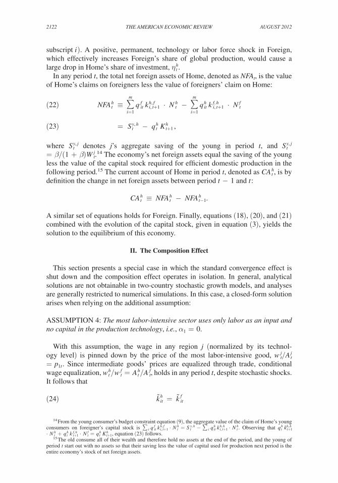
In any period t, the total net foreign assets of Home, denoted as NF A t , is the value of Home’s claims on foreigners less the value of foreigners’ claim on Home:

(22) NF A t h ≡ ∑ i=1

m

q it f k i, t+1 h, f

⋅ N t h − ∑ i=1

m

q it h k i, t+1 f, h

⋅ N t f

(23) = S t y, h − q t h K t+1 h ,

where S t y, j denotes j’s aggregate saving of the young in period t, and S t y, j = β/(1 + β) W t j .14 The economy’s net foreign assets equal the saving of the young less the value of the capital stock required for efficient domestic production in the following period.15 The current account of Home in period t, denoted as C A t h , is by definition the change in net foreign assets between period t − 1 and t :

C A t h ≡ NF A t h − NF A t−1 h .

A similar set of equations holds for Foreign. Finally, equations (18), (20), and (21)combined with the evolution of the capital stock, given in equation (3), yields the solution to the equilibrium of this economy.

II. The Composition Effect

This section presents a special case in which the standard convergence effect is shut down and the composition effect operates in isolation. In general, analytical solutions are not obtainable in two-country stochastic growth models, and analyses are generally restricted to numerical simulations. In this case, a closed-form solution arises when relying on the additional assumption:

ASSUMPTION 4: The most labor-intensive sector uses only labor as an input and no capital in the production technology, i.e., α 1 = 0.

With this assumption, the wage in any region j (normalized by its technol-ogy level) is pinned down by the price of the most labor-intensive good, w t j / A t j = p 1t . Since intermediate goods’ prices are equalized through trade, conditional wage equalization, w t h / w t f = A t h / A t f , holds in any period t, despite stochastic shocks. It follows that

(24) k it h = k it f

14 From the young consumer’s budget constraint equation (9), the aggregate value of the claim of Home’s young consumers on foreigner’s capital stock is ∑ i

q it f

k i, t+1 h, f ⋅ N t h = S t y, h − ∑ i

q it h

k i, t+1 h, h ⋅ N t h . Observing that q t h k t+1 h, h

⋅ N t h + q t h k t+1 f, h

⋅ N t f = q t h K t+1 h , equation (23) follows.

15 The old consume all of their wealth and therefore hold no assets at the end of the period, and the young of period t start out with no assets so that their saving less the value of capital used for production next period is the entire economy’s stock of net foreign assets.


for all i > 1, where k it j = K it j

/( A t j N it j ) is j’s effective capital-labor ratio in sector i.

Labor reallocation across sectors alone is sufficient to equalize sector-level capital effective-labor ratios, across countries. The force of convergence that induces cross-border capital flows to serve this very purpose is effectively shut off.

Now consider a high ϵ N, t f (labor force boom) or ϵ A, t f

(productivity boom) in Foreign. The rise in aggregate wage income accrues to the young consumers, who are the savers in the economy. This leads to a rise in aggregate saving in Foreign. How would Foreign allocate its marginal unit of savings? Since the rental earned from the production technology, α i p i ( k i

j ) α i −1 , is equalized across countries for all periods, Foreign will allocate it to both countries, the amount of which is determined by adjustment costs. With the convergence effect shut off, the country with the labor force/productivity boom will always allocate part of its savings abroad, and thus see an immediate capital outflow.

These results can be shown analytically. Recall that determining Home’s invest-ment in period t amounts to knowing its share in global investment η t , given by equa-tion (22), along with equation (20) and (21).

PROPOSITION 1: With Assumptions 1−4, the share of Home’s investment in any industry i, η it , is a constant and is equal to its initial share of world capital stock in that sector,

η it = K i0 h _ K i0 g ∀t.

PROOF: See Appendix Section IB.With goods trade, Home can expand its capital-intensive sectors and export their

goods in response to a labor force/productivity boom in Foreign. Consequently, the returns to capital in its capital-intensive sectors rise in Home and greater investment demand induces higher capital inflows from abroad.16

Adjustment costs pin down the amount of saving apportioned to each country.17 If countries were initially symmetric, one half of Foreign’s savings would be allo-cated to Home, the remaining half invested domestically. If, however, Home started out with a higher initial aggregate capital stock, K 0 h , the marginal adjustment costs paid to augmenting capital stock in any sector would be lower in the Home country. Home thus commands a greater share of global savings, the constant of proportion-ality being the share of Home’s initial capital stock in global initial capital stock. Note that the result that Foreign allocates part of its savings to Home stems from their ability to trade, and not from adjustment costs, which merely determines the exact quantity.18 In the one-sector model with adjustment costs, the result looks very

16 The rental earned from the intermediate-goods production technology, α i p i ( k i j ) α i −1 , rises for all i ≠ 1.

17 Adjustment costs are proportional to I i j / K i j , which, when equalized, implies that the aggregate investment ratio between country j and k are equal to their capital stock ratio.

18 It is important to note that the role of adjustment costs in this model is merely to pin down the stock of capital, rather than aid the composition effect. Jin and Li (2011) show that in a stochastic, incomplete-markets model, FPE doesn’t hold in this two-sector model with capital mobility as a result of risk. With this scenario, they show that the composition effect operates in the absence of adjustment costs, and still dominates the resource shifting effect.


different as Foreign not only allocates its domestic savings locally but also imports capital from Home, the reason being that capital is more productive in Foreign.

Using equations (17), (21), and Proposition 1, country j’s aggregate investment at t, I t j = η t j I t g can be written as

(25) I t j = ∑ i=1

m

μ i η i0 j ψ s l Y t g .

A positive labor force/productivity shock in any country raises world output at t and thus also raises investment globally, in such a way that more investment is allocated to the country that has a higher initial, weighted-average capital share. In this special case with international trade linkages, investment comoves across countries.

A. Aggregate Savings and Investment

Comparison of the rate of returns across countries is one way of understanding the allocation of savings across countries. An alternative way is by analyzing a coun-try’s supply of saving relative to its demand for investment, which in a multi-sector setting becomes linked to its industrial structure. It is informative to first examine the behavior of labor income in relation to a country’s domestic GDP. This share is constant in the one-sector case, but is no longer constant in a multi-sector case and depends on the comparative advantage of the economy and its production struc-ture. Let k t

j = K t j / N t j be j’s aggregate effective capital-labor ratio in period t, where K t j = ∑ i

K it j

and N t j A t j N t j . And let k t g = K t g / N t

g be the world effective capital-

labor ratio, where K t g = ∑ j K t j and ˜ N t

g = ∑ j

N t j . Then, country j’s relative

capital-effective labor is κ t j = k t j / k t

g , which reflects its own comparative advantage.

A fall in κ t j , due to a high ϵ N, t j or ϵ A, t j

that increases j’s effective labor force at t, causes j to see a greater comparative advantage in labor. Country j’s labor income-GDP ratio can then be expressed as

(26) W t j _

GD P t j = 1 __

κ t j ( s k _ s l + β(1 − ϕ) _ 1 + β )+ 1

.

A fall in κ t j causes j to specialize in labor-intensive goods, a production shift which raises the share of domestic GDP that is accrued to wage income. Thus, the labor share of GDP rises with a fall in the country’s relative capital-labor ratio.

It becomes apparent that in an OLG model, country j ’s saving to GDP ratio at t also depends on its relative capital-labor ratio at t. Since the young, who work and earn labor income, are the savers in the economy, a country’s supply of savings derives from its capacity to generate labor income. A country whose production structure is heavily tilted toward capital-intensive industries inevitably has a small labor income share of domestic GDP, and a low savings rate. On the other hand, a


country which has an industrial structure concentrated on producing labor-intensive goods is able to generate a large share of wage income relative to output. Thus, the saving to GDP ratio in j is also a negative function of κ t j :

(27) S t y, j

_ GD P t j

= β/(1 + β) __ κ t j ( s k _ s l + β(1 − ϕ) _

1 + β ) + 1

.

Likewise, a country which has a comparative advantage in capital (a high κ t ) sees a high share of GDP accrued to investment—and the investment-GDP ratio is a posi-tive function of κ t :

(28) I t j /ϕ _

GD P t j = κ t j [ β/(1 + β)] __

κ t j ( s k _ s l + β(1 − ϕ) _

1 + β ) + 1

.

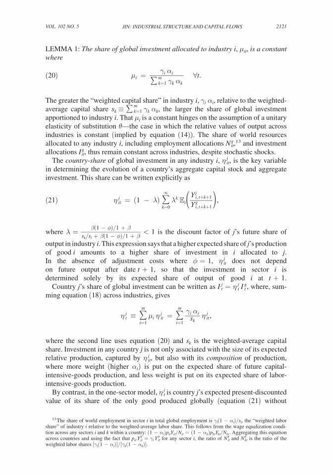
One can now map these saving and investment relationships to an economy’s stock of net foreign assets accumulated over any period t. Recall from equation (23) that the difference between the saving of the young at t, S t y, j , and the market value of capital used for efficient production, I t j /ϕ, is the economy’s value of net foreign assets accumulated by the end of period t, denoted NF A t . Figure 1 displays these two schedules, and shows that they intersect at the point where countries’ capital-labor ratios are equalized—where domestic saving provided by the young of that economy is just enough to serve its domestic investment needs, and no foreign assets need to be accumulated. A positive shock that reduces j’s relative capital-labor ratio at t, leads to a compositional shift that causes its supply of savings to rise by more than its investment demand, the difference showing up as an increase in the stock of net foreign assets, and therefore a capital outflow.

Similarly, one can graph the savings and investment curves in the one sector model. In this case, the investment-GDP curve is downward sloping, as drawn in the second panel of Figure 1. Lower capital effective-labor ratios in any country j requires greater investment in j so that this ratio eventually converges across countries. On the other hand, the savings rate is a constant when Assumptions 1 (log utility) and 2 (θ = 1) are made. In contrast to the multi-sector model, j sees a reduction in its net foreign asset position and a net capital inflow as its capital-labor ratio falls.

These two figures depict the savings-investment relationship when the composi-tion effect and the convergence effect are each respectively isolated. The striking difference is the slope of the investment demand curve, which is negative in the one-sector case but positive in the multi-sector case. In the general case, where both composition and convergence effects coexist, the investment-output curve lies somewhere in between—and becomes positively sloped when the composition effect is stronger and negatively sloped when the convergence effect is stronger. The important factors governing the relative strength of the two effects are dis-cussed in Section IIID.


0.6 0.7 0.8 0.9 1 1.1 1.2 1.3 1.4

0.13

0.14

0.15

0.16

0.17

0.18

0.19

0.2

0.21

Relative capital labor ratio

Sav

ing,

inve

stm

ent s

hare

of G

DP

Multiple sector case (composition effect only)

S

I

NFA

0.6 0.7 0.8 0.9 1 1.1 1.2 1.3

0.102

0.104

0.106

0.108

0.11

0.112

0.114

Relative capital labor ratio

Sav

ing,

inve

stm

ent s

hare

of G

DP

One sector case (convergence effect only)

S

l

Figure 1. S y,j /GDP and I j /(ϕGDP) as a Function of κ t j = k t

j / k t g

Notes: The difference between the savings curve and the investment curve is the country’s net foreign asset position. A reduction in the net foreign asset position amounts to a net capital inflow. The top panel shows the multiple sector case, based on closed-form solutions. It assumes that α 1 = 0, α 2 = 0.1, α 3 = 0.29, α 4 = 0.85, γ i = 0.25 for all i. The bottom panel shows the sim-ulated results of the one sector case, based on equation (21) when i = 1; α 1 = 0.3. In both cases, β = 0.67 and ϕ = 0.5 in this two-period model, in which a period is 20 years.


B. International Capital Flows

The direction of capital flows as a consequence of globalization or labor force/productivity shocks can be summarized by the following propositions:

PROPOSITION 2 (Globalization): Suppose that all countries are initially in autarky prior to period t, and unexpectedly open up to trade and capital flows at t. Then, c a t j > 0 for κ t j < 1.

PROOF:Suppose that the two economies are initially in autarky and liberalize in

period t. The current account (as a share of GDP) in period t for country j is

c a t j = β/(1 + β)(1 − κ t j ) __ κ t j ( s k _ s l + β(1 − ϕ) _

1 + β ) + 1 , where s l < 1. This follows from the net foreign assets

being zero prior to t, and from the definition of the current account, equation (23), using (27) and (28). This shows that c a t j > 0 if and only if κ t j < 1, i.e., if the capital-effective-labor ratio is lower in country j relative to that of the world.

In this model, trade and financial liberalization cause capital to flow from a poor country with a low capital-effective-labor ratio to a rich country with a high capital-effective-labor ratio.

PROPOSITION 3 (Labor Force/Productivity Shock): Suppose that all countries are open at t. A high ϵ A, t j

or ϵ N, t j in country j causes a net capital outflow in j, at t. That

is, d(nf a t j ) _

d( ϵ x, t j ) > 0, where x = A, N.

PROOF:In an open economy, the net foreign assets (as a share of GDP) in period t is

nf a t j = β/(1 + β)(1 − κ t j ) __ κ t j ( s k _ s l

+ β(1 − ϕ) _ 1 + β ) + 1

. By definition, κ t j ≡ k t j / ∑ j

k t

j and k t j

= K t j /( A t−1 j N t−1 j

⋅ e ϵ A, t j + ϵ N, t

j ). Since K t j is fixed in period t, a high ϵ A, t j or ϵ N, t j

reduces k t

j and κ t j . As d(nf a t j )/d( κ t j ) < 0, a positive labor force/productivity shock leads to an increase in net foreign assets, and hence an improvement in the current account.

The evolution of the effective aggregate capital-labor ratio in region j is character-ized by:

(29) ln( k t+1 j ) = ln Θ + (1 − ϕ s l )ln( k t

j ) + ϕ s l ln( ∑ i

μ i η i0 j )

+ ϕ s l (ln ˜ N t g − ln ˜ N t j ) − ( ϵ N, t+1 j

+ ϵ A, t+1 j ),

where Θ is a constant.19 This implies the following proposition:

PROPOSITION 4 (Path Dependence): The evolution of the k t j depends on j’s ini-

tial weighted-average share of capital stock in the world, ∑ i μ i η i0 j

: the higher the

19 Θ = a(ψ s l / s k ∏ i=1 m γ i γ i ( α i γ i ) α i γ i [(1 − α i ) γ i ] (1− α i ) γ i ) ϕ .


initial weighted-average share of capital in j, the higher the effective capital-labor ratio in j at every point on the transitional path.

The country with the higher initial capital stock commands lower marginal adjust-ment costs paid on investment in that country, and thus commands a higher share of world investment.

III. Quantitative Analysis

This section explores the quantitative implications of the general framework in which both the composition effect and the convergence effect coexist. It extends the analytical two-period OLG framework to a multi-period OLG setting, allow-ing for an additional nontradable sector. The quantitative framework is applied to two important global events in the past decades. The first is the integration of China, India, and the ex-Soviet bloc into the world economy in the beginning of the 1990s. The experiment examines what the almost-simultaneous advent of these emerging economies (henceforward E-countries) implies for international capital flows. The second experiment is motivated by the observation that developing countries as a whole have experienced a rapid increase in the labor force, compared to advanced economies over the period 1990–2010. While the working age popu-lation (ages 25–59) in developing countries grew by an average five-year growth rate of 12.7 percent over this period, it grew at a much slower rate of 2.97 percent in advanced economies.20 The vast asymmetry in the labor force growth rate has spurred interest in its impact on the current account, but none of the existing studies on this topic take into account factor-proportions trade.21 At the same time, many of the developing economies experienced rapid productivity growth, leading to an average five-year growth rate in GDP per capita of 3.28 percent in the region com-pared to 2.29 percent in the developed region, over the same period.

A. A Multi-Period OLG Model

To investigate the quantitative relevance of the multi-sector framework developed in this paper, I extend it to a multi-period OLG model following Auerbach and Kotlikoff (1987). Agents in country j = h, f live for T periods and supply one unit of labor each period, during the first J periods of their life, after which they retire. They are born with zero wealth and cannot die with negative wealth. Preferences are CRRA as before, where

u j = ∑ t=1

T

β t (( c t j ) 1−ρ − 1)/(1 − ρ).

20 These statistics are taken from the World Population Prospects: The 2010 Revision. The developed econo-mies comprise all regions of Europe plus Northern America, Australia/New Zealand, and Japan. The less devel-oped economies comprise all regions of Africa, Asia (excluding Japan), Latin America, and the Caribbean plus Melanesia, Micronesia, and Polynesia.

21 See Boersch-Supan, Ludwig, and Winter (2005); Attanasio, Kitao, and Violante (2007); and Fehr, Jokisch, and Kotlikoff (2006).


Each agent’s lifetime budget constraints requires that

∑ t=1

T

( ∏ s=1

t

R s −1 ) c t j = ∑ t=1

J

( ∏ s=1

t

R s −1 ) w t j ,

where w t j is country j’s wage rate in period t, and R t is the rate of return in period t. The production side is the same as before.

Nontradable Goods.—Since nontradable goods comprise a large share of an economy’s output, I incorporate a domestic nontradable sector in each country into the existing framework. Country j’s consumption index becomes

(30) C t j = [ γ T 1 _ ζ ( C T, t j

) ζ−1

_ ζ + (1 − γ T ) 1 _ ζ ( C N, t j

) ζ−1

_ ζ ],where C N, t j

and C T, t j denote j’s aggregate consumption of the nontraded good

and the composite tradable good, which, as in equation (12), takes the form

C T, t j = [ ∑ i=1

m γ i

1 _ θ ( c it j )

θ−1 _ θ ] θ _ θ−1

. Only the composite tradable good can be used for

investment. The overall consumer price index becomes

(31) P t j = [ γ T ( P T, t j ) 1−ζ + (1 − γ T )( P N, t j

) 1−ζ ] 1 _ 1−ζ ,

where P T, t j is the same as equation (2), and is normalized to 1. In equilibrium, both

p it and the relative price of nontraded to traded goods in j at t, P N, t j , are determined

endogenously. Let the gross output of the nontraded good in country j be

(32) Y Nt j = ( K Nt j

) α N ( A t j N Nt j ) 1− α N ,

where K Nt j is the aggregate capital stock in the nontraded sector, and N Nt j

is the labor used in the nontraded sector in j, at t. The additional market clearing condition of the non-traded sector requires

(33) Y N, t j = C N, t j

,

that the output of nontradable goods in j must equal the domestic consumption of that good. The domestic labor market clears when ∑ i=1

m N it j

+ N Nt j = N t j .

B. Calibration

Specialization and industrial restructuring takes time and so the appropriate time frame for this model is one of medium-low frequency. As such, one period is cho-sen to be five years. Since the framework builds on the neoclassical growth model, most of the parameters are standard, provided in Table 1. The regions in the first


quantitative experiment correspond to China, India, and the Soviet-bloc (E-region) against the rest of the world (ROW), and advanced economies (Home) versus devel-oping countries (Foreign) in the second quantitative experiment.

Preferences.—Agents enter the economy at age 25 and work until age 59, after which they live until age 80. The intertemporal elasticity of substitution is set to the standard value ρ = 2. The discount factor on an annual basis is set to 0.98 which yields β = 0.9 over a five-year period.

Factor Intensities and Other Parameters.—The baseline model takes the bench-mark case of a unitary elasticity of substitution among tradable goods, θ = 1, which implies that γ i ’s are equal to the share of sector i in the world’s total value added. Estimates of factor intensity shares ( α i ’s) and share of value added ( γ i ’s) for 28 sectors in the OECD Annual National Accounts Table are provided in Cuñat and Maffezzoli (2004). Among the 28 sectors, 18 can be categorized as tradable goods, following the classification in Stockman and Tesar (1990). I rank the sectors by their capital intensity and assume that the first nine sectors are labor-intensive, and the other nine sectors capital-intensive. The capital shares are respectively denoted as α l and α c . The share of the labor-intensive sector in total value added, γ l , is then chosen such that γ l = ∑ i=1

9 γ i . Factor shares α l and α c are calibrated to match the weighted-

mean of the capital share of the 18 sector, s k = ∑ i=1 18

γ i α i = 0.31, and the weighted variance ∑ i=1

18 γ i ( α i − s k ) 2 = 0.04, which capture the degree of factor intensity

differences across sectors. The resulting parameterization is γ l = 0.4, γ c = 0.6, α l = 0.11, α c = 0.52.22 Following Stockman and Tesar (1990) and Coeurdacier (2009), γ N is calibrated to match the average share of nontradable goods in total consumption expenditure, which is 55 percent. This gives γ T = 0.45. The existing literature focuses on low values of ζ, ranging from 0 to 1 for industrialized countries (see Coeurdacier 2009), and thus ζ = 0.55 is chosen as in Stockman and Tesar (1990). The overall weighted mean of the labor share for all 28 sectors is 0.65. The labor share α N is calibrated to match the weighted mean of the labor share for all of the 10 nontradable sectors, which gives α N = 0.6.

The drawback of the log-linear capital adjustment function is that deprecia-tion and adjustment costs, both of which are captured by the parameter ϕ, cannot

22 In this calibration, a two-sector case is considered rather than a multi-sector case. What matters the most for the qualitative and quantitative results is the dispersion of factor intensity, discussed in detail in Section IIID. In a two-sector model, the factor intensity dispersion is matched to that of the data, which features 18 tradable sectors. Extending the model to a 5-sector setting yields similar results, and is omitted in the text.

Table 1—Parameters

Benchmark parameter values

Preferences β = 0.9 γ l = 0.4, γ c = 0.6 γ T ∈ {0.42, 1} ζ = 0.45

ρ = 2 θ = 1Technology α l = 0.11, α c = 0.52 α N = 0.6

b = 0.8 δ = 0.226


be separated. Therefore, the standard capital-adjustment model, equation (4), is henceforward adopted in the quantitative exercises. The depreciation rate of capital is assumed to be 5 percent per year in both regions, implying a value of δ = 0.226. Capital adjustment costs are widely used but there is no consensus on the calibration strategy to parameterize them.23 The adjustment cost parameter b can range any-where from 0.3 to 20. The strategy adopted in this model is to match the timing of adjustment in this five-year/period model with that of an annual frequency model, where the adjustment cost parameter in the annual model is selected based on the approach of the international real business cycle. That is, b is first chosen in an annual-frequency model to match the relative volatility of investment generated by a two-country multi-sector business cycle model, following the standard literature.24 Using this standard annual-based calibration of the adjustment cost parameter, b is then chosen, in the current five-year-period model, so that the amount of capital adjustment that takes place in the annual frequency model, over five years, is the same amount that takes place over one period in the current model. In the baseline experiment, this gives a value of b = 0.8. Admittedly, no calibration technique of the adjustment cost parameters will be entirely satisfactory, although the sensitivity analysis in Table 6 shows that the qualitative results are insensitive to the size of the adjustment costs, and that the quantitative results are driven to a much larger extent by factor intensity differences than by adjustment costs.

Relative Size and Technology.—According to the U.N. population statistics, the ratio of the total population of E-countries to the rest of the world in 1990 is 0.68. The initial technology ratio between these two groups of countries is chosen to match the GDP per capita ratio between ROW and E-countries, which is about 11.88, accord-ing to the World Development Indicator. This gives an initial technology ratio of 2.9, which implies a capital-labor ratio in ROW of about 5 times that of E-countries. Similarly, for advanced economies versus developing countries as a whole, the tech-nology ratio is set to 2.14.25 I allow TFP in the E-region to gradually converge to the level of the ROW by 2050. All other parameters are provided in Table 1.

C. Results

Scenario 1 (Integration of China, India, and the ex-Soviet Bloc): Countries are assumed to be initially in their autarkic steady states. In the first

period, corresponding to the year 1990, the E-region unexpectedly opens up to both trade and financial capital flows. The transition path is computed according to the algorithm described in Appendix Section II. Characterized by an initially low TFP and low capital-labor ratio, its autarky price of labor-intensive goods (good 1) is depressed relative to the international price (see Appendix Section III). Thus, from

23 For example, Baxter and Crucini (1995) calibrates the elasticity of investment relative to Tobin’s q to match investment variability in industrial countries. Chari, Kehoe, and McGrattan (2001) calibrates the parameter to match the relative variability of consumption to output. Kehoe and Perri (2002) targets the variability of investment.

24 This value is taken from Jin and Li (2011), which calibrates a two-country multi-sector international business cycle model. The only departure of this model from the workhorse framework of Backus, Kehoe and Kydland (1992) is the addition of a tradable sector (differing in factor intensity).

25 The initial steady-state equilibrium on which these calibrations are based is described in Appendix Section III.


the perspective of E-countries, the price of good 1 increases on impact when open-ing up to trade. As Table 2 shows, in the absence of a nontradable sector, this price increases by 9.48 percent in the first period, while the price of the capital-intensive good falls by 5.86 percent. On the other hand, trade integration allows ROW to see a reduction in its price of labor-intensive goods on impact and a rise in the price of capital- intensive goods. Consequently, E-region with a comparative advantage in labor specializes in labor-intensive goods and runs a large initial current account surplus of 17.07 percent of GDP, subsequently reverting to balance after 2020. ROW runs an initial current account deficit of 3.73 percent of GDP.

The incorporation of the nontradable sector reduces the impact of trade and spe-cialization on capital flows without changing the results qualitatively. The rise in the wage in the E-region pushes up the price of the nontradable good, leading to a real appreciation, while the opposite occurs in the ROW. This result resonates with the Balassa-Samuelson effect although the instigation of the real appreciation in developing economies in this case is brought about by globalization, rather than by faster productivity growth in the tradable sector. The expansion of all sectors, including the nontradable sector, requires E-countries to invest more of its saving domestically, thus reducing the amount of capital released to ROW. On average, E-countries run a current account of 6.09 percent of GDP between 1990–2010, and ROW an average deficit of 1.35 percent of GDP, compared to the average surplus of 3.15 percent of GDP and − 0.45 percent of GDP, respectively, in the data (Table 2).

Table 2—Quantitative Analysis: Integration of E-Countries

1990–1994 1995–1999 2000–2004 2005–2009 2010–2014 2015–2020

Data: current account ( percent of GDP)E-countries 1.02 1.35 3.25 6.98ROW −0.29 −0.31 −0.64 −0.59

Only tradablesCurrent account ( percent of GDP) E-region 17.07 15.13 12.89 10.24 7.03 3.05 ROW −3.73 −3.21 −2.67 −2.07 −1.40 −0.6

Trade balance ( percent of GDP) E-region 17.07 11.48 5.92 0.38 −5.16 −10.79 ROW −3.73 −2.43 −1.22 −0.08 1.03 2.12Prices (percent deviation) p 1

e 9.48 9.56 9.65 9.75 9.84 9.91

p 2 e −5.86 −5.91 −5.96 −6.01 −6.06 −6.11

p 1 row −1.91 −1.84 −1.76 −1.68 −1.59 −1.53

p 2 row 1.29 1.25 1.19 1.13 1.08 1.03

Adding nontradable sectorCurrent account (percent of GDP) E-region 8.05 6.93 5.54 3.82 1.68 −0.99 ROW −1.81 −1.55 −1.23 −0.84 −0.37 0.22

Trade balance (percent of GDP) E-region 8.05 5.24 2.39 −0.51 −3.47 −6.49 ROW −1.81 −1.17 −0.53 0.11 0.76 1.42

Price of nontradable good (percent of deviation) E-region 5.43 5.74 6.10 6.52 7.03 7.70 ROW −0.89 −0.92 −0.91 −0.85 −0.77 −0.67

Note: This table reports the current account as a percentage of GDP, and percentage deviations of goods prices from their initial levels, both in the case with only tradable goods, and the case with an additional nontradable good.


Scenario 2 (Effective Labor Force Growth in Developing Countries):Next the impact of faster labor productivity/force growth in developing countries

on global imbalances can be evaluated in the same framework. Labor force growth is taken to be the growth of the working age population (ages 25–59) (Table 3), and labor productivity growth is set to match the average GDP per capita growth over 1990–2010, in both regions.

As shown in Table 3, developing countries run an initial small current account deficit between 1990–1994, followed by a current account surplus in all remaining periods. The results are modest compared to the previous experiment (Scenario 1) because the changes in the effective labor force, except during the first period, are assumed to be fully anticipated. Developing countries will at least to some extent start accumulating capital in anticipation of the labor force/productivity growth. This tends to reduce the difference in the capital-labor ratio across countries at the time of the shock, and hence the extent of comparative advantage. Therefore, less capital flows out of developing countries. To the extent that some labor force/pro-ductivity changes are unanticipated, the current account would respond by a greater margin. Therefore, these results can be interpreted as a lower bound of the amount of capital released from developing to advanced economies due to asymmetric effective labor force growths. Overall, the integration between a capital-poor devel-oping country and a capital-rich advanced economy can be seen to be a much more quantitatively important factor in accounting for global imbalances than differences in labor force/productivity growth rates.

These results are brought into stark contrast with those emerging from the one-sector model. As shown in Table 3, developing countries now run a large current

Table 3—Quantitative Analysis: Faster Labor Force/Productivity Growth in Developing Countries

1990–1994 1995–1999 2000–2004 2005–2010 2010–2015 2015–2020

Data: current account ( percent of GDP) Developing −1.37 −1.20 1.00 2.79 Advanced −0.22 0.01 −0.70 −0.66

Working-age population growth ( percent) Developing 15.10 13.47 11.32 10.79 Advanced 4.08 2.79 3.59 1.42

Two sectors: only tradablesCurrent account (percent of GDP) Developing −1.42 0.49 3.08 5.92 8.72 11.75 Advanced 0.63 −0.25 −1.91 −4.26 −7.22 −11.03

Adding nontradable sectorCurrent account (percent of GDP) Developing −0.70 −0.31 0.02 0.31 0.34 0.35 Advanced 2.80 1.27 0.10 −1.32 −1.50 −1.52

One sector: only tradablesCurrent account (percent of GDP) Developing −39.14 −27.52 −20.96 −16.52 −13.76 −10.84 Advanced 13.52 13.28 13.13 12.95 13.25 12.76

Notes: This table reports developing and advanced countries’ current account as a percentage of GDP, for the case with only tradable goods, and the case adding a nontradable good. It contrasts the results of a multi-sector case with those of the one-sector case.


account deficit in every period, while advanced economies run a surplus. In this case, with only the convergence effect determining capital flows, the direction of the flows is toward developing countries where capital is more productive. The results are very large and point to precisely the fact that rapid growth in emerging countries should lead to a massive influx of capital—according to the standard model. Adding a non-tradable sector leads to negligible differences and thus omitted from this analysis.

D. Discussion

Comparison with Infinite-Horizon Models.—Do the main results hold when mov-ing away from an OLG model to an infinite-horizon model? The impact effect of these shocks on the economy is the same across the two models, and hence special-ization patterns at the time of the shock are identical. For this reason, the composition effect—the rise in demand for capital in the country that has shifted its production toward more capital-intensive sectors—still exerts its force on determining capi-tal flows. In other words, investment demand behaves similarly in the two models. However, savings behavior differs, and hence affect quantitatively the amount of capital that can be released from the country with the positive labor force/productiv-ity shock. In an OLG framework, aggregate savings rises by more than in an infinite-horizon model in the country with the boom. This tends to increase the amount of capital than can be released abroad. For this reason, anything that increases the amount of aggregate savings during booms in one country—for example, borrowing constraints—can raise the amount of net capital outflows away from that country.

Strength of the Composition Effect.—In the general model, where the composi-tion effect and the convergence effect are competing, the “reversal’’ of capital flows relies on the composition effect outweighing the convergence effect. The composi-tion effect is strong when specialization patterns are pronounced, and the extent of specialization critically depends on factor intensity differences across sectors. In the limit where factor intensities converge to the same level, the multi-sector model yields qualitatively similar results to a one-sector model. As factor intensities become more disparate, the composition effect becomes stronger.26

Other Parameters.—Following on the intuition provided above, the key parameters determining the magnitudes of the current account responses are to a much larger extent governed by factor intensity differences. The size of the adjustment costs, b, and the elasticity of substitution θ, along with other parameters, can affect the results quantitatively although not qualitatively. Since the trade structure of this economy is one of incomplete specialization, θ plays a much less important role than in the case where countries specialize in differentiated goods. To demonstrate this simply, Table 6 reports sensitivity analyses in the baseline experiment where one of the two ex ante identical countries, Foreign, experiences a permanent labor force boom. The results

26 In a multi-tradable goods setting, a measure of the dispersion of factor intensities is the weighted-variance of α i : ∑ i=1

m γ i ( α i − s k ) 2 . Estimated from the OECD data with 18 tradable sectors, the weighted-mean of capital

intensity, s k , is 0.31, and the weighted variance is 0.04. The experiment that holds fixed the weighted-mean s k while increasing the weighted-variance shows that capital flows away from the country with the boom increases with the dispersion of factor intensities. These results are not presented but are available upon request.


show Home’s current account response on impact. Reducing the size of adjustment costs induces a larger current account deficit as the amount of desired investment increases. Experiment (2) and (3) show that qualitatively, the current account always falls for Home, so long as factor intensities are sufficiently different. Moreover, vary-ing the elasticity of substitution θ and the risk aversion parameter ρ makes very little difference in impacting the current account. A low elasticity of substitution engenders a greater increase in the price of the capital-intensive good than in the high elastic-ity case. This can lead to a greater demand in capital for Home, although the effect is small. While changing ρ has some impact on the amount of saving generated by Foreign, it has very little material consequence on the results of interest as investment demand is the quantitatively (and qualitatively) dominant force.

IV. Suggestive Empirical Evidence

The studies on the relationship between capital flows and trade flows, ever since the inception of the Heckscher-Ohlin-Mundell framework, have remained principally theoretical inquisitions. Although empirical studies provide evidence that more trade in goods is associated with greater financial asset trade (Portes and Rey 2005 and Aviat and Coeurdacier 2007), the specific channels through which commodity trade impacts capital flows in the data have remained unexplored. Firmly establishing the empiri-cal link between a specific type of trade and a particular direction of capital flows is beyond the scope of this paper. Instead, the purpose of this section is to provide some suggestive evidence for the main prediction of the theory. It first documents facts on the trading patterns and the current account dynamics across countries over the last two decades, and then proceeds to investigate the main prediction of the theory: whether countries which have become more specialized in capital-intensive goods have also run greater current account deficits. In addition, I examine whether changes in the relative prices of capital and labor-intensive goods are consistent with the theory.

The methodology adopted requires two steps: (i) constructing time-varying spe-cialization patterns for each country, based on the notion of “Revealed Comparative Advantage’’, and (ii) using these specialization patterns to detect whether changes in these patterns are correlated with current account movements in a way that is consistent with the theory.

The existing empirical literature on the determinants of the current account does not include the impact of changes in specialization patterns over time.27 In the litera-ture, the notion of “revealed comparative advantage’’ (henceforward RCA) in capi-tal, measures a country’s capital intensity as revealed by trade flows.28 As in Romalis (2004), which uses this measure to examine the relationship between a country’s factor proportions and its structure of trade, the same measure is adopted here, where a country-specific coefficient α j is estimated from the following regression:

(34) x jz = β j + α j ⋅ k z + χ j ⋅ s z + ϵ jz ,

27 See Chinn and Prasad (2003).28 The term “revealed comparative advantage’’ first appeared in Balassa (1965).


where x jz is the share that country j commands of world imports in industry z, k z , and s z are the capital intensity and skill intensity of industry z. Thus α j is the percentage point increase in country j’s market share of z, for each 1-percentage point increase in capital-intensity. Countries can therefore be ranked according to α j .

Factor intensities, k and s, of each industry are calculated using the NBER Manufacturing Industry Productivity Database, which covers 459 industries at the 4-digit SIC level for a period up to 2005. I make the assumption, standard in the literature, that factor intensities of each industry are the same across coun-tries and thus use the US data as a benchmark. Because of data limitations, I also assume that factor intensities have not changed between the year 2005 and 2006, the last year in the sample period. Following Romalis (2004) k is measured as 1 less the share of total labor compensation in value added, and s is measured as the share of nonproduction workers in total employment in each industry. Rather than using countries’ exports to the United States as in Romalis (2004), I adopt the approach of Nunn (2007) and Cuñat and Melitz (2012) in using countries’ exports to the world (data described in Appendix Section III).

Patterns of “Revealed Comparative Advantage’’ and the Current Account.—The RCA of each of the “E-countries’’ (China, India, and Russia), as shown in Table 4, has fallen between the periods 1989–1993 to 2002–2006. For example, each 1-percentage point increase in capital intensity is estimated to reduce China’s mar-ket share by an average of 3.66 percentage points in the period 1989–1993, and by an average of 4.11 percentage points in the period 2002–2006.29

The RCA for developing countries as a whole—that is, all countries with per capita GDP at PPP of not more than 50 percent of the US level in each period—is obtained by performing regression 34 on this group of countries.30 Developing countries’ market share is calculated as x sz = ∑ j∈Developing

x jz for each industry z.

Table 4 reports the results for developing countries over the same sample period. Its market share also falls significantly with the capital intensity of the industry, and that share has been decreasing over time.31

29 China’s labor-intensity of exports steadily increased in the period between 1989 and 2006, possibly as a result of increased trade liberalization that allowed it to specialize and export more in labor-intensive sectors. The sharpest rise in labor-intensity occurred between 1998 to 2002, from α China = − 3.5 to − 4.25, coinciding with China’s joining the WTO in 2000–2001. It is important to note that the current methodology in measuring the labor-intensity of exports possibly underestimates the degree of China’s labor intensity embodied in exports, as a large component of China’s exports has recently become processing trade—the practice of assembling duty free intermediate inputs. These inputs are generally of high skill and capital content, and thus by failing to account for the labor-intensity of assembly, the labor embodied in exports for the case of China is most likely higher than revealed by the trade data.

30 Advanced Economies comprise Australia, Austria, Belgium, Canada, Denmark, Spain, Finland, France, Greece, Hong Kong, Ireland, Iceland, Israel, Italy, Japan, the Netherlands, Norway, New Zealand, Singapore, Sweden, and the United Kingdom.

31 Examining developing countries on an individual basis, most have also seen a decline in the capital inten-sity of exports over this period. Those that have recently contributed the most to the current account surplus are China, Saudi Arabia, Russia, and Iran, all of which have experienced a fall in capital-intensity over this period, accompanied by an improvement in the current account. The countries that have experienced a notable increase in the capital intensity of exports are Bolivia, Korea, Malaysia, Morocco, Thailand, and the Philippines. These Asian countries, which saw a rise in the capital intensity of exports, experienced an improvement in the current account. However, all of these countries experienced a sharp rise in the current account in 1998 during and after the East Asian financial crisis.


Using α j , I then proceed to examine whether there is a systematic relationship between a country’s capital-intensity of exports and the current account in a panel regression model. The regression specification considered is32

(35) C A jt = α + β 1 ⋅ α jt + γ ′ Z jt + u jt ,

where C A jt is the current account to GDP ratio, α jt is country j’s coefficient on capi-tal intensity in period t,33 Z t is a vector of controls, and u jt is a disturbance term. The sample period covers 1989, 1993, 1998, 2002, and 2006. Control variables are taken from the standard literature on the determinants of the current account, provided in both Gruber and Kamin (2007) and Chinn and Prasad (2003). These include per capita income, GDP growth rate, demographic variables (population growth and the share of working age population to total population), openness, and capital controls. Following Forbes (2010), I also include a measure of financial development as mea-sured by the ratio of stock market capitalization to GDP.

Panel regression estimates are presented in Table 5. The central theoretical predic-tion is that countries which become more specialized in capital-intensive industries over time run greater current account deficits. For this reason, fixed-effects panel regressions are reported in columns 1– 4. The coefficients are negative and signifi-cant. A 1-percentage point higher market share of exports to the world, for every 1-percentage point increase in capital-intensity, is associated with a 0.93-percentage point fall in the current account as a percentage of GDP. When including financial development and capital controls, the negative impact of an increase in capital inten-sity of exports on the current account becomes larger. These fixed-effect regression coefficients suggest that countries that become more capital-intensive over time run higher current account deficits. However, the current analysis does not take into account the possibility that countries’ current account dynamics may vary, and that

32 I assume that the measurement error arising from estimating α jt is uncorrelated with u jt .33 It is derived based on normalized shares of import, x jz , whereby the import share in country j in industry z is

divided by the average value of x jz , so as to make α j comparable across countries.

Table 4—“RCA” and Current Account Dynamics

α j CA (percent of GDP)

E-countriesChina 1989–1993 −3.66 −1.95

2002–2006 −4.11 6.22

India 1989–1993 −2.46 −2.332002–2006 −3.35 0.2

Russia 1989–1993 4.3 2.012002–2006 0.6 9

Developing countries 1989–1993 −0.35 −1.372002–2006 −0.51 2.19

Notes: This table reports the “RCA” in capital ( α j ) and the current account as a share of GDP for a group of developing countries over time. It reports the average of the variables over the initial period, 1989–1993,and the second period, 2002–2006.


Table 5—“RCA” in Capital Intensity and the Current Account

(1) (2) (3) (4 )

Capital intensity −0.929*** −0.940*** −0.823*** −1.228*(0.23) (0.23) (0.22) (0.73)

Openness 2.973 3.540* 6.055*** 6.501**(1.98) (2.08) (2.05) (3.04)

GDP growth −0.210*** −0.224*** −0.246*** −0.472***(0.079) (0.079) (0.081) (0.01)

Population growth −2.558*** −2.475*** −2.204*** −0.773(0.74) (0.76) (0.76) (0.95)

Financial development 1.255(3.13)

Capital controls 1.699(1.17)

Country fixed effects Yes Yes Yes Yes

Year dummies No Yes Yes Yes

Observations 452 452 428 126

R2 0.14 0.18 0.19 0.46

Notes: This table reports the results of estimating C A jt = α + β · α j t + γ ′ Z t + u jt . Column 1 reports results using country fixed effects and column 2 reports those using country and year fixed effects. Column 3 reports results when oil producing countries are omitted (see Appendix Section III). Constants, country and the interaction term between β and the control variables, year effects, are not reported. The sample consists of the years t, 1989, 1993, 1998, 2002, 2006, for all countries. Additional controls include GDP, GDP per capita, and the share of working age population.

*** Significant at the 1 percent level. ** Significant at the 5 percent level. * Significant at the 10 percent level.

Table 6—Sensitivity Analysis

Two-sector CA (percent)

(1) Varying adjustment costsb = 0.1 −1.12 b = 0.3 −1.05b = 0.5 −0.98

(2) Varying factor intensity α c / α l = l 5.01 α c / α l = 3 −0.84 α c / α l = 9 −1.76

(3) InteractionHigh b and high α c / α l −1.37Low b and high α c / α l −1.59High b and low α c / α l −0.95

(4) Elasticity of substitutionθ = 0.8 −1.07θ = 4 −0.86

(5) Risk aversionρ = 0.8 −1.33ρ = 2 −0.96

Notes: A 50 percent increase in the Foreign labor force in the benchmark two-period model. Home and Foreign are ex ante identical. The results are the response of Home’s current account on impact. Experiment 1 varies b from 0.1 to 0.5, while holding constant other parameters in Table 1; 2 holds constant all parameters except the factor intensity ratio, α c / α l . The levels of α c and α l are obtained by fixing the weighted mean γ α l + (1 − γ) α c = 0.31 and setting their ratio to each of the values above; 3 explore interactions between b and α c / α l .


there may be other omitted variables that are correlated with the capital-intensity of exports and also affect the current account.

Relative Prices.—Finally, I show that the requisite fall in the price of labor-intensive goods, as predicted by the model, is met by the data covering the period 1990–2006. To construct this relative price, 39 sectors taken from data provided by the Bureau of Economic Analysis (BEA) are aggregated into one labor-intensive and one capital-intensive sector. The price for each aggregated sector is found by dividing the nominal sectoral value-added by the real sectoral value-added. Figure 2 displays the relative price of labor-intensive to capital-intensive goods. Overall, there is a significant downward trend, amounting to a 11.5 percent decrease between 1989–2006, with the sharpest decline occurring in the 1990s.

V. Final Remarks

International commodity trade and financial capital flows are inherently intertwined in the process of globalization, yet the workhorse international-macro model has neglected to analyze them jointly. The capital-intensity of a country’s export and pro-duction structure affects its demand for financial capital, and financial capital inflows into a country can affect its degree of specialization in capital-intensive industries. This interaction is key to determining global allocations of capital. A simple and yet more realistic enrichment of the standard model to include multiple sectors thus com-pels us to reassess the way a variety of shocks impinge on the world economy.

In the framework that I develop, a novel force emerges, coexisting with the convergence force in shaping global capital flows: capital tends to flow toward countries that become more specialized in capital-intensive sectors. This implies that the integration of developing countries into the world economy, or faster labor force/productivity growth therein can lead to capital flows away from these countries. This stands in sharp contrast to the prediction of the standard one-sector model, but is more consistent with patterns in the data.

Relative price of labor-intensive goods

0.95

1

1.05

1.1

1.15

1985

1987

1989

1991

1993

1995

1997

1999

2001

2003

2005

2007

2009

Figure 2. The Relative Price of Labor-Intensive to Capital-Intensive Goods Over Time (Annually, 1985–2009)


The result that a labor force/productivity boom in one country can drive up invest-ment globally depends critically on the extent of financial and trade integration of world economies. Impediments to the free flow of goods and capital among coun-tries, along with rising protectionism in certain parts of the world, will inevitably compromise the economies’ ability to share these shocks globally. But if greater interdependence is the direction toward which the world is heading, a synthesized framework that takes into account a comprehensive set of forces that shape our inte-grated economy serves a useful purpose in its own right.

Appendix

I. Derivations of the Analytical Model

A. The Two-Country, Two-Period Multi-Sector OLG Model

PROOF OF LEMMA 1:With Assumption 2 (log utility), the optimal consumption for any young con-

sumer in j is

(36) c t y, j = 1 _ 1 + β w t j .

When aggregating the above expression and summing across countries to get aggre-gate global consumption of the young, C t y, g = ∑ j

c t y, j N t j and plugging into the

young consumer’s budget constraint, equation (9), gives world investment

(37) I t g = ϕβ _ 1 + β W t g = ϕβ _

1 + β s l Y t g ,

where I t g = ∑ j ∑ i

I it j

and W t g = ∑ j w t j N t j , and Y t g denotes world nominal output,

∑ i p it Y it g

. The share of wage income in total world nominal output is denoted as s l where s l = ∑ i

γ i (1 − α i ).34 With markets being effectively complete, we have the

efficient allocation condition

(38) C t y _ C t y, g

= C t+1 o _ C t+1 o, g ,

where C t y, j = c t y, j N t j and C t o, j = c t o, j N t j . Aggregating the budget constraint equa-tion (10) and summing across countries gives

(39) C t o, g = ( s k + (1 − ϕ)β _ 1 + β s l ) Y t g ,

34 The assumption of θ = 1 implies that p i Y i g = γ i ∑ i p i Y i g . Therefore, global wage income as a share of world

nominal output W g / ∑ i p i Y i g where W g = (1 − α i ) p i Y i g is therefore the share s l ≡ γ i (1 − α i ). Analogously, the

share of capital income is ∑ i α i p i Y i g is s k = ∑ i

γ i α i = 1 − s l .


where s k = 1 − s l and is the share of capital income in world output. Plugging this expression, along with the total world consumption of the young into the standard Euler equation associated with a Home agent’s household’s problem,

(40) u′( c t y, h ) = β 피 t [u′( c t+1 o, j ) R i, t+1 j

]

for any i = 1, … , m gives

(41) 1 = [ ϕβ _ 1 + β W t g ___

∑ i p i, t+1 Y i, t+1 g

( s k + (1 − ϕ)β _ 1 + β s l ) α i p i, t+1 Y i, t+1 j

+ 1 − ϕ _ ϕ I i, t+1 j ___

I it j ],

where c t y, h / c t+1 o, h = c t y, h N t h /( c t+1 o, h

N t h ) = C t y, g / C t+1 o, g , where the second equality comes

from equation (38). Using the notation I it j = μ it η it I t g and equation (37), the above

expression becomes

(42) μ it η it = 피 t [ α i γ i __

s k + (1 − ϕ)β _ 1 + β s l

Y i, t+1 h

_ Y i, t+1 g

+

(1 − ϕ)β _ 1 + β s l

__ s k + (1 − ϕ)β _

1 + β s l μ i, t+1 η i, t+1 ]

(43) = 피 t [ λ i Y i, t+1 h

_ Y i, t+1 g

+ λ μ i, t+1 η i, t+1 ],

where λ i = α i γ i _

s k + (1 − ϕ)β _ 1 + β s l

, λ = (1 − ϕ)β _

1 + β s l _

s k + (1 − ϕ)β _ 1 + β s l

, and ∑ i λ i = 1 − λ. Summing the

above equation across countries gives

(44) μ it = λ i + λ 피 t [ μ i, t+1 ],

which implies that μ i is a constant. Since μ i = λ i _

1 − λ , it must be that

μ i = α i γ i _ ∑ i

α i γ i

.

Dividing μ i on both sides of equation (42), while using μ = λ i _

1 − λ yields

(45) η it = (1 − λ) 피 t [ Y i, t+1 h _ Y i, t+1 g

] + λ 피 t [ η i, t+1 ]

(46) = (1 − λ) ∑ k=0

∞

λ k 피 t [ Y i, t+k+1 h _ Y i, t+k+1 g

],


which corresponds to equation (21).

B. Special Case: A Closed-Form Solution

PROOF OF PROPOSITION 1:The special case assumes that α 1 = 0, which leads to w t j = A t j p 1t where w t j is the

country-specific wage rate in j. Since goods prices are equalized across countries, this implies that the sectoral capital-effective-labor ratios k it

j are equalized across

countries for all i > 1. Therefore, Y i, t+1 h

_ Y i, t+1

g

= K i, t+1 h _

K i, t+1 g

. The following proof shows that η it

from equation (46) is a constant and equal to K i0 h / K i0 g

:

PROOF:Guess that

K it h _

K it g = η it . Using K i, t+1 = a I it ϕ K it 1−ϕ , and letting I it h

= η it I it g and

I it f = (1 − η it ) I it

g , it must be that

Y i, t+1 h _

Y i, t+1 g

= K i, t+1 h _

K i, t+1 g

= 1 _

1 + K i, t+1

f _

K i, t+1 h

= 1 __

1 + (1 − η it ) ϕ __ η it

ϕ ( K it f ) 1−ϕ _

( K it h ) 1−ϕ

= η it . This shows that if K it h

_ K it

g = η it , it naturally follows that

K i, t+1 h _

K i, t+1 g

= η it . By induction,

K i, t+u+1 h

_ K i, t+u+1

g

= η i, t+u = η i, t+u−1 = … = η i0 , for any u ≥ 0, so that Y i, t+u+1 h

_ Y i, t+u+1

g

= η i0 ∀u ≥ 0.

This implies that η it = λ ∑ u=0 ∞ ( 1 − λ ) k 피 t [ K i, t+u+1 h

_ K i, t+u+1

g

] = λ ∑ u=0 ∞ ( 1 − λ ) u 피 t [ η i0 ]

= η i0 , which proves that the guess η it = η i0 is the unique solution that satisfies the contraction mapping consisting of equations (1), (3), and (21).

It follows that investment at the country-sector level becomes I it j = η it j

μ i I t g = η i0 j

μ i ψ s l Y t g , and I t j = ∑ i I it j

which corresponds to equation (25) when replacing Y t g with GD P t g .

DERIVATION OF EQUATION 26:Country j’s GDP is, by definition, ∑ i

p it Y it

j + (1 − ϕ)/ϕ I t j . Let world nomi-

nal output be Y t g ≡ ∑ i

p it Y it

g . From Assumption 1, p it Y it

g = γ i Y it

g , it follows

that j ’s nominal output is such that Y i j = ∑ i

Y it j _

Y it g p it Y it

g = ∑ i

γ i

Y it g _

Y it g Y t

g . That

k it h = k it

f ∀i ≠ 1, implies that

Y it j _

Y it g =

K it j _

K it g =

N it j _

N it g ∀i ≠ 1, which, by Proposition 1 is equal

to η i0 j . GDP in j can be expressed as GD P t

j = ( ∑ i≠1 η i0 j

[ γ i + μ i (1 − ϕ)/ϕψ s l ] + γ 1 ˜ N 1

j / N 1

g ) Y t

g which can then be expressed as a function of j’s effective capital-labor ratio relative to that of the world at t, denoted as κ t

j = k t j / k t

g . That wages equal-

ize across sectors in any country j, i.e. (1 − α i ) p it Y it j / N it

j = p 1t A t

j ∀ i ≠ 1, implies

that ˜ N it g / N 1t

g = (1 − α i ) γ i / γ 1 , and also that ˜ N it

j / N 1t

g = (1 − α i ) γ i / γ 1 η i0 j

, where i ≠ 1. Using these relationships along with K t

j = ∑ i η i

j K it g = ∑ i

μ i η i0 j

K t g , we

have γ 1 ˜ N 1 j / N 1

g = s l / κ t

j ∑ i μ i η i0

j − ∑ i

( 1 − α i ) γ i η i0 j

, and one can finally express domestic GDP as

GD P t j = ∑

i

μ i η i0 j ( s k + β(1 − ϕ) _

1 + β s l + s l _ κ t

j ) Y t

g


where we use the fact that ∑ i α i γ i η i0

j = ( ∑ i

μ i η i 0

j ) s k , and ψ ≡ ϕβ/(1 + β).

Similarly, aggregate wage in j is such that W t j / Y t

g ≡ ∑ i ( 1 − α i ) p it Y it

= ( ∑ i μ i η i0

j ) s l / κ t

j , which gives equation (26).

C. Initial Equilibrium

The Open Economy.—Assuming θ = 1, the integrated equilibrium is one in which a constant fraction of world resources is spent in each sector: N i

g = γ i (1 − α i )

_ s l N g and K i g = γ i α i

_ s k K g , where N i g = ∑ j

A j N i j . In the open-economy steady state, international

goods price and factor prices are independent of domestic factor endowments and

determined entirely by world endowments: p i _ p j ∝ ( K g

_ N g

) α j − α i . Factor prices in j are given

by: w j ∝ A j ( K g _

N g ) s k

, R j ∝ ( K g _

N g ) − s l

.

Autarky.—We assume that countries differ also by total factor productivity and are initially in autarky. The autarkic equilibrium is one in which the equalization of factor prices across sectors, together with the goods market clearing condition, give

rise to N i = γ i (1 − α i ) _ s l N , and K i = γ i α i

_ s k K , and where the absolute price of any good

k is p k ∝ ( K _ N

) s k − α k

.

II. Computational Algorithm

Given initial age-specific asset holdings and capital stocks in the initial steady state, the algorithm that solves the transition path of the economy starts with ini-tial guesses for capital stocks in each sector and in each country for all periods along the transition path. The return to capital is determined according to equa-tion (8), which is also used to update the capital stocks in all other domestic and foreign sectors. Country-specific wage rates for each year are computed according to equation (17). Given the interest rate, the initial individual assets and the time path for wage rates, household decisions on consumption are computed and aggre-gated. Next, sectoral labor demands are calculated using the fact that marginal products of labor are equalized across sectors, and the capital stock in the first sector of the first country is calculated from the capital market equilibrium con-dition. Finally, goods prices are updated from equation (14). The new values for capital are then weighted by their initial guesses to form new guesses of the time paths of these variables. The algorithm then iterates until the paths of all variables converge to a fixed point.

III. Data Appendix

Factor Intensity: Factor Intensity data are taken from the NBER Manufacturing Industry Productivity Database for the years 1989, 1993, 1996, 2002, and 2005. This database is based on SIC (1987 Edition) classifications and features 459 industries.


Country-Sector Exports: Countries’ sector-level export data comes from World Trade Flows Database (see Feenstra et al. 2005) for the period 1989, 1993, and 1998. Trade flows after 2000 are constructed using United Nations Comtrade Data. In 1989, there were 391 industries by SIC classification, and 156 trading partners. In 1993, there were 391 industries and 156 trade partners; in 1998, 391 industries and 159 trading partners; in 2002, 391 industries and 159 partners, and 452 industries with 174 trading partners in 2006.

Current Account, Annual GDP Growth, GDP Per Capita at PPP, Imports and Exports: From World Development Indicators. Oil-exporters are defined to be countries with exports of crude oil more than 0.7–1 million barrels per day between 2005–2009. They include: Venezuela, Kazakhstan, Iran, Iraq, Kuwait, Oman, Qatar, Saudi Arabia, United Arab Emirates, Algeria, Angola, Libya, and Nigeria.

Financial Development: Measured as stock-market capitalization/GDP, follow-ing Forbes (2010), and is taken from Beck, Demirgüç-Kunt, and Levine (2000), revised version with data through 2005.

Demographic Variables: Population growth, the working age population (ages 25–59) data are taken from the U.N.’s “World Population Prospects: 2010 Revision.’’

Relative Prices: Industry-level data to compute the relative price of capital to labor intensive sectors are taken from the Bureau of Economic Analysis “Annual Industry Accounts’’ for the period 1985–2009, and for a total of 39 industries.

REFERENCES

Abel, Andrew B. 2003. “The Effects of a Baby Boom on Stock Prices and Capital Accumulation in the Presence of Social Security.” Econometrica 71 (2): 551–78.

Aguiar, Mark, and Manuel Amador. 2010. “Growth in the Shadow of Expropriation.” Quarterly Jour-nal of Economics 126 (2): 651–97.

Amano, Akihiro. 1977. “Specific Factors, Comparative Advantage and International Investment.” Eco-nomica 44 (174): 131–44.

Antras, Pol, and Ricardo J. Caballero. 2009. “Trade and Capital Flows: A Financial Frictions Perspec-tive.” Journal of Political Economy 117 (4): 701–44.

Atkeson, Andrew, and Patrick. J. Kehoe. 2000. “Path of Development for Early-and Late-Boomers in a Dynamic Heckscher-Ohlin Model.” Unpublished.

Attanasio, Orazio, Sagiri Kitao, and Giovanni L. Violante. 2007. “Global Demographic Trends and Social Security Reform.” Journal of Monetary Economics 54 (1): 144–98.

Auerbach, Alan J., and Laurence J. Kotlikoff. 1987. Dynamic Fiscal Policy. Cambridge, UK: Cam-bridge University Press.

Aviat, Antonin, and Nicolas Coeurdacier. 2007. “The Geography of Trade in Goods and Asset Hold-ings.” Journal of International Economics 71 (1): 22–51.

Backus, David K., Patrick J. Kehoe, and Finn E. Kydland. 1992. “International Real Business Cycles.” Journal of Political Economy 100 (4): 745–75.

Backus, David K., Patrick J. Kehoe, and Finn E. Kydland. 1994. “Dynamics of the Trade Balance and the Terms of Trade: The J-Curve?” American Economic Review 84 (1): 84–103.

Baxter, Marianne, and Mario J. Crucini. 1995. “Business Cycles and the Asset Structure of Foreign Trade.” International Economic Review 36 (4): 821–54.

Beaudry, Paul, and Fabrice Collard. 2006. “Globalization, Returns to Accumulation and the World Distribution of Output.” Journal of Monetary Economics 53 (5): 879–909.

Beck, Thorsten, Asli Demirgüç-Kunt, and Ross Levine. 2000. “A New Database on Financial Devel-opment and Structure.” World Bank Economic Review 14: 597–605. http://econ.worldbank.org. (updated November 2010).

http://econ.worldbank.org


Boersch-Supan, Axel, Alexander Ludwig, and Joachim Winter. 2005. “Aging, Pension Reform, and Capital Flows: A Multi-Country Simulation Model.” National Bureau of Economic Research Work-ing Paper 11850.

Brecher, Richard A., and Ronald Findlay. 1983. “Tariffs, Foreign Capital and National Welfare with Sector-Specific Factors.” Journal of International Economics 14 (3–4): 277–88.

Caballero, Ricardo J., Emmanuel Farhi, and Pierre-Olivier Gourinchas. 2008. “An Equilibrium Model of ‘Global Imbalances’ and Low Interest Rates.” American Economic Review 98 (1): 358–93.

Chari, V. V., Patrick J. Kehoe, and Ellen R. McGrattan. 2002. “Can Sticky Price Models Generate Vol-atile and Persistent Real Exchange Rates?” Review of Economic Studies 69 (3): 533–63.

Chinn, Menzie D., and Eswar S. Prasad. 2003. “Medium-Term Determinants of Current Accounts in Industrial and Developing Countries: An Empirical Exploration.” Journal of International Econom-ics 59 (1): 47–76.

Coeurdacier, Nicolas. 2009. “Do Trade Costs in Goods Market Lead to Home Bias in Equities?” Jour-nal of International Economics 77 (1): 86–100.

Cuñat, Alejandro, and Marco Maffezzoli. 2004. “Heckscher-Ohlin Business Cycles.” Review of Eco-nomic Dynamics 7 (3): 555–85.

Cuñat, Alejandro, and Marc J. Melitz. 2012. “Volatility, Labor Market Flexibility, and the Pattern of Comparative Advantage.” Journal of the European Economic Association 10 (2): 225–54.

Fehr, Hans, Sabine Jokisch, and Laurence J. Kotlikoff. 2006. “Will China Eat Our Lunch or Take Us to Dinner? Simulating the Transition Paths of the United States, the European Union, Japan, and China.” In Demography and Financial Markets, Conference Proceedings, edited by C. Kent, A. Park, and D. Rees, 170–229. Sydney, Australia: Reserve Bank of Australia.

Feenstra, Robert C., Robert E. Lipsey, Haiyan Deng, Alyson C. Ma, and Henry Mo. 2005. “World Trade Flows: 1962–2000.” National Bureau of Economic Research Working Paper 11040.

Feenstra, Robert C., and Robert E. Lipsey. 1962–2000. “NBER-United Nations Trade Data, 1962–2000.” http://cid.econ.ucdavis.edu/data/undata/undata.html.

Forbes, Kristin J. 2010. “Why Do Foreigners Invest in the United States?” Journal of International Economics 80 (1): 3–21.

Gourinchas, Pierre-Olivier, and Olivier Jeanne. 2009. “ The Allocation Puzzle.” Unpublished.Gruber, Joseph W., and Steven B. Kamin. 2007. “Explaining the Global Pattern of Current Account

Imbalances.” Journal of International Money and Finance 26 (4): 500–22.Jin, Keyu. 2012. “Industrial Structure and Capital Flows: Dataset.” American Economic Review. http://

dx.doi.org/10.1257/aer.102.5.2111. Jin, Keyu, and Nan Li. 2011. “International Business Cycles with Heterogeneous Sectors.” Unpublished. Jones, Ronald W. 1971. “A Three-Factor Model in Theory, Trade, and History.” In Trade, Balance of

Payments, and Growth: Essays in Honor of Charles P. Kindleberger, edited by J.N. Bhagwati, R.W. Jones, R.A. Mundell, and J. Vanek. Amsterdam: Elsevier, North-Holland.

Ju, Jiandong, and Shang-Jin Wei. 2006. “A Solution to Two Paradoxes of International Capital Flows.” National Bureau of Economic Research Working Paper 12668.

Ju, Jiandong, and Shang-Jin Wei. 2007. “Current Account Adjustment: Some New Theory and Evi-dence.” National Bureau of Economic Research Working Paper 13388.

Ju, Jiandong, and Shangjin Wei. 2009. “Current Account Adjustment in a Model with Multiple Trad-able Sectors and Labor Market Rigidities.” Unpublished.

Kehoe, Patrick J., and Fabrizio Perri. 2002. “International Business Cycles with Endogenous Incom-plete Markets.” Econometrica 70 (3): 907–28.

Mendoza, Enrique G., Vincenzo Quadrini, and Jose-Victor Rios-Rull. 2009. “Financial Integration, Financial Development, and Global Imbalances.” Journal of Political Economy 117 (3): 371–416.

Mundell, R. A. 1957. “International Trade and Factor Mobility.” American Economic Review 47 (3): 321–35.

National Bureau of Economic Research. 1958–2005. “NBER-CES Manufacturing Industry Database.” http://www.nber.org/nberces/ (accessed September 2010).

Neary, J. Peter. 1978. “Short-Run Capital Specificity and the Pure Theory of International Trade.” Eco-nomic Journal 88 (351): 488–510.

Nunn, Nathan. 2007. “Relationship-Specificity, Incomplete Contracts and the Pattern of Trade.” Quar-terly Journal of Economics 122 (2): 569–600.

Portes, Richard, and Hélène Rey. 2005. “The Determinants of Cross-border Equity Flows.” Journal of International Economics 65 (2): 269–96.

Romalis, John. 2004. “Factor Proportions and the Structure of Commodity Trade.” American Eco-nomic Review 94 (1): 67–97.

Song, Zheng, Kjetil Storesletten, and Fabrizio Zilibotti. 2010. “Growing Like China.” American Eco-nomic Review 101 (1): 196–233.

http://cid.econ.ucdavis.edu/data/undata/undata.html



http://www.nber.org/nberces


Stockman, Alan C., and Linda L. Tesar. 1990. “Tastes and Technology in a Two-Country Model of the Business Cycle: Explaining International Comovements.” National Bureau of Economic Research Working Paper 3566.

The World Bank Group. 1960 –2010. World Development Indicators. http://data.worldbank.org/ data-catalog/world-development-indicators (accessed September 2010).

Ventura, Jaume. 1997. “Growth and Interdependence.” Quarterly Journal of Economics 112(1): 57–84.

US Department of Commerce. Bureau of Economic Analysis. 1975–2009. “Annual Industry Accounts.” http://www.bea.gov/industry/index.htm.

United Nations. 1950–2010. “U.N. Population Prospects, The 2010 Revision.” United Nations. 1962–2010. united Nations Comtrade. http://comtrade.un.org/db/ (accessed September 2010).

http://data.worldbank.org

http://www.bea.gov/industry/index.htm

http://comtrade.un.org/db

industrial structure and capital flows

Documents