inse6320_lecture notes week 4

7/25/2019 inse6320_Lecture Notes Week 4

http://slidepdf.com/reader/full/inse6320lecture-notes-week-4 1/33

AN OVERVIEW OF WEIBULL

ANALYSIS

1.1 Objective

This handbook will provide an understanding of life data analysis. Weibull and Log Normal analysiswill be emphasized particularly for failure analysis. There are new applications of this technology in medical

and dental implants, warranty analysis, life cycle cost, materials properties and production process control.Related quantitative models such as the binomial, Poisson, Kaplan-Meier, Gumbel extreme value and the

Crow-AMSAA are included. The author intends that a novice engineer can perform Weibull analysis after

studying this document. A secondary objective is to show the application of personal computers to replace

the laborious hand calculations and manual plotting required in the past.

1.2

Background

Waloddi Weibull invented the Weibull distribution in 1937 and delivered his hallmark American paper

on this subject in 1951. He claimed that his distribution applied to a wide range of problems. He illustrated

this point with seven examples ranging from the strength of steel to the height of adult males in the BritishIsles. He claimed that the function "…may sometimes render good service." He did not claim that it always

worked. Time has shown that Waloddi Weibull was correct in both of these statements. His biography is in

Appendix N.

The reaction to his paper in the 1950s was negative, varying from skepticism to outright rejection. The

author was one of the skeptics. Weibull's claim that the

data could select the distribution and fit the parameters

seemed too good to be true. However, pioneers in the field

like Dorian Shainin and Leonard Johnson applied and

improved the technique. The U.S. Air Force recognized the

merit of Weibull's method and funded his research until

1975. Today, Weibull analysis is the leading method in the

world for fitting and analyzing life data.

Dorian Shainin introduced the author to statistical

engineering at the Hartford Graduate Center (RPI) in the

mid-fifties. He strongly encouraged the author and Pratt &

Whitney Aircraft to use Weibull analysis. He wrote thefirst booklet on Weibull analysis and produced a movie on

the subject for Pratt & Whitney Aircraft.

Leonard Johnson at General Motors improved on

Weibull's plotting methods. Weibull used mean ranks for plotting positions. Johnson suggested the use of median ranks

which are slightly more accurate than mean ranks. Johnson

also pioneered the use of the Beta-Binomial confidence

bounds described in Chapter 7.

E.J. Gumbel showed that the Weibull distribution and

the Type III Smallest Extreme Values distributions are the

same. He also proved that if a part has multiple failure modes,

the time to first failure is best modeled by the Weibull

distribution. This is the "weakest-link-in-the-chain" concept.

See page 1-12 for more on Dorian Shainin and E.J. Gumbel.

Waloddi Weibull 1887-1979Photo by Sam C. Saunders



1-2 The New Weibull Handbook

The author found that the Weibull method works with extremely small samples, even two or three

failures for engineering analysis. This characteristic is important with aerospace safety problems and in

development testing with small samples. (For statistical relevance, larger samples are needed.) Advanced

techniques such as failure forecasting, substantiation of test designs, and methods like Weibayes and the Dauser

Shift were developed by the author and others at Pratt & Whitney. (In retrospect, others also independently

invented some of these techniques like Weibayes in the same time period.) Such methods overcome many

deficiencies in the data. These advanced methods and others are presented in this Handbook.

1.3 Examples

The following are examples of engineering problems solved with Weibull analysis:

•

A project engineer reports three failures of a component in service operations during a three-month

period. The Program Manager asks, "How many failures will we have in the next quarter, six months,

and year?" What will it cost? What is the best corrective action to reduce the risk and losses?

• To order spare parts and schedule maintenance labor, how many units will be returned to depot for

overhaul for each failure mode month-by-month next year? The program manager wants to be 95%

confident that he will have enough spare parts and labor available to support the overall program.

•

A state Air Resources Board requires a fleet recall when any part in the emissions system exceeds

a 4% failure rate during the warranty period. Based on the warranty data, which parts will exceed

the 4% rate and on what date?

•

After an engineering change, how many units must be tested for how long, without any failures, to

verify that the old failure mode is eliminated, or significantly improved with 90% confidence?

• An electric utility is plagued with outages from superheater tube failures. Based on inspection data

forecast the life of the boiler based on plugging failed tubes. The boiler is replaced when 10% of

the tubes have been plugged due to failure.

• The cost of an unplanned failure for a component, subject to a wear out failure mode, is twenty

times the cost of a planned replacement. What is the optimal replacement interval?

1.4

Scope

Weibull analysis includes:

• Plotting the data and interpreting the plot

• Failure forecasting and prediction

• Evaluating corrective action plans

•

Test substantiation for new designs with

minimum cost

• Maintenance planning and cost effective

replacement strategies

• Spare parts forecasting

• Warranty analysis and support cost

predictions

• Controlling production processes

•

Calibration of complex design systems,

i.e., CAD\CAM, finite analysis, etc.

• Recommendations to management in

response to service problems

Data problems and deficiencies include:

• Censored or suspended data

• Mixtures of failure modes

• Nonzero time origin

• Unknown ages for successful units

• Extremely small samples (as small as one failure)

• No failure data

• Early data missing

• Inspection data, both interval and probit




Measured data like age-to-failure data is much more precise because there is more information in each

data point. Measured data provides much better precision so smaller sample sizes are acceptable.

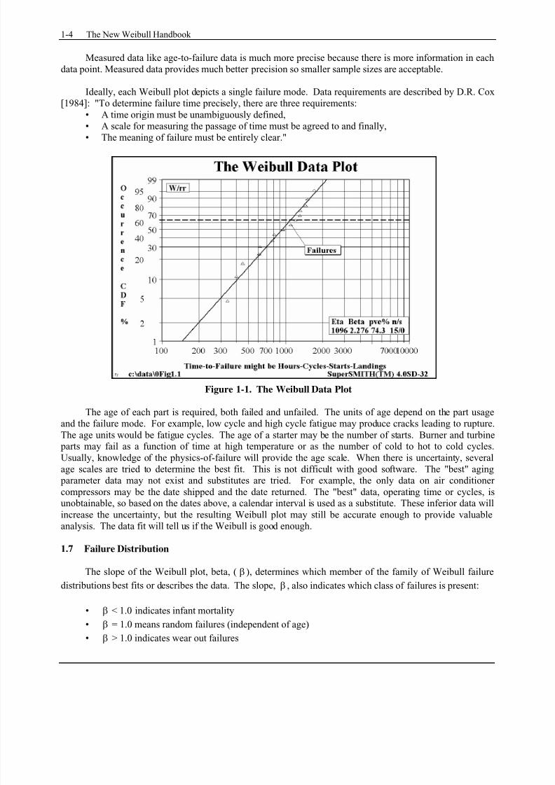
Ideally, each Weibull plot depicts a single failure mode. Data requirements are described by D.R. Cox

[1984]: "To determine failure time precisely, there are three requirements:

• A time origin must be unambiguously defined,

• A scale for measuring the passage of time must be agreed to and finally,

•

The meaning of failure must be entirely clear."

Figure 1-1. The Weibull Data Plot

The age of each part is required, both failed and unfailed. The units of age depend on the part usageand the failure mode. For example, low cycle and high cycle fatigue may produce cracks leading to rupture.

The age units would be fatigue cycles. The age of a starter may be the number of starts. Burner and turbine parts may fail as a function of time at high temperature or as the number of cold to hot to cold cycles.

Usually, knowledge of the physics-of-failure will provide the age scale. When there is uncertainty, several

age scales are tried to determine the best fit. This is not difficult with good software. The "best" aging

parameter data may not exist and substitutes are tried. For example, the only data on air conditioner

compressors may be the date shipped and the date returned. The "best" data, operating time or cycles, isunobtainable, so based on the dates above, a calendar interval is used as a substitute. These inferior data will

increase the uncertainty, but the resulting Weibull plot may still be accurate enough to provide valuable

analysis. The data fit will tell us if the Weibull is good enough.

1.7

Failure Distribution

The slope of the Weibull plot, beta, ( β ), determines which member of the family of Weibull failure

distributions best fits or describes the data. The slope, β , also indicates which class of failures is present:

• β < 1.0 indicates infant mortality

• β = 1.0 means random failures (independent of age)

• β > 1.0 indicates wear out failures



Chapter 1: An Overview of Weibull Analysis 1-5

These classes will be discussed in Chapter 2. The Weibull plot shows the onset of the failure. For example,

it may be of interest to determine the time at which 1% of the population will have failed. Weibull called

this the "B1" life. For more serious or catastrophic failures, a lower risk may be required, B.1 (age at which

0.1% of the population fail) or even B.01 life (0.01% of the population). Six-sigma quality program goals

often equate to 3.4 parts per million (PPM) allowable failure proportion. That would be B.00034! These

values are read from the Weibull plot. For example, on Figure 1-1, the B1 life is approximately 160 and the

B5 life is 300.

The horizontal scale is the age to failure. The vertical scale is the Cumulative Distribution Function

(CDF), describing the percentage that will fail at any age. The complement of the CDF scale,

(100 - CDF) is reliability. The characteristic life η is defined as the age at which 63.2% of the units will

have failed, the B63.2 life, (indicated on the plot with a horizontal dashed line). For β = 1, the mean-time-

to-failure and η are equal. For β > 1.0, MTTF and η are approximately equal. The relationship will be

given in the next chapter.

1.8 Failure Forecasts and Predictions

When failures occur in service, a prediction of the number of failures that will occur in the fleet in the

next period of time is desirable, (say six months, a year, or two years). To accomplish this, the author

developed a risk analysis procedure for forecasting future failures. A typical failure forecast is shown in

Figure 1-2. Cumulative future failures are plotted against future months. This process provides information

on whether the failure mode applies to the entire population or fleet, or to only one portion of the fleet, called

a batch. After alternative plans for corrective action are developed, the failure forecasts are repeated. The

decision-maker will require these failure forecasts to select the best course of action, the plan with the

minimum failure forecast or the minimum cost. If failed parts are replaced as they fail; the failure forecast is

higher than without replacement. Prediction intervals, analogous to confidence intervals, may be added to

the plot. Chapter 4 is devoted to failure forecasting.

Figure 1-2. Failure Forecast




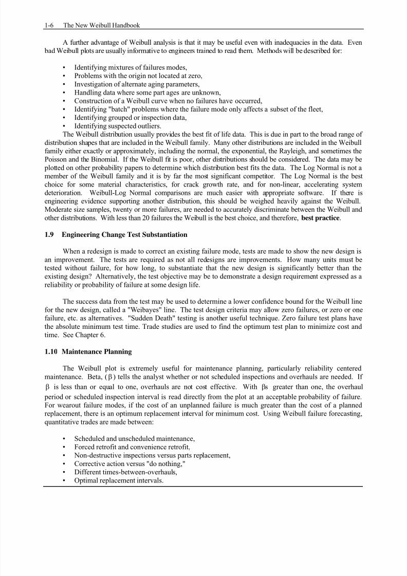
A further advantage of Weibull analysis is that it may be useful even with inadequacies in the data. Even

bad Weibull plots are usually informative to engineers trained to read them. Methods will be described for:

• Identifying mixtures of failures modes,

• Problems with the origin not located at zero,

• Investigation of alternate aging parameters,

• Handling data where some part ages are unknown,

•

Construction of a Weibull curve when no failures have occurred,•

Identifying "batch" problems where the failure mode only affects a subset of the fleet,

• Identifying grouped or inspection data,

• Identifying suspected outliers.

The Weibull distribution usually provides the best fit of life data. This is due in part to the broad range of

distribution shapes that are included in the Weibull family. Many other distributions are included in the Weibull

family either exactly or approximately, including the normal, the exponential, the Rayleigh, and sometimes the

Poisson and the Binomial. If the Weibull fit is poor, other distributions should be considered. The data may be

plotted on other probability papers to determine which distribution best fits the data. The Log Normal is not a

member of the Weibull family and it is by far the most significant competitor. The Log Normal is the best

choice for some material characteristics, for crack growth rate, and for non-linear, accelerating system

deterioration. Weibull-Log Normal comparisons are much easier with appropriate software. If there is

engineering evidence supporting another distribution, this should be weighed heavily against the Weibull.Moderate size samples, twenty or more failures, are needed to accurately discriminate between the Weibull and

other distributions. With less than 20 failures the Weibull is the best choice, and therefore, best practice.

1.9 Engineering Change Test Substantiation

When a redesign is made to correct an existing failure mode, tests are made to show the new design is

an improvement. The tests are required as not all redesigns are improvements. How many units must be

tested without failure, for how long, to substantiate that the new design is significantly better than the

existing design? Alternatively, the test objective may be to demonstrate a design requirement expressed as a

reliability or probability of failure at some design life.

The success data from the test may be used to determine a lower confidence bound for the Weibull linefor the new design, called a "Weibayes" line. The test design criteria may allow zero failures, or zero or one

failure, etc. as alternatives. "Sudden Death" testing is another useful technique. Zero failure test plans have

the absolute minimum test time. Trade studies are used to find the optimum test plan to minimize cost and

time. See Chapter 6.

1.10 Maintenance Planning

The Weibull plot is extremely useful for maintenance planning, particularly reliability centered

maintenance. Beta, (β ) tells the analyst whether or not scheduled inspections and overhauls are needed. If

β is less than or equal to one, overhauls are not cost effective. With sβ greater than one, the overhaul

period or scheduled inspection interval is read directly from the plot at an acceptable probability of failure.

For wearout failure modes, if the cost of an unplanned failure is much greater than the cost of a plannedreplacement, there is an optimum replacement interval for minimum cost. Using Weibull failure forecasting,

quantitative trades are made between:

•

Scheduled and unscheduled maintenance,

• Forced retrofit and convenience retrofit,

•

Non-destructive inspections versus parts replacement,

• Corrective action versus "do nothing,"

• Different times-between-overhauls,

•

Optimal replacement intervals.




Planned maintenance induces cyclic or rhythmic changes in failure rates. The rhythm is affected by

the interactions between characteristic lives of the failure modes of the system, sβ , the inspection periods,

and parts replacements. This phenomenon is illustrated in Chapter 4.

1.11 System Analysis and Math Models

Mathematical models of components and entire systems like a sports car, a big truck, or a nuclear

power system may be produced by combining (statisticians say convoluting) tens or hundreds of failuremodes. Most of these modes are represented by Weibulls but some may be Lognormal, or even Binomial.

The combination may be done by Monte Carlo simulation or by analytical methods. If the data cannot be

segregated into individual failure modes or if the early data is missing, the Crow-AMSAA or the Kaplan-

Meier models may still be applied to provide trending and failure forecasting. System models are useful for

predicting spare parts usage, availability, module returns to depot, and maintainability support costs. These

models are frequently updated with the latest Weibulls. Predictions may be compared with actual results to

estimate the model uncertainties and fine-tune the model.

If the data from a system, such as a diesel engine, are not adequate to plot individual failure modes, it

is tempting to plot a single Weibull for the system. This plot will show a β close to one. This is roughly

equivalent to using mean-time-to-failure (MTTF) and exponential reliability. It masks infant mortality and

wear out modes. This approach is not recommended, as the results are not meaningful for the individual

failure modes. This method was common in the fifties and sixties and is still used by those unaware of theadvantages of Weibull Analysis and the newer methods for system models. Better methods are provided for

these data deficiencies. See Chapter 8.

Figure 1-3 Bearings Rarely Fail Early in Life Weibulls With Curved Data




1.12 Weibulls with Curved Data

The Weibull plot is inspected to determine how well the failure data fit a straight line. Sometimes the

failure points do not fall along a straight line on the Weibull plot, and modification of the simple Weibull

approach is required. The data are trying to tell us something in these cases. Weibull illustrated this concept

in his 1951 paper. The bad fit may relate to the physics of the failure or to the quality of the data. If the

points fall on gentle curves, it may be that the origin of the age scale is not located at zero. See Figure 1-3.

There are usually physical reasons for this. The manufacturer may not have reported early failures thatoccurred in production acceptance. With roller bearing unbalance, it takes many rotations for the wobbling

roller to destroy the cage. The bearing cannot fail instantaneously. This leads to an origin correction equal

to the minimum time necessary to fail. The correction is called 0t , and if it is positive, it provides a

guaranteed failure free period from zero to time 0t . If the correction is negative, "old" parts, perhaps with

shelf life aging, may be the cause. The 0t correction is treated in Chapter 3.

Lognormal data plotted on Weibull probability paper will appear curved, concave downward like

Figure 1-3. Therefore, the Weibull with the 0t correction and the Lognormal distribution are candidates for

distributional analysis to tell us which is the best distribution. The critical correlation coefficient provides an

easy solution. This capability is in WinSMITH Weibull (WSW). Moderate size samples are required to

discriminate between these distributions, at least 20 failures. Otherwise the standard two parameter Weibullis the best choice [Lui].

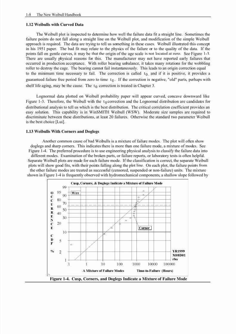
1.13 Weibulls With Corners and Doglegs

Another common cause of bad Weibulls is a mixture of failure modes. The plot will often show

doglegs and sharp corners. This indicates there is more than one failure mode, a mixture of modes. See

Figure 1-4. The preferred procedure is to use engineering physical analysis to classify the failure data into

different modes. Examination of the broken parts, or failure reports, or laboratory tests is often helpful.

Separate Weibull plots are made for each failure mode. If the classification is correct, the separate Weibull

plots will show good fits, with their points falling along the plot line. On each plot, the failure points from

the other failure modes are treated as successful (censored, suspended or non-failure) units. The mixture

shown in Figure 1-4 is frequently observed with hydromechanical components, a shallow slope followed by

Figure 1-4. Cusp, Corners, and Doglegs Indicate a Mixture of Failure Mode




a steep slope. For this classic mixture, if additional failure analysis is impossible, a statistical solution based

on the likelihood ratio test may provide the separate Weibull failure modes. Appendixes F and J provide a

discussion of more complex mixtures including batch problems.

As the number of failure modes mixed together increases to say five or more, the doglegs and corners

tend to disappear and β will tend toward one (unless all the modes have the same β and similar η ). See

Section 3.7.

1.14 Weibayes

A Weibull plot may be needed even when no failures have occurred. For example, an engineering redesign

is made to correct a failure mode experienced in service. Redesigned units are tested to prove that the problem is

corrected. How many units must be tested for how long to have statistical confidence that the problem is solved?

When parts exceed their design life, it may be possible to extend their life by constructing a Weibull with no

failures. The method is called Weibayes analysis. It has many applications and is presented in Chapter 6.

Methods to design experiments to substantiate new designs using Weibayes theory is also presented in Chapter 6.

In preliminary design, when there is little or no data on the new designs, Weibayes may be used to estimate the

Weibulls for the new design. If the number of failures is extremely small and there is good prior knowledge of the

slope, β , Weibayes will be more accurate than the Weibull.

1.15 Small Sample Weibulls

Statisticians always prefer large samples of data, but engineers are forced to do Weibull or Weibayes

analysis with very small samples, even as few as one to three failures. When the result of a failure involves

safety or extreme costs, it is inappropriate to request more failures. The primary advantage of Weibull

analysis is that engineering objectives can often be met even with extremely small samples. Of course, smallsamples always imply large uncertainties. To evaluate these small sample uncertainties, confidence bounds

are available in WSW. Chapter 7 is devoted to confidence methods.

1.16 Updating Weibulls

After the initial Weibull, later plots may be based on larger failure samples and more time on

successful units. Each updated plot will be slightly different, but gradually the Weibull parameters, β and

η , will stabilize and approach the true Weibull as the data sample increases. With the appropriate fit

method, the important engineering inferences about B.1 life and the failure forecasts will not change

significantly as the sample size increases. With complete samples (no suspensions) β and η oscillate

around the true unknown value.

1.17 Deficient (Dirty) Data

Special methods have been developed for many forms of "dirty" data including:

• Censored-suspended data • No failure data

•

Mixtures of failure modes • Nonzero time origin

•

Failed units not identified • Extremely small samples

• Inspection data & coarse data • Early data missing

•

Suspension times or ages missing • Data plots with curves and doglegs




1.18 Establishing the Weibull Line, Choosing the Fit Method

The standard engineering method for establishing the Weibull line is to plot the time to failure data on

Weibull probability graphs using median rank plotting positions described in Chapter 2. Statisticians,

however, prefer an analytical method called maximum likelihood. The likelihood calculations require a

computer. Both methods have advantages and disadvantages. The pros and cons will be discussed in

Chapter 5. There are also special methods for different types of inspection data and warranty data that are

treated in Chapters 5 and 8. The author recommends the best practice among these alternatives dependingon the data. The reasons and research for these recommendations are provided.

1.18

Related Methods and Problems

Weibull analysis is the main theme of this text, but there are some types of data and some types of

problems that can be analyzed better with other math models that are described later. For example, the

Weibull distribution is also the Extreme Value Type III minimum distribution. The Extreme Value Type I

is called the Gumbel distribution and both the minimum and maximum forms may have useful applications.

For example gust loads on aircraft are modeled with Gumbel maximum distribution. See Figure 1-5.

Some organizations feel the Crow-AMSAA (C-A) model is more important than Weibull analysis. Itis extremely useful. It is more robust that Weibull, that is, it provides reasonable accurate results when the

data has serious deficiencies. It works well even with mixtures of failure modes and missing portions of

data. Weibull plots allow only one failure mode at a time. It will track changes in reliability which Weibull

cannot. C-A is the best tool for trending significant events for management, such as outages, production

cutbacks and interruptions, accidents, and in-flight loss of power. The original C-A objective was to track

the growth of reliability in R&D testing. It is still best practice for that application. It is also best practice

for predicting warranty claims by calendar time and tracking systems in-service.

Figure 1-5. NACA Wind Gust Loads Gumbel + Distribution

Kaplan-Meier (K-M) survival analysis is a good for "snapshot" data, (a large portion of initial data is

not available). This tool was developed in the medical industry and has good statistical properties. We have




borrowed K-M for our reliability work. K-M is also used for warranty claim predictions as a function of age,

and for some forms of inspection data.

Wayne Nelson's Graphical Repair Analysis provides a rigorous approach for predicting warranty

claims by age of the units when repeated warranty repairs of the same type are expected.

1.20 Summary

Chapter 1 has provided an overview of Weibull analysis. There are many methods because there are

many kinds of data and applications. The real effort involved with this Weibull analysis is obtaining and

validating good data. The analysis, given good software, is almost trivial by comparison.

• The next chapter (2) will discuss good Weibull plots and good data and the standard method of

analysis.

• Chapter 3 will treat bad Weibulls and "dirty" data. Case studies will be employed to illustrate the

methods and solutions.

•

Chapter 4 is devoted to failure forecasting, Monte Carlo, and optimal parts replacement intervals.

•

Chapter 5 presents alternative data formats and special solution methods.

•

The Weibayes concept, substantiation tests and Weibull Libraries are treated in Chapter 6.

• Chapter 7 discusses confidence intervals and testing two or more data sets to see if they are

significantly different.

•

Chapter 8 treats a number of related math models.

•

Chapter 9 presents Crow-AMSAA modeling and warranty analysis.

•

Chapter 10 summarizes the methods, analysis, and interpretations of the plots. Bob Rock's logic

diagram in Chapter 10 will lead you step-by-step though the best practices for your particular data.

• Chapter 11 is a collection of interesting case studies contributed by industry experts

There is little herein on qualitative methods, as the emphasize is on quantitative methods. However,

qualitative methods are extremely important. Failure reporting and analysis (FRACAS) is required for

accurate life data analysis. Failure mode and effect analysis (FEMA) and fault tree analysis can

significantly improve the design process and are needed to identify the root cause of failure modes. Design

review is prerequisite to achieving high reliability and is significantly improved by use of a Weibull library

to avoid previous design mistakes. Pat [O’Connor] provides a good introduction to these methods. The

Weibull library is discussed in Chapter 6.

A comment on software is appropriate here. As the primary purpose of this Handbook is to be the

workbook for the Weibull Workshops, it is necessary to present the software capabilities with the

methodology. Further, for readers not attending the workshop, good software is needed to eliminate the

drudgery of hand calculations and in general, increases the productivity of the analyst many times over. The

author has been deeply involved in the development of

WinSMITH Weibull (WSW) & WinSMITH Visual (WSV)

software and therefore, recommends their features and

friendly characteristics. Further, no other software does all

the methods presented in the Handbook. Almost all of the

plots herein are from SuperSMITH, a bundled set of

Windows software including WinSMITH Weibull and

Visual as well as YBATH. This software is used in our

Weibull Workshops. Free "demo" versions of the software

are available on our web site. Wes Fulton is the creator of

the software and with the author, is available to answer

questions concerning applications. Our addresses and

phone numbers are given on the back cover and the

backside of the title pages. We would like to hear from you.

inse6320_lecture notes week 4

Documents