Inference for the mean vector

- one-sample and two-samples,

overview

1

Univariate Inference

Let x1, x2, … , xn denote a sample of n from the normal distribution with mean m and variance s2.

Suppose we want to test

H0: m = m0 vs

HA: m ≠ m0

The appropriate test is the t test:

The test statistic:

Reject H0 if |t| > ta/2

0xt n

s

m

2

The multivariate Test

Let denote a sample of n from the p-variate

normal distribution with mean vector and covariance

matrix S.

Suppose we want to test

1 2, , , nx x xm

0 0

0

: vs

:A

H

H

m m

m m

3

Roy’s Union- Intersection Principle

This is a general procedure for developing a

multivariate test from the corresponding univariate test.

1

i.e. observation vector

p

X

X

X

1. Convert the multivariate problem to a univariate problem by

considering an arbitrary linear combination of the

observation vector.

1 1 p pU a X a X a X

arbitrary linear combination of the observations

4

2. Perform the test for the arbitrary linear combination of the

observation vector.

3. Repeat this for all possible choices of

1

p

a

a

a

4. Reject the multivariate hypothesis if H0 is rejected for any

one of the choices for

5. Accept the multivariate hypothesis if H0 is accepted for all

of the choices for

6. Set the type I error rate for the individual tests so that the

type I error rate for the multivariate test is a.

.a

.a

5

Let denote a sample of n from the p-variate

normal distribution with mean vector and covariance

matrix S.

Suppose we want to test

1 2, , , nx x xm

0 0

0

: vs

:A

H

H

m m

m m

Application of Roy’s principle to the following situation

1 1Let i i i p piu a x a x a x

Then u1, …. un is a sample of n from the normal

distribution with mean and variance . a m a aΣ6

to test

0 0

0

: vs

:

a

a

A

H a a

H a a

m m

m m

we would use the test statistic:

0a

u

u at n

s

m

1 1

1 1Now

n n

i i

i i

u u a xn n

1 1

1 1n n

i i

i i

a x a x a xn n

7

and

222

1 1

1 1

1 1

n n

u i i

i i

s u u a x a xn n

2

1

1

1

n

i

i

a x xn

1

1

1

n

i i

i

a x x x x an

8

= 𝑎 ′1

𝑛 − 1 𝑥 𝑖 − 𝑥 𝑥 𝑖 − 𝑥

′𝑛

𝑖=1𝑎 = 𝑎 ′𝑆𝑎

Thus

00

a a x a nt n a x

a aa a

mm

SS

We will reject 0 0:aH a am m

if 0 / 2

a nt a x t

a a am

S

2

2 0 2

/ 2or a

n a xt t

a a a

m

S

9

We will reject

0 0 0: in favour of :AH Hm m m m

Using Roy’s Union- Intersection principle:

2

2 0 2

/ 2if for at least one a

n a xt t a

a a a

m

S

We accept 0 0:H m m

2

2 0 2

/ 2if for all a

n a xt t a

a a a

m

S

10

We reject

0 0:H m m

i.e.

2

0 2

/ 2if max

a

n a xt

a a a

m

S

We accept 0 0:H m m

2

0 2

/ 2if max

a

n a xt

a a a

m

S

11

Consider the problem of finding:

2

0

max maxa a

n a xh a

a a

m

Swhere

2

0 0 0n a x a x x a

h a na a a a

m m m S S

0 0 0 0

2

2 2

0

a a x x a a x x a ah a

na a a

m m m m

S S

S

0 0or a a x a x am m

S S

12

thus

2

0

maxopt

aopt opt

n a xh a

a a

m

S

1 1

0 0

0

or opt

a aa x k x a

a xm m

m

SS S

2

1

0 0

2 1 1

0 0

n k x x

k x x

m m

m m

S

S SS

1

0 0n x xm m S

13

We reject 0 0:H m m

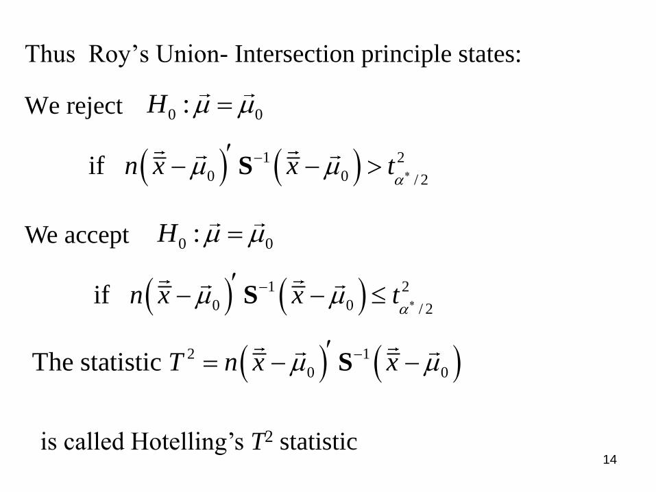
Thus Roy’s Union- Intersection principle states:

1 2

0 0 / 2if n x x t

am m

S

We accept 0 0:H m m

1 2

0 0 / 2if n x x t

am m

S

2 1

0 0The statistic T n x xm m S

is called Hotelling’s T2 statistic 14

We reject 0 0:H m m

Choosing the critical value for Hotelling’s T2 statistic

2 1 2

0 0 / 2if T n x x t

am m

S

2

/ 2To determine t

a , we need to find the sampling

distribution of T2 when H0 is true.

It turns out that if H0 is true than

2 1

0 0 1 1

n p nn pF T x x

p n p nm m

S

has an F distribution with n1 = p and n2 = n - p 15

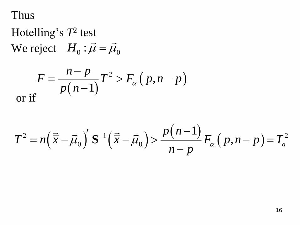
We reject 0 0:H m m

Thus

Hotelling’s T2 test

2 1 2

0 0

1, a

p nT n x x F p n p T

n pam m

S

2 ,

1

n pF T F p n p

p na

or if

16

f x

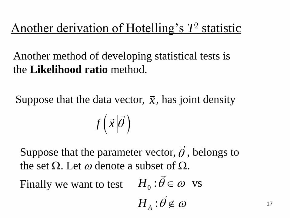
Another derivation of Hotelling’s T2 statistic

Another method of developing statistical tests is

the Likelihood ratio method.

Suppose that the data vector, , has joint density x

Suppose that the parameter vector, , belongs to

the set W. Let w denote a subset of W.

Finally we want to test 0 : vs

:A

H

H

w

w

17

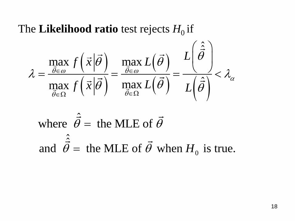
ˆ̂

max max

ˆmaxmax

Lf x L

Lf x L

w wa

WW

The Likelihood ratio test rejects H0 if

ˆwhere the MLE of

0

ˆ̂and the MLE of when is true.H

18

The situation

Let denote a sample of n from the p-variate

normal distribution with mean vector and covariance

matrix S.

Suppose we want to test

1 2, , , nx x xm

0 0

0

: vs

:A

H

H

m m

m m

19

The Likelihood function is:

1

1

1

2

/ 2 / 2

1, e

2

n

i i

i

x x

np nL

m m

m

S S

S

and the Log-likelihood function is:

, ln , l Lm mS S

1

1

1ln 2 ln

2 2 2

n

i i

i

np nx x m m

S S

20

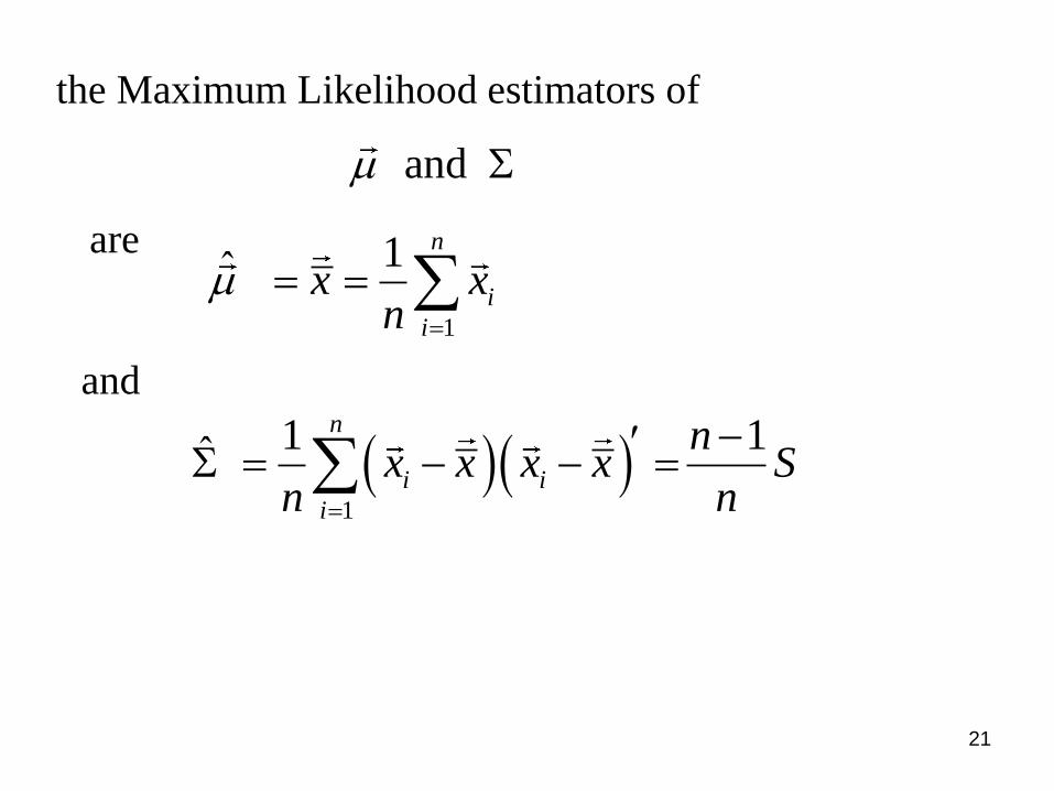
and m S

the Maximum Likelihood estimators of

are

1

1ˆ n

i

i

x xn

m

and

1

1 1ˆ n

i i

i

nx x x x S

n n

S

21

and m Sthe Maximum Likelihood estimators of

when H 0 is true are:

0

ˆ̂ˆ m m

and

0 0

1

1ˆ̂

n

i i

i

x xn

m m

S

22

The Likelihood function is:

1

1

1

2

/ 2 / 2

1, e

2

n

i i

i

x x

np nL

m m

m

S S

S

now

1

1

1

n

ni in

i

tr x x S x x

1

1

1

n

ni in

i

tr S x x x x

23

1

1

1

n

ni in

i

tr S x x x x

1 11 = 1 = n n

n ntr n I n p np

Thus

2/ 2/ 2

1

1ˆ ˆ, 2

np

nnpnn

L eS

m

S

similarly

2/ 2

/ 2

1ˆ ˆˆ ˆ, ˆ̂

2

np

nnp

L em

S

S

24

and

/ 2 / 21 1

/ 2 / 2

0 0

1

ˆ ˆˆ ˆ,

ˆ ˆ ˆ, 1ˆ

n nn nn n

n nn

i i

i

LS S

Lx x

n

m

m

m m

S

S S

/ 2

/ 2

0 0

1

1

n

nn

i i

i

n S

x xm m

25

Note:

11 12

21 22

A A u wA

A A w V

Let

1

11 22 21 11 12

1

22 11 12 22 21

A A A A AA

A A A A A

1

1u V ww

u

V u w V w

11Thus u V ww V u w V w

u

26

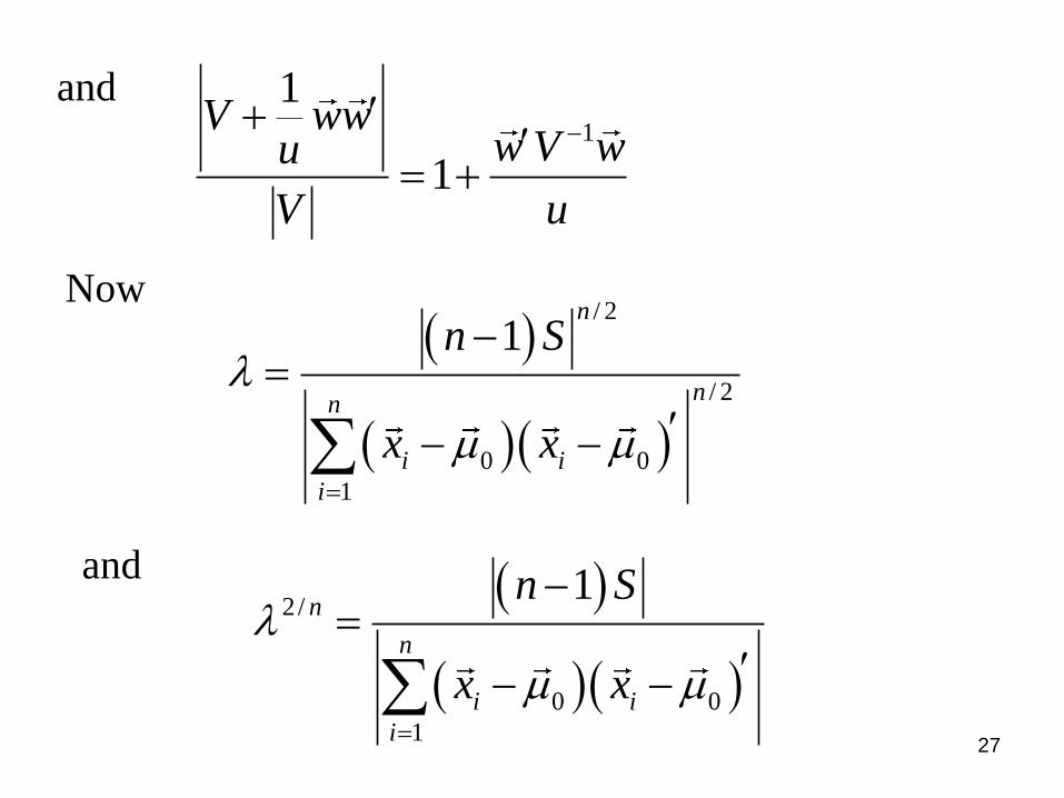
and

1

1

1

V www V wu

V u

/ 2

/ 2

0 0

1

1

n

nn

i i

i

n S

x x

m m

Now

and

2/

0 0

1

1 n

n

i i

i

n S

x x

m m

27

Also

0 0 0 0

1 1

= n n

i i i i

i i

x x x x x x x xm m m m

0

1 1

=n n

i i i

i i

x x x x x x xm

0 0 0

1

n

i

i

x x x n x xm m m

0 0

1

=n

i i

i

x x x x n x xm m

0 0

1

=n

i i

i

x x x x n x xm m

0 0= 1n S n x xm m

28

Thus

2/

0 0

1

1 n

n

i i

i

n S

x x

m m

0 0

1

1

n S

n S n x xm m

0 0

1

S

nS x x

nm m

29

Thus

0 02/ 1

n

nS x x

n

S

m m

using 1

1

1

V www V wu

V u

0

1,

and

u n

V S

w n x m

30

Then 1

0 02/ 1 1

nn x S x

n

m m

Thus to reject H0 if < a 2/i.e. n n

a

2/or n n

a

1

0 0and 1

1

nn x S x

na

m m

1

0 0or 1 -1 nn x S x n am m

This is the same as Hotelling’s T2 test if

2/1

1 -1 , np n

n T F p n pn p

a a a

31

Example

For n = 10 students we measure scores on

– Math proficiency test (x1),

– Science proficiency test (x2),

– English proficiency test (x3) and

– French proficiency test (x4)

The average score for each of the tests in previous

years was 60. Has this changed?

32

The data

Student Math Science Eng French

1 81 89 73 74

2 73 79 73 74

3 61 86 81 81

4 55 70 76 73

5 61 71 61 66

6 52 70 56 58

7 56 74 56 56

8 65 87 73 69

9 54 76 69 72

10 48 71 62 63

33

Summary Statistics

60.6

77.3

68.0

68.6

x

S

102.044 56.689 41.222 39.489

56.689 56.456 42.000 35.356

41.222 42.000 75.778 65.111

39.489 35.356 65.111 61.378

0.0245 -0.0255 0.0195 -0.0218

-0.0255 0.0567 -0.0405 0.0267

0.0195 -0.0405 0.1782 -0.1783

-0.0218 0.0267 -0.1783 0.2040

1

: S

Note

2 1

0 0 151.135T n x S xm m

0.05 0.05 0.05

1 4 9 4 9, 4,6 = 4.53 27.18

6 6

p nT F p n p F

n p

0

m

60

60

60

60

34

Simultaneous Inference for means

Recall

2 1T n x S xm m

2

2

1max max

a a

n a x at a

a S a

m

(Using Roy’s Union Intersection Principle)

35

Now

2 1P T T P n x S x Ta am m

2

1max

a

n a x aP T

a S aa

m

2

1 for all

n a x aP T a

a S aa

m

1

2

for all a S a

P a x a T an

am

1 a 36

Thus

1 1

for all a S a a S a

P a x T a a x T an n

a am

1 a

and the set of intervals

1 1

to a S a a S a

a x T a x Tn n

a a

Form a set of (1 – a)100 % simultaneous

confidence intervals for a m37

Recall

,-1

= p n pn p

T Fn p

a a

1,

-1 p n p

n pa S aa x F

n n pa

Thus the set of (1 – a)100 % simultaneous

confidence intervals for a m

1,

-1to p n p

n pa S aa x F

n n pa

38

The two sample problem

39

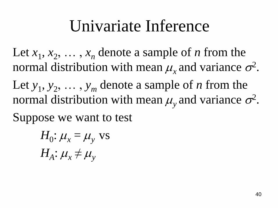
Univariate Inference

Let x1, x2, … , xn denote a sample of n from the

normal distribution with mean mx and variance s2.

Let y1, y2, … , ym denote a sample of n from the

normal distribution with mean my and variance s2.

Suppose we want to test

H0: mx = my vs

HA: mx ≠ my

40

The appropriate test is the t test:

The test statistic:

Reject H0 if |t| > ta/2 d.f. = n + m -2

1 1pooled

x yt

sn m

2 21 1

2

x y

pooled

n s m ss

n m

41

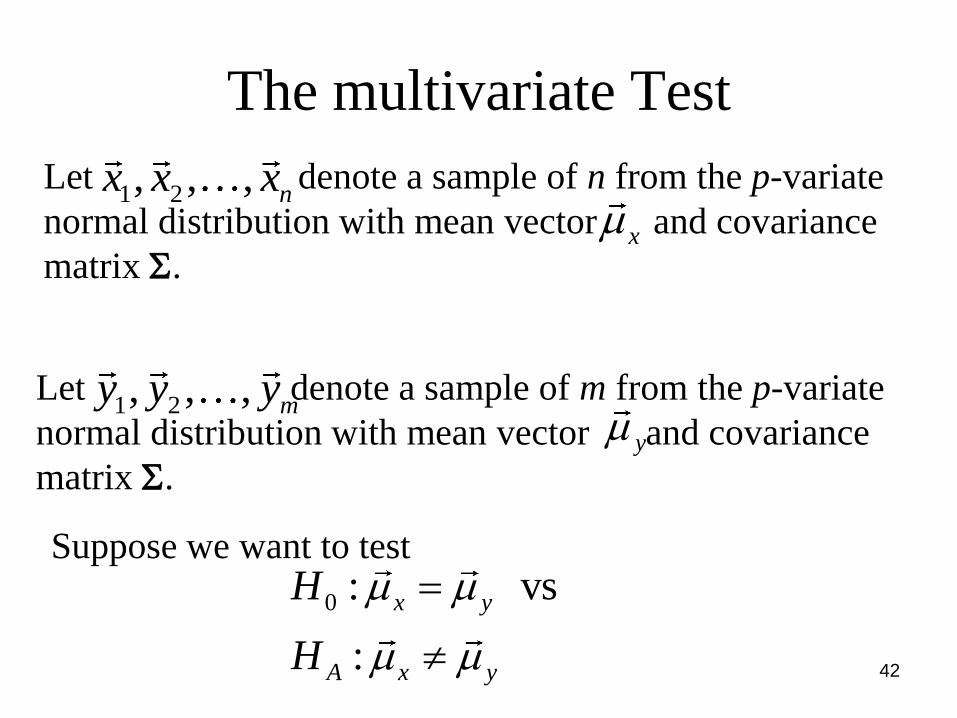
The multivariate Test

Let denote a sample of n from the p-variate

normal distribution with mean vector and covariance

matrix S.

1 2, , , nx x x

xm

0 : vs

:

x y

A x y

H

H

m m

m m

Suppose we want to test

Let denote a sample of m from the p-variate

normal distribution with mean vector and covariance

matrix S.

1 2, , , my y yym

42

Hotelling’s T2 statistic for the two sample problem

2 11

1 1pooledT x y x y

n m

S

if H0 is true than

21

2

n m pF T

p n m

has an F distribution with n1 = p and

n2 = n +m – p - 1

1 1

2 2pooled x y

n m

n m n m

S S S

43

We reject 0 : x yH m m

Thus

Hotelling’s T2 test

21

if , 12

n m pF T F p n m p

p n ma

2 11with

1 1pooledT x y x y

n m

S

1 1

2 2pooled x y

n m

n m n m

S S S

44

Simultaneous inference for the

two-sample problem

• Hotelling’s T2 statistic can be shown to have

been derived by Roy’s Union-Intersection

principle

2 11namely

1 1pooledT x y x y

n m

S

2

2max max1 1a a

pooled

a x yt a

a an m

S

where x y m m 45

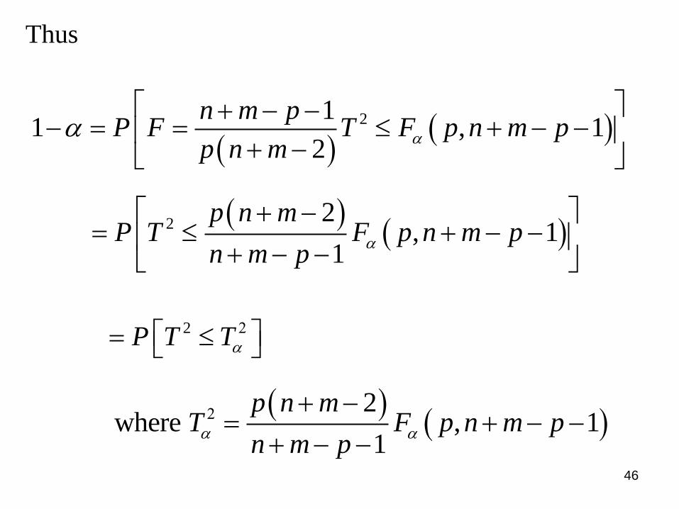
Thus

21

1 , 12

n m pP F T F p n m p

p n maa

2

2, 1

1

p n mP T F p n m p

n m pa

2P T Ta

2where , 1

1

p n mT F p n m p

n m pa a

46

Thus

2

max 11 1a

pooled

a x yP T

a an m

a

a

S

2

or for all 11 1

pooled

a x yP T a

a an m

a

a

S

47

Thus

2 1 1

for all 1pooledP a x y T a a an m

a a S

Hence

1 1

pooled x yP a x y T a a an m

a m m

S

1 1

for all 1pooleda x y T a a an m

a a

S

48

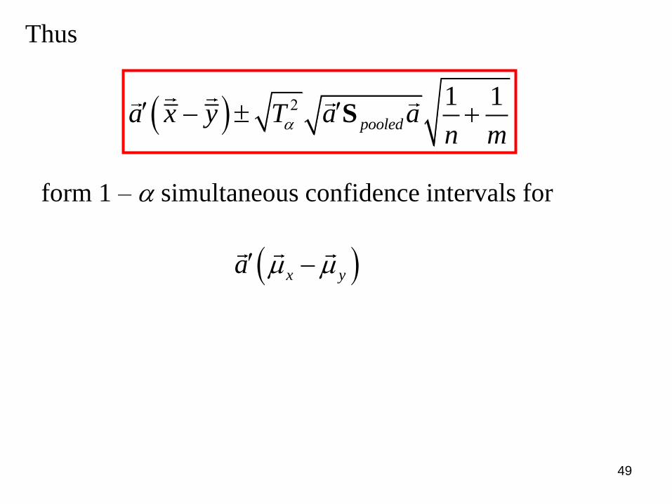
Thus

form 1 – a simultaneous confidence intervals for

1 1

pooleda x y T a an m

a

S

x ya m m

49

Example Annual financial data are collected for firms approximately 2 years prior to bankruptcy and for financially sound firms at about the same point in time. The data on the four variables

• x1 = CF/TD = (cash flow)/(total debt),

• x2 = NI/TA = (net income)/(Total assets),

• x3 = CA/CL = (current assets)/(current liabilties, and

• x4 = CA/NS = (current assets)/(net sales) are given in the following table.

50

The data are given in the following table:

Bankrupt Firms Nonbankrupt Firms

x1 x2 x3 x4 x1 x2 x3 x4

Firm CF/TD NI/TA CA/CL CA/NS Firm CF/TD NI/TA CA/CL CA/NS

1 -0.4485 -0.4106 1.0865 0.4526 1 0.5135 0.1001 2.4871 0.5368 2 -0.5633 -0.3114 1.5314 0.1642 2 0.0769 0.0195 2.0069 0.5304 3 0.0643 0.0156 1.0077 0.3978 3 0.3776 0.1075 3.2651 0.3548 4 -0.0721 -0.0930 1.4544 0.2589 4 0.1933 0.0473 2.2506 0.3309

5 -0.1002 -0.0917 1.5644 0.6683 5 0.3248 0.0718 4.2401 0.6279 6 -0.1421 -0.0651 0.7066 0.2794 6 0.3132 0.0511 4.4500 0.6852 7 0.0351 0.0147 1.5046 0.7080 7 0.1184 0.0499 2.5210 0.6925 8 -0.6530 -0.0566 1.3737 0.4032 8 -0.0173 0.0233 2.0538 0.3484 9 0.0724 -0.0076 1.3723 0.3361 9 0.2169 0.0779 2.3489 0.3970 10 -0.1353 -0.1433 1.4196 0.4347 10 0.1703 0.0695 1.7973 0.5174 11 -0.2298 -0.2961 0.3310 0.1824 11 0.1460 0.0518 2.1692 0.5500 12 0.0713 0.0205 1.3124 0.2497 12 -0.0985 -0.0123 2.5029 0.5778 13 0.0109 0.0011 2.1495 0.6969 13 0.1398 -0.0312 0.4611 0.2643 14 -0.2777 -0.2316 1.1918 0.6601 14 0.1379 0.0728 2.6123 0.5151 15 0.1454 0.0500 1.8762 0.2723 15 0.1486 0.0564 2.2347 0.5563 16 0.3703 0.1098 1.9914 0.3828 16 0.1633 0.0486 2.3080 0.1978

17 -0.0757 -0.0821 1.5077 0.4215 17 0.2907 0.0597 1.8381 0.3786 18 0.0451 0.0263 1.6756 0.9494 18 0.5383 0.1064 2.3293 0.4835 19 0.0115 -0.0032 1.2602 0.6038 19 -0.3330 -0.0854 3.0124 0.4730 20 0.1227 0.1055 1.1434 0.1655 20 0.4875 0.0910 1.2444 0.1847 21 -0.2843 -0.2703 1.2722 0.5128 21 0.5603 0.1112 4.2918 0.4443 22 0.2029 0.0792 1.9936 0.3018 23 0.4746 0.1380 2.9166 0.4487 24 0.1661 0.0351 2.4527 0.1370 25 0.5808 0.0371 5.0594 0.1268

51

Hotelling’s T2 test

A graphical explanation

52

Hotelling’s T2 statistic for the two sample problem

2 11

1 1pooledT x y x y

n m

S

1 1where

2 2pooled x y

n m

n m n m

S S S

53

2

2 2max max1 1a a

pooled

a x yT t a

a an m

S

: 1 1

pooled

a x a yt a

a an m

Note

S

is the test statistic for testing:

0 : vs :x y A x yH a a a H a a am m m m

54

Popn A

Popn B

X1

X2

Hotelling’s T2 test

55

Popn A

Popn B

X1

X2

Univariate test for X1

56

Popn A

Popn B

X1

X2 Univariate test for X2

57

Popn A

Popn B

X1

X2 Univariate test for a1X1 + a2X2

58

Mahalanobis distance

A graphical explanation

59

22

1

,p

i i

i

d a b a b a b a b

Euclidean distance

a

points equidistant

from a

60

2 ,Md a b a b a bS S

Mahalanobis distance: S, a covariance matrix

a

points equidistant

from a

61

Hotelling’s T2 statistic for the two sample problem

2 1 21 1, ,pooled M pooledT x y x y d x y

n m

S S

2 11

1 1pooledT x y x y

n m

S

1

pooled

nmx y x y

n m

S

2 , ,M pooled

n md x y

nm

S

62

Popn A

Popn B

X1

X2

Case I

63

Popn A

Popn B

X1

X2

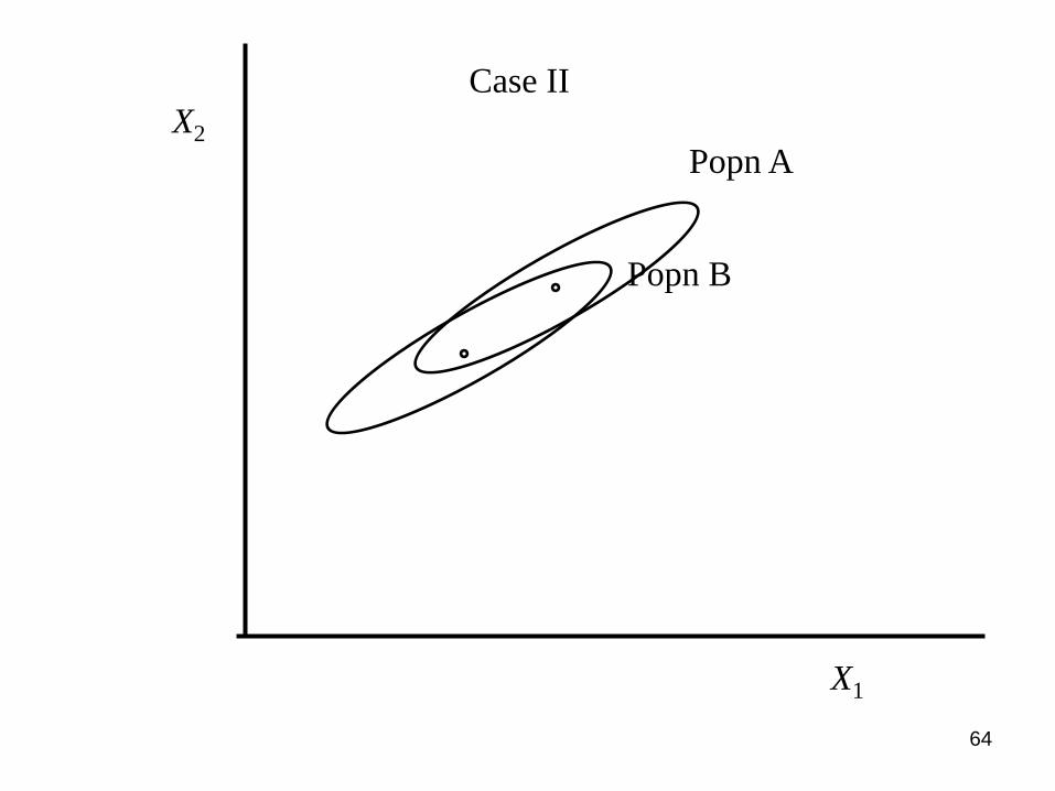
Case II

64

Popn A

Popn B

X1

X2

Case I

Popn A

Popn B

X1

X2

Case II

In Case I the Mahalanobis distance between the mean

vectors is larger than in Case II, even though the

Euclidean distance is smaller. In Case I there is more

separation between the two bivariate normal

distributions

65

Related websites

• SAS & R-code:

• http://www.public.iastate.edu/~maitra/stat501/RSAS.html

• https://onlinecourses.science.psu.edu/stat505/node/124

• Wikipedia:

• https://en.wikipedia.org/wiki/Hotelling%27s_T-

squared_distribution

• https://en.wikipedia.org/wiki/Harold_Hotelling

• Multivariate Observations, by G. A. F. Seber

http://onlinelibrary.wiley.com/book/10.1002/9780470316641

• Applied Multivariate Statistics with SAS® Software, 2nd

Edition, By Ravindra Khattree and Dayanand N. Naik

66